Tracking of Vector Field Singularities in Unstructured 3D Time-Dependent

Datasets

Christoph Garth

University of Kaiserslautern

Xavier Tricoche

University of Utah

Gerik Scheuermann

University of Kaiserslautern

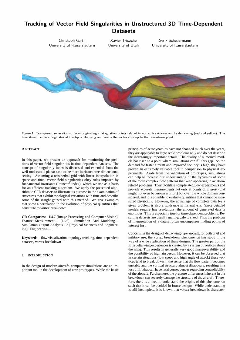
Figure 1: Transparent separation surfaces originating at stagnation points related to vortex breakdown on the delta wing (red and yellow). Theblue stream surface originates at the tip of the wing and wraps the vortex core up to the breakdown point.

ABSTRACT

In this paper, we present an approach for monitoring the posi-tions of vector field singularities in time-dependent datasets. Theconcept of singularity index is discussed and extended from thewell-understood planar case to the more intricate three-dimensionalsetting. Assuming a tetrahedral grid with linear interpolation inspace and time, vector field singularities obey rules imposed byfundamental invariants (Poincare index), which we use as a basisfor an efficient tracking algorithm. We apply the presented algo-rithm to CFD datasets to illustrate its purpose in the examination ofstructures that exhibit topological variations with time and describesome of the insight gained with this method. We give examplesthat show a correlation in the evolution of physical quantities thatconstitute to vortex breakdown.

CR Categories: I.4.7 [Image Processing and Computer Vision]:Feature Measurement— [I.6.6]: Simulation And Modeling—Simulation Output Analysis J.2 [Physical Sciences and Engineer-ing]: Engineering—.

Keywords: flow visualization, topology tracking, time-dependentdatasets, vortex breakdown

1 INTRODUCTION

In the design of modern aircraft, computer simulations are an im-portant tool in the development of new prototypes. While the basic

principles of aerodynamics have not changed much over the years,they are applicable to large scale problems only and do not describethe increasingly important details. The quality of numerical mod-els has risen to a point where simulations can fill this gap. As thedemand for faster aircraft and improved security is high, they haveproven an extremely valuable tool in comparison to physical ex-periments. Aside from the validation of prototypes, simulationscan help to increase our understanding of the dynamics of someof the more complex flow patterns that keep appearing in aviation-related problems. They facilitate complicated flow experiments andprovide accurate measurements not only at points of interest (thatmight not even be known a priori) but over the whole domain con-sidered, and it is possible to evaluate quantities that cannot be mea-sured physically. However, the advantage of complete data for agiven problem is also a hindrance in its analysis. Since detailedmodels require fine resolutions, the amount of generated data isenormous. This is especially true for time-dependent problems. Re-sulting datasets are usually multi-gigabyte sized. Thus the problemof interpretation of a dataset often encompasses finding points ofinterest first.

Concerning the design of delta-wing type aircraft, for both civil andmilitary use, the vortex breakdown phenomenon has stood in theway of a wide application of these designs. The greater part of thelift a delta wing experiences is created by a system of vortices abovethe wing. This results in generally very good maneuverability andthe possibility of high airspeeds. However, it can be observed thatin certain situations (low speed and high angle of attack) these vor-tices tend to break down in the sense that the flow pattern becomesunstable and the vortical structure almost disappears, resulting in aloss of lift that can have fatal consequences regarding controllabilityof the aircraft. Furthermore, the pressure differences inherent in thebreakdown can severely damage the structure of the aircraft. There-fore, there is a need to understand the origins of this phenomenonsuch that it can be avoided in future designs. While understandingis still incomplete, it is known that vortex breakdown is character-

ized by the appearance of stagnation points on the axis of the pri-mary vortices[8]. Here, numerical simulations can show their fullpower by providing insight that will help the development of the-ories as to why and when vortex breakdown will occur. Althoughthe phenomenon can be reproduced in stationary simulations, thefull dynamics are only available from time-dependent calculations.Figure 1 depicts a sequence of vortex breakdowns from such a sim-ulation.

To obtain insight from resulting datasets we have developed an al-gorithm to detect and track the stagnation points (which are essen-tially zeros of the velocity field) over time and discover the relationsbetween them (i.e. the structural evolution of the vector field) andcharacteristics of related quantities such as acceleration and helic-ity. The algorithm was developed to work on three-dimensionalunstructured tetrahedral grids, since this is the form the datasetsusually take. A visualization of the results (four dimensional in na-ture and thus hard to present) is then given by reducing the problemto two dimensions. To keep the algorithm simple and efficient, wehave drawn on the theory of dynamical systems, namely the theoryof the Poincare index. The main statement here is that vector fieldsingularities in piecewise linear fields obey a set of rules that sim-plify their tracking through time. The work shown here is related tothe usual notion of flow topology; however, we are not concernedwith extracting all topological elements but rather a suitable smallsubset of its temporal evolution.

The paper is structured as follows: Section 2 gives an overview overprevious and related work. In Section 3, we detail some theoreticalresults related to the Poincare index, with a special emphasis onthree-dimensional problems. Subsequently, the tracking algorithmis developed in Section 4, before we write about some issues relatedto preprocessing of the datasets and post-processing of the resultsin Section 5. The results we obtained from applying our algorithmto actual datasets are given in Section 6 before we conclude on thework shown here in Section 7.

2 RELATED WORK

The appearance of vortex breakdown (some authors call it vortexburst) has concerned many authors in the fluid mechanics commu-nity due to its relevance for a number of applications (see e.g. [8]).In the field of visualization, Kenwright and Haimes[6] were amongfew to write about the detection and visualization of vortex break-down. They already emphasize its importance in aeronautics. Theirinterpretation of vortex breakdown is a significant change in thedirection of the vortex core. From today’s point of view, this expla-nation is slightly misleading, since the role of flow singularities andtheir effect on vortex core detection methods was not understood.

Concerning the temporal variation of features, there are approachesthat detect features in several timesteps and perform a matchingprocedure to extract their evolution (e.g. Silver and Wang[10] andSamtaney et al.[9]). Making explicit use of the temporal interpo-lation, Weigle and Banks[13] extract features in the form of four-dimensional isosurfaces. A similar course is followed by Bauerand Peikert[1]. They incorporate a scale-space approach into theirmethod for the tracking of vortex cores. As to the interrelationsamong multiple features over time, Silver et. al[2] have developedthe feature tree that is related to the structural graph we establish inSection 5.

The importance of singularities and separatrices in flow fieldswas recognized quite early by Helman and Hesselink[4] and re-sulted in two-dimensional topology visualization. Complete three-dimensional topology has not been attempted yet, however there are

authors that examine suitable subsets, such as Theisel et. al[11].In their paper, they compute saddle connectors as a basis for atopological skeleton. Relaxing the meaning of separation surfaces,Mahrous et al.[7] recently published a method for topological seg-mentation of steady vector fields surfaces that separate flow regionswith different properties.

Tricoche et al.[12] describe how the time-tracking of singularitiesand the corresponding topological variations can be investigated for2D vector fields. This paper essentially extends their method tothree spatial dimensions, however, we concentrate on the criticalpoints and do not treat topology.

3 THE POINCARE INDEX IN 3D

Remark: In the following, when we speak of singularity, we willmean isolated zeros of a vector field.

In two dimensions, the index concept is well understood and hasbeen explained by several authors (see e.g. [12]). We immediatelystart in a three-dimensional setting: let v(x) a three-dimensionalsmooth vector field. We employ the notion of closed surfaces, i.e.surfaces that are topologically equivalent to a sphere. The basicidea of the index is the answer to the question of how many timesa vector field “rotates” in the neighborhood of a point. Rotations in3D are not easily measured and compared (we would need to em-ploy quaternions), therefore, we take a slightly different and moregeometric approach. We introduce the winding number #x(S) of aclosed surface S with respect to a point x:

#x(S) :=1

4π

∫

S

y− x

|y− x|3dS(y).

The winding number can be proven to be integer and can be inter-preted as the number of times S wraps around x. For example, thex-centered unit sphere has the canonical winding number 1. Now,to define the index of a closed surface S, we apply a simple notion:first, we introduce the Gauss map

γ : R3\{0}→ S2,x 7→

x||x||

,

that maps any non-zero vector to its direction. The index k of aclosed surface S is then defined as the number of times the vectorfield directions on S cover the origin as we move around all of S.In other words, it is the winding number of the Gauss map of vrestricted to S with respect to the origin. Mathematically speaking,we have

4πk = #0(γ(v|S)) =∫

Sγ(v(x))dS(γ(v(x))). (1)

Note that the winding number can be read as an oriented (“di-rected”) area integral of γ(v|S) (cf. [5]). Hence, the sign of k de-pends on the orientation of S relative to R3. We are able to defineindz(v) of a singularity z via

indz(v) := limε→0

#0(γ(v|Bε (z))). (2)

Furthermore, we find a very useful result: let S a closed surface thatencloses the vector field singularities zi. Then

∑i

indzi(v) = #0(γ(v|S)).

As a consequence of the last equation, we are able to calculate theindex of a singularity by enclosing it with a surface small enough

−−−→γ

−−−→γ

Figure 2: Vector field directions on a closed surface S. Upper row:the directions do not cover S2, hence the winding number of γ(v|S)is zero. Lower row: S2 is covered once, |#0(γ(v|S))| = 1.

not to contain any other singularities. Furthermore, the shape ofthe surface does not matter as long as orientation is fixed relativeto R3 for all such surfaces. As in the two-dimensional case (whereone usually considers positively oriented paths), we will assumepositive orientation for all closed surfaces henceforth. As a specialcase of this last equation, we find that if the index of S vanishes, Sdoes not enclose any singularity in its interior.

Although this definition is appealing in the mathematical sense, itsapplication for computing indices in e.g. piecewise linear vectorfields as often presented by applications is tedious. We thereforeproceed by looking for an easier means to determine a singularity’sindex in these cases.

3.1 Linear vector fields

Consider a linear vector field of the form

v(x) = Jx+ c.

If J has full rank, v has exactly one isolated singularity at z =−J−1c. Then, the index of v at z is given by the sign of J, i.e.

indz(v) = sign(detJ). (3)

It is quite easy to see how this simple formula works: since J isone-to-one, we easily find that | indz(v)| = 1 (all directions on theunit ball are reached exactly once). Hence, the sign of the indexonly depends on the relative orientations of S and γ(v|S) for any Sthat wraps z. If J is orientation-preserving (i.e. det(J) > 0), theindex is +1, otherwise it is −1. Hence (3) holds.

There is a simple connection between the usual classification oflinear singularity types (e.g. saddle, node, etc.) and the index. Theindex is essentially the sign of the product of the eigenvalues of theJacobian matrix at the singularity. Since in three-space, the Jaco-bian has three eigenvalues, this allows for a wider range of possibil-ities than in two dimensions. For example, in 2D a saddle point hasalways index −1, whereas in 3D in can have both +1 or −1. Thisshows that the geometry of the defining space has a strong influenceon the geometry of vector fields and the nature of apparent vectorfield singularities.

While it seems that (3) is easily applied to piecewise linear vec-tor fields, evaluation of the determinant is numerically unstable. If|detJ| is very small, rounding errors can easily cause a change ofsign and therefore lead to a wrong result. We next present a moregeometric approach that does not suffer these instabilities.

3.2 Linear interpolation over tetrahedra

Datasets from applications are usually based on unstructured gridswith cell-based linear or trilinear interpolation. We briefly showhow index computation can be achieved on a piecewise linear tetra-hedral grid. Let v(x) a linear vector field. Let T a tetrahedron withvertices pi, i = 0 . . .3. T is positively oriented in the sense that thepoints are numbered in such a way that all face normals point out-side. Let vi the vector values of v at the points pi. Since v is linear,it coincides with the barycentric linear interpolant of the vi on T :

v(x) =3

∑i=0

βi(x) vi,3

∑i=0

βi(x) = 1.

Hence, v restricted to T is again a tetrahedron, T . By application ofthe Gauss map to T , we find that the vi are mapped to points vi onS2 and that the image of faces of T are spherical triangles Sl . Thearea covered by Sl is less than 2π in modulus (this is a consequenceof the minimal variation property of linear interpolation).

It remains to compute the winding number w.r.t. the origin of theresulting closed surface S consisting of the spherical triangles Sl .We can write in analogy to (1) (recall that the vi have modulus 1)

#0(S) =1

4π

∫

SxdS(x) =

3

∑i=0

areasigned(Si)

For Si, we find the length of its sides to be

a = 6 (vi, v j) = arccos(vi · v j)

b = 6 (vi, vk) = arccos(vi · vk)

c = 6 (v j, vk) = arccos(v j · vk)

With s = 12 (a+b+ c), we obtain the formula

areasigned(Sl) = 4∗ arctan

√

tans2

tans−a

2tan

s−b2

tans− c

2.

(4)In conclusion, the index of T is computed by evaluation of the an-gles between the vi. This computation may seem complicated be-cause a lot of trigonometric functions are involved. However, theresult can be expected to be close to an integer, therefore we canemploy rounding to guarantee an accurate result.

−−−→γ

Figure 3: The Gauss map γ maps a tetrahedron face to a sphericaltriangle.

3.3 Time-dependent vector fields

Let v(x, t) a smooth time-dependent vector field, and let S(t) aclosed surface that changes position and shape smoothly with time.Then, if

v(x, t) 6= 0 ∀t, x ∈ S(t), (5)

the index of S(t) is constant in t.

Condition (5) essentially ensures that no singularity is passingthrough S(t) as time increases. Hence, the zi enclosed by S(t) willremain enclosed, and no other singularity can join them. The argu-ment then proceeds along the same lines as earlier. The right handside of (2) varies continuously with time, and at the same time, it isinteger; hence it must remain constant.

The significance of this statement is large: it basically states that theindex of a closed surface S(t) is conserved over time, which allowsus to impose certain restrictions on the temporal evolution of singu-larities enclosed in S(t). The most important one for our purposesis that singularities must appear or disappear in groups such thatthe sum of their indices vanish. For example, if a pair of singular-ities is created, they must have indices of +k and −k respectively.Such a change of the structure of a vector field with a parameter(in our case the parameter is time) is called a structural bifurcation.A more extensive treatment of the theory of bifurcations of vectorfields can be found in the book by Guckenheimer and Holmes [3].

4 TRACKING OF SINGULARITIES

In the following we will be concerned with developing an algorithmto the purpose of determining the paths of isolated singularities of atime-dependent piecewise-linear vector field, given on a tetrahedralgrid.

Let pi ∈ R3 a set of points and v ji the vector values associated with

the pi at discrete times t j ∈ R. Let Tk a set of tetrahedra definedon the points pi. Then every tetrahedron Tk gives rise to a vectorfield v(x, t) that is linear in both space and time: if x ∈ Tk and t ∈[t j, t j j +1], then set

v(x, t) =3

∑l=0

βl(x)

(

t − t j

t j+1 − t jv j+1

l +t j+1 − t

t j+1 − t jv j

l

)

,

where βl are the barycentric coordinates w.r.t. Tk and l refers to thevertices of Tk. We will next examine the paths of singularities in asingle tetrahedron Tk.

4.1 Bifurcations

Considering structural changes, we have determined that a tetrahe-dron can include at most one isolated singularity, because the fieldis linear. This has one major implication: structural bifurcationscannot occur in linear vector fields. For the case of piecewise lin-ear fields this implies that bifurcations must be located in placeswhere two linear pieces are adjacent. For tetrahedral grids withper-tetrahedron linear interpolation, we find that bifurcations musthappen in places where the field is not linear, i.e. on the boundariesbetween different tetrahedra. There are three possibilities: vertices,edges and faces of the grid. We will consider faces first.

Assume we have two tetrahedra T1 and T2 that share a commonface on which we find a bifurcation at some time t. Since the fieldis linear in both tetrahedra, only two singularities can be involved

and one must be located in T1 and the other in T2. Moreover, dueto conservation of the index, the overall index must remain zero,hence the indices of the singularities must be +1 and −1. Hence,bifurcations on faces are of a relatively simple nature.

It would now be in order to discuss bifurcations on edges or ver-tices. However, these cases are quite intricate. Since more than twotetrahedra are involved, the list of possible bifurcation types is long,and non-linear singularities can occur (cf. [3]). We are mainly con-cerned with application datasets that usually show some amount ofnumerical noise, making the occurrence of a bifurcation on an edgeor on a vertex of the grid extremely unlikely at best. Therefore, welimit ourselves to the case of face bifurcations since it is of greatestrelevance.

4.2 Paths in a Tetrahedron

We first consider a single tetrahedron T and determine what possi-bilities exist for the path of a singularity z. To simplify the notation,we assume that the vector field in T is given in the form

v(x) =3

∑i=0

βl(x)((1− t)ui + tvi)) , x ∈ T, t ∈ [0,1]

and that v is non-degenerate, i.e. it contains exactly one isolatedzero at all times. For fixed t we can solve for the position of thesingularity of this field in barycentric coordinates. For example,with wi(t) = (1− t)ui + tvi we write (omitting the parameters)

v = w0 +β1(w1 −w0)+β2(w2 −w0)+β3(w3 −w0)

and apply Cramer’s rule to find

β1(t) =det(−w0, w2 −w0, w3 −w0)

det(w1−w0, w2−w0, w3−w0)=:

b1(t)q(t)

.

The same can be done for all βi. Brief computation shows thatthe resulting bi(t) and q(t) are polynomials of degree 3 in t. Werequired that v be non-degenerate, this reflects in q(t) 6= 0 for allt ∈ [0,1]. Naturally, if βi(t) < 0 for some i, the singularity of vis outside the tetrahedron for this specific t. In other words, wehave found an explicit representation for the location of z. Taking acloser look at bi, we find that the zeros of these polynomials allowus to determine when z crosses one of T ’s faces. If for t ∈ [0,1]we find βi(t) = 0 and β j(t) >= 0 for j 6= i, then the singularity islocated on the face of T opposite the vertex pi (its barycentric coor-dinate is zero). Furthermore, by evaluating the sign of the derivative

β ′i (t) =

(

bi

q

)′

(t) =b′i(t)

q(t)

we can tell if the singularity enters or leaves the tetrahedron at tand through which face. We will say that T has an entrance/exiton face F at t. This information is important to determine in whichneighboring tetrahedron (if one exists for F) the singularity pathcontinues.

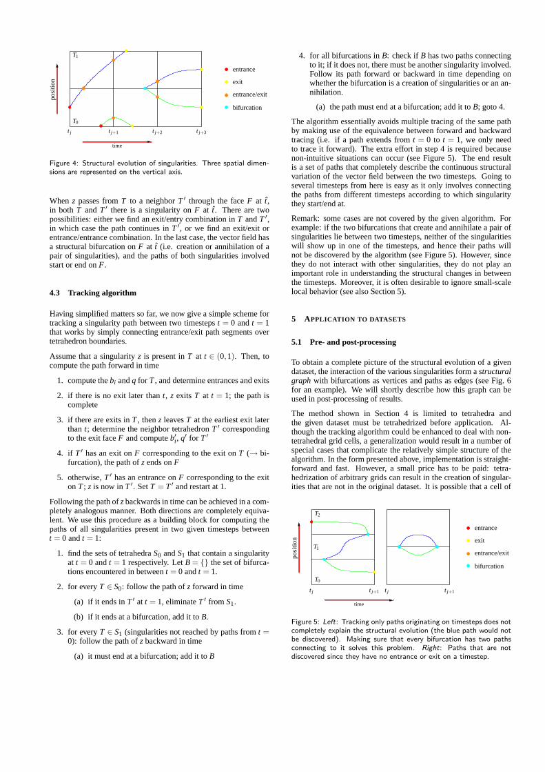
For fixed t ∈ [0,1] there can be at most one singularity inside T(since the field in T is linear), hence we can conclude that if thereis a singularity in T at some t ∈ (0,1), it must either have enteredT at an earlier time 0 < t < t or remained in T since t = 0 (in thiscase we will say that z enters at t = 0). In complete analogy, it musteither exit T at t < t < 1 or remain in T until t = 1 (read z exitsat t = 1). In other words, a singularity path always connects anentrance to an exit, and exits and entrances always come in pairs.Since there cannot be more than one singularity in T at a given time,an entrance is always connected to the closest exit (w.r.t. t).

entrance

exit

entrance/exit

bifurcation

posi

tion

time

T0

T1

t j t j+1 t j+3t j+2

Figure 4: Structural evolution of singularities. Three spatial dimen-sions are represented on the vertical axis.

When z passes from T to a neighbor T ′ through the face F at t,in both T and T ′ there is a singularity on F at t. There are twopossibilities: either we find an exit/entry combination in T and T ′,in which case the path continues in T ′, or we find an exit/exit orentrance/entrance combination. In the last case, the vector field hasa structural bifurcation on F at t (i.e. creation or annihilation of apair of singularities), and the paths of both singularities involvedstart or end on F .

4.3 Tracking algorithm

Having simplified matters so far, we now give a simple scheme fortracking a singularity path between two timesteps t = 0 and t = 1that works by simply connecting entrance/exit path segments overtetrahedron boundaries.

Assume that a singularity z is present in T at t ∈ (0,1). Then, tocompute the path forward in time

1. compute the bi and q for T , and determine entrances and exits

2. if there is no exit later than t, z exits T at t = 1; the path iscomplete

3. if there are exits in T , then z leaves T at the earliest exit laterthan t; determine the neighbor tetrahedron T ′ correspondingto the exit face F and compute b′i, q′ for T ′

4. if T ′ has an exit on F corresponding to the exit on T (→ bi-furcation), the path of z ends on F

5. otherwise, T ′ has an entrance on F corresponding to the exiton T ; z is now in T ′. Set T = T ′ and restart at 1.

Following the path of z backwards in time can be achieved in a com-pletely analogous manner. Both directions are completely equiva-lent. We use this procedure as a building block for computing thepaths of all singularities present in two given timesteps betweent = 0 and t = 1:

1. find the sets of tetrahedra S0 and S1 that contain a singularityat t = 0 and t = 1 respectively. Let B = {} the set of bifurca-tions encountered in between t = 0 and t = 1.

2. for every T ∈ S0: follow the path of z forward in time

(a) if it ends in T ′ at t = 1, eliminate T ′ from S1.

(b) if it ends at a bifurcation, add it to B.

3. for every T ∈ S1 (singularities not reached by paths from t =0): follow the path of z backward in time

(a) it must end at a bifurcation; add it to B

4. for all bifurcations in B: check if B has two paths connectingto it; if it does not, there must be another singularity involved.Follow its path forward or backward in time depending onwhether the bifurcation is a creation of singularities or an an-nihilation.

(a) the path must end at a bifurcation; add it to B; goto 4.

The algorithm essentially avoids multiple tracing of the same pathby making use of the equivalence between forward and backwardtracing (i.e. if a path extends from t = 0 to t = 1, we only needto trace it forward). The extra effort in step 4 is required becausenon-intuitive situations can occur (see Figure 5). The end resultis a set of paths that completely describe the continuous structuralvariation of the vector field between the two timesteps. Going toseveral timesteps from here is easy as it only involves connectingthe paths from different timesteps according to which singularitythey start/end at.

Remark: some cases are not covered by the given algorithm. Forexample: if the two bifurcations that create and annihilate a pair ofsingularities lie between two timesteps, neither of the singularitieswill show up in one of the timesteps, and hence their paths willnot be discovered by the algorithm (see Figure 5). However, sincethey do not interact with other singularities, they do not play animportant role in understanding the structural changes in betweenthe timesteps. Moreover, it is often desirable to ignore small-scalelocal behavior (see also Section 5).

5 APPLICATION TO DATASETS

5.1 Pre- and post-processing

To obtain a complete picture of the structural evolution of a givendataset, the interaction of the various singularities form a structuralgraph with bifurcations as vertices and paths as edges (see Fig. 6for an example). We will shortly describe how this graph can beused in post-processing of results.

The method shown in Section 4 is limited to tetrahedra andthe given dataset must be tetrahedrized before application. Al-though the tracking algorithm could be enhanced to deal with non-tetrahedral grid cells, a generalization would result in a number ofspecial cases that complicate the relatively simple structure of thealgorithm. In the form presented above, implementation is straight-forward and fast. However, a small price has to be paid: tetra-hedrization of arbitrary grids can result in the creation of singular-ities that are not in the original dataset. It is possible that a cell of

entrance

exit

entrance/exit

bifurcation

posi

tion

time

T0

T1

T2

t j+1t j t jt j+1

Figure 5: Left: Tracking only paths originating on timesteps does notcompletely explain the structural evolution (the blue path would notbe discovered). Making sure that every bifurcation has two pathsconnecting to it solves this problem. Right: Paths that are notdiscovered since they have no entrance or exit on a timestep.

index 0 is split up in such a way that the resulting tetrahedra havenon-vanishing index. These “artificial” singularities do not pose aproblem, since they are always created in pairs and usually only lastfor a very brief amount of time.

Numerical datasets are often subject to noise, especially if the com-putations involve some kind of differentiation. It is common prac-tice to apply smoothing operators to datasets in order to undo someof the damage done by previous computations. Commonly, numer-ical noise reflects in short-lived pairs of artificial singularities thatexist in isolation and are not part of the dataset’s structural evolu-tion over time. It can also occur that a path is “interrupted” by a pairof artificial bifurcations that enclose a path segment of very shortduration (Fig. 5 (left) gives an example).

What seems a drawback at first can be turned into an advantage:instead of smoothing the dataset we filter the resulting set of singu-larity paths by removing paths that last less than e.g. one timestep.Filtering can be applied on the structural graph directly and canbe implemented in an efficient way by first removing edges thatrepresent paths with short duration and successively removing allisolated vertices. In our experiments, we found this method to bevery effective in treating noisy datasets. It turns out that conven-tional smoothing does not significantly reduce the number of artifi-cial singularities. It however affects the structure of the dataset insuch a way that the structural evolution is obscured or changed (thisis especially true for minimum/maximum tracking as described inthe next paragraph).

5.2 Tracking of minima and maxima

The presented algorithm is concerned with tracking singularities invector fields. By applying the above approach to gradient fieldsof scalar quantities, we are able to track the evolution of minimaand maxima throughout time through following the paths of the as-sociated singularities in the gradient fields. The algorithm can bedirectly applied to this modified problem. The resulting structuralgraph can then be filtered to only include paths of suitable singu-larities, i.e. attracting and repelling nodes. Note that while minimaand maxima do not necessarily appear in pairs, they are still createdand destroyed at bifurcations in the structural evolution. Althoughe.g. saddle points in the gradient field might have some physicalmeaning as well, we did not consider them in our examples (seeSection 6).

5.3 Visualization

The structural evolution of a vector field is basically a graph whosevertices have a total of four coordinates (3D space + 1D time).Representing the paths of singularities in three-space directly turnsout to be non-intuitive, and adding temporal information to thepresented locations via color-coding or animation does not help.Therefore, we approach the problem by first reducing the dimen-sion from four to two by a change of coordinates.

In one of our examples (cf. 6), the dataset is highly rotation sym-metric and singularities appear and move on the symmetry axisonly. Their complete evolution is then easily represented in a 2ddiagram. However, the other example is much more intricate, andthere is no canonical axis to represent the movement of the singu-larities. If the positions of all singularities at all times are takeninto account, then we are able to determine the principal spatialdirection and the common center of their movement by evaluatingthe zeroth and first order terms of the corresponding principal com-ponent analysis. This provides a suitable spatial coordinate along

which to describe the location of singularities. For more compli-cated datasets, higher order terms of the PCA and interpolation canbe drawn upon to generate a curved coordinate. The resulting two-dimensional diagrams quickly enable the viewer to discover keypoints in the structural evolution that can then be analyzed in detailwith other methods.

6 RESULTS

We have applied our algorithm to two different time-dependentdatasets of CFD simulations performed by the German AerospaceCenter (DLR)/Gottingen using their TAU code. All datasets takethe form of a velocity field provided on the vertices of an unstruc-tured grid consisting of tetrahedra, pyramids and prisms. Althoughthe simulations are based on problems that show some degree ofsymmetry, the computation was performed on the full domain.While the can dataset retains the symmetry of the original prob-lem, the delta wing dataset shows increasingly different behavioron both sides of the wing as time passes.

It is already known that vortex breakdown is associated with the oc-currence of (pairwise) stagnation points, therefore we have appliedthe tracking algorithm to the velocity fields first. Furthermore, thereare speculations that both acceleration and helicity play an impor-tant role in this context. We have computed these fields for thosedatasets and applied tracking to them as well, in the case of helic-ity (which is a scalar quantity) minimum tracking was performed(as described in Section 5). Since these computations involved tak-ing derivatives of the original velocity fields, we observed strongnumerical noise in both helicity and acceleration yielding many ar-tificial singularities. Using the structural graph filtering method de-scribed in Section 5 we were still able to obtain meaningful results.

The tracking algorithm itself is of linear complexity in both thenumber of singularities and the number of timesteps. The mosttime-intensive part is the pre-computation of all singularities in atimestep, for which each cell has to be considered individually. Ifthis information is already given, the running times for our exam-ples are on the order of seconds. Since the algorithm only needstwo successive timesteps to do its work, it is possible to integrateit directly into the CFD simulation. The structural graph for alltimesteps can then be completed in post-processing. This wouldalso allow for online supervision of simulations that are still inprogress. We will now detail the results for both datasets.

6.1 Can dataset

The simulation describes a can filled with a highly viscous fluidthat is accelerated by rotation of the lower lid. The rotational speedvaries over time, leading to breakdown of the central vortex thatcovers the symmetry axis of the can. Due to the high viscosity ofthe fluid and the high degree of symmetry the velocity field is ofvery good numerical quality. This dataset is very close to beinga standard model of vortex breakdown. It consists of about 5000timesteps on a grid with approx. 4.4 million tetrahedra after de-composition.

The results are of almost analytical quality (see Figure 6). The sim-ulation actually shows two occurrences of vortex breakdown (andtwo corresponding pairs of stagnation points) and it is interesting toobserve how primary and secondary vortex breakdown successivelymerge and re-split. Acceleration zeros and helicity minima show astrong correlation with the onset of the breakdown process and thebifurcation that creates the two stagnation points. Before our anal-ysis of the dataset, this correlation was not known. It is also obvi-

ous that the structural graph serves as a kind of “directory” for thedifferent timesteps by indicating interesting phenomena. Throughthis, relevant timesteps can be identified quickly and reliably.

6.2 Delta Wing dataset

In order to study vortex breakdown in aviation, an unsteady simu-lation of a delta wing configuration was performed. The angle ofattack is increased over time, and the primary vortices eventuallyexhibit breakdown. The simulation totals 1000 time steps that de-scribe the formation and breakdown of the primary vortices overtime. The grid consists of about 18 million tetrahedra after decom-position. The dataset is somewhat noisy in a numerical sense sincethe resolution is still too low in some of the more interesting partsof the dataset (this is especially true for the vortex breakdown re-gions). Figure 7 provides an overview showing stream surfaces thatwrap around the primary vortices above the wing (red and blue).Asymmetric breakdown is clearly visible.

We have used our method on two regions in the dataset that corre-spond to breakdown on both sides of the wing. After the coordi-nate transformation (see also Section 5), the structural graph of theright region (cf. Figure 8) clearly shows the evolution of the stag-nation points as they move towards the wing. Again, accelerationzeros and a helicity minimum seem to play a role in formation ofbreakdown, although the correlation is not as obvious as in the candataset. This is, in part, to be blamed upon the lack in resolutionand the resulting numerical instability of differentiation. Filteringof the structural graph for the helicity gradient field (whose com-putation involves a second spatial derivative) reduced the numberof meaningful paths from roughly 1.000 to 4, effectively eliminat-ing all artificial singularities. The left region is even more chaotic,and it is clearly visible how the stagnation points begin to oscil-late and disappear around timestep 730, to be followed by whatappears to be a sequence of short-lasting vortex breakdowns in dif-ferent places. In this case, the structure graph helps in groupingthe velocity field singularities that would otherwise just be isolatedsingularities in the field without any context. Figure 7 gives a directcomparison between the evolution of stagnation points on the leftand right sides and the corresponding flow structures (displayed bystream surfaces). While the behavior is almost similar in the begin-ning, the left side quickly deteriorates. Again, the structure graphcan provide for a direct qualitative comparison that is very hard toachieve by other means (e.g. streamlines or surfaces).

7 CONCLUSION

The objective of the work presented in this paper was to determinethe structural evolution of certain types of complex time-dependentCFD datasets. First, we have presented a number of theoretical re-sults about the Poincare index in three spatial dimensions. It is anextremely powerful yet intuitively geometric concept of describingsingularities of 3D vector fields and the laws they must obey undertime-varying circumstances. Considering the restrictions imposedby tetrahedral grids with piecewise linear interpolation in space andtime, we were able to give a robust and straightforward algorithmto the intended purpose. By providing a temporal overview of thedataset using the structural graph that is built from singularity paths,it is possible to quickly determine points of interest in large datasetswith many timesteps. Furthermore, the method has already provenuseful in the analysis of two datasets where the flow exhibits vor-tex breakdown. Since understanding of this phenomenon is stillincomplete from a fluid mechanical point of view, we believe that

the uncovered interrelations of various quantities can be an impor-tant step towards a complete explanation. Here, visualization canshow its strength by giving new impulses in fluid mechanics.

There is however some space for improvement on the presentedmaterial. The tracking algorithm could be extended to deal withtrilinear interpolation to make possible the treatment of CFD gridsdirectly without the need for prior tetrahedrization. So far, singu-larities have not played a significant role in the analysis of CFDdatasets; this has changed with the advent of simulations that areable to resolve very complex flow patterns. If a more completepicture of a given flow can be obtained via the structural graph,the detection of certain types of flow behavior could be automatedbased on the graph. With efforts underway to automatically op-timize the geometries of e.g. aircraft to exclude undesired effects,the structural graph could provide a robust criterion to indicate theirpresence. Vortex breakdown serves as a prime example.

ACKNOWLEDGEMENTS

Foremost, the authors would like to thank Markus Rutten from DLRGottingen for close collaboration and insightful remarks. He kindlyprovided the datasets considered here. Our gratitude also extendsto all members of the FAnToM project at the University of Kaiser-slautern for their implementation efforts. This work was partly sup-ported by DFG grants HA 1491/15-4 and HA 1491/15-5.

REFERENCES

[1] D. Bauer and R. Peikert. Vortex tracking in scale-space. In DataVisualization 2002. Proc. VisSym ’02, 2002.

[2] J. Chen, D. Silver, and L. Jiang. The feature tree: Visualizing featuretracking in distributed amr datasets. In IEEE Symposium on Paralleland Large-Data Visualization and Graphics, 2003.

[3] J. Guckenheimer and P. Holmes. Nonlinear Oscillations, DynamicalSystems, and Bifurcations of Vector Fields. Springer-Verlag, 1983.

[4] J. L. Helman and L. Hesselink. Visualizing Vector Field Topology inFluid Flows. IEEE Computer Graphics and Applications, 11(3):36–46, May 1991.

[5] D. Hestenes and G. Sobzyk. Clifford Algebra to Geometric Calculus.D. Reidel Publishing Company, 1984.

[6] D. N. Kenwright and R. Haimes. Vortex Identification - Applicationsin Aerodynamics: A Case Study. In R. Yagel and H. Hagen, editors,IEEE Visualization ’97, pages 413–416, Los Alamitos, CA, 1997.

[7] K. Mahrous, J. Bennet, G. Scheuermann, B. Hamann, and K. I. Joy.Topological segmentation in three-dimensional vector fields. IEEETransactions on Visualization and Computer Graphics, 10(2):198–205, 2004.

[8] T. Mullin, J. J. Kobine, S. J. Tavener, and K. A. Cliffe. On the creationof stagnation points near straight and sloped walls. Physics of Fluids,12(2), 2000.

[9] R. Samtaney, D. Silver, N. Zabusky, and J. Cao. Visualizing featuresand tracking their evolution. IEEE Computer, 27(2):20 – 27, 1994.

[10] D. Silver and X. Wang. Tracking and visualizing turbulent 3d fea-tures. IEEE Transactions on Visualization and Computer Graphics,3(2), 1997.

[11] H. Theisel, T. Weinkauf, H.-C. Hege, and H.-P. Seidel. Saddle connec-tors - an approach to visualizing the topological skeleton of complex3d vector fields. In IEEE Visualization ’03, 2003.

[12] X. Tricoche, T. Wischgoll, G. Scheuermann, and H. Hagen. Topol-ogy tracking for the visualization of time-dependent two-dimensionalflows. Computers & Graphics, 26(2):249 – 257, 2002.

[13] C. Weigle and D. C. Banks. Extracting iso-valued features in 4-dimensional scalar fields. 1998.

0 0.2 0.4 0.6 0.8 1

758

1602

1888

2458

2968

4925

singularity position on principal axis

times

tep

stagnation pointhelicity min.acceleration zero

primary vortex breakdown

secondary vortex breakdown

structural evolution timestep 1700 timestep 4400

Figure 6: Left: Structural graph of the can dataset. The green paths represent the stagnation points in the velocity field. Primary andsecondary breakdown each create a pair of stagnation points. Around timestep 1888, the two phenomena join, only to re-split at timestep 2458and successively decay. The blue and orange paths belong to helicity minima and acceleration zeros. Note the strong interrelation between thethree quantities. Right: Two snapshots from the can dataset. Separation stream surfaces are started at the singularity positions. Timestep1700 shows both breakdowns, whereas the second breakdown has already vanished in timestep 4000 and the first breakdown shows the typical“mushroom” structure.

1 1.5

595

singularity position

times

tep

stagnation pointshelicity min.acceleration zeros

1 1.5

597

723

singularity position

times

tep

stagnation pointshelicity min.acceleration zeros

right breakdown left breakdown

Figure 7: Left: Overview of the delta wing dataset with its two primary vortices above the wings. Stream surfaces wrap around the vorticesand are eventually distorted by vortex breakdown. Note the asymmetrical breakdown structure. Right: Structural graphs for right and leftbreakdown. Again a connection between various quantities involved in vortex breakdown can be observed for the right breakdown. In the leftbreakdown, several oscillating breakdown structures are visible in the later timesteps.

1 1.5540

620

700

780

860

singularity position

times

tep

stagnation points leftstagnation points right

structural evolution left vs. right timestep 730 (right vortex breakdown) timestep 730 (left vortex breakdown)

Figure 8: Comparison of right and left breakdown structures. Left: The combined structural graphs make an intuitive comparison possible.Right: transparent stream surfaces show the distortion of the flow and the intricate flow patterns that make analysis difficult. The left breakdowndoes not show the usual breakdown structure and consists of several smaller and independent breakdowns.