Tracking in magnetic fields

Advanced FLUKA Course

2

Magnetic field tracking in FLUKA

FLUKA allows for tracking in arbitrarily complex magnetic fields.Magnetic field tracking is performed by iterations until a givenaccuracy when crossing a boundary is achieved.Meaningful user input is required when setting up the parameters defining the tracking accuracy.Furthermore, when tracking in magnetic fields FLUKA accounts for: The precession of the mcs final direction around the particle direction:

this is critical in order to preserve the various correlations embeddedin the FLUKA advanced MCS algorithm

The precession of a (possible) particle polarization around its directionof motion: this matters only when polarization of charged particles is aissue (mostly for muons in Fluka)

The decrease of the particle momentum due to energy losses along agiven step and hence the corresponding decrease of its curvatureradius. Since FLUKA allows for fairly large (up to 20%) fractionalenergy losses per step, this correction is important in order to preventexcessive tracking inaccuracies to build up, or force to use very smallsteps

3

Magnetic field tracking in FLUKA

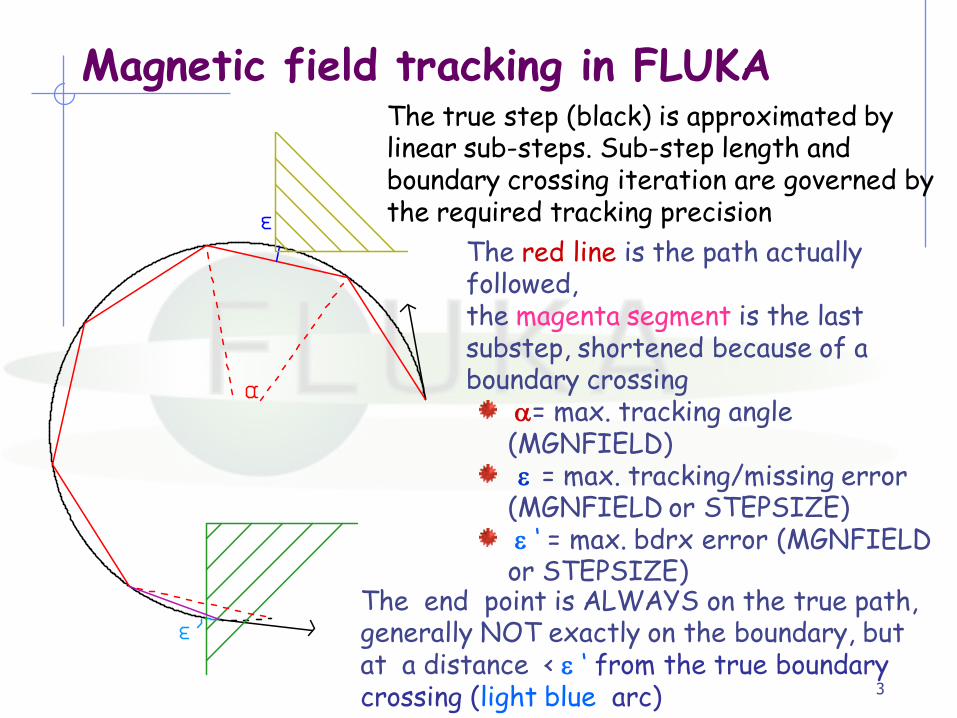
The red line is the path actually followed, the magenta segment is the last substep, shortened because of a boundary crossing

= max. tracking angle (MGNFIELD) = max. tracking/missing error

(MGNFIELD or STEPSIZE) „ = max. bdrx error (MGNFIELD or STEPSIZE)

The true step (black) is approximated by linear sub-steps. Sub-step length and boundary crossing iteration are governed by the required tracking precision

The end point is ALWAYS on the true path,generally NOT exactly on the boundary, but at a distance < „ from the true boundary crossing (light blue arc)

4

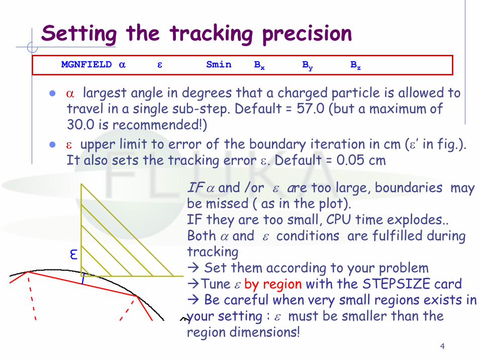
Setting the tracking precision

largest angle in degrees that a charged particle is allowed to travel in a single sub-step. Default = 57.0 (but a maximum of 30.0 is recommended!)

upper limit to error of the boundary iteration in cm (‟ in fig.). It also sets the tracking error . Default = 0.05 cm

MGNFIELD Smin Bx By Bz

IF and /or are too large, boundaries may be missed ( as in the plot). IF they are too small, CPU time explodes..Both and conditions are fulfilled during tracking Set them according to your problemTune by region with the STEPSIZE card Be careful when very small regions exists in your setting : must be smaller than the region dimensions!

5

Setting the tracking precision

Smin minimum sub-step length. If the radius of curvature is so small that the maximum sub-step compatible with is smaller than Smin, then the condition on is overridden. It avoids endless tracking of spiraling low energy particles. Default = 0.1 cm

MGNFIELD Smin Bx By Bz

Particle 1: the sub-step corresponding to is > Smin -> acceptParticle 2: the sub-step corresponding to is < Smin -> increase

Smin can be set by region with the STEPSIZE card

6

Setting precision by region

Smin: (if what(1)>0) minimum step size in cm Overrides MGNFIELD if larger than its setting.

(if what(1)<0) : max error on the location of intersection with boundary. The possibility to have different “precision” in different

regions allows to save cpu time

Smax : max step size in cm. Default:100000. cm for a region without mag field, 10 cm with mag field. Smax can be useful for instance for large vacuum regions

with relatively low magnetic field It should not be used for general step control, use

EMFFIX, FLUKAFIX if needed

STEPSIZE Smin/ Smax Reg1 Reg2 Step

7

Possible loops in mag.fields

Although rare, it is PHYSICALLY possible that a particle loops for ever ( or for a very long time). Imagine a stable particle generated perpendicularly to a uniform B in a large enough vacuum region: it will stay on a circular orbit forever !

Suppose now that the orbit enters in a non-vacuum region (here we can at least loose energy..) but the boundary is missed due to insufficient precision. This results again in a never-ending loop.

Luckily, it almost never happens. Almost.

8

The magfld.f user routineThis routine allows to define arbitrarily complex magnetic fields:

( uniform fields can be defined trough the MGNFIELD card)

SUBROUTINE MAGFLD ( X, Y, Z, BTX, BTY, BTZ, B, NREG, IDISC)

. Input variables:

x,y,z = current position

nreg = current region

Output variables:

btx,bty,btz = cosines of the magn. field vector

B = magnetic field intensity (Tesla)

idisc = set to 1 if the particle has to be discarded

All floating point variables are double precision ones!

BTX, BTY, BTZ must be normalized to 1 in double precision

Magfld .f is called only for regions where a magnetic field has been declared through ASSIGNMAT

Example: magnetic field in CNGS

Cern Neutrino to Gran Sasso

The two magnetic lenses (blue in the sketch) align positive mesons towards the Decay tunnel, so that neutrinos from the decay are directed to Gran Sasso, 730~km awayNegative mesons are deflected awayThe lenses have a finite energy/angle acceptance

Example : the magfld.f routine

Magnetic field intensity in the CNGS horn

A cuurent ≈150kA, pulsed, circulates through the InnerandOuterconductorsThe field is toroidal, B1/R

magfld: exampleSUBROUTINE MAGFLD ( X, Y, Z, BTX, BTY, BTZ, B, NREG, IDISC )

INCLUDE '(DBLPRC)'INCLUDE '(DIMPAR)'INCLUDE '(IOUNIT)„

INCLUDE '(NUBEAM)'

IF ( NREG .EQ. NRHORN ) THENRRR = SQRT ( X**2 + Y**2 )BTX =-Y / RRRBTY = X / RRRBTZ = ZERZERB = 2.D-07 * CURHOR / 1.D-02 / RRR

END IF

In this case, the cosines are automatically normalized. Otherwise, user MUST ensure thatBTX**2+BTY**2+BTZ**1=ONEONE

USEFUL TIPThis is a user defined include file, containing for example COMMON /NUBEAM/ CURHORN, NRHORN, ……

It can be initialized in a custom usrini.f user routine, so that parameters can be easily changed in the input file

This gives a versor radiusin a plane z axis

B intensity depending on R and current

Standard FLUKA includes : KEEP THEM

magfld: example contndDifferent fields in different regions:

IF ( NREG .EQ. NRHORN ) THEN……

ELSE IF ( NREG .EQ. NRSOLE ) THENBTX = ZERZERBTY = ZERZERBTZ = ONEONEB = SOLEB

ELSE IF ( NREG .EQ. NRMAP ) THENCALL GETMAP ( X, Y, Z, BTX, BTY, BTZ, B)

ELSEWRITE ( LUNOUT, *) „MGFLD, WHY HERE ?WRITE ( LUNOUT, *) NREG‟STOP

END IF

This gives a perfect solenoid field

Intensity calculated at initialization

Add a bit of protection.

Get values from field map

The user can add more routines, they have to be included in the linking procedureAlways :

include the three standard FLUKA INCLUDEs use FLUKA defined constants and particle properties for consistency

Possible, not explained here : call C routines

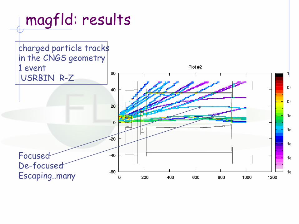
magfld: results

charged particle tracks in the CNGS geometry1 eventUSRBIN R-Z

FocusedDe-focusedEscaping..many

The user initialization routines usrglo.f called before all initialization, if a USRGCALL card is

issued

usrini.f called after all initialization, if a USRICALL card isissued

usrein.f called at each event, before the showering of an event is started, but after the source particles of that event have been already loaded on the stack. No card is needed

Very useful to initialize and propagate variables common to other user routines

Associated OUTPUT routines:

usrout.f called at the end of the run if USROCALL is present

usreout.f called at the end of each event , no card needed

15

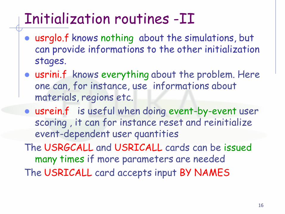
Initialization routines -II usrglo.f knows nothing about the simulations, but

can provide informations to the other initialization stages.

usrini.f knows everything about the problem. Here one can, for instance, use informations about materials, regions etc.

usrein.f is useful when doing event-by-event user scoring , it can for instance reset and reinitialize event-dependent user quantities

The USRGCALL and USRICALL cards can be issued many times if more parameters are needed

The USRICALL card accepts input BY NAMES

16

usrini.f :example

17

SUBROUTINE USRINI ( WHAT, SDUM )

INCLUDE '(DBLPRC)'INCLUDE '(DIMPAR)'INCLUDE '(IOUNIT)„

…..DIMENSION WHAT (6)CHARACTER SDUM*8

….CHARACTER MAPFILE(8) INCLUDE '(NUBEAM)„

IF ( SDUM .EQ. 'HORNREFL' ) THENNRHORN = WHAT (1)CURHORN = WHAT (2)

ELSE IF (SDUM .EQ. „SOLENOID„) THENSOLEB = WHAT (2)NRSOLE = WHAT(1)

contnd

Default declarations

Here we store our variables

Here we initialize region numbersAnd parameters for the magfld.froutine

usrini.f: example contnd

18

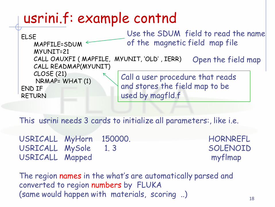
ELSEMAPFILE=SDUMMYUNIT=21CALL OAUXFI ( MAPFILE, MYUNIT, „OLD‟ , IERR)CALL READMAP(MYUNIT)CLOSE (21)NRMAP= WHAT (1)

END IFRETURN

Use the SDUM field to read the name of the magnetic field map file

Open the field map

Call a user procedure that reads and stores the field map to be used by magfld.f

This usrini needs 3 cards to initialize all parameters:, like i.e.

USRICALL MyHorn 150000. HORNREFLUSRICALL MySole 1. 3 SOLENOIDUSRICALL Mapped myflmap

The region names in the what‟s are automatically parsed and converted to region numbers by FLUKA(same would happen with materials, scoring ..)

Roto-translation routines:

19

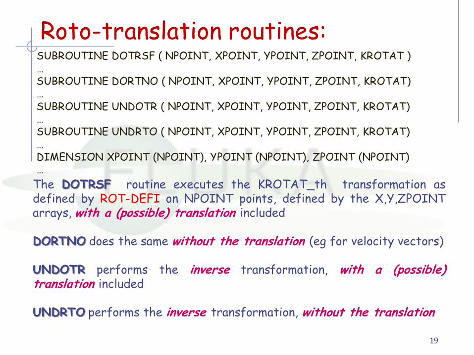
The DOTRSF routine executes the KROTAT_th transformation asdefined by ROT-DEFI on NPOINT points, defined by the X,Y,ZPOINTarrays, with a (possible) translation included

DORTNO does the same without the translation (eg for velocity vectors)

UNDOTR performs the inverse transformation, with a (possible)translation included

UNDRTO performs the inverse transformation, without the translation

SUBROUTINE DOTRSF ( NPOINT, XPOINT, YPOINT, ZPOINT, KROTAT )…SUBROUTINE DORTNO ( NPOINT, XPOINT, YPOINT, ZPOINT, KROTAT)…SUBROUTINE UNDOTR ( NPOINT, XPOINT, YPOINT, ZPOINT, KROTAT)…SUBROUTINE UNDRTO ( NPOINT, XPOINT, YPOINT, ZPOINT, KROTAT)…DIMENSION XPOINT (NPOINT), YPOINT (NPOINT), ZPOINT (NPOINT)…

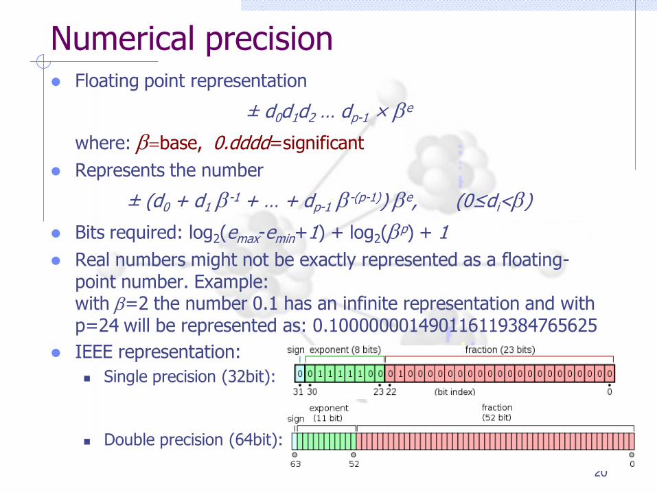
Numerical precision Floating point representation

± d0d1d2 … dp-1 × be

where: b=base, 0.dddd=significant

Represents the number

± (d0 + d1 b-1 + … + dp-1 b-(p-1)) be, (0≤di<b)

Bits required: log2(emax-emin+1) + log2(bp) + 1

Real numbers might not be exactly represented as a floating-point number. Example:with b=2 the number 0.1 has an infinite representation and with p=24 will be represented as: 0.100000001490116119384765625

IEEE representation:

Single precision (32bit):

Double precision (64bit):

20

Floating point: Accuracy Cancellation: subtraction of nearly equal operands may cause

extreme loss of accuracy.

Conversions to integer are not intuitive:converting (63.0/9.0) to integer yields 7,but converting (0.63/0.09) may yield 6.This is because conversions generally truncate rather than round.

Limited exponent range: results might overflow yielding infinity, or underflow yielding a denormal value or zero. If a denormalnumber results, precision will be lost.

Testing for safe division is problematic: Checking that the divisor is not zero does not guarantee that a division will not overflow and yield infinity.

Equality test is problematic: Two computational sequences that are mathematically equal may well produce different floating-point values. Programmers often perform comparisons within some tolerance

21

Minimizing Accuracy Problems Use double precision whenever possible.

Small errors in floating-point arithmetic can grow when mathematical algorithms perform operations an enormous number of times. e.g. matrix inversion, eigenvalues…

Expectations from mathematics may not be realized in the field of floating-point computation. e.g. sin2q+cos2q = 1.

Always replace the x2-y2 = (x+y)(x-y)

Equality test should be avoided: replace with "fuzzy" comparisons (if (abs(x-y) < epsilon) ...)

Adding a large number of numbers can lead to loss of significance, use Kahan algorithm instead

For the quadratic formula use either

or

when b2>>4ac, then √(b2-4ac)≈|b| therefore will introduce cancelation

22

a

acbb

2

42

acbb

c

4

2

2

23

END

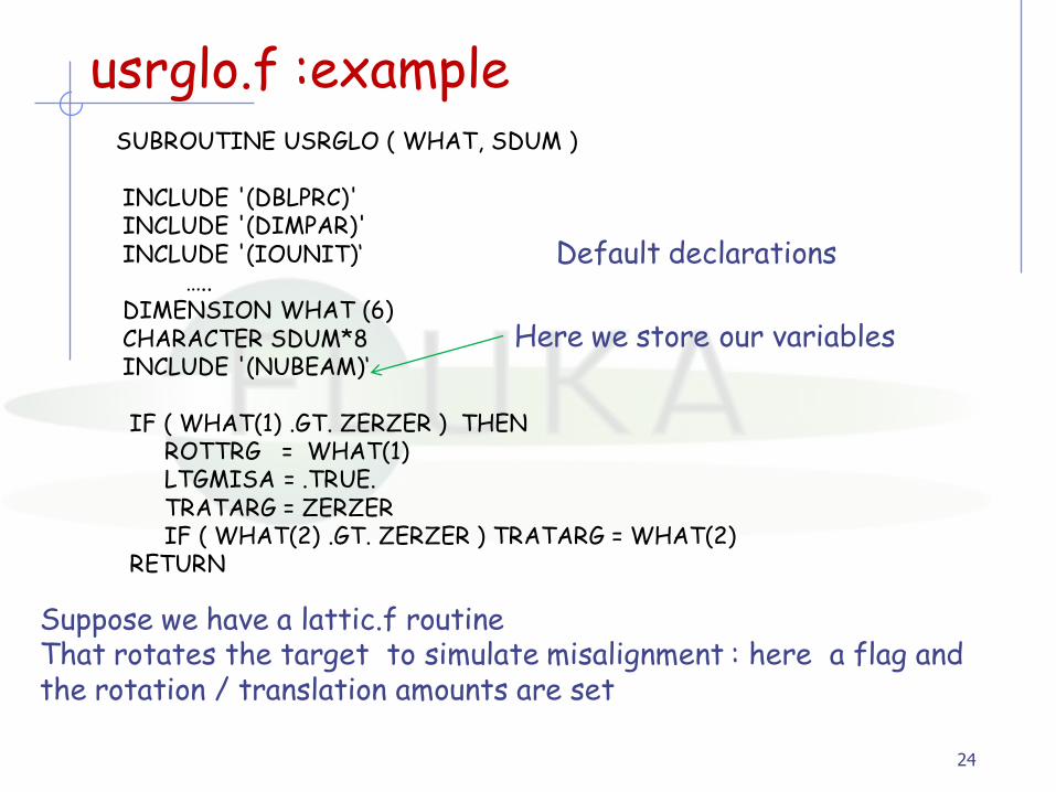
usrglo.f :example

24

SUBROUTINE USRGLO ( WHAT, SDUM )

INCLUDE '(DBLPRC)'INCLUDE '(DIMPAR)'INCLUDE '(IOUNIT)„

…..DIMENSION WHAT (6)CHARACTER SDUM*8INCLUDE '(NUBEAM)„

IF ( WHAT(1) .GT. ZERZER ) THENROTTRG = WHAT(1)LTGMISA = .TRUE.TRATARG = ZERZERIF ( WHAT(2) .GT. ZERZER ) TRATARG = WHAT(2)

RETURN

Default declarations

Here we store our variables

Suppose we have a lattic.f routine That rotates the target to simulate misalignment : here a flag and the rotation / translation amounts are set