TRACKING EDGES, CORNERS AND VERTICES

IN AN IMAGE

PETER HALL PEIHUA QIU

Centre for Mathematics and its Applications School of Statistics

Australian National University University of Minnesota

CHRISTIAN RAU

Department of Mathematics

Hong Kong Baptist University

23 January 2007

ABSTRACT. In a range of imaging problems, particularly those where the imagesare of man-made objects, edges join at points which comprise three or more distinctboundaries between textures. In such cases the set of edges in the plane forms whata mathematician would call a planar graph. Smooth edges in the graph meet oneanother at junctions, called “vertices”, the “degrees” of which denote the respectivenumbers of edges that join there. Conventional image reconstruction methods donot always draw clear distinctions among different degrees of junction, however. Insuch cases the algorithm is, in a sense, too locally adaptive; it inserts junctionswithout checking more globally to determine whether another configuration mightbe more suitable. In this paper we suggest an alternative approach to edge re-construction, which combines a junction classification step with an edge-trackingroutine. The algorithm still makes its decisions locally, so that the method retainsan adaptive character. However, the fact that it focuses specifically on estimat-ing the degree of a junction means that it is relatively unlikely to insert multiplelow-degree junctions when evidence in the data supports the existence of a singlehigh-degree junction. Numerical and theoretical properties of the method are ex-plored, and theoretical optimality is discussed. The technique is based on localleast-squares, or local likelihood in the case of Gaussian data. This feature, and thefact that the algorithm takes a tracking approach which does not require analysisof the full spatial dataset, mean that it is relatively simple to implement.

Key words. Boundary estimation, edge detection, edge representation, image pro-cessing, image segmentation, kernel methods, local least squares, local likelihood,nonparametric curve estimation, planar graph, spatial statistics.

Short Title. Edge, corner and vertex tracking.

1. Introduction

Edges are critical features in many important applications of imaging. An edge

often indicates the boundary of an object in the field of view. This extremity can

provide crucial information about the object, sometimes more important than its

“texture” (e.g. its grey shade or its colour). Not surprisingly, some of the earliest

methods for image enhancement focused on delineating edges, for example by adding

a multiple of the Laplacian back onto the image from which it was computed.

In many contemporary applications of image analysis a more accurate, and

more explicit, estimate of the edge is required, often after part of the edge has been

identified. One wishes to start an edge estimator at a given point that we believe is

close to the edge, and follow the edge through places where it splits into two or more

edges, tracking it up each branch, as well as following it in the reverse direction,

away from the starting point. Edge-splitting is very commonly encountered in real

images; a simple example arises in a non-orthogonal view of a cube, where a corner

of the cube is represented in the planar image by three edges converging at a point.

The angles the edges make to one another in the image depend on the position from

which the cube is viewed. Making decisions about the number of edges into which a

tracked edge splits, and successfully following each of these, is an intrinsically more

difficult problem than estimating a smooth edge from spatial data, or tracking a

smooth edge that does not have any junctions.

We suggest a tracking-based solution to the problem, founded on computing el-

ementary local-likelihoods at discrete points along a piecewise-linear edge estimate.

The points are uniquely determined by an algorithm for defining the piecewise-linear

steps; the local likelihoods are produced by elementary local-linear approximations

to the texture surface, under the temporary assumption of Gaussian noise; and

the results of each likelihood analysis dictate whether the edge we are tracking is

smooth in the neighbourhood of that point, or whether it splits into two or more

edges. In the latter case an estimate of the number of edges is also given by ele-

mentary likelihood analysis. Since the likelihood is constructed under a Gaussian

assumption then the method is equivalently based on local least-squares.

The edge-splitting models can be quite general, however. In particular, the

edges might meet at arbitrary angles at a point, or their junction may be more

narrowly defined. For example, a “T-intersection” model for three edges meeting

2

at a point, with two of the edges collinear, is readily included in the likelihood

analysis, as are many others. The technique is equally appropriate for problems of

image analysis and for nonparametric regression in the case of surfaces with complex

fault-type discontinuities.

An image can be represented abstractly, and globally, as a function f from

the plane IR2 to d-variate space IRd, where the value of f in the jth coordinate

represents the grey-shade at the jth frequency or wavelength. For example, in

a naive model for a colour image the number of components would be d = 3,

representing the three primary colours. In remote-sensing applications the value

of d can be relatively large. For clarity and simplicity we shall treat only the case

d = 1, noting that methodology is similar in other cases.

For either d = 1 or d ≥ 2, and despite the fact that the abstract model is defined

in the continuum, we of course have only discrete data on the model, with the x

variables restricted to a regular grid or, in the case of some statistical applications,

to a stochastic point process in the plane. An example of the latter is undersea

sampling, for example to determine water temperature. (Sea temperature gradients

can be so steep that temperature can be interpreted as having discontinuities.)

Here it is usually impossible to confine the spatial explanatory variables to a grid.

However, in either case the algorithm we suggest is the same.

Taking d = 1 for definiteness, the function f is assumed to be a smooth (e.g. dif-

ferentiable) function of x ∈ IR2, except for the presence of fault-type discontinuities

along a network of lines in the plane, and x is a point in that plane. The fault

lines, which represent the edges, form a planar graph G in which the edges are,

appropriately, represented as graph-theoretic edges, and the points at which edges

join are vertices of the graph. The number of edges that join at a particular point

is that vertex’s graph-theoretic degree. This abstraction will form the basis of our

model for edges in images. We shall develop an algorithm which uses discrete noisy

data on textures (that is, on the values taken by f at points x not on G) to estimate

the locations and degrees of all vertices, and the locations of edges linking vertices.

Recent monograph-length accounts of computer vision include those of Jahne

& Haussecker (2000), Forsythe & Ponce (2003), Hartley & Zisserman (2003) and

Qiu (2005). Earlier monographs on computer vision and image analysis, paying

particular attention to edge detection, include those by Gonzalez & Woods (1992),

3

Haralick & Shapiro (1992), Morel & Solimini (1995) and Parker (1997). Wavelet-

based methods are discussed by Mallat (1999). Existing approaches to edge detec-

tion in computer vision usually begin with a pre-processing step, addressing issues

such as illumination correction and noise suppression, before attempting to track

the edge. By way of contrast, the approach taken in the present paper derives edge

maps directly from the current data, in a single algorithm, reflecting statistical ar-

guments that it is optimal to fit simultaneously all explanatory effects (illumination

angle, noise, edges etc). The output of conventional edge detectors can be quite

poor in the neighbourhood of corners and junctions, because those features of edges

are not explicitly accommodated by standard edge models. Moreover, much of the

literature on edge detection is rather informal, with relatively little rigorous theo-

retical backing. The present paper avoids these pitfalls through using edge models

which incorporate corners and junctions, and by providing a theoretical account of

performance.

Among recent contributions to smooth edge estimation based on spatial data

we mention those of Sinha & Schunck (1992), Bhandarkar et al. (1994), Yi & Chel-

berg (1995), Qiu & Yandell (1997, 1998), Miyajima & Mukawa (1998), Qiu (1998),

Bhandarkar & Zeng (1999) and Pedersini et al. (2000). O’Sullivan & Qian (1994),

Chan et al. (1996), Hall & Rau (2000) and Hall et al. (2001) have suggested methods

for fault-line tracking. Techniques proposed in the context of Markov random field

models include those for fitting predetermined curved objects to boundaries, and

for imputing line patterns; see e.g. Li (1995a, pp. 119, 177; 1995b; 2000), Achour et

al. (2001), Kang & Kweon (2001), Kang & Roh (2001) and Park & Kang (2001).

2. Methodology

2.1. Features of a planar graph

A planar graph, G, is a set of smooth planar curves, called edges, joined together

at points called vertices. A vertex of degree k ≥ 1 in G is a point from which

radiate just k edges. We shall assume for simplicity that no two of these edges

have the same orientation at the vertex, although this restriction can be removed;

see subsection 2.4 for discussion. The main virtue of this “sharp vertex” condition

is that it removes the possibility that multiple edges join vertices in a collinear

way, i.e. that their tangents there have the same orientations. Our method would

produce statistically consistent vertex estimators in this case, but the estimators

4

would not enjoy the convergence rates given in section 4.

The case k = 2, where just two edges meet at a vertex, is that of a corner. In

this setting the “sharp vertex” assumption removes the degenerate case, where the

angle between the two edges equals 0 or π, and so ensures that the corner has the

character that it would in popular parlance. Of course, when k = 2 but the tangents

meet at an angle that is very close to 0 or π, the corner may be relatively difficult

to detect, and may be missed altogether unless the level of noise is relatively low.

Analogously, in the context of hypothesis testing, if the null hypothesis is false but

the alternative hypothesis is close to the null, the power of the test will be relatively

low, and the alternative may not be detected.

A vertex of degree 3 or more, i.e. for which k ≥ 3, will be called a knot. An

edge in G will be assumed to be a segment of a planar curve of bounded curvature

which joins two vertices. (The “sharp vertex” assumption removes degeneracy, by

implying that the edge contains no vertices other than those at its ends.) The graph

will be assumed to be connected, to contain only a finite number of vertices (and,

consequently, only a finite number of edges), and to have finite total length. All

graphs that we shall consider will be assumed to have these properties, which we

shall denote by (G). The assumption of connectivity serves only to ensure that we

can track G in its entirety by starting at a single point.

Note that each edge ends in a vertex. In particular, a vertex of degree 1 is the

endpoint of an edge which, at that end, is linked to no other edge. Figure 1 shows

a graph, G, having vertices of differing degrees.

Place Figure 1 here, please

2.2. Global model for surfaces

Given a graph G satisfying (G), let f be a function from IR2 to IR such that (a) Gis contained in an open subset, S, of the support of f , (b) all first derivatives of

f are uniformly bounded on S \ G, and (c) for each η > 0 the height of the jump

discontinuity at x ∈ G is bounded away from zero uniformly in points x that are

distant at least η from all vertices of degree 1 in G. (If x is a vertex of degree k ≥ 2

then this assumption is taken to mean that the k limits of f(v), as v → x through

points in any one of the k segments of S \ G that meet at the vertex x, are all

distinct.)

We shall denote these properties by (F). Given a function f satisfying (F), our

5

global model for the surface is defined by y = f(x), x ∈ S. The value of f(x) might

represent the colour, or grey shade, of an image at x. In this case G would denote

the set of sharp boundaries between different colours in the image. Figure 2 depicts,

for a graph G simpler than that in Figure 1, a function f satisfying (F) for this G.

Place Figure 2 here, please

2.3. Local model for surfaces

Let Θ denote the set of all bivariate unit vectors. Our local (linear) model, Mk,

for a surface will resemble the k wedge-shaped slices of a circular cake, the wedges

meeting at a point x0 ∈ IR2. The height of the local surface model, above the plane

IR2, will be taken to have constant value ci on the ith wedge. The model will be used

to approximate a more elaborate surface, such as that described in subsection 2.2,

where surface height has discontinuities along the edges of a graph G of which x0 is

a vertex of degree k, for k ≥ 2.

Specifically, let Mk = Mk(x0, θ1, . . . , θk, c1, . . . , ck), for k ≥ 2, be the surface

defined by y = fk(x), where x ∈ IR2 and fk = fk( · |x0, θ1, . . . , θk, c1, . . . , ck) is

the function that equals ci on the infinite wedge that has its vertex at x0 and its

two straight sides in the directions of θi and θi+1. Each θi ∈ Θ, and we take

θk+1 = θ1. It is assumed that the θi’s are arranged such that passing from θi to

θi+1 involves rotating counterclockwise about the origin, without crossing any other

unit vectors θj . We define fk arbitrarily at x0 and on the infinite rays that point

in directions θ1, . . . , θk.

2.4. Local surface estimators

In this subsection we construct local approximations to the function f , using a

least-squares method with kernel weights. The approximations will be used in

subsection 2.5 to guide an algorithm for tracking, from data, the graph G.

Noisy observations Yi are made of f at points Xi ∈ IR2. Specifically, we record

the values of Yi = f(Xi) + ei, 1 ≤ i ≤ n, where f satisfies (F) and corresponds

to a graph G that satisfies (G), and the errors ei are independent and identically

distributed random variables, independent also of X1, . . . Xn, with zero mean and

finite variance. (The value of n may be infinite, if the process of points Xi covers the

entire plane.) Using the data (Xi, Yi), 1 ≤ i ≤ n, we wish to construct an estimator

of f which respects the vertices of G. In particular, we wish to estimate the number

of vertices of G, and their respective locations and degrees, and to construct an

6

estimator G of G whose vertices have the estimated properties. Our first step is to

construct a sequence of local estimators of f .

To this end, let K denote a kernel function, which we take to be a compactly

supported, bivariate probability density, and let h be a bandwidth. Let fk denote

the function defined in subsection 2.3, and put Ki(x0) = K{(x0 −Xi)/h} and

Sk(x0 | θ1, . . . , θk, c1, . . . , ck) =n∑

i=1

{Yi − fk(Xi |x0, θ1, . . . , θk, c1, . . . , ck)

}2Ki(x0) .

(1)

Then Sk(x0 | θ1, . . . , θk, c1, . . . , ck) is proportional to a negative log-likelihood in the

case where the true function is representable by the local model,

fk(· |x0, θ1, . . . , θk, c1, . . . , ck) ,

in the vicinity of x0, and the data (Xi, Yi) are generated in the form Yi = fk(Xi)+ei,

with the errors ei being Gaussian with zero mean and fixed variance. Of course, the

methodology suggested by these very specialised assumptions is going to be useful

in much more general settings, as we shall show in sections 3 and 4.

Returning to the one-dimensional case we choose θ1, . . . , θk, c1, . . . , ck to min-

imise the sum of squares at (1), and write simply Sk(x0) for the corresponding value

of the left-hand side. The surface defined by y = f(x) is estimated locally, near x0,

as the surface with equation y = fk(x |x0, θ1, . . . , θk, c1, . . . , ck). If the kernel K is

smooth and unimodal, with a uniquely defined mode, then the parameter estimators

are uniquely defined with probability 1.

We take f1 to be the function corresponding to a local linear model for the

surface at a point x0 that is on an edge of G but not a vertex. Thus,

f1(x) = f1(x |x0, θ, c+, c−) ={c+ if x ∈ H+(x0, θ)c− if x ∈ H−(x0, θ) ,

(2)

where H±(x0, θ) are the half-planes on opposite sides of the infinite line that passes

through x0 and is parallel to θ. The function f0, which is simply constant through-

out IR2, corresponds to our zeroth surface model, which is flat everywhere. The

local surface model Mk, represented by the equation y = fk(x), will be said to be

of degree k. Figure 3 shows a graph of the function f1.

Place Figure 3 here, please

7

Our local models are fitted without any constraints on the angles at which

edges approach vertices. We can of course impose such conditions, for example if

we have prior information about edge configurations at vertices. In particular, we

might suppose that at some vertices of degree 3 the edges are arranged so that two

of them are collinear. Also, some vertices of degree 4 might involve two pairs of

collinear edges. Such constraints are readily incorporated into the local edge model.

They reduce, rather than add to, the computational (and theoretical) burden.

Note that

Tk(x0) ≡ Sk(x0)− Sk+1(x0) ≥ 0 , (3)

where the inequality follows from the fact that fk is a constrained form of fk+1.

Observe too that T0(x) may equivalently be defined by the formulae

T0(x) = supθt(x, θ) , t(x, θ) =

N+(x, θ)N−(x, θ)N(x)

{Y+(x, θ)− Y−(x, θ)}2 , (4)

and, for respective choices of the plus and minus signs,

N±(x, θ) =∑

i∈I±(x,θ)

Ki(x) , Y±(x, θ) = N±(x, θ)−1∑

i∈I±(x,θ)

YiKi(x) ,

I± = {i : ±θ⊥ · (Xi − x) ≥ 0}, θ⊥ is the unit vector perpendicular to θ with

its direction defined by rotating θ anticlockwise, N(x) = N+(x, θ) + N−(x, θ) =∑i Ki(x) and Y (x) = N(x)−1

∑i YiKi(x). See, for example, Hall, Peng and

Rau (2001).

If a local model of degree k is approximately correct in the neighbourhood of

x0 then the value of Sk(x0), and hence of Tk(x0), will tend to be relatively small.

The converse is also true: when a local model of degree k or less is not a good

approximation to the response surface near x0, then Tk(x0) will tend to be large.

In particular, we can deduce that x0 is close to G if T0(x0) is large. This property

will form the basis for tracking, and hence estimating, edges of the graph G. We

can recognise that we are close to a vertex of degree k when Tk−1(x0) is large but

Tk(x0) is small.

2.5. Algorithm

We shall give the algorithm in a form that is appropriate for our theory in section 4.

In practice, better performance is often obtained if some of the steps are slightly

altered from the definitions given here. Optimal adjustments depend, for example,

on the variance of the error distribution.

8

Assume we are given an integer k0 ≥ 1 such that each vertex of G is of degree not

exceeding k0. Suppose too that we have determined, generally from prior experience

with data of the type we are analysing, two thresholds t1 and t2, satisfying 0 <

t1, t2 < ∞, which we shall use to determine whether we are in the vicinity of a

vertex. We shall use the thresholds to make decisions about vertices. Take K to be

a symmetric, unimodal, continuous, bivariate probability density with support equal

to the unit disc, and let δ ∈ (0, 1) be fixed; δh will equal the length of steps in the

algorithm. In particular, choosing δ smaller generally gives a smoother trajectory,

looking less like a polygonal path.

The five-part algorithm below produces an estimator G of the graph G.

(1) First step along G. We start at a point x0 that has been located close to an edge

of G. (Subsection 2.6 discusses empirical procedures for determining x0. Step (2)

below includes a part which checks whether x0 is a vertex.) Recalling the definition

of Tk at (2.3), we may write, in the case j = 0,

T0(xj) =n∑

i=1

(Yi − c)2Ki(xj)−n∑

i=1

{Yi − f1

(Xi

∣∣ xj , θ, c+, c−)}2

Ki(xj) . (5)

The first series on the right-hand side denotes S0(xj), and the second, S1(xj). In

the second series on the right-hand side of (5), (θ, c+, c−) denotes the quantity that

minimises∑

i {Yi − f1(Xi | xj , θ, c+, c−)}2Ki(xj) with respect to (θ, c+, c−).

The next point in our excursion along the edges is x1, defined to be distant δh

from x0 in the direction of θ. (We would also track G in the opposite direction, but

of course we need only describe the tracking procedure in one direction.)

(2) General step along an edge of G. Assume that in the previous step we tracked

an edge of G to a point xj , where j ≥ 1. We determine that xj is in the vicinity

of a vertex of degree 1 if T0(xj) ≤ t1. In this case we terminate the current edge

at xj , taking that point to be our estimator of the first-degree vertex at which the

edge ends; and we join xj to the previous point, xj−1, in the edge trace. On the

other hand, if max2≤k≤k0 Tk(xj) > t2 then we conclude we are in the vicinity of a

vertex of degree exceeding 1, and pass to step (3) of the algorithm.

If T0(xj) > t1 and max2≤k≤k0 Tk(xj) ≤ t2 then we join xj to the previous point

xj−1, we compute θ such that (5) holds, and we take xj+1 to be the point on the

infinite line, containing the vector xj + θ, which is δh from xj and in the direction

of travel. Replacing xj by xj+1, we repeat the current step of the algorithm.

9

(3) Locating a vertex of degree k ≥ 2. If, at the previous step, we computed a point

xj for which max2≤k≤k0 Tk(xj) > t2, we go back one step to the previous point,

xj−1. This is potentially the last point we estimate to be interior to the current

edge; the next point estimator is likely to be an approximation to the vertex at

which the edge ends.

As noted in step (2), the point xj−1 is associated with a vector θ, defined by

(5) with j there replaced by j−1. Let R(xj−1, θ) denote the ray that starts at xj−1

and points in the direction of ±θ, the sign being chosen to preserve the previous

direction of travel. Write L(xj−1, θ) for the line segment of length h alongR(xj−1, θ)

that has one of its ends at the point on the ray that is distant δh from xj−1. Let

k ∈ [2, k0] denote the largest k for which Tk−1(x) ≥ t2 for all x ∈ L(xj−1, θ). (If no

such k exists then we continue to the next step in our traverse of the current edge.)

Let z be the value of x ∈ L(xj−1, θ) that maximises Tk(x). Then z is our estimator

of the location of the vertex of degree k at which the line segment we have recently

been tracking ends. We join xj−1 to z.

(4) Moving away from the vertex estimator at z. Fit a local surface model of degree

k at z, constructed so that one of its rays θ1, . . . , θ k is in the direction of ±θ. Move

distance (1 + δ)h along each of the other k − 1 rays, and place there a point that

corresponds to x0, introduced in step (1). Join each of the k− 1 versions of x0 to z.

Now start tracking each of the k − 1 edges, arguing as in step (1) and moving in

the direction away from z.

(5) Linking current edge estimators to vertices. If, while tracking an edge, we

compute a point xj which is within distance (1+δ)h of a point previously estimated

to be on G, we join xj directly to that point and assume the currently-tracked edge

has ended. This step is the key to terminating the algorithm.

More generally, we link adjacent points xj that have been computed as ap-

proximations to points on edges (see step (2)), and we link vertex estimators to

the edge-point estimators immediately preceding them (see step (3)). The resulting

piecewise-linear graph, G, is our estimator of G.

2.6. Starting point for algorithm

There is a variety of ways of locating a suitable starting point. They range from us-

ing a conventional edge detection algorithm (see section 1 for references) to applying

a statistical change-point algorithm (see e.g. Muller, 1992; Eubank & Speckman,

10

1994; Muller & Song, 1994) employing a line transect traversing S. Under condi-

tions given in our account of theory in section 4, the latter approach produces an

estimator x0 of a point x0 at which the transect cuts G, which with probability 1

satisfies x0−x0 = O(h2). A theoretical derivation of this property is similar to that

given in Remark 3.4 of Hall & Rau (2000).

3. Numerical examples

3.1. Simulation study

Here we treat the model Yi = f(Xi) + ei, i = 1, . . . , 10000, where

f(x) = f(x(1), x(2)

)=

−1 for x(2) < 0.25 and x(1) ∈

[x(2), 1− x(2)

)or x(2) > 0.75 and x(1) ∈

[1− x(2), x(2)

),

1 for x(1) < 0.25 and x(2) ∈[x(1), 1− x(1)

)or x(1) > 0.75 and x(2) ∈

[1− x(1), x(1)

),

0 otherwise .

The design points {Xi} were independent and Uniformly distributed on the unit

square [0, 1] × [0, 1], and the errors ei were independent and Normally distributed

with mean zero and standard deviation σ = 0.25. In the regression surface defined

by f , the edge graph

G ={‖x− (0.5, 0.5)‖∞ = 0.25

}∪

{‖x− (0.5, 0.5)‖∞ > 0.25 , x(2) = x(1)

}∪

{‖x− (0.5, 0.5)‖∞ > 0.25 , x(2) = 1− x(1)

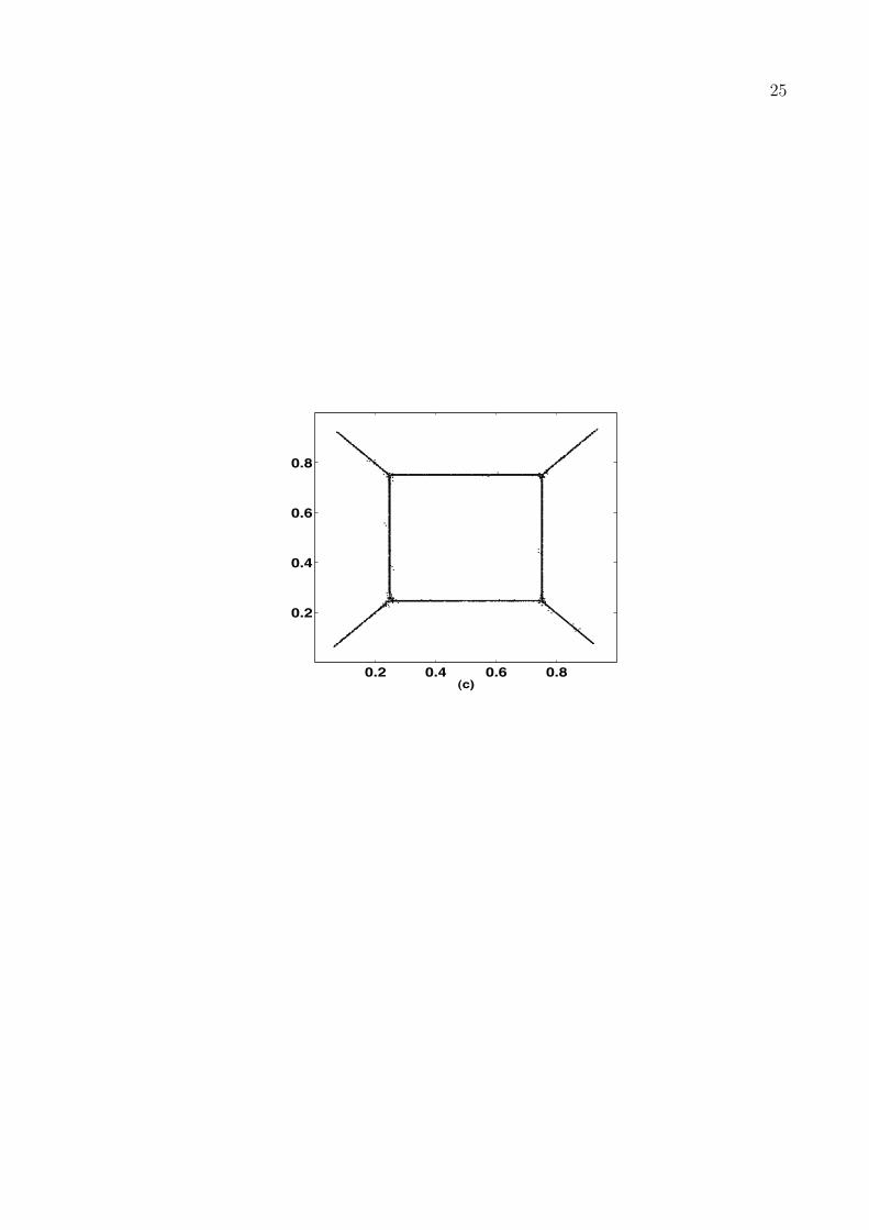
}has four knots of order three. Figure 4(a) shows a typical realisation of noisy

regression surface data, where increasing brightness corresponds to a larger surface

value. For the kernel K, we used the function K(x(1), x(2)) = (3/π) {1 − (x(1))2 −(x(2))2}2 for ‖x‖ ≤ 1 and vanishing elsewhere.

Place Figure 4 here, please

Bandwidths were selected in the interval [0.01, 0.08], using the automated

method discussed in subsection 3.2. The thresholds t1 and t2 would typically depend

on the bandwidth h, and could hence vary as well. In the present example, how-

ever, simply choosing the thresholds as constants yielded good results, as illustrated

in Figure 4(b). We took δ = 0.3 and t2 = 0.03, and chose t1 very small; almost

identical results were obtained for values of t1 within a wide range. Figure 4(c)

shows the aggregated result over 20 realisations, which is essentially a histogram

11

over 400× 400 bins with vertices coinciding with those of a regular grid on the unit

square. For easier visual interpretation, we set all non-zero values of histogram bins

equal to a single value, represented by black dots in Figure 4(c).

We performed cyclic location re-fitting, which meant that we shifted the current

estimate at the edge by a small amount along the normal to the estimated tangent

direction. This idea was used by Hall & Rau (2000). Tracking of an edge was

terminated if the estimate came within 0.08 of the boundary of the unit square.

The initial point x0 was located by searching in the left half of the unit square with

the constraint x(2) = 0.5.

3.2. Application to real image

In the computer vision literature, the ‘Cameraman’ image has been used extensively

as a benchmark. We employed a greyscale, 256 × 256 pixel version of this image.

The image domain was the unit square [0, 1] × [0, 1], and we restricted ourselves

to estimating the edge graph within the sub-window Π = [0.25, 0.75]× [0.37, 0.87].

Figure 5 depicts the original image restricted to Π.

Place Figure 5 here, please

Panels (a) and (b) of Figure 3.3 depict the two estimates of the boundary

obtained by applying the Sobel and the Laplacian of Gaussian (LoG) methods,

respectively. See Qiu (2005, section 6.2) for discussion of LoG. For both panels (a)

and (b), thresholds were chosen to give the best visual impression. The parameters

used in Figure 6(a) and (b) were selected for the original image, where 256 potential

grey levels were coded as the integers 0, 2, . . . , 255. Pixel intensities were divided

by 256, so as to yield a regression function with values in [0, 1).

Place Figure 6 here, please

As was to be expected from the visual impression, a simulation using a single

starting point did not suffice to estimate more than a part of the edge graph. To

maximise coverage, we therefore started the algorithm at several points determined

as change points in a line search, resulting in starting points x0 = x0,r =(x

(1)0,r, x

(2)0,r

).

Here x(2)0,r = 0.38+0.015 r, and x(1)

0,r was estimated within the interval (ar, br) where

a3m = a0 = 0, a3m+1 = a1 = 1/3, a3m+2 = a2 = 2/3 (m ≥ 1), and br = ar + 1/3,

r = 0, . . . , 29. If the added edge graph component was too short (which we took

as less than five points) or there was no edge detected at all, no points were added

to the graph estimate. Tracking was stopped as soon as the estimate reached the

12

boundary of Π. Since data outside Π were retained, no boundary effects needed to

be taken into account.

We took the thresholds t1 and t2 to vary in proportion to h5/2, with h denoting

the bandwidth. We estimated h locally, as follows. For a given bandwidth and at

a given point, we estimated derivatives as regression coefficients in a piecewise-

linear approximation on each of four square-shaped quarter-neighbourhoods of that

point. These neighbourhoods are defined as in Qiu (2004) in the context of surface

estimation, but were rotated by the estimated slope (called θ at (5)) from the

previous step. The Euclidean norm of the gradient in the two subsquares with the

smallest residual sum of squares from the previous surface fitting step, was then

minimised as a function of h. This gave bandwidths in the interval [0.01, 0.03].

To lessen the variation, bandwidths were calculated as moving averages, with the

currently computed bandwidth and the two previous ones being given weights 0.6,

0.3 and 0.1, respectively. We took δ = 0.3, and did not stop tracking until the

algorithm got as close as 0.006 to a previously tracked point. The rule for taking a

point to be a corner was that in subsection 3.1.

Figure 6(c) shows the obtained estimate as the raw points, which numbered 734

in total, and panel (d) shows the estimate obtained by linearly connecting the points

in (c), alongside the detected corners and knots. The salient features of the images

appear more clearly outlined than for the Sobel and LoG methods, with detected

edges being both thin and well connected. Also, the front part of the camera, which

has a very diffuse mixture of grey levels, is rendered surprisingly well, except for the

fact that the top lens is missing. Performance on other real-world images of similar

overall complexity also yielded good results, with generally only few parameters

besides t1, t2 requiring adjustment.

An important issue is to assess the quality of estimation. This may be done

visually, as is commonly done in practice, but this is well known to be in discordance

with performance in various Lp metrics. In principle, a suitable metric should take

the number of false positives and negatives of knots and corners into account; if there

is a simple procedure for this then we have not found it. If one assumed a ground

truth of edges in this or another image, we think that one of the distances suggested

in Qiu (2002; 2005, section 4.4) would be suitable, with the caveats mentioned there.

13

4. Theory

4.1. Main results

We suppose that the response surface is given by the equation y = f(x), where f is

a function from IR2 to IR. Data pairs (Xi, Yi) are observed, generated by the model

Yi = f(Xi)+ei, where the Xi’s are points in the plane IR2. Conditional on the set Xof all Xi’s, the errors ei are assumed to be independent and identically distributed

random variables with zero mean and a distribution which does not depend on Xand has finite moment generating function in a neighbourhood of the origin. Further

regularity conditions, (a)–(g), are given in Appendix 1. In particular, (a) implies

that the points Xi are distributed with density approximately equal to ν per unit

area of IR2.

Under these assumptions we generate a sequence of datasets Z = {(Xi, Yi),

−∞ < i < ∞}, indexed by the positive real parameter ν which, for simplicity, we

take to be integer valued and which will be allowed to diverge to infinity. As ν

increases, the points Xi become increasingly dense in IR2. The assumptions require

us to interpret G as a particular set of curves in the Cartesian plane, and so confer

on G a metric rather than a merely topological character.

Recall that the estimator G of G was defined in subsection 2.5 by a five-part

tracking algorithm. Suppose G has exactly mk vertices of degree k for 1 ≤ k ≤ k0.

Part (i) of the theorem below states that, with probability converging to 1 as the

density of design points increases, the tracking algorithm correctly identifies the

numbers of vertices of each degree, and in particular does not add any extra vertices.

Part (ii) declares that vertices of degrees 2 or more are estimated to within O(ε),

where ε = (νh)−1 log ν + h2, of their true locations. This degree of accuracy is not

necessarily achieved for vertices of degree 1, although part (iii) shows that vertices

of degree 1 are estimated consistently. Part (iv) states that edges of G are estimated

with accuracy O(ε), and part (v) shows that the tangents of edges of G are estimated

with accuracy O(ε/h).

Let D0, D1 and D2 denote, respectively, the distance of an identified vertex

from the nearest actual vertex of G, the supremum of D0 over all identified vertices

of degree 1, and the supremum of D0 over all identified vertices of degree at least 2.

Given x ∈ G, let D(x) equal the distance of x to the nearest point of G, and

write G(x) for the absolute value of the difference between the estimated gradient

14

of G at x, and the actual gradient of G at the point of G nearest to x. Define

Dsup = supx∈G D(x) and Gsup = sup

x∈G G(x). An outline proof of the following

theorem is given in Appendix 2.

Theorem. Assume conditions (a)–(g). Then with probability 1, (i) for all suffi-

ciently large ν the algorithm identifies exactlymk vertices of degree k for 1 ≤ k ≤ k0;

(ii) D2 = O{(νh)−1 log ν + h2}; (iii) D1 = o(1); (iv) Dsup = O{(νh)−1 log ν + h2};and (v) Gsup = O{(νh2)−1 log ν + h}.

Choosing h to be of size α = (ν−1 log ν)1/3, for example to equal Cα for some

C > 0, we deduce from the theorem that in the Poisson case, all the errors in

estimating points on G, be they vertices or points on smooth edges, equal O(α2).

This is within the factor (log ν)2/3 of the minimax-optimal pointwise rate, ν−2/3,

for estimating a smooth edge that has bounded curvature. Likewise, we see from

the theorem that for Poisson-distributed data, the convergence rate of our slope

estimator, at smooth parts of edges, is O{ν−1/3(log ν)2/3}. For gridded data, taking

h = Cβ, where β = (ν−1 log ν)1/4, we see from the theorem that the convergence

rate of our estimator, at smooth parts of edges, is O(β1/4), which again is within a

logarithmic factor of the minimax-optimal pointwise rate.

5. Discussion

In this final section, we summarise some observations on the application of the

algorithm (subsection 2.5) which emerged from our experiments with real-world

images, and which we hope to be helpful in practice. We first comment on aspects

of the algorithm, in the order described in subsection 2.5, and conclude with some

remarks of a general nature.

Regarding step (1): Among the recommendations that we make, one of the

easiest is with regard to the choice of the starting point; see subsection 2.6. We

recommend the use of many line transects rather than a single one. These may

be chosen deterministically or even at random; as the example in subsection 3.2

illustrates, this enables capturing as large a portion of G as possible. Note that

each of these starting points will have a relatively large value of T0 (defined at (4)),

and it is therefore plausible to select the threshold t1 as a fraction of this initial

value.

Regarding step (2): We suggest that it is a good idea to use a rather small

15

value of δ, not much larger than δ = 0.1 which was used in section 3. Also, it may

be expedient (though this is arguable) not to allow any knots to be detected if one

had been detected within the last q (say) steps. We took q = 5.

Regarding step (3): In our simulations in subsection 3.2, we detected rather

many knots, which were the result of small-scale image intensity variation and

ensuing small edge segments. In order to be more sure of detecting ‘genuine’ knots,

one may increase t2 but in this way, many ‘genuine’ knots are not detected either.

In images somewhat ‘simpler’ than this, with a well connected edge graph, this may

not be too problematic if the (visually anticipated) knot is reached from another

direction (if the edge graph is sufficiently connected or many starting points are

used, as suggested above). Such a point may then be declared a knot even if this

had not been done when the algorithm first passed that point.

In the detection of knots as well as corners, it is necessary to specify the mini-

mum angle of the ray(s) that separates emanating from the point in question. Note

that this may be seen as the finite-sample analogue of the “sharp vertex” assump-

tion from the first paragraph of subsection 2.1. We found that using a value below

40◦, we would get spurious corners on the top of the head and shoulders of the

cameraman, which arise to due small-scale undulations. For similar reasons, we

found it efficacious to restrict angles between rays at knots of order three to values

no less than 45◦.

Regarding step (4): We found that the line segment L(xj−1, θ) is generally

too long to give good performance. Specifically, the first new point on a ray at

a knot is placed too far away from the knot and hence the emanating new edge

may be missed altogether. Shortening that segment to half of its length is, as our

experiments suggest, advantageous in practice.

Regarding step (5): We note that the matter of linking up edge pieces is far

from straightforward. As a case in point, the presence of small features with high

curvature parts such as the ear of the cameraman may make it advisable to link

edges only when they are much closer than (1 + δ)h. Of course, when checking

for the nearest neighbours in the edge hitherto tracked, one always has to exclude

several immediately preceding points.

We conclude with general comments. The potential of automation already

emerges from the discussion above, but the most intricate problem in this regard

16

concerns the choice of bandwidth, and we see a lot of scope and necessity for future

work here. Assumption (g) in Appendix 1 prescribes that tj = o(νh2) for j = 1

and 2, and the choice tj ∼ h5/2 from subsection 3.2 seems to work well in practice.

On the question of how to determine the implied constants in those thresholds, in

the case of t1, the method described above may be a satisfactory answer. As to the

choice of t2, we recommend to check — possibly within a smaller sub-window only

— for the number of knots detected with a relatively large threshold, and gradually

decreasing the multiplier and hence t2 until the number of knots roughly matches

the possible expectation (if only a rough one) of the observer. To us, at least a

partial automation of this procedure seems possible.

Acknowledgement. We are grateful to two reviewers for helpful comments.

References

Achour, K., Zenati, N. & Laga, H. (2001). Contribution to image and contourrestoration. Real-Time Imaging 7, 315–326.

Bhandarkar, S.M. & Zeng, X. (1999). Evolutionary approaches to figure-groundseparation. Appl. Intell. 11, 187–212.

Bhandarkar, S.M., Zhang, Y.Q. & Potter, W.D. (1994). An edge-detection techniqueusing genetic algorithm-based optimization. Patt. Recognition 27, 1159–1180.

Chan, F.H.Y., Lam, F.K., Poon, P.W.F., Zhu, H. & Chan, K.H. (1996). Objectboundary location by region and contour deformation. IEEE Proc. Vis.

Image Sig. Process. 143, 353–360.

Eubank, R.L. & Speckman, P.L. (1994). Nonparametric estimation of functionswith jump discontinuities. In: Change-point problems, Eds. E. Carlstein,H.-G. Muller & D. Siegmund, IMS Lecture Notes 23, pp. 130–144. Instituteof Mathematical Statistics, Hayward, CA.

Forsyth, D. & Ponce, J. (2003). Computer vision: a modern approach, 2nd edn.Prentice Hall, London.

Gonzalez, R.C. & Woods, R.E. (1992). Digital image processing. Addison-Wesley,Reading, MA.

Hall, P., Peng, L. & Rau, C. (2001). Local likelihood tracking of fault lines andboundaries. J. R. Statist. Soc. Ser. B 63, 569–582.

Hall, P. & Rau, C. (2000). Tracking a smooth fault line in a response surface. Ann.

Statist. 28, 713–733.

Haralick, R.M. & Shapiro, L.G. (1992). Computer and robot vision, vol. 1 Addison-Wesley, Reading, MA.

17

Hartley, R. & Zisserman, A. (2001). Multiple view geometry in computer vision.Cambridge University Press, Cambridge, UK.

Jahne, B. & Haussecker, H. (2000). Computer vision and applications: a guide for

students and practitioners. Academic Press, San Diego.

Kang, D.J. & Kweon, I.S. (2001). An edge-based algorithm for discontinuity adap-tive color image smoothing. Patt. Recog. 34, 333–342.

Kang, D.J. & Roh, K.S. (2001). A discontinuity adaptive Markov model for colorimage smoothing. Image Vis. Comput. 19, 369–379.

Li, S.Z. (1995a). Markov random field modeling in computer vision. Springer, Tokyo.

Li, S.Z. (1995b). On discontinuity-adaptive smoothness priors in computer vision.IEEE Trans. Patt. Anal. Mach. Intell. 7, 576–586.

Li, S.Z. (2000). Roof-edge preserving image smoothing based on MRFs. IEEE Trans.

Image Process. 9, 1134–1138.

Miyajima, K. & Mukawa, N. (1998). Surface reconstruction by smoothness mapestimation. Patt. Recog. 31, 1969–1980.

Mallat, S.G. (1999). A wavelet tour of signal processing, 2nd edn. Academic Press,San Diego.

Morel, J.-M. & Solimini, S. (1995). Variational methods in image segmentation.Birkhauser, Boston.

Muller, H.-G. (1992). Change-points in nonparametric regression analysis. Ann.

Statist. 20, 737–761.

Muller, H.-G. & Song, K.S. (1994). Maximin estimation of multidimensional bound-aries. J. Multivar. Anal. 50, 265–281.

O’Sullivan, F. & Qian, M.J. (1994). A regularized contrast statistic for object bound-ary estimation — implementation and statistical evaluation. IEEE Trans.

Patt. Anal. Mach. Intell. 16, 561–570.

Park, S.C. & Kang, M.G. (2001). Noise-adaptive edge-preserving image restorationalgorithm. Opt. Eng. 39, 3124–3137.

Parker, J.R. (1997). Algorithms for image processing and computer vision. Wiley,New York.

Pedersini, F., Sarti, A. & Tubaro, S. (2000). Visible surface reconstruction withaccurate localization of object boundaries. IEEE Trans. Circ. Syst. Video

Tech. 10, 278–292.

Qiu, P.H. (1998). Discontinuous regression surfaces fitting. Ann. Statist. 26, 2218–2245.

Qiu, P.H. (2002). A nonparametric procedure to detect jumps in regression surfaces.J. Comput. Graph. Statist. 11, 799–822.

Qiu, P.H. (2004). The local piecewisely linear kernel smoothing procedure for fittingjump regression surfaces. Technometrics 46 (1), 87–98.

18

Qiu, P.H. (2005). Image processing and jump regression analysis. Wiley, New York.

Qiu, P.H. & Yandell, B. (1997). Jump detection in regression surfaces. J. Comput.

Graph. Statist. 6, 332–354.

Qiu, P.H. & Yandell, B. (1998). A local polynomial jump-detection algorithm innonparametric regression. Technometrics 40, 141–152.

Sinha, S.S. & Schunck, B.G. (1992). A 2-stage algorithm for discontinuity-preservingsurface reconstruction. IEEE Trans. Patt. Anal. Mach. Intell. 14, 36–55.

Yi, J.H. & Chelberg, D.M. (1995). Discontinuity-preserving and viewpoint invariantreconstruction of visible surfaces using a first-degree regularization. IEEE

Trans. Patt. Anal. Mach. Intell. 17, 624–629.

C. Rau, Department of Mathematics, Hong Kong Baptist University, Kowloon Tong,Hong Kong.E-mail: rau@math.hkbu.edu.hk

Appendix 1: Regularity conditions for theorem

(a) The Xi’s are either arranged deterministically on a regular triangular, squareor hexagonal grid with density ν per unit area of IR2, or are the points of a Poissonprocess with intensity νψ in the plane. The function ψ, not depending on ν, isassumed bounded away from zero on an open set S ⊆ IR2, and is taken to beidentically equal to 1 when the points Xi are arranged on a grid. If the points Xi

are all located at vertices of a regular grid then it is assumed the grid is supportedthroughout IR2.

(b) The planar graph G ⊆ S is connected and contains only finite numbers of edgesand vertices; each edge between two vertices has a continuously turning tangentand bounded curvature; the degree of each vertex does not exceed a given integerk0 ≥ 1; and, for each k ≥ 3, any point x of G which can be written as the limit alongexactly k nondegenerate edge segments of G, all of the segments distinct except thateach contains x, is a vertex of degree k. If exactly two of these smooth edges meetat a point where the angle between their tangents does not equal 0 or π, then thatpoint is a vertex of degree k = 2.

(c) The function f is continuous and has a uniformly bounded derivative in S \ G.For each x ∈ G, f(y) has a well-defined limit as y → x through any line segmentL(x) that has one end at x and, excepting this point, is entirely contained in S \ G.

(d) For each x ∈ G, write L1(x) and L2(x) for two versions of L(x), as introducedin (c) but having the following additional properties: given a small number η1 > 0,let vr ∈ Lr be distant exactly η1 from xj ; and suppose that for all sufficiently smallη1 the line that joins v1 and v2 does not lie entirely in S \G. Let d{L1(x),L2(x)} =|u1−u2|, where ur denotes the limit of f(y) as y → x through points on Lr(x), andwrite d(x) for the infimum of d{L1(x),L2(x)} over all choices of L1(x) and L2(x)

19

that satisfy the conditions in the previous sentence. We assume that for each η2 > 0,d(x) is bounded away from zero uniformly in all points x ∈ G that are distant atleast η2 from each vertex of degree 1.

(e) The bandwidth h = h(ν) satisfies h → 0 and ν1−ηh2 → ∞, for some η > 0,as ν → ∞. The kernel K is a nonnegative, radially symmetric probability density,Holder continuous in the plane and with its support equal to the unit disc centredat the origin. Moreover, the constant δ, used to define the step length δh, lies in theinterval (0, 1).

(f) For some point y ∈ G which is not a vertex, for some constant C > 0, and ateach stage ν of the sequence of datasets Z, the initial point x0 is within Ch2 of y.

(g) (Recall that t1 and t2 are the two thresholds.) For some c > 0, and for j = 1and 2, νc = O(tj) and tj = o(νh2).

Appendix 2: Outline proof of theorem

A.1. Outline proof of theorem. To appreciate why it is possible to assert, in thetheorem, that an event occurs “with probability 1” as ν → ∞, rather than merely“with probability converging to 1”, we note that it is necessary only to show thatthe probability of the event, for given ν, equals 1 − O(ν−2) as ν → ∞. (This isreadily done using the exponential bounds employed by Hall et al. (2001).) Then itwill follow from the discreteness of ν, via the Borel-Cantelli lemma, that the desiredassertion indeed holds true with probability 1.

We shall show that, if the algorithm starts at a point x0 that satisfies condition(f); and if the initial step is in the direction towards a vertex of degree k1 ≥ 2;then with probability 1, for all sufficiently large ν, the algorithm correctly deducesthe degree of the vertex [call this result (R1)], and with probability 1, for all suf-ficiently large ν, gets its location right to within O(ε) [result (R2), say], whereε = (νh)−1 log ν+h2. We shall also prove that if the vertex towards which we moveat the first step is of degree 1, then with probability 1, for all sufficiently large ν, thealgorithm gets the degree of this vertex correct [result (R3)], and gets its positionright to within o(1) [result (R4)]. Moreover, at those points of the trajectory beforewe determine that we are close to a vertex, the location and the slope of the edgeestimator are accurate to within O(ε) and O(ε/h), respectively [result (R5)].

These results can be developed into a complete proof of the theorem. Thisis done by considering restarting the algorithm (as prescribed in subsection 2.5)at the vertex estimator, moving away from that vertex along each edge estimator;using methods identical to those below to prove the analogous properties over thesubsequent edges of the graph; and noting that with probability 1, for all sufficientlylarge ν only a finite number of such stages is involved. If this is done, then properties(i)–(v) in the theorem follow from, respectively, results (R1) & (R3), (R2), (R4), (R5)and (R5).

Observe that we may write

Tk(x0) = 2∑

i

{Yi − 1

2 (fki + fk+1,i)}

(fk+1,i − fki)Ki , (6)

20

where fki = fk(Xi |x0, θ1, . . . , θk, c1, . . . , ck), with an analogous formula applyingfor fk+1,i, and, here and below, we write simply Ki for Ki(x0). Put

Ikji ={

1 if fk(Xi |x0, θ1, . . . , θk, c1, . . . , ck) = cj0 otherwise ,

and note that∑

i (Yi − cj)Ki Ikji = 0. It follows that∑

i Yi fkiKi =∑

i f2kiKi,

with the analogous result holding if k is replaced by k + 1. Therefore, by (6),

Tk(x0) =∑

i

(f2

k+1,i − f2ki

)Ki . (7)

Now, f0i does not depend on i, from which property, and (7) in the casek = 0, it follows that T0(x0) =

∑i (f1i − f0i)2Ki. A similar argument shows that

if we define c1θ and c2θ to be the quantities c1 and c2 that minimise∑

i {Yi −f1(Xi |x0, θ, c1, c2)}2Ki, for fixed θ, and put f1i(θ) = f1(Xi |x0, θ, c1θ, c2θ), thenthe following is a definition alternative, but equivalent, to that at (4):

T0(x0) = supθt(θ) where t(θ) = t(x0, θ) =

∑i

{f1i(θ)− f0i

}2Ki . (8)

Using the representation (8), and employing the argument in the appendix ofHall et al. (2001), the following can be proved. If we start the algorithm at a pointx0 which satisfies assumption (f) then, with probability 1, the subsequent pointsgenerated by the algorithm, up until the point immediately preceding the one (xj ,say; the same xj as in step (3) of the algorithm in subsection 2.5) at which weconclude we are close to a vertex, are uniformly within O(ε) of the nearest pointson G, and the gradient estimates are uniformly within O(ε/h) of the gradients atthe respective nearest points. This gives result (R5).

Let c denote the constant appearing in condition (g), imposed on the thresholdst1 and t2. If the vertex towards which the first of the above sequence of steps is takingus is of degree 1 then the following can be proved to hold. (I) With probability 1, forall sufficiently large ν, one of the sequence of values T0(x`), for ` ≥ 1, will fall belowνc strictly before one of the sequence of values of max2≤k≤k0 Tk(x`) exceeds t2.(II) If ∆ denotes the distance from the vertex (of degree 1) at which T0(x`) firstdrops below νc, then ∆ → 0 with probability 1. Properties (I) and (II) imply thatwith probability 1, for all sufficiently large ν the algorithm correctly identifies thedegree of the vertex of degree 1 [result (R3)]; and moreover, the distance betweenthe point at which the algorithm stops, and the vertex of degree 1, converges to 0[result (R4)].

Assume next that the first in the sequence of steps discussed two paragraphsabove takes us in the direction of a vertex, z say, of degree k1 ≥ 2. Recall thatδh equals step length. It can be proved that with probability 1, for all sufficientlylarge ν the point xj−1 at which the sequence terminates is within (1 + δ)h of z. Letζ = ζ(ν) denote any positive sequence of constants decreasing to 0 as ν → ∞, so

21

slowly that ζν1−ch2 →∞, where c is the constant in condition (g) on the thresholdvalues. Recall the definition of L(xj−1, θ) given in step (3) of the algorithm, insubsection 2.5. Since the vertex at z is of degree k1 ≥ 2 then we may prove from (A.2)that with probability 1, the following are true: (III) for all η > 0, sup inf Tk(x) =O(νη), where the supremum is over all k ∈ [k1, k0] and the infimum is over allx ∈ L(xj−1, θ); and (IV) for all sufficiently large ν, ζνh2 ≤ inf Tk(x), where nowthe infimum is over all k ∈ [0, k1 − 1] and all x ∈ L(xj−1, θ).

Hence, noting the definition of k in step (3) of the algorithm, and the conditionson t2 imposed in assumption (g), we deduce that with probability 1, k = k1 for allsufficiently large ν. This gives result (R1). Noting that with probability 1, (V) xj−1

is distant O(ε) from the nearest point on G, (VI) the slope estimator θ at xj−1 is inerror by only O(ε/h), and (VII) for all sufficiently large ν, z is itself within (1+ δ)hfrom xj−1, we conclude that: with probability 1, the point z is perpendicularlydistant O(h2) from the line segment along which we search for our estimator of z.This fact, and property (7), may be used to establish result (R2).

Caption for Figure 1: Planar graph, G. Vertices A, B, C and D in the graph areof degrees 1, 2, 3 and 4, respectively. In particular, vertex A is the endpoint of anedge.

Caption for Figure 2: Perspective depiction of the surface represented by y =f(x), for x ∈ IR2. This f satisfies condition (F) for a graph G simpler than the oneshown in Figure 1.

Caption for Figure 3: Perspective representation of surface defined by y = f1(x),for x ∈ IR2, with f1 given by (2).

Caption for Figure 4: Panel (a) shows the noisy response surface defined by thefunction f from section 3, where the error distribution is N(0, σ2) with σ = 0.25.Panel (b) shows a realisation of the tracking estimate G, corresponding to (a). Theestimate was computed as described in subsection 2.5. The four estimated knotsare circled. Panel (c) shows the result of aggregating 20 realisations as described insection 3.

Caption for Figure 5: Central part of original Cameraman image, as used forestimation.

Caption for Figure 6: Panels (a)–(c) show estimates of the edge obtained by theSobel, Laplacian of Gaussian (LoG), and the method of this paper, respectively.The circled points in panel (c) are the knots of order three. Panel (d) shows theresults after linearly connecting the sequence of points from (c), alongside the knotsand corners. In each of panels (a)–(d) a small rim around the estimation window Πis added for visual purposes.

22

A

D

C

B

Fig. 1. Planar graph, G. Vertices A, B, C and D in the graph are of degrees 1, 2, 3and 4, respectively. In particular, vertex A is the endpoint of an edge.

23

Fig. 2. Perspective depiction of the surface represented by y = f(x), for x ∈ IR2. This fsatisfies condition (F) for a graph G simpler than the one shown in Figure 1.

!"

!

#$!!""#!$

#!!!""#!$

Fig. 3. Perspective representation of surface defined by y = f1(x), for x ∈ IR2, with f1

given by (2).

24

(a)

!

!"

"

0.2 0.4 0.6 0.8

0.2

0.4

0.6

0.8

0.2 0.4 0.6 0.8

0.2

0.4

0.6

0.8

(b)

Fig. 4. Panel (a) shows the noisy response surface defined by the function f from section 3,where the error distribution is N(0, σ2) with σ = 0.25. Panel (b) shows a realisation ofthe tracking estimate G, corresponding to (a). The estimate was computed as describedin subsection 2.5. Panel (c) shows the result of aggregating 20 realisations as describedin section 3.

25

0.2 0.4 0.6 0.8

0.2

0.4

0.6

0.8

(c)

26

x1

x2

0.4 0.6

0.4

0.6

0.8

Fig. 5. Central part of original Cameraman image, as used for estimation.

27

Sobel (threshold =20)

(a)

LoG (s=1,k=9,threshold =15)

(b)

Raw Graph Estimate

(c) (d)

Interpolating Linear Estimate

Corners

Knots of Order 3

(a)

Sobel (threshold =20)

(a)

LoG (s=1,k=9,threshold =15)

(b)

Raw Graph Estimate

(c) (d)

Interpolating Linear Estimate

Corners

Knots of Order 3

(b)

(c)

Corners

Knots of Order 3

(d)

Fig. 6. Panels (a)–(c) show estimates of the edge obtained by the Sobel, Laplacian ofGaussian (LoG), and the method of this paper, respectively. The circled points in panel(c) are the knots of order three. Panel (d) shows the results after linearly connecting thesequence of points from (c), alongside the knots and corners. In each of panels (a)–(d) asmall rim around the estimation window Π is added for visual purposes.