trabajo de fin de grado -...

Equation Chapter 1 Section 1

Trabajo de Fin de Grado

Grado en Ingeniería de Tecnologías de

Telecomunicación

Mejoras en el OCR Tesseract

Autor: Jesús Bocanegra Linares

Tutor: Rafael María Estepa Alonso

Departamento de Telemática

Escuela Técnica Superior de Ingeniería

Universidad de Sevilla

Seville, 2016

Final Major Project

Degree in Engineering of Technologies of Telecommunications

Specialty of Telematics

Improvements for Tesseract OCR

Case analysis for automatic transcription of ancient books at the

Library of the Universidad de Seville

Author:

Jesús Bocanegra Linares

Supervisor:

Rafael María Estepa Alonso

Doctor Professor

Field of knowledge: Telematic Engineering

Department of Telematics

Superior Technic School of Engineering

University of Seville

Seville, 2016

Trabajo de Fin de Grado

Grado en Ingeniería de las Tecnologías de Telecomunicación

Intensificación de Telemática

Mejoras en el OCR Tesseract

Estudio de caso para la transcripción automática de libros

antiguos en la Biblioteca de la Universidad de Sevilla

Autor:

Jesús Bocanegra Linares

Tutor:

Rafael María Estepa Alonso

Doctor Profesor

Área de Conocimiento: Ingeniería Telemática

Departamento de Telemática

Escuela Técnica Superior de Ingeniería

Universidad de Sevilla

Sevilla, 2016

Trabajo de Fin de Grado: Mejoras en el OCR Tesseract

Autor: Jesús Bocanegra Linares

Tutor: Rafael María Estepa Alonso

El tribunal nombrado para juzgar el Proyecto arriba indicado, compuesto por los siguientes miembros:

Presidente:

Vocales:

Secretario:

Acuerdan otorgarle la calificación de:

Sevilla, 2016

El Secretario del Tribunal

To my family

To my teachers

Acknowledgments

I would like to express my appreciation to my supervisor Rafael Estepa for his useful comments

and support. Moreover, I would like to thank Brynn Chivers, CS student at Pacific University,

Oregon, for her proofreading of the text. Furthermore, I would like to show my gratitude to the

Library of the University of Seville for their confidence and the use of server infrastructure.

Finally, I am also grateful to my family for their support and backup along the whole major.

Abstract

The Library of the University of Seville owns a rich collection of antique works that are being

scanned. In order to make the access to information easier, they need the full text of these books.

An automated transcription solution is sought since the task is too time-consuming for humans. To

achieve this, different existing solutions are analyzed, such as veteran open source programs and

cutting-edge neural networks technologies. After the research, a concrete solution is provided to

the Library, along with guidelines for its execution.

Index

Acknowledgments 13

Abstract 15

Index 17

Illustration Index 19

Code snippets Index 21

1 Introduction and goals 23 1.1 Motivation 23 1.2 Special difficulties with antique books 23 1.3 Purpose of this project 24

2 State of the art 25 2.1 Brief overview of common OCR solutions 25

2.1.1 Proprietary software 25 2.1.2 Free solutions 25

2.2 Tesseract OCR 25 2.2.1 Overall operation of the recognition algorithm 26

2.3 Artificial Neural Networks 27 2.3.1 Artificial Neurons 27 2.3.2 Transfer functions 28 2.3.3 Layers 30 2.3.4 Softmax function 30 2.3.5 Training 31 2.3.6 Testing 31 2.3.7 Kinds of Neural Networks 31 2.3.8 Universality 32

2.4 Libraries for Artificial Neural Networks 32 2.5 TensorFlow 33

2.5.1 TensorBoard 33 2.6 Academic proposals 35

2.6.1 Specific algorithm: feature extraction 35 2.6.2 All-purpose Artificial Intelligence algorithm: Artificial Neural Networks 35 2.6.3 Chosen option 36

3 Proposed solution 37 3.1 Details of the proposed solution 37 3.2 Distributed architecture proposal 39

3.2.1 Master server 39 3.2.2 Slave 40

4 First draft and results 43 4.1 Structure of the neural network 43 4.2 Structure of the program 44

4.3 Results of the first-approach solution 45 4.3.1 Training preparation 45 4.3.2 Training 46 4.3.3 Classifier 47

5 Conclusion 49 5.1 Future guidelines 49 5.2 Challenges 49

6 Annex: training Tesseract 51 6.1 Compiling Tesseract 51 6.2 Setup and use 52 6.3 Training 53

7 Annex: Code of the initial OCR 55 7.1 Training data preparation 55 7.2 Training code 59 7.3 Character classification 61

8 Annex: Project planning 64 8.1 Project cost 64

8.1.1 Cost details 64 8.2 Time planning 65

9 Summary in Spanish / resumen en español 71 9.1 Introducción y objetivos 71

9.1.1 Motivación 71 9.1.2 Dificultades especiales con libros antiguos 71 9.1.3 Propósito del proyecto 72

9.2 Estado del arte 72 9.2.1 Visión de conjunto de OCR existentes 72 9.2.2 Tesseract OCR 73 9.2.3 Redes Neuronales Artificiales 73 9.2.4 Bibliotecas para Redes Neuronales Artificiales 75 9.2.5 TensorFlow 76 9.2.6 Propuestas académicas 76

9.3 Solución propuesta 77 9.3.1 Detalles de la solución propuesta 77 9.3.2 Propuesta de arquitectura distribuida 78

9.4 Primer borrador y resultados 80 9.4.1 Estructura de la red neuronal 80 9.4.2 Resultados 80

9.5 Conclusiones 81 9.5.1 Futuras líneas de avance 81 9.5.2 Desafíos 81

References 83

ILLUSTRATION INDEX

Illustration 1: Artificial Neuron ......................................................................................................... 27

Illustration 2 : Logistic function ........................................................................................................ 28

Illustration 3: Logistic function’s derivative .................................................................................... 29

Illustration 4: Rectifier function ........................................................................................................ 29

Illustration 5: Derivative of rectifier function................................................................................... 30

Illustration 6: Neural network with hidden two layers. From [3] by Michael Nielsen, under CC

BY-NC 3.0 license. ............................................................................................................................ 30

Illustration 7: Typical architecture for a CNN. By “Aphex34” and licensed under CC BY-SA 4.0

............................................................................................................................................................. 32

Illustration 8: TensorBoard graphs section ....................................................................................... 34

Illustration 9: Events graphs in TensorFlow..................................................................................... 35

Illustration 10: Elements detected by sliding window ..................................................................... 38

Illustration 11: Summary Gantt Chart............................................................................................... 39

Illustration 12: Flow of information in solution structure ............................................................... 41

Illustration 13: Stages of the proposal development ........................................................................ 42

Illustration 14: Layer architecture ..................................................................................................... 44

Illustration 15: Structure of the draft program .................................................................................. 44

Illustration 16: Training iteration ...................................................................................................... 45

Illustration 17: Output file after training preparation ....................................................................... 46

Illustration 18: Serialized output file of the training program ......................................................... 47

Illustration 19: Estructura de una neurona ........................................................................................ 73

Illustration 20: Red neuronal con dos capas ocultas. Por Michael Nielsen, bajo licencia CC BY-

NC 3.0. ................................................................................................................................................ 75

Illustration 21: Pasos en el desarrollo ............................................................................................... 79

Illustration 22: Estructura de la red neuronal propuesta .................................................................. 80

CODE SNIPPETS INDEX

Code 1: Detail of layer setup ............................................................................................................. 43

Code 2: Results of the execution of preparation script .................................................................... 46

Code 3: Output of the training program ............................................................................................ 47

Code 4: Example classifier execution ("With probability 99.9578% the letter is a: \ G") ............ 47

Code 5: Shell-script for automated installation of Tesseract ........................................................... 52

Code 6: Training data preparation ..................................................................................................... 58

Code 7: Training ................................................................................................................................. 61

Code 8: Classifier ............................................................................................................................... 63

23

1 INTRODUCTION AND GOALS

CR (Optical Character Reconnaissance) tools have been developed since the decade of

1980 to face the challenge of automatically transcribing written text. This process consists

in acquiring a digital text representation from a physical text stored in a digital graphical

source, such as scanned images or photographs.

The advantages of having digital transcriptions of written media are numerous and well

known: preservation of the information, availability of data, ease of translation, automated search

and analysis– among others.

1.1 Motivation

The Fondo Antiguo (Ancient Collection Section) in the Library of the University of Seville has

over 100,406 ancient works of incalculable value, of which 332 are incunabula and 9,941 from the

XVI century [1]. Every day several of these works are scanned at the library workshop and an

estimated of 9,500 of them have already been digitalized.

These image files and book metadata are released into a website, so that the wealth of

knowledge they contain is available to the general public.

Having transcriptions for these texts would allow interesting options for researchers and other

public: lexical analysis; content indexation, which allows quick searching; and historical studies,

like weather or demographic investigations.

The indexation of document texts into a database is especially noteworthy, since it would allow

the information in these ancient works to be easily found on the Internet. Any user with an Internet

connection would be able to access the information even if they are not historians nor have

knowledge of paleography. This means an actual democratization of that information guarded by

the Library.

While human-made transcriptions are better quality than automatic ones, the volume of works

available and slow speed of the process make it an impossible task. Computer-driven processing

may deliver results with inaccuracies, but could still be useful for the goals enumerated above,

depending of course, on the error quantity. Using artificial intelligence algorithms is also an option

to consider in the process of minimizing these mistakes.

1.2 Special difficulties with antique books

Current OCR algorithms handle modern text recognition with ease and provide a reasonable rate

of correct matches. Nevertheless, the most interesting works in the Library’s Ancient Collection

range from the XV to XVIII centuries. This implies a higher difficulty compared to prints from

XIX century until modern day.

The most common obstacles for a computer to transcribe such texts are the following:

Dependence on the quality of the physical book and its state of preservation: The most

important items are usually several centuries old and may present deteriorations on their

pages. This damages could lead to more difficult transcription processes.

Variability of graphology: Printing types are heterogeneous among books and through the

centuries. The number of different fonts used make it difficult to recognize characters. If

O

24

an algorithm learned how to understand one typography, it would probably have trouble

classifying the symbols of another one.

Heterogeneity of the language: Most of the books of interest are written in old Castilian

and are from a time before orthography was fixed. Such a changeability makes it more

challenging to use a lexicon to fix small transcription errors.

Other unique features of old prints: Other characteristics such as abbreviations and letter

bonds may also affect transcriptions in a negative way and make the development of an

algorithm and its training harder.

In order to fulfill the development of the project, it would be necessary to aboard topics from

different fields:

History of types and print.

Diplomatics: transcription rules.

Abbreviations, shortenings and special characters, all frequent in the texts from the goal

centuries.

1.3 Purpose of this project

The goal of this work is to explore different OCR solutions and help the Library of the University

of Seville achieve automatic transcription of antique books in its own infrastructure. Provided at

the end of this research are a technological solution and guidelines.

As for the requirements, any proposal supplied to the Library may only use open source or free-

to-use technologies and never require a paid license. Another condition is that the process must to

be feasible with only the Library’s resources. Nonetheless, it may also be possible to use the help

of other public institutions. For example, the CICA (Centro Informático Científico de Andalucía,

Scientific Computing Center of Andalusia) has offered a significant part of its computing cluster.

The steps that will be taken to achieve this are:

1. Bibliographic search about existing OCR solutions and other technologies that may be

useful for the project.

2. Two possibilities will be chosen from the research. Next, it will be researched how to use

them and try and get results using them on the target works.

3. After that, a solution will be proposed considering all the research. Guidelines will be

provided for the Library to accomplish its goals regarding books transcription.

4. The final step is presenting a draft or first approach of the proposed solution and its results,

as well as the conclusions.

In short, the goal of the project is to find an OCR solution for the Library and develop a

preliminary version of it. If the chosen option was to be the development of an OCR from scratch,

the scope of the results would be a program able to identify characters one by one using an example

character set. Such a program would later need to be developed to fully understand whole pages

and characters from antique books.

This development would take a considerable amount of time. A temporal planning will be

provided for this development. The expected result of the project is not, thus, a program that

processes antique text, but a technical report and the scores of a first approximation program

applied to an existing character dataset. Thereof, using the original antique types is out of the scope

of this work due to its complexity and magnitude.

By using this report, the Library may be able to study the viability and take decisions based on

the technical information herein.

25

2 STATE OF THE ART

ptical character recognition (OCR) refers, according to [2], to “the process of translating

images of handwritten, typewritten, or printed text into a format understood by machines

for the purpose of editing, indexing/searching, and a reduction in storage size”.

Many OCR softwares currently exist. These solutions use specific algorithms to pursue a

good transcription, i.e. these procedures are specifically designed for text analysis. Such methods

often extract geometrical features from the letters to classify them.

Another schema consists in using novel artificial intelligence and machine learning

techniques. These technologies like deep learning are producing state-of-the-art results at tasks

like computer vision, automatic speech recognition and natural language processing [3].

2.1 Brief overview of common OCR solutions

This lists are not intended to be exhaustive and their purpose is just illustrative. No scientific

criteria have been used to compose them.

2.1.1 Proprietary software

Adobe Acrobat: This application has an OCR built-in tool [4].

ABBYY FineReader: Recognizes 190 languages and any mix of them [5].

Asprise OCR: Developed since 1998 [6].

OmniPage: Developed at Nuance Communications, it’s been one of the first OCR

programs to work in personal computers [7]

2.1.2 Free solutions

Tesseract: Originally developed at HP and later released as open source. Now sponsored

by Google [8]. Several sources coincide on the good quality of its results [9] [10].

CuneiForm: Developed at Cognitive Technologies, was released as freeware in 2007 and

later the engine was published as open source in 2008.

GOCR: Developed since 2000 and GNU licensed [11].

Ocrad: Another GNU project based on a feature extraction method [12].

OCRopus: Project licensed as Apache 2.0 and developed at the German Research Center

for Artificial Intelligence in Kaiserslautern, Germany; led by Thomas Breuel and

sponsored by Google [13].

2.2 Tesseract OCR

Tesseract is an OCR engine developed at Hewlett-Packard (HP) from 1984 to 1994. It began as a

PhD Thesis at the University of Bristol, published in 1987 [14]. The development of this project

stopped completely in 1994. In the next year, it was presented in the Annual Test of OCR

Accuracy, where it scored competitive results against the commercial OCR solutions existing by

O

26

then [15]. The project was frozen until 2005, when HP decided to release it as open source. Google

mainly took over the project, which is now available at a GitHub repository [16]. One of the most

important features in this OCR is its learning capabilities. Following a learning process, Tesseract

is able to improve at the classification phase for a definite font.

2.2.1 Overall operation of the recognition algorithm

Tesseract makes use of a specifically designed algorithm for the detection of text. The process

involves several phases which work from the smallest to the largest.

2.2.1.1 Block detecting

The first stage for an OCR is physical page layout analysis. It consists in splitting the input image

into either text areas or blank or graphic zones. Originally, Tesseract did not have any kind of

layout analysis capabilities, since HP already had technologies developed for that purpose. The

input to Tesseract had to have been already processed, it is, to have the input page layout split into

polygons associated to those zones [17].

When the project was released as open source in 2005, this phase was missing and needed some

development. An algorithm was developed at Google for page layout analysis using tab-stop

detection [18]. This allows the OCR to process images from books, magazines, newspapers etc.

and the algorithm is now implemented in Tesseract.

2.2.1.2 Line and word finding

The next step is to detect text units: first lines and then words. Tesseract estimates the height of the

lines in each region given by the previous phase, allowing to filter out noise and non-letter

characters, whose height is usually a small percentage of the average line height [17].

Tesseract uses quadratic splines to fit the lines, what allows the OCR to handle skewed text.

This is very common in scanned books, due to bent pages at scanning time. The algorithm

establishes several parameters out of the character height in the lines, which are later used for

classifying them.

Now, words have to be detected. This task turns out to be much easier for texts with fixed-width

characters. For the other case, Tesseract uses a specific heuristic method.

2.2.1.3 Word recognition

Afterwards, the words are chopped into characters to proceed with the recognition. Tesseract has

specialized techniques for chopping joined characters [14] and associating broken characters [17].

2.2.1.4 Character classifying

Classification in Tesseract has two steps:

1. A short list is made with character classes the unknown character might actually be. The

list is made out of the best matches in a feature search.

2. The features of the character are analyzed and used to compute the similarity with learnt

prototypes.

2.2.1.5 Linguistic Analysis

Tesseract uses a lexicon to make a decision whenever a new segmentation is being considered at

the word recognition stage. This phase helps reduce the character error rate.

27

2.3 Artificial Neural Networks

Neural Networks is a programming paradigm based on brain neurons. This biological inspired

solution allows computers to learn from observational information.

A hierarchical feature extraction strategy can be used to enable a machine to understand

complex data just like a human brain does, especially with graphic data [19]. This is achieved

splitting complex problems up into simpler pieces using a multi-layer architecture, with

progressive level of complexity.

This layers are composed by artificial neurons. Each neuron does a very simple calculation,

but the total effect among all of them produces the wanted outcome.

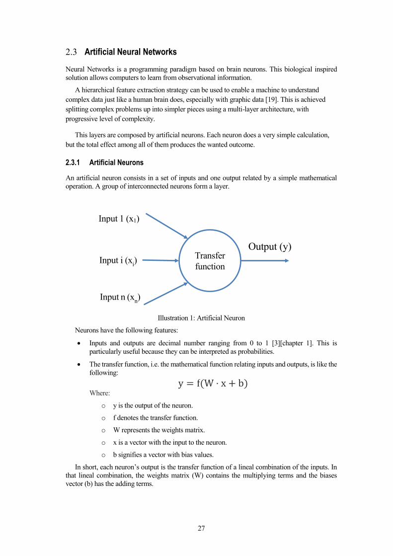
2.3.1 Artificial Neurons

An artificial neuron consists in a set of inputs and one output related by a simple mathematical

operation. A group of interconnected neurons form a layer.

Illustration 1: Artificial Neuron

Neurons have the following features:

Inputs and outputs are decimal number ranging from 0 to 1 [3][chapter 1]. This is

particularly useful because they can be interpreted as probabilities.

The transfer function, i.e. the mathematical function relating inputs and outputs, is like the

following:

y = f(W ⋅ x + b) Where:

o y is the output of the neuron.

o f denotes the transfer function.

o W represents the weights matrix.

o x is a vector with the input to the neuron.

o b signifies a vector with bias values.

In short, each neuron’s output is the transfer function of a lineal combination of the inputs. In

that lineal combination, the weights matrix (W) contains the multiplying terms and the biases

vector (b) has the adding terms.

Transfer

function

Output (y)

Input 1 (x1)

Input i (xi)

Input n (xn)

28

2.3.2 Transfer functions

There are two types of widely used transfer functions for neurons: the logistic function and the

rectifier.

2.3.2.1 Logistic function

Classified as a sigmoid function, since it is S-shaped.

σ(x) ≡1

1 + 𝑒−𝑥

Using a sigmoid function ensures that a neuron’s output can be used as other’s input

successively and guarantees numerical stability. The logistic function has a bell-shaped derivative,

which has an interesting property that makes its calculation faster.

σ′(x) =1

𝑒𝑥 (1𝑒𝑥 + 1)

2 = σ(x)(1 − σ(x))

The shape of the sigmoid functions is the key to understand why they are used for neurons. The

function has two horizontal asymptotes, limiting its values to the interval (0, 1). In addition, its S-

like shape works as a trigger, which makes it unresponsive to small inputs like noise but very

sensible to bigger inputs.

Illustration 2 : Logistic function

29

Illustration 3: Logistic function’s derivative

2.3.2.2 Rectifier function

The rectifier function is a ramp function, defined as:

𝑟(𝑥) = max(0, 𝑥)

Except at zero, its derivative is constant at each side of the origin, what is convenient for the

training process due to the speed of calculation. Using this as transfer function, the operations

needed in each neuron are just comparisons, additions and multiplications. This allow for faster

and more efficient training compared to sigmoid functions.

A neuron using this function is usually called ReLU (Rectified Linear Unit) and its efficacy has

been proven [20].

Illustration 4: Rectifier function

30

Illustration 5: Derivative of rectifier function

2.3.3 Layers

Each layer in a neural network is a set of interconnected neurons. Multilayer architectures provide

good results according to different studies like [21, pp. 11-12]. A multilayer structure identifies

with a hierarchical representation learning process. At each layer a different feature is learnt and

then recognized, leading to a hierarchy of representations with increasing abstraction level [22, pp.

17-19]. The layers connecting the input and output ones are called hidden layers.

Illustration 6: Neural network with hidden two layers. From [3] by Michael Nielsen, under CC

BY-NC 3.0 license.

2.3.4 Softmax function

Softmax layers are useful for output. They allow for classification, since they output the probability

of the input data to be every of the classes [23]. For example, a classifier recognizing 50 characters

would have a fifty neurons softmax final layer. The output of each of those neurons would be the

probability of the input image to be the class of that neuron according to the previous layers. The

output of each neuron depends on the rest of them, since their sum must be equal to 1.

The softmax function is also called normalized exponential [24, p. 198], and its expression is:

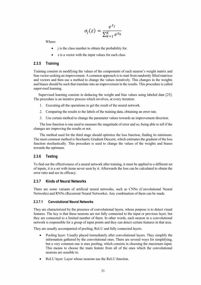
https://creativecommons.org/licenses/by-nc/3.0/deed.en_GB

https://creativecommons.org/licenses/by-nc/3.0/deed.en_GB

31

𝜎𝑗(𝑧) =𝑒𝑧𝑗

∑ 𝑒𝑧𝑘𝐾𝑘=1

Where:

j is the class number to obtain the probability for.

z is a vector with the input values for each class

2.3.5 Training

Training consists in modifying the values of the components of each neuron’s weight matrix and

bias vector seeking an improvement. A common approach is to start from randomly filled matrixes

and vectors and then use a method to change the values iteratively. This changes in the weights

and biases should be such that translate into an improvement in the results. This procedure is called

supervised learning.

Supervised learning consists in deducing the weight and bias values using labeled data [25].

The procedure is an iterative process which involves, at every iteration:

1. Executing all the operations to get the result of the neural network.

2. Comparing the results to the labels of the training data, obtaining an error rate.

3. Use certain method to change the parameter values towards an improvement direction.

The loss function is one used to measure the magnitude of error and so, being able to tell if the

changes are improving the results or not.

The method used for the third stage should optimize the loss function, finding its minimum.

The most common method is Stochastic Gradient Descent, which estimates the gradient of the loss

function stochastically. This procedure is used to change the values of the weights and biases

towards the optimum.

2.3.6 Testing

To find out the effectiveness of a neural network after training, it must be applied to a different set

of inputs, it is a set with items never seen by it. Afterwards the loss can be calculated to obtain the

error ratio and see its efficacy.

2.3.7 Kinds of Neural Networks

There are some variants of artificial neural networks, such as CNNs (Convolutional Neural

Networks) and RNNs (Recurrent Neural Networks). Any combination of them can be made.

2.3.7.1 Convolutional Neural Networks

They are characterized by the presence of convolutional layers, whose purpose is to detect visual

features. The key is that these neurons are not fully connected to the input or previous layer, but

they are connected to a limited number of them. In other words, each neuron in a convolutional

network is responsible for a group of input points and they can detect certain features in that area.

They are usually accompanied of pooling, ReLU and fully connected layers.

Pooling layer: Usually placed immediately after convolutional layers. They simplify the

information gathered by the convolutional ones. There are several ways for simplifying,

but a very common one is max pooling, which consists in choosing the maximum input.

This means to choose the main feature from all of the ones which the convolutional

neurons are sensible to.

ReLU layer: Layer whose neurons use the ReLU function.

32

Fully connected layer: Default network layer in ANN.

CNNs are effective at image recognition and natural language tasks, as published in [26].

A typical network architecture is like the following:

Illustration 7: Typical architecture for a CNN. By “Aphex34” and licensed under CC BY-SA 4.0

2.3.7.2 Recurrent Neural Networks

Neural Networks are recurrent when there are connection loops among neurons. This enables the

network to have short memory capabilities and temporal behavior.

Long Short-Term Memory [27] (LSTM) recurrent neural networks outperform classic ANN at

speech recognition, according to [28].

2.3.8 Universality

A neural network using sigmoidal functions can achieve an arbitrary good approximation of any

continuous function [3][chapter 4] by using enough hidden neurons, even in one single layer. It is:

|𝑓(𝑥) − 𝑔(𝑥)| < 𝜖

Being f the original function to estimate.

g is the output of the neural network given an input x

ϵ is the maximum approximation absolute error to achieve.

This property was mathematically demonstrated in 1989 in two different ways [29] [30].

2.4 Libraries for Artificial Neural Networks

Some of the existing libraries for Neural Networks are listed here. This list is not intended to be

exhaustive.

FANN (Fast Artificial Neural Network) Library: Open source library developed at the

Department of Computer Science at the University of Copenhagen since 2003 [31]. A

Master thesis was also published in 2007 about the algorithms used in this project [32].

It’s written in C, supports backpropagation learning and has bounds to many other

programming languages [33].

Theano: Python library capable of working both with CPUs and GPUs [34]. The Theano

Development Team is composed by researchers from many universities and corporations

[35].

OpenNN: Advanced open source library written in C++ [36].

Torch: Flexible and GPU-oriented, but uses the Lua language [37]. Developed by

scientists and engineers at Facebook, Google and Twitter.

https://creativecommons.org/licenses/by-sa/4.0/deed.en

33

Caffe: Deep learning framework developed by the Berkeley Vision and Learning Center

(BVLC) and community contributors [38].

TensorFlow: Recently (2015) [39] open-sourced (Apache 2.0 license) library by Google.

Google uses it in its services and products, such as web search.

2.5 TensorFlow

TensorFlow is an open source software library for machine learning and artificial intelligence. It

was first developed at the Google Brain Team. It can be used either with C++ or Python languages.

Some of its premier features include:

Portability: TensorFlow works on both CPUs and GPUs and on many platforms. In

addition, a program can be directly moved from research to production, almost only the

hardware changes.

Languages: It has interfaces for Python and C++, but can be extended via SWIG

(Simplified Wrapper and Interface Generator) interfaces.

Performance: The team of TensorFlow claims that the program is optimized to get the

most efficiency out of the hardware, whatever it is [40].

In TensorFlow, a calculation is defined by a set of nodes, described in Python or C++ and

usually represented graphically. This code establishes the operations to be done. Note that no actual

calculations are made until TensorFlow is told to, after these settings. [41]

The nodes have zero or more inputs and outputs and are connected to each other. These nodes

symbolize mathematical operations, and the information “flows” among them in the form of

“tensors”, thereof the name of the project. A tensor is an array of an arbitrary number of

dimensions. [41]

TensorFlow supports multi-device execution, i.e. using several devices in the same system;

and distributed execution, among different machines in the same network using mechanisms such

as TCP or RDMA (Remote Direct Memory Access).

2.5.1 TensorBoard

TensorBoard is a Python GUI tool which allows the developer to visualize the calculation flow.

Using TensorBoard in a program requires some extra coding. [Illustration 8: TensorBoard graphs

section] shows the graph for an example program, which displays the structure of the calculations.

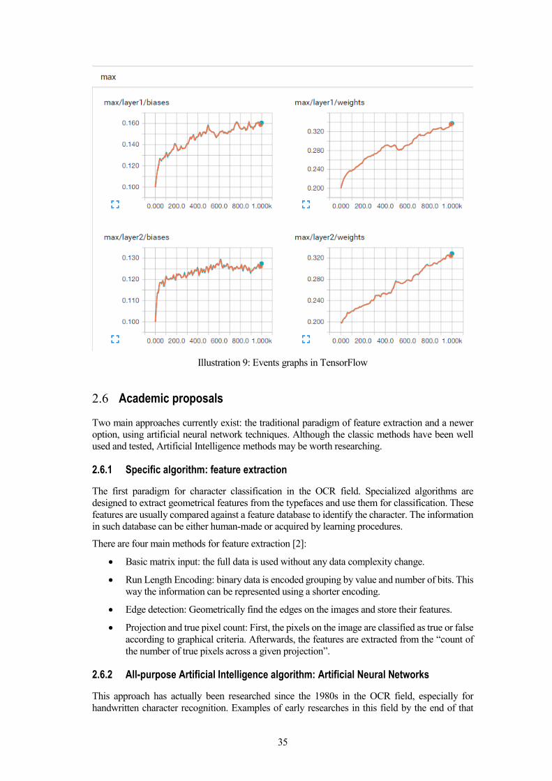
In [Illustration 9: Events graphs in TensorFlow], the graphs from the “events” tab of TensorBoard

is shown.

34

Illustration 8: TensorBoard graphs section

35

Illustration 9: Events graphs in TensorFlow

2.6 Academic proposals

Two main approaches currently exist: the traditional paradigm of feature extraction and a newer

option, using artificial neural network techniques. Although the classic methods have been well

used and tested, Artificial Intelligence methods may be worth researching.

2.6.1 Specific algorithm: feature extraction

The first paradigm for character classification in the OCR field. Specialized algorithms are

designed to extract geometrical features from the typefaces and use them for classification. These

features are usually compared against a feature database to identify the character. The information

in such database can be either human-made or acquired by learning procedures.

There are four main methods for feature extraction [2]:

Basic matrix input: the full data is used without any data complexity change.

Run Length Encoding: binary data is encoded grouping by value and number of bits. This

way the information can be represented using a shorter encoding.

Edge detection: Geometrically find the edges on the images and store their features.

Projection and true pixel count: First, the pixels on the image are classified as true or false

according to graphical criteria. Afterwards, the features are extracted from the “count of

the number of true pixels across a given projection”.

2.6.2 All-purpose Artificial Intelligence algorithm: Artificial Neural Networks

This approach has actually been researched since the 1980s in the OCR field, especially for

handwritten character recognition. Examples of early researches in this field by the end of that

36

decade can be found at [42], [43] and [44]. The first model for neural networks was developed by

Warren McCulloch and Walter Pitts in 1943 [45]. This field was researched during the 1990s but

had a boom in the 2000s due to the discovery of new learning techniques in 2006 and the

development of more advanced hardware, especially GPUs (Graphics Processor Units).

Both options are sometimes combined to get a more flexible and efficient solution. Using one

of the four feature-extraction methods above first can simplify the input to the neural network,

making it faster and easier to train.

2.6.3 Chosen option

After researching both academic options and analyzing the state of the art, the chosen alternative

is to plainly use Artificial Neural Networks, without prior feature extraction. The main reason for

this choice is the wide range of possibilities that it offers: not only character identification, but also

prediction for error correction and natural language capabilities. At feature extraction for character

classification, a big enough neural network could provide better results than expressly made

algorithms. The convolutional character of some layers would improve the results when analyzing

the images. Another advantage of neural networks is their high noise tolerance and flexibility.

In addition, deep learning techniques are being successfully used in cutting-edge technology

products and are providing promising results in many fields. While this is not a reason to use them,

it is foreseeable that these technologies keep growing up in the close future. This project would be

assured support in the future since neural network tools are expected to continue being developed

and maintained. On the contrary, classical OCR programs are beginning to suffer some degree of

decay in favor to deep learning techniques.

37

3 PROPOSED SOLUTION

solution is proposed here for the Library of the University of Seville to achieve its goals at

antique book automatic transcription.

A research at the University of Munich has used Tesseract for a similar goal with reasonable

results [46]. Nevertheless, this is the only paper addressing this very problem and very poor

results have been achieved using Tesseract on books from the XVI century in this project. The

ANN approach could be worth researching: even after an exhaustive training, Tesseract may not

be able to achieve what well trained neural networks potentially could.

Artificial Neural Networks and their variants have proved to be effective at pattern [47],

graphic and speech recognition [48], as well as at image classifying. The MNIST database is

usually used to test the efficacy of image classification algorithms. It consists in a large image set

of handwritten digits, which can be used for training and testing a classifier. The best result ever

achieved testing with this set was [49] with an error rate of 0.23%. More information is available

at the MNIST website [50]. For speech recognition a similar data set called TIMIT is used [51].

3.1 Details of the proposed solution

The solution suggested to the Library of the University of Seville consists in the development of

an OCR program using Neural Network techniques, concretely a Convolutional Neural Network.

This is convenient for classifying individual characters.

This report suggests TensorFlow as library for neural networks because of its simplicity,

efficiency and execution flexibility, as well as its future projection. Nevertheless, other open source

libraries could be also used. The solution could be a Python program during test stages, but it would

be recommendable to port it to C++ once it is definitive.

Resulting error rates should be measured using a modern adaptation of the tool presented in [52].

It would be necessary to design the layer architecture combining the elements usually used for

convolutional networks (convolutional, pooling, ReLU and fully connected layers). The

arrangement should be such that it is able to classify individual characters at least an 80% of the

times after training.

Next, the program would need to be adapted to identify more complex structures, it is whole

pages. The suggested solution involves a scale-changing sliding window. It consists in executing

the neural network over different parts of the page. In other words, using as input different subsets

of the page with different size and position. The characters will be likely to be at places where the

probability is higher at the classification phase. If one execution returns low probabilities for all

the character classes, there probably is not any letter, but noise or graphics. In addition, layers can

be inserted in order to hierarchically recognize layout entities: columns, paragraphs, lines, words

and characters.

A

38

Illustration 10: Elements detected by sliding window

After implementing a sliding window, the following task would be to provide the program with

recurrent capabilities. This capacity would be crucial to link characters into words and sentences,

due to its sensibility to past iterations.

The following task would be to study parallel and distributed computing techniques for the

OCR. The work could be split among the servers of the Library, the computing cloud offered by

the CICA and even idle work computers. In order to achieve this, it may be useful to use a

distributed file system and RPC (Remote Procedure Call) techniques or the built-in options that

TensorFlow offers. A proposal for the distributed system is available in the following subsection.

Last, it would be necessary to integrate it in the workflow of the Ancient Books Section of the

Library. It involves several topics:

Input: Scanned books must be fed to the OCR.

Output: The text output must be safely stored with the books images in the NAS (Network

Attached Storage) systems of the Library.

Distribution and publishing: The results must be made available to the public at the

website of the Library. For that, it would be necessary to index the texts so they are

searchable and integrate them with the scanned images. This could require some major

web development. ElasticSearch [53] could be a good option for content indexing and

searching, and could be easily integrated in the current websites of the Library.

The solution would then be ready for production stage and should be deployed in the Library’s

servers.

A brief project management temporal plan is included as an annex.

39

Illustration 11: Summary Gantt Chart

3.2 Distributed architecture proposal

The Library needs a distributed computation architecture to be able to process such a number of

books in its infrastructure. Two different paradigms arise for achieving this:

Distributed execution: The program is executed among different nodes in a cluster. Each

machine would be responsible of certain calculation within the neural network

architecture. TensorFlow supports both device and machine distribution [54].

Task distribution: A central machine distributes the pages of each book among the

different machines in a cluster.

The decision depends on the available infrastructure. For example, in a purpose-built

computation cluster the first option would be more convenient: distributing calculations. On the

contrary, if the process was made using casual resources such as regular server idle time, a task

distribution would limit network bandwidth use.

The following is a task distributed system proposal based on a project presented in a subject

and made with David Barranco [55].

It follows a master-slave architecture and is programmed in Go, a very efficient programming

language. It’s extremely convenient for servers and parallel computing, as well as powerful,

elegant and easy to write [56].

3.2.1 Master server

This program is at the same time a HTTP and RPC server. The HTTP API allows it to interact with

the librarian, it is to accept images and return the result. RPC enables it to communicate with slaves.

3.2.1.1 HTTP

It is a very simple server implementing two handlers to respond at two web addresses:

Upload: It admits a HTTP POST method with the image to process. It responses with the

job id assigned to the request.

State: It receives as request parameter the job id to obtain the state of. It returns the result

of the OCR execution in one of the nodes if it is ready.

Note that the CORS (Cross-Origin Resource Sharing) headers must be included in the responses

in order to allow these methods to be called from another website, it is the one that the librarians

ID Task Duration

1 Neural Network initial architecture design and documentation

28 days

2 Training set gathering 55 days

3 Convolutional Neural Network implementation

65 days

9 Sliding window implementation

85 days

16 Recurrent Neural Network Character

155 days

25 Port to C++ 55 days

31 Distributed computation 75 days

45 Workflow integration 140 days

57 Final project report and public release

15 days

58 Upkeep and incremental maintenance

163 days

M M J S N J M M J S N J M M J S N J M

Half 1, 2017 Half 2, 2017 Half 1, 2018 Half 2, 2018 Half 1, 2019 Half 2, 2019 Half 1, 2020

40

would use to upload books:

Access-Control-Allow-Credentials: true

Access-Control-Allow-Headers: Content-Type, Content-Length, Accept-Encoding, X-CSRF-Token

Access-Control-Allow-Methods: POST, GET

Access-Control-Allow-Origin: *

3.2.1.2 RPC

The methods exported for the client to use are the following:

func acceptConnection(client *rpc2.Client, args *Args_Connections, reply

*Reply_Connections) error

This method establishes connections with the client. The slaves use this method

to connect the master when they begin running to register themselves. The master

keeps all the node data in a linked list. A new element is added to the list every

time that a slave connects.

func closeConnection(client *rpc2.Client, args *Args_ Connections, reply

*Reply_ Connections) error

This method is called when a slave decides to close. The master searches the node

in the linked list and removes it, so no new jobs are assigned to them.

func receiveResponse(client *rpc2.Client, args *Args_ receiveResponse, reply

*Reply_ receiveResponse) error

Thank to this method, the master can get the result of a job when it is finished in

a node and store it, so that the result can be retrieved using the HTTP method.

3.2.2 Slave

The slaves connect to the master to provide the OCR service. It workflow is like the following:

Connect the master and register.

Wait until they are assigned a job.

Receive the image.

Call the OCR methods and synchronously wait for it to end.

Send the result back to the master.

Wait for a new job.

The only RPC method in the slave is called by the master to request a job. It receives the image to

process.

func receiveImage(client *rpc2.Client, args *Args_ receiveImage, reply

*Reply_receiveImage) error

The whole source code of the project this proposition is based upon can be found in the project

Github repository [57]. It includes both slave and master as well as a frontend interface and ANN

scripts in Python.

41

Illustration 12: Flow of information in solution structure

Librarian's tools website

Master Nodes

42

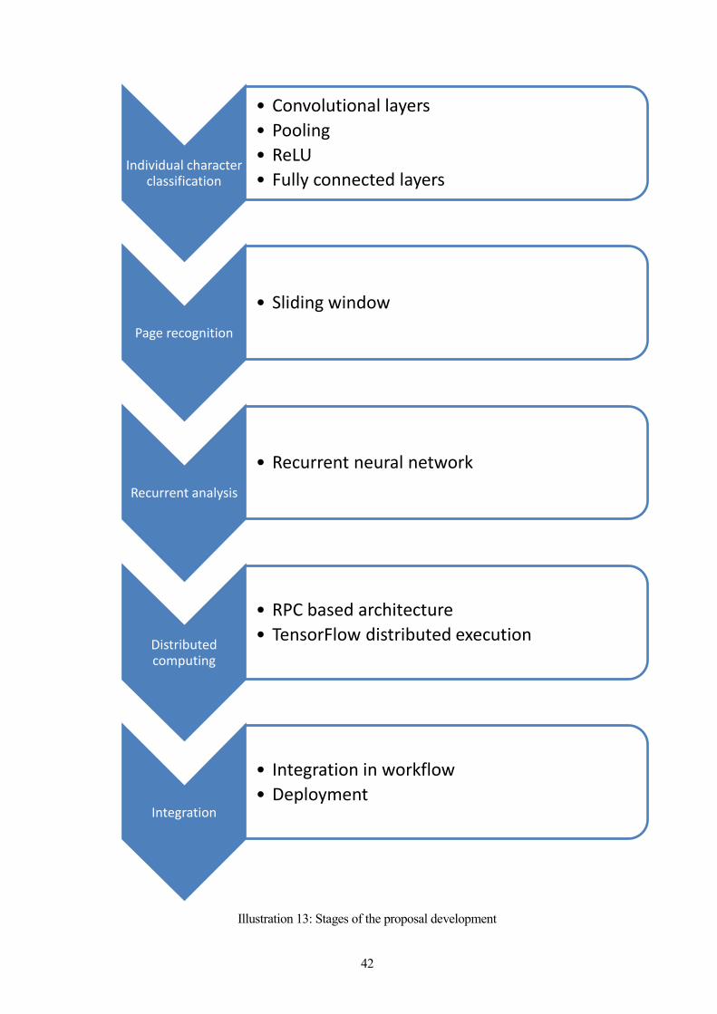
Illustration 13: Stages of the proposal development

Individual character classification

• Convolutional layers

• Pooling

• ReLU

• Fully connected layers

Page recognition

• Sliding window

Recurrent analysis

• Recurrent neural network

Distributed computing

• RPC based architecture

• TensorFlow distributed execution

Integration

• Integration in workflow

• Deployment

43

4 FIRST DRAFT AND RESULTS

s an introduction to the full proposed solution, a brief Python program has been developed

as an initial approach. TensorFlow has been used for neural networks. The full code can

be consulted at the annex and the project repository.

The program structure is based on the code used in the Udacity deep learning course [58].

4.1 Structure of the neural network

The network at this example is composed by a three convolutional layers–all followed by a

hidden layer–, a relu and a fully connected layer at the end. Finally, the softmax function gets the

probability of occurrence to each class.

The full source code can be found at the project GitHub repository:

https://github.com/Boca13/OCRFlow

# Datos de entrada como una constante de tf. tf_dataset_problema = tf.constant(dataset_problema) # Definimos el modelo. def modelo(datos): # Primera capa convolucional conv1 = tf.nn.conv2d(datos, capa1_pesos, [1, 2, 2, 1], padding='SAME') oculta1 = tf.nn.relu(conv1 + capa1_sesgos) # Segunda capa convolucional conv2 = tf.nn.conv2d(oculta1, capa2_pesos, [1, 2, 2, 1], padding='SAME') oculta2 = tf.nn.relu(conv2 + capa2_sesgos) dimensiones = oculta2.get_shape().as_list() reshape = tf.reshape(oculta2, [dimensiones[0], dimensiones[1] * dimensiones[2] * dimensiones[3]]) relu = tf.nn.relu(tf.matmul(reshape, capa3_pesos) + capa3_sesgos) # Devuelve relu * pesos4 + sesgos4 return tf.matmul(relu, capa4_pesos) + capa4_sesgos

Code 1: Detail of layer setup

A

https://github.com/Boca13/OCRFlow

44

Illustration 14: Layer architecture

4.2 Structure of the program

The OCR draft is able to classify grayscale images with a size of 28x28 pixels into ten classes:

uppercase letters from A to J. The solution has been divided in three programs:

1. Training preparation: This script compiles the training samples into a big “pickle” file,

that the next script will use to train.

2. Training: This program uses the pickle files to train the neural network in 3000 steps. At

the end it trials the just trained network with a test dataset. The trained data (weight

matrixes and bias vectors) is serialized and stored in a file.

3. Classification: Execution of the OCR on a specific image.

Illustration 15: Structure of the draft program

Classification

1. Loads trained data from previous stage2. Classifies a concrete character from a

image file, providing the certainty

Training

1. Trains the network on the example characters and saves results into a file

2. Tests the network using characters from the example dataset

Training preparation

Save dataset images into a file

Convolutional layer

Hidden layer

Convolutional layer

Hidden layer

Relu

Fully connected

layer

Softmax

45

4.3 Results of the first-approach solution

The results shown here have been obtained using the notMNIST dataset, not characters from

original antique fonts. In fact, obtaining a dataset with the target book characters is not trivial and

is a great challenge for the Library.

Illustration 16: Training iteration

4.3.1 Training preparation

This code compiles the images of each class into a file (one for each). Then

In the dataset there are two folders: the larger one has character samples meant for training; the

smaller one has fewer samples and they are supposed to be used for testing and validation.

['./grande/A', './grande/B', './grande/C', './grande/D', './grande/E',

'./grande/F', './grande/G', './grande/H', './grande/I', './grande/J']

./grande/A.pickle already present - Skipping pickling.

./grande/B.pickle already present - Skipping pickling.

./grande/C.pickle already present - Skipping pickling.

./grande/D.pickle already present - Skipping pickling.

./grande/E.pickle already present - Skipping pickling.

./grande/F.pickle already present - Skipping pickling.

./grande/G.pickle already present - Skipping pickling.

./grande/H.pickle already present - Skipping pickling.

./grande/I.pickle already present - Skipping pickling.

./grande/J.pickle already present - Skipping pickling.

./peq/A.pickle already present - Skipping pickling.

./peq/B.pickle already present - Skipping pickling.

./peq/C.pickle already present - Skipping pickling.

./peq/D.pickle already present - Skipping pickling.

./peq/E.pickle already present - Skipping pickling.

./peq/F.pickle already present - Skipping pickling.

./peq/G.pickle already present - Skipping pickling.

./peq/H.pickle already present - Skipping pickling.

./peq/I.pickle already present - Skipping pickling.

./peq/J.pickle already present - Skipping pickling.

num_classes 10

valid_size 5000

train_size 100000

vsize_per_class 500

tsize_per_class 10000

DIMENSIONES: (100000, 28, 28)

Label: 0 ; pickle_file: ./grande/A.pickle

Label: 1 ; pickle_file: ./grande/B.pickle

Label: 2 ; pickle_file: ./grande/C.pickle

Label: 3 ; pickle_file: ./grande/D.pickle

Label: 4 ; pickle_file: ./grande/E.pickle

Label: 5 ; pickle_file: ./grande/F.pickle

Label: 6 ; pickle_file: ./grande/G.pickle

Label: 7 ; pickle_file: ./grande/H.pickle

Label: 8 ; pickle_file: ./grande/I.pickle

Label: 9 ; pickle_file: ./grande/J.pickle

num_classes 10

valid_size 0

train_size 3000

vsize_per_class 0

tsize_per_class 300

DIMENSIONES: (3000, 28, 28)

Training on a test batch

Validation of the network that far

46

Label: 0 ; pickle_file: ./peq/A.pickle

Label: 1 ; pickle_file: ./peq/B.pickle

Label: 2 ; pickle_file: ./peq/C.pickle

Label: 3 ; pickle_file: ./peq/D.pickle

Label: 4 ; pickle_file: ./peq/E.pickle

Label: 5 ; pickle_file: ./peq/F.pickle

Label: 6 ; pickle_file: ./peq/G.pickle

Label: 7 ; pickle_file: ./peq/H.pickle

Label: 8 ; pickle_file: ./peq/I.pickle

Label: 9 ; pickle_file: ./peq/J.pickle

Training: (100000, 28, 28) (100000,)

Validation: (5000, 28, 28) (5000,)

Testing: (3000, 28, 28) (3000,)

Compressed pickle size: 339120441

Training: (100000, 784) (100000,)

Validation: (5000, 784) (5000,)

Testing: (3000, 784) (3000,)

Code 2: Results of the execution of preparation script

Illustration 17: Output file after training preparation

4.3.2 Training

The training script executes a loop for training the neural network. The training is done in groups

called “batches”, it is using a bunch of samples each time. The batch size has been set to 10 samples

per iteration. At each iteration, the values of the weight matrixes are changed depending on the

loss, which measures the error rate. At the end of each iteration, a small test called validation is

made in order to know the accuracy of the network so far.

“Minibatch accuracy” refers to the precision rate resulting using training characters, while

“Validation accuracy” means the accuracy rate gotten using the smaller dataset, the one meant for

training. This allows the script to know how it is doing and change the values in the matrixes

according to it. It is important to use for validation different samples than for training, since it

means to trial the network with data that it has never seen. Otherwise, the accuracy results would

not be reliable and the training could not work.

At the end of training, the script performs a test using data from the small/test dataset. The size

of the test has been set to 3000 samples. This means that the network is used to classify 3000

characters. This results in an accuracy percentage that tells how good the training was. In this case,

the accuracy obtained at test is 92.4%.

Training set (100000, 28, 28) (100000,)

Validation set (5000, 28, 28) (5000,)

Test set (3000, 28, 28) (3000,)

Training set (100000, 28, 28, 1) (100000, 10)

Validation set (5000, 28, 28, 1) (5000, 10)

Test set (3000, 28, 28, 1) (3000, 10)

Initialized

Minibatch loss at step 0: 3.427908

Minibatch accuracy: 20.0%

Validation accuracy: 10.0%










47




[...]







Test accuracy: 92.4%

Code 3: Output of the training program

Illustration 18: Serialized output file of the training program

4.3.3 Classifier

The classifier performs classification on only one character from an image file using the previously

trained data. It provides the certainty level obtained. Seven example classifications are here shown

for illustration purposes. Nevertheless, it is in the test phase that the network is properly tested.

Note that example characters from the notMNIST dataset have been used, not antique book

samples. It would be a task for the Library to obtain such dataset.

Con probabilidad 99.9578% la letra es una:

G

Code 4: Example classifier execution ("With probability 99.9578% the letter is a: \ G")

Summary of a set of seven executions on letters from the example test dataset:

Letter Image Certainty

E

99.1257%

B

99.9439%

A

99.9993%

G

99.9578%

H

97.2712%

J

99.8902%

F

99.9897%

49

5 CONCLUSION

his project could be feasible by the Library and would be a worldwide referent in antique

culture publicity and democratization, as well as an interesting contribution to the neural

networks and deep learning fields. It would provide a world recognition to the University

of Seville, positioning it at a lead position at these topics.

In addition, history researches could be done using this tool, as the data would become easier

to analyze and extract conclusions from.

It could be possible to share the project fulfillment and costs with other institutions to

maximize its probabilities of success.

In any case, it is a very interesting subject to research about and the deep learning area is

going to keep growing and provide solutions to many issues for humankind.

5.1 Future guidelines

After the draft neural network presented in this project, the next steps would be to refine it and

improve it by adding convolutional capabilities and recurrent neural network nature in order to

improve the results.

The use of a LSTM (Long Short-Term Memory) network would improve the efficacy of the

solution, since it would help offset character classification errors. That means that, even in the case

a character is wrongly classified, the resulting word may be correct thanks to context and the LSTM

feature.

5.2 Challenges

One of the most challenging issues for this project is obtaining a training dataset big enough for

the network to achieve a decent confidence level and low error rate. The minimum number of

samples needed to obtain good results is approximately 45,000, but up to 100,000 would be

recommended.

Several datasets already exist for OCR training tasks, such as the notMNIST dataset [59],

available at [60]. It is monochromatic and it covers ten classes: letters A-J. The Chars74K dataset

[61] has fewer samples but it covers 64 classes: lowercase and uppercase letters and numbers. It

can be consulted at [62].

The best option would be to create a specific dataset for training the network on the characters

of the target works. Such a dataset could be either composed out of human-tagged real samples

or computer-rendered images using a font. Nevertheless, existing sample databases could be a

good starting point for the project.

T

6 ANNEX: TRAINING TESSERACT

This annex shows how to compile Tesseract to have learning capabilities, how to use it and other

information and results

6.1 Compiling Tesseract

In order to be able to use Tesseract in a Linux system, the program can be either installed from a

Linux software repository or compiled from source, available at its GitHub repository [63]. The

second way enables for better control as well as the possibility of building the binaries necessary

for training the OCR.

A shell-script has been coded for the installation:

# Esta variable dependerá del sistema

INSTALAR="yum -yq install"

echo "Se procederá a instalar Tesseract compilando desde fuente"

read -r -p "¿Instalar herramientas de entrenamiento? [s/n]" train

echo "Instalando dependencias"

$INSTALAR git

$INSTALAR autoconf automake libtool

$INSTALAR libpng-devel

$INSTALAR libjpeg-devel

$INSTALAR libtiff-devel

$INSTALAR zlib-devel

$INSTALAR leptonica-devel

if [ "$train" = "s" ]; then

$INSTALAR libicu-devel

$INSTALAR pango-devel

$INSTALAR cairo-devel

fi

# Clonar respositorio

git clone https://github.com/tesseract-ocr/tesseract.git

cd tesseract/

# Compilar

./autogen.sh

./configure

make

52

make install

ldconfig

# Compilar entrenamiento

if [ "$train" = "s" ]; then

make training

make training-install

fi

# Idiomas

echo "Falta instalar los idiomas o entrenar al OCR"

echo "Los idiomas se pueden descargar desde

https://github.com/tesseract-ocr/tessdata"

echo "Copie los idiomas que desee a la carpeta

/usr/local/share/tessdata"

Code 5: Shell-script for automated installation of Tesseract

Once a learning file has been obtained out of the learning process, it would not be necessary to

compile the program again for the machines to execute the OCR: it would be enough to install it

from the available Linux software packets manager.

6.2 Setup and use

The syntax to exeute the OCR on a picture is the following:

tesseract image result [options] [configuration file]

The available options are the following:

Option Function

--tessdata-dir PATH Specifies the data folder for Tesseract (usually

/usr/local/share/tessdata)

--user-words PATH Specifies the location of the user lexicon file

--user-patterns PATH Specifies the location of the user patterns

(substitutions) file

-l LANGUAGE[+LANG] Specifies the language(s) to be used by the OCR

-c VARIABLE=VALUE Sets the value of configuration variable(s)

-psm NUMBER Sets the page segmentation mode

53

The available page segmentation modes are:

0 Orientation and script detection (OSD) only.

1 Automatic page segmentation with OSD.

2 Automatic page segmentation, but no OSD, or OCR.

3 Fully automatic page segmentation, but no OSD. (Default)

4 Assume a single column of text of variable sizes.

5 Assume a single uniform block of vertically aligned text.

6 Assume a single uniform block of text.

7 Treat the image as a single text line.

8 Treat the image as a single word.

9 Treat the image as a single word in a circle.

10 Treat the image as a single character.

This OCR has worked successfully at trials with contemporary texts in several languages.

6.3 Training

Training the OCR allows it to improve the score in most of cases. This training consists in creating

a new “traineddata” file by following a sequence of steps. These steps are described at the Tesseract

repository [64] and are here summarized:

Render images out of an example text. The advantage of doing so is that a correct “box”

file is generated. This way, the human correction phase is avoided, but a font file is

needed. The command text2image is used.

Execute Tesseract in learning mode. This generates a .tr file, which contains the features

of each character.

Calculate the character set using the command unicharset_extractor, which

generates a file with all the characters that the OCR will be able to detect.

Execute the command set_unicharset_properties, which gives more information

about the font. It is added to the character set.

Create a file with font information.

Group everything to create prototypes. The programs mftraining and cntraining

are used.

Optionally, add lexicon data.

Create a substitutions file named unicharambigs. This file makes possible to define

mandatory or optional substitutions which will be done once the images are processed.

Finally, compile everything in the same file with the command combine_tessdata.

The total training execution time depends strongly on the number of samples.

7 ANNEX: CODE OF THE INITIAL OCR

This is the code of the first draft, an introduction to the full proposed solution able to recognize

characters from A to J from images with a size of 28x28 pixels.

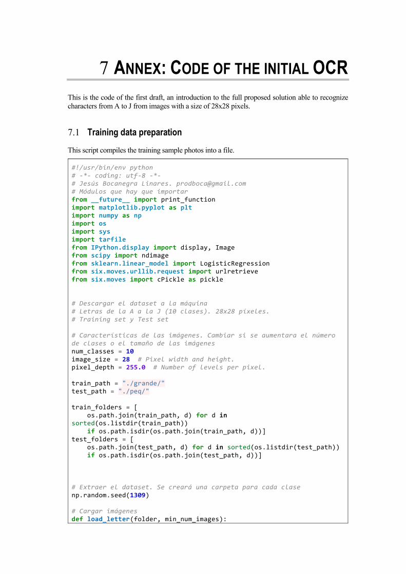
7.1 Training data preparation

This script compiles the training sample photos into a file.

#!/usr/bin/env python # -*- coding: utf-8 -*- # Jesús Bocanegra Linares. [email protected] # Módulos que hay que importar from __future__ import print_function import matplotlib.pyplot as plt import numpy as np import os import sys import tarfile from IPython.display import display, Image from scipy import ndimage from sklearn.linear_model import LogisticRegression from six.moves.urllib.request import urlretrieve from six.moves import cPickle as pickle # Descargar el dataset a la máquina # Letras de la A a la J (10 clases). 28x28 píxeles. # Training set y Test set # Características de las imágenes. Cambiar si se aumentara el número de clases o el tamaño de las imágenes num_classes = 10 image_size = 28 # Pixel width and height. pixel_depth = 255.0 # Number of levels per pixel. train_path = "./grande/" test_path = "./peq/" train_folders = [ os.path.join(train_path, d) for d in sorted(os.listdir(train_path)) if os.path.isdir(os.path.join(train_path, d))] test_folders = [ os.path.join(test_path, d) for d in sorted(os.listdir(test_path)) if os.path.isdir(os.path.join(test_path, d))] # Extraer el dataset. Se creará una carpeta para cada clase np.random.seed(1309) # Cargar imágenes def load_letter(folder, min_num_images):

56

"""Load the data for a single letter label.""" image_files = os.listdir(folder) dataset = np.ndarray(shape=(len(image_files), image_size, image_size), dtype=np.float32) image_index = 0 print(folder) for image in os.listdir(folder): image_file = os.path.join(folder, image) try: image_data = (ndimage.imread(image_file).astype(float) - pixel_depth / 2) / pixel_depth if image_data.shape != (image_size, image_size): raise Exception('Unexpected image shape: %s' % str(image_data.shape)) dataset[image_index, :, :] = image_data image_index += 1 except IOError as e: print('Could not read:', image_file, ':', e, '- it\'s ok, skipping.') num_images = image_index dataset = dataset[0:num_images, :, :] if num_images < min_num_images: raise Exception('Many fewer images than expected: %d < %d' % (num_images, min_num_images)) print('Tensor del dataset completo:', dataset.shape) print('Media:', np.mean(dataset)) print('Desviación típica:', np.std(dataset)) return dataset def maybe_pickle(data_folders, min_num_images_per_class, force=False): dataset_names = [] for folder in data_folders: set_filename = folder + '.pickle' dataset_names.append(set_filename) if os.path.exists(set_filename) and not force: print('%s already present - Skipping pickling.' % set_filename) else: print('Pickling %s.' % set_filename) dataset = load_letter(folder, min_num_images_per_class) try: with open(set_filename, 'wb') as f: pickle.dump(dataset, f, pickle.HIGHEST_PROTOCOL) except Exception as e: print('Unable to save data to', set_filename, ':', e) return dataset_names print(train_folders) train_datasets = maybe_pickle(train_folders, 1000) test_datasets = maybe_pickle(test_folders, 100) # Tratar los datos def make_arrays(nb_rows, img_size): if nb_rows: dataset = np.ndarray((nb_rows, img_size, img_size), dtype=np.float32)

57

labels = np.ndarray(nb_rows, dtype=np.int32) else: dataset, labels = None, None return dataset, labels def merge_datasets(pickle_files, train_size, valid_size=0): num_classes = len(pickle_files) valid_dataset, valid_labels = make_arrays(valid_size, image_size) train_dataset, train_labels = make_arrays(train_size, image_size) vsize_per_class = valid_size // num_classes tsize_per_class = train_size // num_classes print("num_classes", num_classes) print("valid_size", valid_size) print("train_size", train_size) print("vsize_per_class", vsize_per_class) print("tsize_per_class", tsize_per_class) print("DIMENSIONES: ", train_dataset.shape) start_v, start_t = 0, 0 end_v, end_t = vsize_per_class, tsize_per_class end_l = vsize_per_class+tsize_per_class for label, pickle_file in enumerate(pickle_files): print("Label: ", label, "; pickle_file: ", pickle_file) try: with open(pickle_file, 'rb') as f: letter_set = pickle.load(f) # Mezclar las letras para que los juegos de validación y prueba sean aleatorios np.random.shuffle(letter_set) if valid_dataset is not None: valid_letter = letter_set[:vsize_per_class, :, :] valid_dataset[start_v:end_v, :, :] = valid_letter valid_labels[start_v:end_v] = label start_v += vsize_per_class end_v += vsize_per_class train_letter = letter_set[vsize_per_class:end_l, :, :] train_dataset[start_t:end_t, :, :] = train_letter train_labels[start_t:end_t] = label start_t += tsize_per_class end_t += tsize_per_class except Exception as e: print('Unable to process data from', pickle_file, ':', e) raise return valid_dataset, valid_labels, train_dataset, train_labels train_size = 100000 valid_size = 5000 test_size = 3000 valid_dataset, valid_labels, train_dataset, train_labels = merge_datasets( train_datasets, train_size, valid_size) _, _, test_dataset, test_labels = merge_datasets(test_datasets, test_size)

58

print('Training:', train_dataset.shape, train_labels.shape) print('Validation:', valid_dataset.shape, valid_labels.shape) print('Testing:', test_dataset.shape, test_labels.shape) # Aleatorizar datos def randomize(dataset, labels): permutation = np.random.permutation(labels.shape[0]) shuffled_dataset = dataset[permutation,:,:] shuffled_labels = labels[permutation] return shuffled_dataset, shuffled_labels train_dataset, train_labels = randomize(train_dataset, train_labels) test_dataset, test_labels = randomize(test_dataset, test_labels) valid_dataset, valid_labels = randomize(valid_dataset, valid_labels) # Guardar datos pickle_file = 'data.pickle' try: f = open(pickle_file, 'wb') save = { 'train_dataset': train_dataset, 'train_labels': train_labels, 'valid_dataset': valid_dataset, 'valid_labels': valid_labels, 'test_dataset': test_dataset, 'test_labels': test_labels, } pickle.dump(save, f, pickle.HIGHEST_PROTOCOL) f.close() except Exception as e: print('Unable to save data to', pickle_file, ':', e) raise statinfo = os.stat(pickle_file) print('Compressed pickle size:', statinfo.st_size) ##RESHAPE!! train_dataset = np.array(train_dataset) train_labels = np.array(train_labels) train_dataset = train_dataset.reshape((train_size,image_size*image_size)); valid_dataset = valid_dataset.reshape((valid_size,image_size*image_size)); test_dataset = test_dataset.reshape((test_size,image_size*image_size)); print('Training:', train_dataset.shape, train_labels.shape) print('Validation:', valid_dataset.shape, valid_labels.shape) print('Testing:', test_dataset.shape, test_labels.shape)

Code 6: Training data preparation

59

7.2 Training code

This code trains the network and saves the parameters (weights and biases) to a file:

#!/usr/bin/env python # -*- coding: utf-8 -*- # Jesús Bocanegra Linares. [email protected] # Módulos que hay que importar from __future__ import print_function import numpy as np import tensorflow as tf import sys from scipy import ndimage from six.moves import cPickle as pickle from six.moves import range # Reformatear para que tenga una forma comaptible con TensorFlow # - Las convoluciones necesitan los datos de imagen formateados como un cubo (ancho x alto x número de canales) # - Las etiquetas son decimales (float) en codificación 1-hot. image_size = 28 num_labels = 10 num_channels = 1 # escala de grises import numpy as np pickle_file = 'data.pickle' with open(pickle_file, 'rb') as f: save = pickle.load(f) train_dataset = save['train_dataset'] train_labels = save['train_labels'] valid_dataset = save['valid_dataset'] valid_labels = save['valid_labels'] test_dataset = save['test_dataset'] test_labels = save['test_labels'] del save # Liberar memoria print('Training set', train_dataset.shape, train_labels.shape) print('Validation set', valid_dataset.shape, valid_labels.shape) print('Test set', test_dataset.shape, test_labels.shape) def reformat(dataset, labels): dataset = dataset.reshape( (-1, image_size, image_size, num_channels)).astype(np.float32) labels = (np.arange(num_labels) == labels[:,None]).astype(np.float32) return dataset, labels train_dataset, train_labels = reformat(train_dataset, train_labels) valid_dataset, valid_labels = reformat(valid_dataset, valid_labels) test_dataset, test_labels = reformat(test_dataset, test_labels) print('Training set', train_dataset.shape, train_labels.shape) print('Validation set', valid_dataset.shape, valid_labels.shape) print('Test set', test_dataset.shape, test_labels.shape)

60

def accuracy(predictions, labels): return (100.0 * np.sum(np.argmax(predictions, 1) == np.argmax(labels, 1)) / predictions.shape[0]) batch_size = 10 patch_size = 5 depth = 16 num_hidden = 64 graph = tf.Graph() with graph.as_default(): # Input data. tf_train_dataset = tf.placeholder( tf.float32, shape=(batch_size, image_size, image_size, num_channels)) tf_train_labels = tf.placeholder(tf.float32, shape=(batch_size, num_labels)) tf_valid_dataset = tf.constant(valid_dataset) tf_test_dataset = tf.constant(test_dataset) # Define variables that will hold the trained parameters and will be used for classifiying layer1_weights = tf.Variable(tf.truncated_normal( [patch_size, patch_size, num_channels, depth], stddev=0.1)) layer1_biases = tf.Variable(tf.zeros([depth])) layer2_weights = tf.Variable(tf.truncated_normal( [patch_size, patch_size, depth, depth], stddev=0.1)) layer2_biases = tf.Variable(tf.constant(1.0, shape=[depth])) layer3_weights = tf.Variable(tf.truncated_normal( [image_size // 4 * image_size // 4 * depth, num_hidden], stddev=0.1)) layer3_biases = tf.Variable(tf.constant(1.0, shape=[num_hidden])) layer4_weights = tf.Variable(tf.truncated_normal( [num_hidden, num_labels], stddev=0.1)) layer4_biases = tf.Variable(tf.constant(1.0, shape=[num_labels])) # Model. def model(data): conv = tf.nn.conv2d(data, layer1_weights, [1, 2, 2, 1], padding='SAME') hidden = tf.nn.relu(conv + layer1_biases) conv2 = tf.nn.conv2d(hidden, layer2_weights, [1, 2, 2, 1], padding='SAME') hidden = tf.nn.relu(conv2 + layer2_biases) shape = hidden.get_shape().as_list() reshape = tf.reshape(hidden, [shape[0], shape[1] * shape[2] * shape[3]]) hidden = tf.nn.relu(tf.matmul(reshape, layer3_weights) + layer3_biases) return tf.matmul(hidden, layer4_weights) + layer4_biases # Training computation. logits = model(tf_train_dataset) loss = tf.reduce_mean(

61

tf.nn.softmax_cross_entropy_with_logits(logits, tf_train_labels)) # Optimizer. optimizer = tf.train.GradientDescentOptimizer(0.1).minimize(loss) # Predictions for the training and validation train_prediction = tf.nn.softmax(logits) valid_prediction = tf.nn.softmax(model(tf_valid_dataset)) test_prediction = tf.nn.softmax(model(tf_test_dataset)) num_steps = 3001 with tf.Session(graph=graph) as session: tf.initialize_all_variables().run() print('Initialized') for step in range(num_steps): offset = (step * batch_size) % (train_labels.shape[0] - batch_size) batch_data = train_dataset[offset:(offset + batch_size), :, :, :] batch_labels = train_labels[offset:(offset + batch_size), :] feed_dict = {tf_train_dataset : batch_data, tf_train_labels : batch_labels} _, l, predictions = session.run([optimizer, loss, train_prediction], feed_dict=feed_dict) if (step % 50 == 0): print('Minibatch loss at step %d: %f' % (step, l)) print('Minibatch accuracy: %.1f%%' % accuracy(predictions, batch_labels)) print('Validation accuracy: %.1f%%' % accuracy(valid_prediction.eval(), valid_labels)) print("Test accuracy: %.1f%%" % accuracy(test_prediction.eval(), test_labels)) # Guardar entrenamiento try: with open("trained.bin", 'wb') as f: learnt = [layer1_weights.eval(session=session), layer1_biases.eval(session=session), layer2_weights.eval(session=session), layer2_biases.eval(session=session), layer3_weights.eval(session=session), layer3_biases.eval(session=session), layer4_weights.eval(session=session), layer4_biases.eval(session=session)] pickle.dump(learnt, f, pickle.HIGHEST_PROTOCOL) except Exception as e: print('Unable to save trained data', e)

Code 7: Training

7.3 Character classification

The code to identify a character from a given picture, it is the OCR work.

#!/usr/bin/env python # -*- coding: utf-8 -*- # Jesús Bocanegra Linares. [email protected]

62

# Módulos necesarios from __future__ import print_function import numpy as np import tensorflow as tf import sys import numpy as np from scipy import ndimage from six.moves import cPickle as pickle from six.moves import range # Para redimensionar: # - las convoluciones necesitan los datos de imagen formateados como un cubo (ancho x alto x número de canales) # - las etiquetas deben ser floats y codificadas en 1-hot. tam_imagen = 28 n_clases = 10 n_canales = 1 # escala de grises profundidad_pixel = 255.0 def cargar_letra(): dataset = np.ndarray(shape=(1, tam_imagen, tam_imagen), dtype=np.float32) indice_imagen = 0 ruta_imagen = "letra.png" try: imagen = (ndimage.imread(ruta_imagen).astype(float) - profundidad_pixel / 2) / profundidad_pixel if imagen.shape != (tam_imagen, tam_imagen): raise Exception('Unexpected image shape: %s' % str(imagen.shape)) except IOError as e: print('No se pudo abrir: ', ruta_imagen, ':', e, '. Saltando.') return imagen clases = ['A', 'B', 'C', 'D', 'E', 'F', 'G', 'H', 'I', 'J'] with open('trained.bin', 'rb') as f: entrenado = pickle.load(f) # Cargar datos entrenados capa1_pesos = entrenado[0] capa1_sesgos = entrenado[1] capa2_pesos = entrenado[2] capa2_sesgos = entrenado[3] capa3_pesos = entrenado[4] capa3_sesgos = entrenado[5] capa4_pesos = entrenado[6] capa4_sesgos = entrenado[7] dataset_problema = cargar_letra() def reformat(dataset, etiquetas): dataset = dataset.reshape((-1, tam_imagen, tam_imagen, n_canales)).astype(np.float32) etiquetas = (np.arange(n_clases) == etiquetas[:,None]).astype(np.float32) return dataset, etiquetas dataset_problema = dataset_problema.reshape((-1, tam_imagen, tam_imagen, n_canales)).astype(np.float32)

63

def accuracy(predictions, etiquetas): return (100.0 * np.sum(np.argmax(predictions, 1) == np.argmax(etiquetas, 1)) / predictions.shape[0]) # Pequeña red con varias capas convolucionales seguidas de una capa completamente conectada. # Limitamos la profundidad y el número de nodos conectados, porque las redes convolucionales conllevan un alto coste computacional. tam_lote = 10 tam_parche = 5 # Gráfica por defecto: graph = tf.Graph() with graph.as_default(): # Datos de entrada como una constante de tf. tf_dataset_problema = tf.constant(dataset_problema) # Definimos el modelo. def modelo(datos): # Primera capa convolucional conv1 = tf.nn.conv2d(datos, capa1_pesos, [1, 2, 2, 1], padding='SAME') oculta1 = tf.nn.relu(conv1 + capa1_sesgos) # Segunda capa convolucional conv2 = tf.nn.conv2d(oculta1, capa2_pesos, [1, 2, 2, 1], padding='SAME') oculta2 = tf.nn.relu(conv2 + capa2_sesgos) dimensiones = oculta2.get_shape().as_list() reshape = tf.reshape(oculta2, [dimensiones[0], dimensiones[1] * dimensiones[2] * dimensiones[3]]) oculta3 = tf.nn.relu(tf.matmul(reshape, capa3_pesos) + capa3_sesgos) # Devuelve oculta3 * pesos4 + sesgos4 return tf.matmul(oculta3, capa4_pesos) + capa4_sesgos # Prediction: prediccion_problema = tf.nn.softmax(modelo(tf_dataset_problema)) with tf.Session(graph=graph) as session: tf.initialize_all_variables().run() resultado = np.array(prediccion_problema.eval()) print('Con probabilidad %f%% la letra es una: ' % resultado.max()*100) sys.exit(clases[resultado.argmax()])

Code 8: Classifier

64

8 ANNEX: PROJECT PLANNING

The proposed project planning is estimated for a three-year total duration. The project would be

executed by a junior Telecommunications Technic engineer or Computer Scientist with some

demonstrable knowledge and experience on the field. The designed person should also have

experience working with librarians and librarianship topics.

8.1 Project cost

The estimated cost for the project is the one related to the engineer’s salary. The amount is

calculated for a 13€/h rate during a three-year period, 8 hours a day. This hourly rate would mean

a 1456€ salary after taxes.

Hourly rate Annual salary Monthly salary after taxes Social security tax Total cost per year

13,00 € 29.120,00 € 1.456,00 € 9.609,60 € 38.729,60 €

Total project cost: 116.188,80 €

Project risks like tax rate changes should be considered.

8.1.1 Cost details

Name Cost Duration Work Start Finish

Neural Network

initial architecture

design and

documentation

4.518,08 € 28 days 224 hours Wed

01/03/17

Fri

07/04/17

Training set

gathering

0,00 € 55 days 0 hours Wed

01/03/17

Tue

16/05/17

Convolutional

Neural Network

implementation

10.488,40 € 65 days 520 hours Mon

10/04/17

Fri

07/07/17

Sliding window

implementation

13.715,60 € 85 days 680 hours Mon

10/07/17

Fri

03/11/17

Recurrent Neural

Network Character

25.010,80 € 155 days 1.240

hours

Mon

06/11/17

Fri

08/06/18

Port to C++ 8.874,80 € 55 days 440 hours Mon

11/06/18

Fri

24/08/18

Distributed 12.102,00 € 75 days 600 hours Mon Fri

65

computation 27/08/18 07/12/18

Workflow

integration

22.590,40 € 140 days 1.120

hours

Mon

10/12/18

Fri

21/06/19

Final project report

and public release

2.420,40 € 15 days 120 hours Mon

24/06/19

Fri

12/07/19

Upkeep and

incremental

maintenance

26.301,68 € 163 days 1.304

hours

Wed

17/07/19

Fri

28/02/20

Note that the task “Training set gathering” is expected to be performed by librarians.

8.2 Time planning

A Gantt diagram is provided below for the estimated project time planning with example dates

ranging from 2017/03/1 to 2020/02/28.

ID Task Duration Start End Predecessors

1 Neural Network initial architecture design and documentation

28 days Wed 01/03/17 Fri 07/04/17

2 Training set gathering 55 days Wed 01/03/17 Tue 16/05/17

3 Convolutional Neural Network implementation

65 days Mon 10/04/17 Fri 07/07/17 1

4 Coding 30 days Mon 10/04/17 Fri 19/05/17

5 Training 15 days Mon 22/05/17 Fri 09/06/17 4;2

6 Testing 5 days Mon 12/06/17 Fri 16/06/17 5

7 Code review and refinement after test results

10 days Mon 19/06/17 Fri 30/06/17 6

8 Documentation 5 days Mon 03/07/17 Fri 07/07/17 7

9 Sliding window implementation

85 days Mon 10/07/17 Fri 03/11/17 3

10 Software design 10 days Mon 10/07/17 Fri 21/07/17

11 Coding 30 days Mon 24/07/17 Fri 01/09/17 10


13 Learning 15 days Mon 18/09/17 Fri 06/10/17 12

14 Review 10 days Mon 09/10/17 Fri 20/10/17 13


16 Recurrent Neural Network Character

155 days Mon 06/11/17 Fri 08/06/18 9

17 Architecture Design 30 days Mon 06/11/17 Fri 15/12/17


19 Adapting training set 20 days Mon 05/02/18 Fri 02/03/18 18

20 Training 20 days Mon 05/03/18 Fri 30/03/18 19


22 Review 15 days Mon 23/04/18 Fri 11/05/18 21

23 Parameter adjusting 10 days Mon 14/05/18 Fri 25/05/18 22


M A M J J A S O N D J F M A M J J

Half 1, 2017 Half 2, 2017 Half 1, 2018 Half 2, 2018

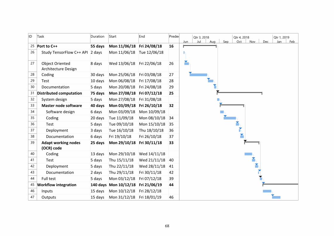
68


25 Port to C++ 55 days Mon 11/06/18 Fri 24/08/18 16

26 Study TensorFlow C++ API 2 days Mon 11/06/18 Tue 12/06/18

27 Object Oriented Architecture Design

8 days Wed 13/06/18 Fri 22/06/18 26


29 Test 10 days Mon 06/08/18 Fri 17/08/18 28


31 Distributed computation 75 days Mon 27/08/18 Fri 07/12/18 25

32 System design 5 days Mon 27/08/18 Fri 31/08/18

33 Master node software 40 days Mon 03/09/18 Fri 26/10/18 32

34 Software design 6 days Mon 03/09/18 Mon 10/09/18

35 Coding 20 days Tue 11/09/18 Mon 08/10/18 34

36 Test 5 days Tue 09/10/18 Mon 15/10/18 35

37 Deployment 3 days Tue 16/10/18 Thu 18/10/18 36

38 Documentation 6 days Fri 19/10/18 Fri 26/10/18 37

39 Adapt working nodes (OCR) code

25 days Mon 29/10/18 Fri 30/11/18 33

40 Coding 13 days Mon 29/10/18 Wed 14/11/18

41 Test 5 days Thu 15/11/18 Wed 21/11/18 40

42 Deployment 5 days Thu 22/11/18 Wed 28/11/18 41

43 Documentation 2 days Thu 29/11/18 Fri 30/11/18 42

44 Full test 5 days Mon 03/12/18 Fri 07/12/18 39

45 Workflow integration 140 days Mon 10/12/18 Fri 21/06/19 44

46 Inputs 15 days Mon 10/12/18 Fri 28/12/18

47 Outputs 15 days Mon 31/12/18 Fri 18/01/19 46

Jun Jul Aug Sep Oct Nov Dec Jan Feb

Qtr 2, 2018 Qtr 3, 2018 Qtr 4, 2018 Qtr 1, 2019

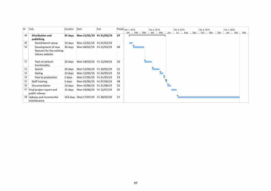
69


48 Distribution and publishing

95 days Mon 21/01/19 Fri 31/05/19 47

49 ElasticSearch setup 10 days Mon 21/01/19 Fri 01/02/19

50 Development of new features for the existing Library website

30 days Mon 04/02/19 Fri 15/03/19 49

51 Text on-picture functionality

20 days Mon 18/03/19 Fri 12/04/19 50

52 Search 20 days Mon 15/04/19 Fri 10/05/19 51

53 Styling 10 days Mon 13/05/19 Fri 24/05/19 52

54 Pass to production 5 days Mon 27/05/19 Fri 31/05/19 53

55 Staff training 5 days Mon 03/06/19 Fri 07/06/19 48


57 Final project report and public release

15 days Mon 24/06/19 Fri 12/07/19 45

58 Upkeep and incremental maintenance

163 days Wed 17/07/19 Fri 28/02/20 57

Jan Feb Mar Apr May Jun Jul Aug Sep Oct Nov Dec Jan Feb Mar

Qtr 1, 2019 Qtr 2, 2019 Qtr 3, 2019 Qtr 4, 2019 Qtr 1, 2020

9 SUMMARY IN SPANISH / RESUMEN EN

ESPAÑOL

a Biblioteca de la Universidad de Sevilla atesora una rica colección de obras antiguas que están

siendo digitalizadas. Para hacer el acceso a la información más fácil, se necesitaría el texto completo

de estos libros. Se busca encontrar una solución para su transcripción automática, ya que llevaría

mucho tiempo hacerlo a personas. Para conseguirlo, se analizan las soluciones existentes: desde programas

de código abierto con largas trayectorias a la última tecnología en redes neuronales. Tras la investigación,

se proporcionará una solución concreta para la Biblioteca, así como directrices para su ejecución.

9.1 Introducción y objetivos

Las herramientas de OCR (Reconocimiento Óptica de Caracteres) se han desarrollado desde la década de

1980 para afrontar el desafío de transcribir texto automáticamente. Este proceso consiste en adquirir una

representación textual digital a partir de un texto impreso almacenado digitalmente en una imagen.

Las ventajas de tener transcripciones digitales de contenidos escritos son numerosas y bien conocidas:

preservación de la información, disponibilidad de los datos, facilidad de traducción, búsqueda y análisis

automáticos etc.

9.1.1 Motivación

El Fondo Antiguo de la Universidad de Sevilla alberga más de 100.406 obras de un valor incalculable, de

las cuales 332 son incunables y 9.941 son del siglo XVI. Cada día, varios de estos libros se escanean en los

talleres del Fondo Antiguo y se estima que 9.500 de ellos ya han sido digitalizados.

Estas imágenes y los metadatos de los libros se publican en un portal web. Disponer de las

transcripciones, permitiría opciones muy interesantes para los investigadores y otros públicos: análisis

léxicos, indexación de los contenidos; para por ejemplo poder buscar en ellos; y estudios históricos, como

meteorológicos o demográficos.

Resulta especialmente notable la indización de los textos en una base de datos ya que permitiría que la

información de estos libros estuviera fácilmente accesible en Internet. Esto se traduciría en una verdadera

democratización de la información custodiada por la Biblioteca, ya que cualquier usuario con una conexión

a Internet podría acceder a la información aun sin tener formación específica.

9.1.2 Dificultades especiales con libros antiguos

Los algoritmos de OCR actuales funcionan correctamente con textos modernos y proporcionan una tasa de

aciertos razonable. Sin embargo, las obras más interesantes del Fondo Antiguo de la Biblioteca son de los

siglos XV a XVIII. Estos libros suponen una mayor dificultad comparados con las impresiones del siglo

XIX en adelante.

Los obstáculos más comunes para la transcripción automática son los siguientes:

Dependencia del estado de conservación del libro.

Variabilidad de las grafías: Los tipos usados en las impresiones varían según la obra y el siglo.

Heterogeneidad del idioma: La mayoría de los libros de interés están escritos en castellano antiguo,

de un tiempo en el que la ortografía no se había fijado. Esto impide usar un diccionario para

corregir errores de transcripción.

L

72

Otras características especiales de las impresiones antiguas: Las abreviaturas y ligaduras también

afectan negativamente a las transcripciones y suponen un desafío para el desarrollo.

Para el desarrollo del proyecto, sería necesario abordar temáticas de diferentes campos:

Historia de las tipografías y la imprenta.

Diplomática: reglas de transcripción.

Abreviaturas, acortamientos y caracteres especiales; todos frecuentes en los textos de los siglos de

estudio.

9.1.3 Propósito del proyecto

El objetivo de este trabajo es explorar diferentes soluciones de OCR y ayudar a la Biblioteca de la

Universidad de Sevilla a conseguir la transcripción de libros antiguos en su propia infraestructura.

Respecto a los requisitos, la propuesta sólo puede usar software libre o tecnologías de uso libre; nunca

requerir una licencia de pago. Otra condición es que el proceso debe ser viable usando solamente los

recursos de la Biblioteca. No obstante, también sería posible aceptar ayuda de otras instituciones públicas.

Por ejemplo, el CICA (Centro Informático Científico de Andalucía) ha ofrecido una parte significativa de

su clúster de computación.

Los pasos que se tomarán para conseguir el proyecto son:

1. Investigación bibliográfica sobre las soluciones de OCR existentes y otras tecnologías que podrían

ser útiles para el proyecto.

2. Se escogerán dos posibilidades de las encontradas. A continuación, se investigará su uso y se

intentará obtener resultados usándolas sobre los libros objetivo.

3. Tras ello, se propondrá una solución considerando toda la investigación. Se proporcionarán unas

pautas para que la Biblioteca pueda conseguir sus objetivos en cuanto a la transcripción de libros.

4. Por último, se presentará un borrador o primera aproximación de la solución propuesta y sus

resultados, así como las conclusiones.

Usando este informe, la Biblioteca podría ser capaz de estudiar la viabilidad y tomar decisiones sobre el

proyecto basándose en la información técnica aquí presente.

9.2 Estado del arte

Actualmente existen muchas aplicaciones de OCR. Estas soluciones suelen usar algoritmos específicos, es

decir, procedimientos específicamente diseñados para el análisis de texto. Estos métodos suelen extraer

características geométricas de las letras para clasificarlas.

Otro esquema consiste en usar técnicas de inteligencia artificial y Machine Learning más novedosas. Estas

tecnologías, como el Deep Learning están produciendo resultados a nivel de estado del arte en tareas como

visión artificial, reconocimiento del habla y procesamiento de lenguaje natural.

9.2.1 Visión de conjunto de OCR existentes

9.2.1.1 Software propietario

Adobe Acrobat

ABBYY FineReader

Asprise OCR

OmniPage

73

9.2.1.2 Soluciones gratuitas

Tesseract

CuneiForm

GOCR

Ocrad

OCRopus

9.2.2 Tesseract OCR

Tesseract es un motor OCR desarrollado en Hewlett-Packard (HP) de 1984 a 1994. Empezó como una tesis

doctoral en la Universidad de Bristol, publicada en 1987. El desarrollo del proyecto terminó en 1994. Al

año siguiente se presentó en la Prueba Anual de Precisión de OCR, donde tuvo buenos resultados respecto

a las soluciones comerciales existentes por entonces.

El proyecto se congeló hasta 2015, cuando HP decidió liberarlo como código abierto. Google

principalmente tomó las riendas del proyecto. Una de las características más interesantes de este OCR es

su capacidad de aprendizaje. Tras seguir un proceso de entrenamiento, Tesseract puede mejorar

clasificando textos de una fuente determinada.

9.2.3 Redes Neuronales Artificiales

Las redes neuronales son un paradigma de programación basado en las neuronas cerebrales. Esta solución

inspirada biológicamente permite a los ordenadores aprender de información experimental.

Se puede usar una estrategia de extracción jerárquica de características para hacer que una máquina

pueda entender datos complejos como lo hacen las personas. Esto se consigue dividiendo los problemas

complejos en partes más pequeñas usando una estructura de varias capas con un nivel de complejidad

progresivo.

Las capas se componen de neuronas artificiales. Cada neurona hace un cálculo muy simple, pero el

efecto total entre todas ellas produce el resultado buscado.

9.2.3.1 Neuronas artificiales

Una neurona artificial consiste en un conjunto de entradas y una salida relacionadas por una operación

matemática simple. Un grupo de neuronas interconectadas forma una capa.

Illustration 19: Estructura de una neurona

Las neuronas tienen las siguientes características:

Las entradas y salidas son números decimales en el intervalo (0, 1). Esto es particularmente útil

Función de

transferencia

Salida (y)

Entrada 1 (x1)

Entrada i (xi)

Entrada n (xn)

74

porque se pueden interpretar como probabilidades.

La función de transferencia, esto es la función matemática que relaciona entradas y salidas, es

como la siguiente:

y = f(W ⋅ x + b) Donde:

o y es la salida de la neurona.

o f denota la función de transferencia.

o W representa la matriz de pesos.

o x es un vector con la entrada a la neurona.

o b significa un vector con los valores de sesgo.

En resumen, la salida de cada neurona es la función de transferencia de una combinación lineal de las

entradas. En esta combinación lineal, la matriz de pesos (W) contiene los términos multiplicativos y el

vector de sesgos tiene los términos aditivos.

9.2.3.2 Funciones de transferencia

Hay dos tipos de funciones de transferencia ampliamente usadas para las neuronas:

Función logística: Es una función sigmoidea definida como:

σ(x) ≡1

1 + 𝑒−𝑥

Función rectificadora: Se trata de la función rampa:

𝑟(𝑥) = max(0, 𝑥)

9.2.3.3 Capas

Cada capa en una red neuronal es un conjunto de neuronas interconectadas. Las arquitecturas multicapa

proporcionan buenos resultados según distintos estudios. Las estructuras multicapa se identifican con un

proceso de aprendizaje jerárquico. En cada capa, se aprende y reconoce un rasgo diferente, lo que lleva a

una jerarquía de representaciones con nivel de abstracción creciente. Las capas que conectan las de entrada

y salida se llaman capas completamente conectadas.

75

Illustration 20: Red neuronal con dos capas ocultas. Por Michael Nielsen, bajo licencia CC BY-NC 3.0.

9.2.3.4 Tipos de redes neuronales

Existen algunas variantes de las redes neuronales, como las Redes Neuronales Convolucionales y las Redes

Neuronales recurrentes. Se puede hacer también una combinación de ellas.

Redes neuronales convolucionales: Se caracterizan por la presencia de capas convolutivas, cuyo

propósito es detectar rasgos visuales. La clave es que estas neuronas no están conectadas

directamente a la entrada o la capa anterior, sino que están conectadas a un grupo limitado de ellas.

Dicho de otro modo, cada neurona de una red convolucional es responsable de un grupo limitado

de puntos de entrada y pueden detectar rasgos determinados en esa área. Las capas convolucionales

suelen estar acompañadas de capas de pooling, ReLU (Unidad Lineal Rectificada) y

completamente conectadas. Las redes convolucionales son efectivas en tareas de reconocimiento

de imágenes y lenguaje natural.

Redes Neuronales Recurrentes: Se trata de redes en las que existen bucles de conexión entre

neuronas. Esto permite que la red tenga capacidades de memoria a corto plazo y comportamiento

temporal. Las redes recurrentes LSTM (Long Short-Term Memory, Memoria de Largo-Corto

Plazo) tienen un rendimiento mucho mayor en áreas como el reconocimiento del habla.

9.2.3.5 Universalidad

Una red neuronal que use funciones sigmoideas puede conseguir una aproximación arbitrariamente buena

de cualquier función continua usando suficientes neuronas ocultas, incluso con una única capa. Esto es:

|𝑓(𝑥) − 𝑔(𝑥)| < 𝜖

Siendo f la función original a estimar,

g la salida de la red neuronal dada una entrada x,

y ϵ el error absoluto máximo conseguido por la aproximación.

Esta propiedad fue demostrada matemáticamente de dos formas distintas en 1989.

9.2.4 Bibliotecas para Redes Neuronales Artificiales

FANN (Fast Artificial Neural Network) Library: De código abierto y desarrollada por el

Departamento de Ciencias Computacionales de la Universidad de Copenhague desde 2003.

76

Theano: Biblioteca en Python capaz de usar CPUs y GPUs.

OpenNN: Biblioteca de código abierto avanzada escrita en C++.

Torch: Es flexible y orientado a GPU, pero usa el lenguaje Lua. Desarrollado por personal de

Facebook, Google y Twitter.

Caffe: Framework para Deep learning desarrollado por el Berkeley Vision and Learning Center

(BVLC) y otros contribuidores de la comunidad de código abierto.

TensorFlow: Publicado como código abierto (licencia Apache 2.0) recientemente (2015).

9.2.5 TensorFlow

TensorFlow es una librería de código abierto para machine learning e inteligencia artificial. Se desarrolló

primero en el Google Brain Team. Se puede usar con los lenguajes C++ y Python. Algunas de sus

características más interesantes son:

Portabilidad: Funciona con CPUs y GPUs y sobre muchas plataformas. Además, los programas se

pueden pasar fácilmente de la fase de investigación o desarrollo a producción. Sólo cambia el

hardware.

Lenguajes: Tiene interfaces para Python y C++. Además, se puede extender usando interfaces

SWIG (Simplified Wrapper and Interface Generator).

Rendimiento: El equipo de TensorFlow asegura que el programa está optimizado para sacar la

máxima eficiencia del hardware, sin importar cuál sea.

En TensorFlow, un cálculo se define mediante un conjunto de nodos, descritos en Python o C++ y

normalmente representados gráficamente. Este código establece las operaciones a hacer, pero los cálculos

no se hacen hasta que se da la orden tras toda esta configuración.

Los nodos tienen cualquier número de entradas y salidas y están conectados entre ellos. Estos nodos

simbolizan operaciones matemáticas, y la información fluye entre ellos; de ahí el nombre del proyecto. Un

tensor es un vector de un número de dimensiones arbitrario.

TensorFlow soporta la ejecución entre dispositivos (usando diferentes dispositivos en el mismo sistema)

y la ejecución distribuida (entre varias máquinas en red).

TensorBoard es una herramienta de interfaz gráfica de usuario en Python que permite al desarrollador

visualizar el flujo de cálculo de TensorFlow.

9.2.6 Propuestas académicas

Existen dos enfoques principales en la actualidad: el paradigma tradicional de extracción de características

y una opción más nueva: usar técnicas de redes neuronales artificiales. Aunque los métodos clásicos se han

usado y probado dando buenos resultados, la opción de usar inteligencia artificial más novedosa podría

merecer la pena.

9.2.6.1 Algoritmo específico: extracción de características

Se trata del primer paradigma en aparecer para la clasificación de caracteres. Son algoritmos diseñados para

extraer parámetros geométricos de los tipos y usarlos para su clasificación. Estos rasgos se suelen comparar

luego contra una base de datos de características para identificar el carácter. Estas bases de datos pueden

ser confeccionadas manualmente o mediante procedimientos de aprendizaje automático.

9.2.6.2 Algoritmo de Inteligencia Artificial multiusos: Redes Neuronales Artificiales

Esta estrategia se ha estado desarrollando desde los años 1980 en el campo de los OCR, especialmente para

el reconocimiento de caracteres escritos a mano. Este campo sufrió un boom en 2006 debido al

descubrimiento de nuevas técnicas de aprendizaje en 2006, acompañado del desarrollo del hardware,

77

especialmente GPUs.

A veces se combinan ambas opciones para conseguir una solución más flexible y eficiente. El uso de una

técnica de extracción de características primero puede simplificar la entrada de la red neuronal, haciendo

el entrenamiento más fácil y rápido.

9.2.6.3 Solución escogida

Tras investigar las dos opciones académicas y analizar el estado del arte, la alternativa elegida es usar

solamente Redes Neuronales Artificiales, sin extracción de características previa. El principal motivo de

esta elección es el amplio abanico de posibilidades que ofrece: no sólo para identificación de caracteres,

sino también predicción para corregir errores y capacidades de lenguaje natural. Una red neuronal

suficientemente grande podría proporcionar mejores resultados que algoritmos específicos. El carácter

convolucional o convolutivo de algunas capas mejoraría los resultados al analizar las imágenes. Otra

ventaja de las redes neuronales es su alta tolerancia al ruido y flexibilidad.

Además, las técnicas de Deep learning se están usando con éxito en productos tecnológicos de última

generación y están generando unos resultados muy prometedores en muchos campos. Aunque esto no es

un motivo por sí mismo para elegirlas, es previsible que estas tecnologías sigan madurando en un futuro

cercano. Este proyecto tendría asegurado el soporte en el futuro, puesto que se espera que las herramientas

que usan redes neuronales sigan en desarrollo. Por el contrario, los programas de OCR tradicionales están

empezando a sufrir cierto grado de decadencia a favor de las técnicas de Deep learning.

9.3 Solución propuesta

Se propone aquí una solución para que la Biblioteca de la Universidad de Sevilla sea capaz de conseguir

sus objetivos en cuanto a la transcripción automática de libros antiguos.

Una investigación de la Universidad de Múnich ha usado Tesseract con un objetivo similar con

resultados razonables. Sin embargo, se trata del único artículo que ataja este problema concreto y los

resultados conseguidos usando Tesseract sobre libros del siglo XVI en este proyecto han sido muy pobres.

El enfoque usando redes neuronales podría merecer la pena: incluso después de un entrenamiento

exhaustivo, Tesseract podría no conseguir lo que una red neuronal bien entrenada.

Las redes neuronales y sus variantes han demostrado ser efectivas para reconocimiento de patrones,

gráficos y habla; así como para la clasificación de imágenes. Para probar la eficacia de los algoritmos de

clasificación se suele utilizar la base de datos MNST. Consiste en un conjunto muy grande de imágenes de

dígitos escritos a mano que se pueden usar para el entrenamiento y prueba de un clasificador.

9.3.1 Detalles de la solución propuesta

La solución propuesta a la Biblioteca de la Universidad de Sevilla consiste en el desarrollo de un programa

de OCR usando técnicas de Redes Neuronales, concretamente una Red Neuronal Convolucional. Esta

característica de la red es conveniente para la clasificación de caracteres individuales.

Este informe sugiere TensorFlow como librería a usar para las redes neuronales debido a su simplicidad,

eficiencia y flexibilidad de ejecución, así como su proyección futura. Sin embargo, se podrían usar otras

bibliotecas de código abierto. La solución podría ser un programa en Python durante las fases de desarrollo

y pruebas, pero sería recomendable portarlo a C++ una vez listo.

Sería necesario diseñar la arquitectura de capas combinando los elementos usados normalmente para

las redes convolucionales. Esta versión debería ser capaz de identificar correctamente el 80% de los

caracteres tras el entrenamiento.

A continuación, el programa tendría que ser adaptado para identificar estructuras más complejas, o sea

páginas. La solución que se propone para esto es el uso de una ventana deslizante de tamaño cambiante.

Además, la inclusión de capas permitiría reconocer jerárquicamente entidades de maquetación.

Jerárquicamente: columnas, párrafos, líneas, palabras y caracteres.

78

Tras implementar una ventana deslizante, el siguiente paso sería dotar al programa de capacidades

recurrentes. Esta capacidad es crucial para enlazar caracteres en palabras y frases, gracias a su sensibilidad

a iteraciones pasadas.

La siguiente tarea sería estudiar las técnicas de computación paralela y distribuida que usará el OCR.

Por último, sería necesario integrarlo en el flujo de trabajo del Fondo Antiguo de la Biblioteca. Esto

implicaría varios asuntos:

Entrada: Los libros escaneados se deben poner a disposición del OCR.

Salida: La salida de texto se debe guardar con las imágenes de los libros en los sistemas de

almacenamiento de la Biblioteca.

Distribución y publicación: Los resultados se deben poner a disposición del público a través

del portal web de la Biblioteca. Para ello sería necesario indexar los textos para que se pueda

buscar en ellos e integrarlos con las imágenes escaneadas. Esto podría requerir un desarrollo

web de cierta magnitud. ElasticSearch podría ser una buena opción para la indización de

contenidos y las búsquedas, y podría integrarse fácilmente en los sitios web actuales de la

Biblioteca.

La solución estaría entonces lista para la fase de producción y debería desplegarse en los servidores de la

Biblioteca.

9.3.2 Propuesta de arquitectura distribuida

La Biblioteca necesita una arquitectura de cálculo distribuido para poder procesar tal cantidad de libros en

su infraestructura. Surgen dos paradigmas para conseguirlo:

Ejecución distribuida: El programa se ejecuta entre diferentes nodos en un clúster. Cada máquina

sería responsable de cierto cálculo de dentro de la red neuronal. TensorFlow soporta la distribución

entre dispositivos y entre distintas máquinas.

Distribución de tareas: Una máquina central distribuye las páginas de cada libro entre los diferentes

nodos de un clúster.

La decisión depende de la infraestructura disponible. Por ejemplo, la primera opción sería más

conveniente en un clúster de cálculo hecho exprofeso. Sin embargo, si se ejecutara el proceso usando otros

recursos, como el tiempo en espera de los servidores, una distribución de tareas evitaría el uso continuo de

la red.

Para el caso de que se optara por la segunda opción, se propone una arquitectura distribuida maestro-

esclavo. Estaría programada en Go, un lenguaje de programación muy eficiente, potente y conveniente para

el cálculo en paralelo.

79

Illustration 21: Pasos en el desarrollo

Clasificación individual de

caracteres

• Capas convolucionales

• Pooling

• ReLU

• Capas completamente conectadas

Reconocimiento de páginas

• Ventana deslizante

Análisis recurrente

• Red neuronal recurrente

Computación distribuida

• Arquitectura basada en RPC

• Ejecución distribuida de TensorFlow

Integración

• Integración en el flujo de trabajo

• Despliegue

80

9.4 Primer borrador y resultados

Como una introducción para la solución propuesta completa, se ha desarrollado un breve programa en

Python como aproximación inicial. Se ha usado TensorFlow para las redes neuronales. La estructura del

programa se basa en el código del curso de Deep Learning de Udacity.

9.4.1 Estructura de la red neuronal

La red de este ejemplo se compone de tres capas convolucionales– todas seguidas por una capa oculta–,

una capa relu, y una capa completamente conectad al final. Finalmente, la función softmax obtiene la

probabilidad de ocurrencia de cada clase.

Illustration 22: Estructura de la red neuronal propuesta

9.4.2 Resultados

El borrador del OCR es capaz de clasificar imágenes en escala de grises con un tamaño de 28x28 píxeles

en diez clases: las letras de la A a la J mayúsculas. La solución se ha dividido en tres programas:

1. Preparación del entrenamiento: El script compila las muestras para el entrenamiento en un gran

archivo que el siguiente programa usará para entrenar.

2. Aprendizaje: El programa usa los archivos anteriores para entrenar la red neuronal en 3000 pasos.

Al final, se pone a prueba la red recién entrenada con el conjunto de datos de prueba. Los datos

aprendidos (matrices de pesos y vectores de sesgo) se serializa y se guarda en un archivo.

3. Clasificación: Ejecución del OCR sobre una imagen.

Resultados usando el set de datos de ejemplo notMNIST:

Resultado del test tras el entrenamiento: 92,4%

Letra Imagen Certeza

E

99.1257%

B

99.9439%

Capa convolucional

Capa oculta

Capa convolucional

Capa oculta

Relu

Capa compl.

conectada

Softmax

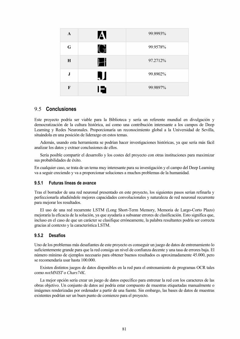
81

A

99.9993%

G

99.9578%

H

97.2712%

J

99.8902%

F

99.9897%

9.5 Conclusiones

Este proyecto podría ser viable para la Biblioteca y sería un referente mundial en divulgación y

democratización de la cultura histórica, así como una contribución interesante a los campos de Deep

Learning y Redes Neuronales. Proporcionaría un reconocimiento global a la Universidad de Sevilla,

situándola en una posición de liderazgo en estos temas.

Además, usando esta herramienta se podrían hacer investigaciones históricas, ya que sería más fácil

analizar los datos y extraer conclusiones de ellos.

Sería posible compartir el desarrollo y los costes del proyecto con otras instituciones para maximizar

sus probabilidades de éxito.

En cualquier caso, se trata de un tema muy interesante para su investigación y el campo del Deep Learning

va a seguir creciendo y va a proporcionar soluciones a muchos problemas de la humanidad.

9.5.1 Futuras líneas de avance

Tras el borrador de una red neuronal presentado en este proyecto, los siguientes pasos serían refinarla y

perfeccionarla añadiéndole mejores capacidades convolucionales y naturaleza de red neuronal recurrente

para mejorar los resultados.

El uso de una red recurrente LSTM (Long Short-Term Memory, Memoria de Largo-Corto Plazo)

mejoraría la eficacia de la solución, ya que ayudaría a subsanar errores de clasificación. Esto significa que,

incluso en el caso de que un carácter se clasifique erróneamente, la palabra resultantes podría ser correcta

gracias al contexto y la característica LSTM.

9.5.2 Desafíos

Uno de los problemas más desafiantes de este proyecto es conseguir un juego de datos de entrenamiento lo

suficientemente grande para que la red consiga un nivel de confianza decente y una tasa de errores baja. El

número mínimo de ejemplos necesario para obtener buenos resultados es aproximadamente 45.000, pero

se recomendaría usar hasta 100.000.

Existen distintos juegos de datos disponibles en la red para el entrenamiento de programas OCR tales

como notMNIST o Chars74K.

La mejor opción sería crear un juego de datos específico para entrenar la red con los caracteres de las

obras objetivo. Un conjunto de datos así podría estar compuesto de muestras etiquetadas manualmente o

imágenes renderizadas por ordenador a partir de una fuente. Sin embargo, las bases de datos de muestras

existentes podrían ser un buen punto de comienzo para el proyecto.

REFERENCES

[1] E. Peñalver Gómez, "Library of the University of Seville website," Biblioteca de la

Universidad de Sevilla, [Online]. Available:

http://bib.us.es/bibliotecas_y_horarios/machado/fondo_antiguo/fondos. [Accessed 19th

August 2016].

[2] K. A. Kluever, "Introduction to Artificial Intelligence OCR using Artificial Neural

Networks," Rochester Institute of Technology, Rochester, NY, 2008.

[3] M. A. Nielsen, Neural Networks and Deep Learning, Determination Press, 2015.

[4] Adobe, "Adobe Document Cloud - Adobe Acrobat DC," [Online]. Available:

https://acrobat.adobe.com/us/en/acrobat/how-to/ocr-software-convert-pdf-to-text.html.

[Accessed 19th August 2016].

[5] "ABBYY FineReader 12 Professional Overview," ABBYY, 2016. [Online]. Available:

https://www.abbyy.com/finereader/professional/. [Accessed 19th August 2016].

[6] "Asprise," 2016. [Online]. Available: http://asprise.com/ocr-document-scanning-

java.net/library-api-about.html. [Accessed 19th August 2016].

[7] J. Markoff, "New York Times newspaper library," New York Times, 17th August 1988.

[Online]. Available: http://www.nytimes.com/1988/08/17/business/business-technology-

now-pc-s-that-read-a-page-and-store-it.html. [Accessed 19th August 2016].

[8] L. Vincent, "Google Code Blog," 30th August 2006. [Online]. Available:

https://googlecode.blogspot.com/2006/08/announcing-tesseract-ocr.html. [Accessed 19th

August 2016].

[9] N. Willis, "Linux.com - News for the Open Source Professional," The Linux Foundation,

28th September 2006. [Online]. Available: https://www.linux.com/news/googles-tesseract-

ocr-engine-quantum-leap-forward. [Accessed 19th August 2016].

[10] Ubuntu Community, "Ubuntu Documentation," Canonical, 31st March 2015. [Online].

Available: https://help.ubuntu.com/community/OCR. [Accessed 19th August 2016].

[11] J. Schulenburg, "GOCR Project website at Source Forge," 2nd December 2000. [Online].

Available: http://jocr.sourceforge.net/. [Accessed 19th August 2016].

[12] "Ocrad page at the GNU Project website," Free Software Foundation, Inc., 26th January

2016. [Online]. Available: https://www.gnu.org/software/ocrad/. [Accessed 19th August

2016].

[13] T. Breuel, "Google Developers Blog," Google Developers, 9th April 2007. [Online].

Available: https://developers.googleblog.com/2007/04/announcing-ocropus-open-source-

ocr.html. [Accessed 19th August 2016].

84

[14] R. Smith, The Extraction and Recognition of Text, Bristol: University of Bristol, 1987.

[15] S. Rice, F. Jenkins and T. Nartker, The Fourth Annual Test of OCR Accuracy, Technical

Report 95-03, Las Vegas: Information Science Research Institute, University of Nevada,

1995.

[16] "Tesseract Open Source OCR Engine repository," 5th August 2016. [Online]. Available:

https://github.com/tesseract-ocr/. [Accessed 10th August 2016].

[17] R. Smith, "An Overview of the Tesseract OCR Engine," in Proceedings of the International

Conference on Document Analysis and Recognition, ICDAR, Curitiba, Brazil, IEEE

Computer Society, 2007, pp. 629-633.

[18] R. Smith, in 10th International Conference on Document Analysis and Recognition,

Barcelona, 2009.

[19] H. A. Song and S.-Y. Lee, "Hierarchical Representation Using NMF," in Neural Information

Processing (20th International Conference, ICONIP 2013), Daegu, Korea, Springer Berlin

Heidelberg, 2013, pp. 466-473.

[20] V. Nair and G. E. Hinton, "Rectified linear units improve restricted boltzmann machines,"

in Proceedings of the 27th International Conference on Machine Learning (ICML-10),

Toronto, Department of Computer Science, University of Toronto, 2010, pp. 807-814.

[21] G. E. Hinton, "Learning multiple layers of representation," Department of Computer

Science, University of Toronto, Toronto, 2007.

[22] Y. LeCun, "Deep Learning and the Future of AI," CERN, Zurich, 2016.

[23] J. Torres, First Contact with TensorFlow, Barcelona: Ed. Undertile, 2016.

[24] C. M. Bishop, Pattern Recognition and Machine Learning, New York: Springer, 2006.

[25] A. R. A. T. Mehryar Mohri, Foundations of machine learning, Cambridge, MA: MIT Press,

2012.

[26] R. Collobert and J. Weston, "A unified architecture for natural language processing: deep

neural networks with multitask learning," in ICML '08 Proceedings of the 25th international

conference on Machine learning, New York, ACM, 2008, pp. 160-167.

[27] S. Hochreiter and J. Schmidhuber, "Long Short-Term Memory," Neural Computation, vol.

8, no. 9, pp. 1735-1780, 15th November 1997.

[28] H. Sak, A. Senior, K. Rao and F. Beaufays, "Fast and Accurate Recurrent Neural Network

Acoustic Models for Speech Recognition," 2015.

[29] G. Cybenko, "Approximation by superpositions of a sigmoidal function," Mathematics of

Control, Signals and Systems, vol. 2, no. 4, p. 303–314, 1989.

[30] K. Hornik, M. Stinchcombe and H. White, "Multilayer feedforward networks are universal

approximators," Neural Networks, vol. 2, no. 5, p. 359–366, 1989.

85

[31] S. Nissen, "Implementation of a Fast Artificial Neural Network Library (fann)," Department

of Computer Science, University of Copenhagen (DIKU), Copenhagen, 2003.

[32] S. Nissen, Large Scale Reinforcement Learning using Q-SARSA(λ) and Cascading Neural

Networks, Denmark: Department of Computer Science, University of Copenhagen, 2007.

[33] S. Nissen, "Fast Artificial Neural Network Library," [Online]. Available:

http://leenissen.dk/fann/wp/. [Accessed 24th August 2016].

[34] LISA lab., "Theano Documentation," LISA lab., 17th August 2016. [Online]. Available:

http://deeplearning.net/software/theano/. [Accessed 24th August 2016].

[35] The Theano Development Team, "Theano: A Python framework for fast computation of

mathematical expressions," 9th May 2016. [Online]. Available:

https://arxiv.org/pdf/1605.02688.pdf. [Accessed 24th August 2016].

[36] "OpenNN - Open Neural Networks Library," 2016. [Online]. Available:

http://www.opennn.net/. [Accessed 24th August 2016].

[37] C. K. a. S. Ronan, "A Scientific Computing Framework for Luajit," [Online]. Available:

http://torch.ch/. [Accessed 24th August 2016].

[38] Berkeley Vision and Learning Center, "Caffe - Deep learning framework by the BVLC,"

[Online]. Available: http://caffe.berkeleyvision.org/. [Accessed 24th August 2016].

[39] R. M. Jeff Dean, "Google Research Blog," 9th November 2015. [Online]. Available:

https://research.googleblog.com/2015/11/tensorflow-googles-latest-machine_9.html.

[Accessed 24th August 2016].

[40] Google, "TensorFlow — an Open Source Software Library for Machine Intelligence," 8th

August 2016. [Online]. Available: https://www.tensorflow.org/. [Accessed 24th August

2016].

[41] Google Research, TensorFlow: Large-Scale Machine Learning on Heterogeneous

Distributed Systems, 2015.

[42] A. Rajavelu, M. Musavi and M. Shirvaikar, "A neural network approach to character

recognition," in Neural Networks (Volume 2, Issue 5), Elsevier Ltd., 1989, p. 387–393.

[43] C. J. J. Herault, "Space or time adaptive signal processing by neural network models," in AIP

Conference Proceedings, 151, 206-211, Snowbird, UT, USA, 1986.

[44] T. F. Pawlicki, D.-S. Lee, J. J. Hull and S. N. Srihari, "Neural network models and their

application to handwritten digit recognition," in IEEE International Conference on Neural

Networks, San Diego, CA, USA, 1988.

[45] W. P. Warren S. McCulloch, "A logical calculus of the ideas immanent in nervous activity,"

in The bulletin of mathematical biophysics, Chicago, The University of Chicago Press, 1943,

p. 115–133.

[46] U. Springmann, D. Najock, H. Morgenroth, H. Schmid, A. Gotscharek and F. Fink, "OCR

86

of historical printings of latin texts: Problems, prospects, progress.," ACM International

Conference Proceeding Series, pp. 71-75, 2014.

[47] Y. Bengio, A. Courville and P. Vincent, "Representation Learning: A Review and New

Perspectives," in IEEE Transactions on Pattern Analysis and Machine Intelligence, vol. 35,

IEEE, 2013, pp. 1798-1828.

[48] L. Deng and D. Yu, Deep Learning: Methods and Applications, Redmond, WA: NOW

Publishers, 2014.

[49] D. Cireşan, U. Meier and J. Schmidhuber, "Multi-column Deep Neural Networks for Image

Classification," IDSIA / USI-SUPSI, Manno (Switzerland), 2012.

[50] Y. LeCun, C. Cortes and C. J. Burges, "The MNIST Database of handwritten digits,"

[Online]. Available: http://yann.lecun.com/exdb/mnist/. [Accessed 30th August 2016].

[51] J. e. a. Garofolo, "TIMIT Acoustic-Phonetic Continuous Speech Corpus," Philadelphia:

Linguistic Data Consortium, Philadelphia, 1993.

[52] S. V. Rice and T. A. Nartker, "The ISRI Analytic Tools for OCR Evaluation," University of

Nevada, Las Vegas, 1996.

[53] "Elastic," Elasticsearch BV, 2016. [Online]. Available: https://www.elastic.co/. [Accessed

31st August 2016].

[54] "TensorFlow Documentation: Distributed TensorFlow," [Online]. Available:

https://www.tensorflow.org/versions/r0.10/how_tos/distributed/index.html. [Accessed 11th

September 2016].

[55] D. Barranco Alfonso and J. Bocanegra Linares, "Repositorio de GoChar - Memoria," 26th

April 2016. [Online]. Available:

https://github.com/Boca13/GoChar/blob/master/Memoria.pdf. [Accessed 5th September

2016].

[56] Google, "The Go Programming Language," [Online]. Available: https://golang.org/doc/.

[Accessed 5th September 2016].

[57] D. Barranco Alfonso and J. Bocanegra Linares, "GoChar Repository at Github," 3rd May

2016. [Online]. Available: https://github.com/Boca13/GoChar. [Accessed 5th September

2016].

[58] A. Chakraborty, "Udacity Deep Learning course - UD730," Udacity, [Online]. Available:

https://www.udacity.com/course/deep-learning--ud730. [Accessed 5th September 2016].

[59] Y. Bulatov, "Machine Learning, etc," 8th September 2011. [Online]. Available:

https://yaroslavvb.blogspot.com.es/2011/09/notmnist-dataset.html. [Accessed 9th

September 2016].

[60] Y. Bulatov, "Yaroslavvb," 2011. [Online]. Available:

http://yaroslavvb.com/upload/notMNIST/. [Accessed 9th September 2016].

87

[61] T. E. de Campos, R. B. Bodla and M. Varma, "Character recognition in natural images," in

Proceedings of the International Conference on Computer Vision Theory and Applications

(VISAPP), Lisbon, 2009.

[62] T. E. de Campos, R. B. Bodla and M. Varma, "The Chars74K dataset," University of Surrey,

15th October 2012. [Online]. Available:

http://www.ee.surrey.ac.uk/CVSSP/demos/chars74k/. [Accessed 9th September 2016].

[63] Tesseract Comunity, "Tesseract repository in GitHub," 12th 2 2016. [Online]. Available:

https://github.com/tesseract-ocr/tesseract/. [Accessed 18th 2 2016].

[64] Tesseract Community, "Training Tesseract - Tesseract Github Repository," 12th February

2016. [Online]. Available: https://github.com/tesseract-

ocr/tesseract/wiki/TrainingTesseract. [Accessed 18th February 2016].

trabajo de fin de grado -...

Documents