TR-ol-4k&

Office of Naval Research c

Contract N00014 -67-A-0298 -0006 NR-372-012 o# 9/

<7

STUDIES OF HUMAN LOCOMOTION

VIA OPTIMAL PROGRAMMING

APOllfgOS

By

C. K. Chow and D. H. Jacosson

October 1970

Technical Report No. 617

\ CO CM O T— o

.L^ lO o

, o> > o

o CM

This document has been approved for public release and sale; its distribution is unlimited. Reproduction in whole or in part is permitted by the U. S. Government.

Division of Engineering and Applied Physics Harvard University • Cambridge, Massachusetts

|f\u-ollM8<^

Office of Naval Research

Contract N00014-67-A-0298-0006

NR-372-012

STUDIES OF HUMAN LOCOMOTION VIA OPTIMAL PROGRAMMING

By

C. K. Chow and D. H. Jacobson

Technical Report No. 617

This document has been approved for public release and sale; its distribution is unlimited. Reproduction in whole or in part is permitted by the U. S. Government.

October 1970

The research reported in this document was made possible through support extended the Division of Engineering and Applied Physics, Harvard University by the U. S. Army Research Office, the U. S. Air Force Office of Scientific Research and the U. S. Office of Naval Research under the Joint Services Electronics Program by Contracts N00014-67-A-0298-0006, 0005, and 0008.

Division of Engineering and Applied Physics

Harvard University " Cambridge, Massachusetts

STUDIES OF HUMAN LOCOMOTION VIA OPTIMAL PROGRAMMING '

By

C K. Chow and D. H. Jacobson

Division of Engineering and Applied Physics

Harvard University Cambridge, Massachusetts

ABSTRACT

Research to-date towards an understanding of human biped

locomotion has been primarily experimental in nature, largely due to

the complexity of the process. In view of the new, exciting possibilities

of programmed electro-stimulation of paralyzed extremities to restore

locomotion, a critical study at the theoretical level is greatly warranted.

Optimal programming and modern control theory offer a new approach

to the study. First, it is proposed that normal walking obeys a

certain "principle of optimality". Next, at the dynamic level, modern

control theory is used to derive the optimal moment profiles which

actuate the locomotor elements to synthesize the observed patterns of

the normal gait.

Development of the problem structure relies closely on the func-

tional characteristics of the biped gait, particularly the ideas of distinct

phasic activities and the associated temporal patterns of a walking cycle.

The result is a multi-arc programming problem with three stages.

Each stage involves dynamic constraints which reflect the particular

nature of the phasic activity. Activity in the stance phase is described

{ This work is partially supported by the Joint Services Electronics Program under Contract No. N00014-67-A-0298-0006.

11

by equality constraints on the "states" while the swing phase is charac-

terized by inequality state constraints. A novelty of the approach is

that the theory could be used to study walking behavior under different

environmental conditions, such as walking up-stairs or over a hole.

Joining of the arcs is arranged in such a way as to maintain continuity

of certain trajectories as well as repeatability of motion.

A distinct feature of the present approach which differs from

other studies is the presence of a minimizing performance criterion.

Based on external characteristics of muscles and certain assumptions

regarding normal locomotion, a simple quadratic type of performance

index is proposed. This performance criterion is meaningful in that it

is shown to be proportional to the mechanical work done during normal

walking.

Invoking the necessary conditions of optimal control theory, a

multi-point boundary value problem is obtained. A penalty function

technique is then employed for iterative numerical solution on a

digital computer. Using the parameters available in the literature,

simulation results are obtained which agree well with the experimental

studies performed by Eberhart and his associates. Furthermore,

certain refined features are obtained which are not available in

previous studies. Success in applying optimal programming techniques

to human locomotion could yield better design procedures for prostheses

and could allow eventual realization of the dream of programmed

stimulation of many paralyzed persons.

Ill

TABLE OF CONTENTS

Page

ABSTRACT i

LIST OF FIGURES vii

A. PRELIMINARY CONSIDERATIONS 1

1 . Motivation 1

2. Qualitative Properties of the Biped Gait 2

a. Physiological Factors

b. The Compass Gait

c. Phasic Activities and Temporal Patterns

d. Postural Control and Stability

e. A Hierarchical Control System for Biped Locomotion

3. Energy Expenditure and "Optimality" in Locomotion 10

4. The Optimal Programming Approach 11

B. MATHEMATICAL MODELLING OF THE BIPED GAIT 13

1. Introduction 13

2. Development of the Mathematical Model 14

a. Two Basic Configurations

b. Derivation of the Model

c. Decoupling and Simplification of the Model

d. Comments

e. Kinematic Constraints

f. Quasi-Static Estimation of Ankle Moment and Reactions

IV

PaKe

3. Discussions 35

C. ON AN ENERGY PERFORMANCE CRITERION IN HUMAN LOCOMOTION 39

1. Introduction 39

2. Development of the Criterion 40

a. Assumptions

b. Derivation

i. Discussions 50

D. OPTIMIZATION IN BIPED LOCOMOTION 53

1. Problem Formulation 53

a. Dynamic Equations

b. Kinematic Constraints

c. Initial and Terminal Conditions

2. Characteristics of the Problem Formulation 55

3. Necessary Conditions of Optimality; Method of Solution 57

E. NUMERICAL SIMULATION AND RESULTS 67

1. Parameters and Pertinent Data 67

a. Physical Parameters

b. Initial and Terminal Conditions

c. Prescribed Trajectories

d. Pressure Transfer Curve

2. Numerical Computations 71

3. Results and Discussions 72

a. Angular Displacements and Related Results

b. Reaction Forces and Moments at the Joints

c. "Quality" of Numerical Computation

Page_

d. Equivalence of Kinematic and Dynamic Optimality

e. Feasible Initial and Terminal Regions

f. Design Considerations

GRAPHS #1 through #21 8 7

F. CONCLUSIONS 109

REFERENCES 111

VI1

LIST OF FIGURES

Page Fig. 1 Skeletal Muscle and Neural Pathways 3

Fig. 2 Block Diagram for Neural-Muscular Control Action 3

Fig. 3 The Compass Gait 6

Fig. 4 Temporal Patterns of Biped Gait 6

Fig. 5 Hierarchy Structure for the Locomotion Control System 9

Fig. 6 Two Basic Configurations of Biped Gait 16

Fig. 7 Ground Reaction Profiles (from Inman [31]) 16

Fig. 8 Coordinate System for the Human Locomotor System 18 Model

Fig. 9 Kinematic Constraints in Deploy and Swing Portions 30

Fig. 10 Kinematic Constraints in Stance Portion 30

Fig. 11 Typical Profiles for Ankle Coordinates in Stance Portion (from Bresler and Frankel) 34

Fig. 12 Free Body Diagram of the Foot 34

Fig. 13 Flow Chart of Model Development 36

Fig. 14 Experimental Characteristics of Skeletal Muscles [36,37] 41

Fig. 15 Agonist/Antagonist Muscle System 41

Fig. 16 Velocity-Length Characteristics (from Elftman [7]) 45

Fig. 17 Characteristic Surface of a Skeletal Muscle 45

Fig. 18 Piecewise Approximation of Characteristic Surface (Houk [42], Stark [41], Galiana [33]) 49

Fig. 19 Realization of Locomotion Program Via Multi-Arc Optimal Programming 84

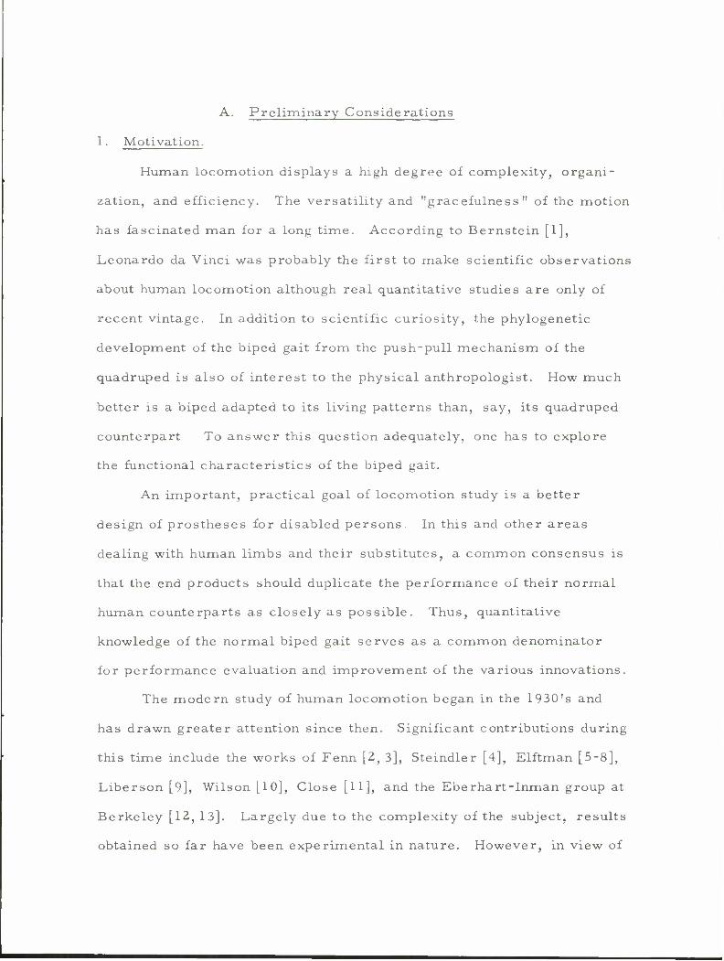
A. Preliminary Considerations

1. Motivation.

Human locomotion displays a high degree of complexity, organi-

zation, and efficiency. The versatility and "gracefulness" of the motion

has fascinated man for a long time. According to Bernstein [1],

Leonardo da Vinci was probably the first to make scientific observations

about human locomotion although real quantitative studies are only of

recent vintage. In addition to scientific curiosity, the phylogenetic

development of the biped gait from the push-pull mechanism of the

quadruped is also of interest to the physical anthropologist. How much

better is a biped adapted to its living patterns than, say, its quadruped

counterpart To answer this question adequately, one has to explore

the functional characteristics of the biped gait.

An important, practical goal of locomotion study is a better

design of prostheses for disabled persons. In this and other areas

dealing with human limbs and their substitutes, a common consensus is

that the end products should duplicate the performance of their normal

human counterparts as closely as possible. Thus, quantitative

knowledge of the normal biped gait serves as a common denominator

for performance evaluation and improvement of the various innovations.

The modern study of human locomotion began in the 1930's and

has drawn greater attention since then. Significant contributions during

this time include the works of Fenn [2, 3], Steindler [4], Elftman [5-8],

Liberson [9], Wilson [10], Close [11], and the Eberhart-Inman group at

Berkeley [12, 13]. Largely due to the complexity of the subject, results

obtained so far have been experimental in nature. However, in view of

the recent exciting possibilities of restoring the locomotion ability of

certain paralyzed limbs through programmed electro-stimulation [14-

20], a critical study of biped locomotion at the theoretical level is

greatly warranted. After all, the very fundamental question of " what

is the basic mechanism of locomotion?" or "what are the laws

governing locomotion?" cannot be answered in its completeness by

experimental study. A theory which attempts to embody the known

facts about the human gait would be an important step in this field.

Research activities to-date appear to fall into two broad areas.

The first area is concerned with the functional structure and operational

behavior of the locomotor system and its gait. The second studies

energy expenditure, oxygen consumption and metabolism in general

associated with walking. These two areas describe the important

aspects of a very complicated process. With the tools of modern

control theory, it appears possible to weld these two areas into a

"functional" theory of human locomotion. Such a study leads to quanti-

tative investigation and useful design procedures for prosthetic devices.

To this end, the relevant physiological information and gait features

are summarized. This, then, sets up the framework of our theoretical

study.

2. Quantitative Features of the Biped Gait

a. Physiological Factors [21]

Locomotion activity and other voluntary efforts usually involve

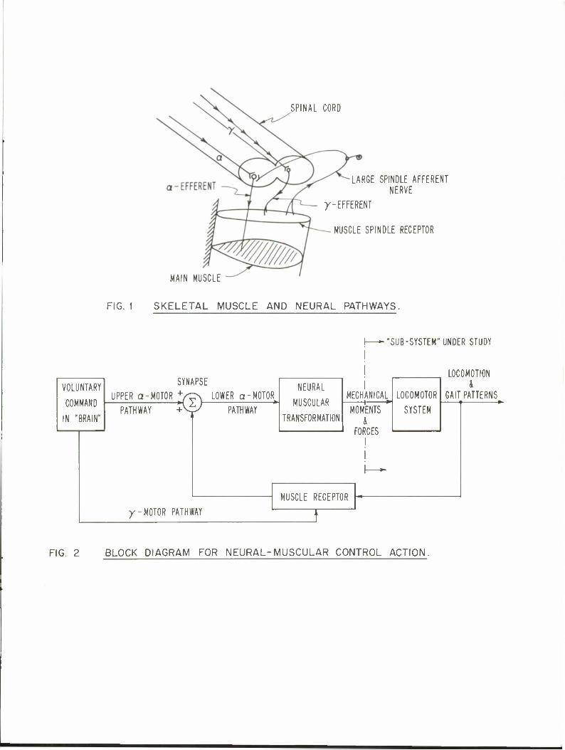
decision and supervision by the "higher centers" in the brain. Fig. 1

illustrates a typical skeletal muscle and its neural pathways. The skel-

etal muscle is the actuating unit for all locomotion activities. The

a -motor input along the spinal cord represents a direct input from the

SPINAL CORD

LARGE SPINDLE AFFERENT NERVE

/-EFFERENT

MUSCLE SPINDLE RECEPTOR

MAIN MUSCLE

FIG. 1 SKELETAL MUSCLE AND NEURAL PATHWAYS.

"SUB-SYSTEM"UNDER STUDY

VOLUNTARY

COMMAND

IN "BRAIN"

SYNAPSE R V^\ LOWER a-MOTOR

PATHWAY 4© PATHWAY

NEURAL

MUSCULAR

TRANSFORMATION

MECHANICAL + MOMENTS

& FORCES

I I

LOCOMOTOR

SYSTEM

LOCOMOTION &

GAIT PATTERNS

y- MOTOR PATHWAY

MUSCLE RECEPTOR

FIG. 2 BLOCK DIAGRAM FOR NEURAL-MUSCULAR CONTROL ACTION.

higher centers to the muscle by which the desired action can be initiated.

It is believed that the a -motor input is the signal used for voluntary

actions. A voluntary action exists in the conscious thought in terms of a

functional rather than a specific description. "Lower" in the brain, the

concept of "voluntary actions" is translated into a programmed sequence

of individual muscle actions, based on the person's experience in the

past in performing the task. The "activation" signal travels along the

a -motor pathway. A muscle spindle receptor is shown inserted in a

parallel position to the skeletal muscle. This is a transducer device

which measures the length of the muscle and its sensitivity is adjusted

by the upper y-motor neuron. Results of the measurement are fed

back to the thick lower a -motor neuron at the synapse where further

integration of activity is taken. Thus the upper a -motor neuron as

well as the peripheral sensory neuron of the muscle receptor control

the lower a -motor neuron and subsequent muscular activity.

The simple picture of neural muscular action can be shown

functionally in a block diagram in Fig. 2. The present study is pri-

marily concerned with the various mechanical moments which actuate

the locomotor system and the resulting gait patterns it produces. By

knowing the moment histories, one can then concentrate on the neural-

muscular transformation (E.M.G. activity and the like) for the

electrical patterns of activity and eventually the neural action. This

amounts to working outwards from the inner-most loop rather than

studying the entire system in aggregate.

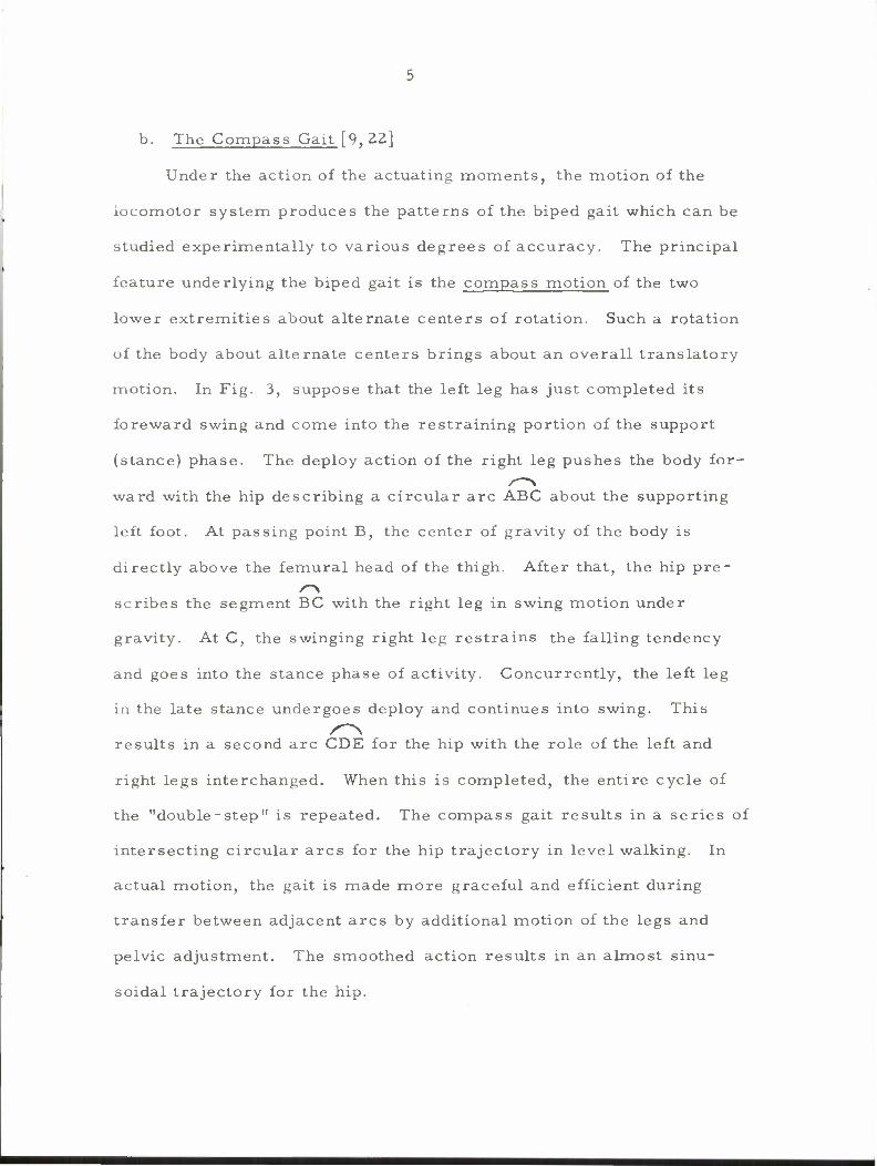
b. The Compass Gait [9, 22]

Under the action of the actuating moments, the motion of the

iocomotor system produces the patterns of the biped gait which can be

studied experimentally to various degrees of accuracy. The principal

feature underlying the biped gait is the compass motion of the two

lower extremities about alternate centers of rotation. Such a rotation

of the body about alternate centers brings about an overall translatory

motion. In Fig. 3, suppose that the left leg has just completed its

foreward swing and come into the restraining portion of the support

(stance) phase. The deploy action of the right leg pushes the body for-

ward with the hip describing a circular arc ABC about the supporting

left foot. At passing point B, the center of gravity of the body is

directly above the femural head of the thigh. After that, the hip pre-

scribes the segment BC with the right leg in swing motion under

gravity. At C, the swinging right leg restrains the falling tendency

and goes into the stance phase of activity. Concurrently, the left leg

in the late stance undergoes deploy and continues into swing. This

results in a second arc CDE for the hip with the role of the left and

right legs interchanged. When this is completed, the entire cycle of

the "double-step" is repeated. The compass gait results in a series of

intersecting circular arcs for the hip trajectory in level walking. In

actual motion, the gait is made more graceful and efficient during

transfer between adjacent arcs by additional motion of the legs and

pelvic adjustment. The smoothed action results in an almost sinu-

soidal trajectory for the hip.

STEP

FIG. 3 THE COMPASS GAIT.

-*" LEFT LEG

•- RIGHT LEG

RIGHT LEG :

LEFT LEG :

a b

^"SWING ^ C d a

STANCE DOUBLE SUPPORT

-REST RAINT^I—PROPUl SIVE-

SWING SUPPORT

FIG. 4 TEMPORAL PATTERNS OF BIPED GAIT.

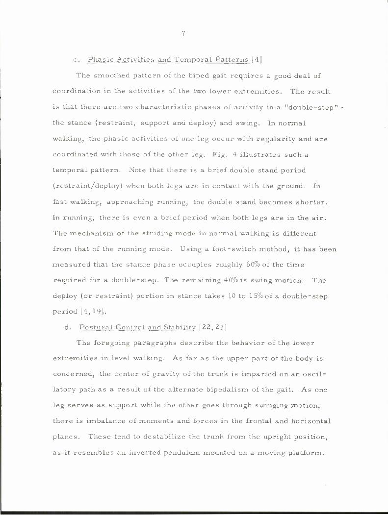
c. Phasic Activities and Temporal Patterns [4]

The smoothed pattern of the biped gait requires a good deal of

coordination in the activities of the two lower extremities. The result

is that there are two characteristic phases of activity in a "double-step"

the stance (restraint, support and deploy) and swing. In normal

walking, the phasic activities of one leg occur with regularity and are

coordinated with those of the other leg. Fig. 4 illustrates such a

temporal pattern. Note that there is a brief double stand period

(restraint/deploy) when both legs are in contact with the ground. In

fast walking, approaching running, the double stand becomes shorter.

In running, there is even a brief period when both legs are in the air.

The mechanism of the striding mode in normal walking is different

from that of the running mode. Using a foot-switch method, it has been

measured that the stance phase occupies roughly 60% of the time

required for a double-step. The remaining 40% is swing motion. The

deploy (or restraint) portion in stance takes 10 to 1 5% of a double-step

period [4, 19].

d. Postural Control and Stability [22, 23]

The foregoing paragraphs describe the behavior of the lower

extremities in level walking. As far as the upper part of the body is

concerned, the center of gravity of the trunk is imparted on an oscil-

latory path as a result of the alternate bipedalism of the gait. As one

leg serves as support while the other goes through swinging motion,

there is imbalance of moments and forces in the frontal and horizontal

planes. These tend to destabilize the trunk from the upright position,

as it resembles an inverted pendulum mounted on a moving platform.

8

To maintain upright position and minimize undesirable oscillations,

coordination of various muscle activity is needed. From a locomotion

standpoint, the progressive translation of the body is of main concern.

The associated unstable tendency of the trunk is an unfortunate conse-

quence inherent in the biped gait.

e. A Hierarchical Control System for Biped Locomotion

From the temporal, phasic and stability properties of the biped

gait, it is quite apparent that the locomotion process is involved indeed.

It has been postulated that the control system possesses a hierarchical

structure, with two or more levels of decision, coordination and

regulation for a desired gait and adaptation within a given environment.

Important objectives of the control system would be:

(1) determination of speed, step length parameters and direction

of progression

(2) synchronization of the motion of the two extremities to

achieve coordinated phasic activities and temporal patterns

(3) adaptation to ground profile within a double-step

(4) maintenance of up-right posture .

With the exception of (1), the gait features we have described

fit into the objectives of the controller. From an organizational view-

point, the goals (3) and (4) are realized by a control system under the

supervision of a higher level controller connected to (1) and (2). A

schematic diagram of the locomotion system would appear as shown in

Fig. 5.

Such a functional structure for the control system possesses the

advantages described by Tomovic [24]:

DECISION ORIENTED

LEVEL n

ALGORITHMIC OR

HIGHEST LEVEL: CONSCIOUS

DECISION MAKER

AUTOMATON LEVEL II

DYNAMIC LEVEL

INFORMATION FEEDBACK

'e.g. VISUAL, MECHANICAL,PAIN, ETC.

2ND LEVEL: SYNCHRONIZATION

OF MUSCLE GROUP

ACTIVITIES AND PARAMETER

DETERMINATION

INFORMATION FEEDBACK

CONTROLLER V

V

L^_ OPTIMAL PROGRAMMING

& ADAPTATION

FOR A

PARTICULAR

MOVEMENT

L.^X

2

'FEEDBACK" INTERACTION BETWEEN

SUBCONTROLLERS

1

"FEEDBACK @ VARIOUS LEVELS

FIG. 5 HIERARCHY STRUCTURE FOR THE LOCOMOTION CONTROL SYSTEM

10

(1) A minimal amount of supervision required on the part of

controllers at the algorithmic and higher levels in executing well-

learned tasks such as normal level walking.

(2) Flexibility at the dynamic level to adapt to a particular

environment witnin a double-step.

The present interest is in finding out the various actuating

moments to simulate the biped gait. This implies that the analysis is

performed at the dynamic level of the hierarchical system. The choice

of speed of walking, step-length, direction and other relevant parameters

are the goals of the algorithmic controller, as is the coordination of

muscle group activities.

3. Energy Expenditure and "Optimality" in Locomotion

Besides the broad study of the functional characteristics of the

biped gait, the ergonomics of locomotion forms another important area

of research. An average person walks over a million steps in a year

and certainly many times more over the span of his lifetime. In situations

such as level walking where speed is not an important factor, it is thus

very appealing to think that the walking activity would involve minimiza-

tion (optimization) of some type of energy performance criterion. In

search for such an "optimality" in locomotion, experimental studies in

energy expenditure, oxygen consumption associated with locomotion have

been performed. Significant contributions include the works of Fenn,

Elftman [7], Ralston [25], Cotes and Meade [26]. Earlier results were

obtained by Atzler and Herbst. Theoretical attempts to formulate or

demonstrate a "minimal" principle were made by Nubar and Contini [27]

and Beckett and Chang [28].

11

By far the most interesting result has been the measurement of

mechanical work done by the various body members during walking as

a function of speed, step-length and pace frequency parameters. In

the experiments by Atzler and Herbst as reported in Elftman [5], they

plotted energy expenditure for different speeds and step lengths. A

minimum expenditure curve exists for the appropriate combinations of

speed and step-length. In a more recent study by Coates and Meade,

similar results were obtained and various expressions were obtained

from experimental data by interpolation. Milner [20] and his associates

performed quantitative study of EMG activity of the muscles of the

lower extremities in connection with the programmed electro-

stimulation problem. In particular, they showed that the EMG activity

is minimum when their human subject is allowed to walk at a pace

frequency of his own choice for a given speed of walking. Whether

human locomotion does indeed obey an optimality principle has not

been proved by experiment or theory, but the results gathered to-date

do support the suggestion.

4. The Optimal Programming Approach

We have briefly summarized the two important areas of loco-

motion research. To cast the biped gait in an optimization context,

the underlying hypothesis is that the locomotion activity follows a

principle of optimality. In the subsequent analysis, an appropriate

minimizing performance criterion is developed which reflects or

measures the mechanical work done by the muscles of the lower extrem-

ities during walking. The system dynamics and auxiliary constraints

will be developed on the basis of gait information mentioned earlier.

iZ

Numerical solution of the resulting optimization problem leads to

specification of the various moment quantities and the simulation of

gait patterns on the basis of minimum mechanical energy expenditure.

This approach, using modern control theory, attempts to unite

the two areas of experimental work. It differs from the other studies

in that the actuating moments are not predetermined on experimental or

intuitive grounds. The programming approach, if proved fruitful,

opens a new way to study the locomotion problem and quantify prosthetic

design. To formulate the problem structure, specification is required

of the following:

(1) An appropriate mathematical model for simulating the

functional behavior of the locomotor system.

(2) Auxiliary constraints - kinematic and dynamic on the basis of

gait information.

(3) Initial, terminal and "inflight" conditions.

(4) An optimality criterion which can be extremized to yield the

actuating moments and other quantities of motion.

13

B. Mathematical Modelling of the Biped Gait

1. Introduction.

In a quantitative study of the biped gait, the important moving

units are not the various bones which support the surrounding tissues

but the total mass of the segments which rotate about their respective

joint axes. The central straight line which extends between two axes of

rotation is called a link. This may be longer or shorter than the parti-

cular bone it represents. For example, the femur and humerus are

longer than their respective links while the tibia and radius are shorter.

Functionally, the human body is an articulated system of links.

Although the overall displacement of the body is translatory, motion is

achieved by angular displacements of the links about their respective

axes. The compass motion as mentioned earlier is the basic mechanism

of biped locomotion. The objective of mathematical modelling is to

describe the angular motions and relate them to the overall translatory

process of locomotion. Such a mechanical description is separated

from the action of the muscles and other physiological considerations.

The multi-linkage models have been studied by Nubar and Contini

[27]; Vukobratovic and his associates [22, 23, 29]; Beckett and Chang

[28]; and Hill [30]. Complexity of the models developed depends on the

assumptions made about the gait and degrees of freedom allowed in the

motion. In a paper by Nubar and Contini, a system of linear differential

equations was derived for small angle dynamics. However, they set

pertinent derivatives to zero and studied only static configurations of the

gait. Marie and Vukobratovic formulated the leg in level walking as a

two link system. The assumptions on the gait were that the hip was

14

stationary and the foot in continuous contact with the ground during a

double-step. There was no mention of the reactional and internal forces.

In two joint papers by Vukobratovic, Frank and Juricic, the stability

problem of the trunk was studied on the basis of a compass gait for the

lower extremities. In the same vein, Beckett and Chang studied the

kinematics of swing phase motion under a "minimum energy" hypothesis,

but the interesting point is that they obtained the moment profiles without

any optimization procedure. Lastly, Hill proposed a nine degrees of

freedom model for postural study. The dynamic equations are

apparently too lengthy to derive.' Thus it appears that realistic efforts

in modelling are still lacking. The works done to-date share the

following features:

(a) They are multi-linkage type mechanical models.

(b) The analysis is confined to motion in the sagittal plane.

(c) Only the case of level walking has been treated. Other

configurations such as walking upstairs, downstairs, or over rough

terrain have not been considered at all.

(d) The models have been much simplified to render the problem

tractable. The result is that they embody little or none of the described

properties of the actual biped gait.

2. Development of the Mathematical Model.

The present model emerges as a compromise between complex

high order models and the simple two-link type. Under suitable

assumptions, a high order model is decoupled into two parts. The part

relevant to lower extremity is still of a two-link type. However, appro-

priate constraints are imposed to insure realistic simulation of the #ait

15

patterns. Modern control theory can handle constraints effectively

while the classical methods cannot. The development of such a

"constrained" mechanical model takes place in the following stages,

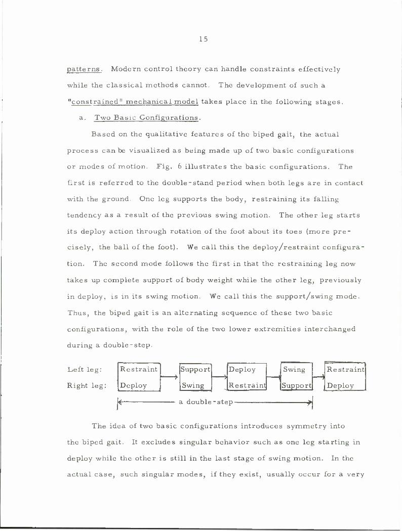
a. Two Basic Configurations.

Based on the qualitative features of the biped gait, the actual

process can be visualized as being made up of two basic configurations

or modes of motion. Fig. 6 illustrates the basic configurations. The

first is referred to the double-stand period when both legs are in contact

with the ground. One leg supports the body, restraining its falling

tendency as a result of the previous swing motion. The other leg starts

its deploy action through rotation of the foot about its toes (more pre-

cisely, the ball of the foot). We call this the deploy/restraint configura-

tion. The second mode follows the first in that the restraining leg now

takes up complete support of body weight while the other leg, previously

in deploy, is in its swing motion. We call this the support/swing mode.

Thus, the biped gait is an alternating sequence of these two basic

configurations, with the role of the two lower extremities interchanged

during a double-step.

Left leg:

Right leg:

Restraint

Deploy

1

I*

Support

Swing

Deploy

Restraint H a double-step-

Swing

Support

Restraint

Deploy

The idea of two basic configurations introduces symmetry into

the biped gait. It excludes singular behavior such as one leg starting in

deploy while the other is still in the last stage of swing motion. In the

actual case, such singular modes, if they exist, usually occur for a very

RESTRAINT / DEPLOY SUPPORT/ SWING

FIG. 6 TWO BASIC CONFIGURATIONS OF BIPED GAIT.

-0.25Wh- 100%

stance and deploy

W = Weight of body

(R) = Restraint

(S) = Support (D) = Deploy

[31] FIG. 7 GROUND REACTION PROFILES (FROM INMAN).

17

brief interval so that they can be neglected in a first study. In the

current literature, the restraint, support, and deploy portions are

collectively known as the stance phase of activity. In our formulation,

we will refer to restraint and support collectively as the "stance"

portion.

b. Derivation of the Model.

Fig. 8 depicts a high degree of freedom model for motion in the

sagittal plane. Considering the locomotor system as a whole, the

inertial and gravitational effects of the foot are small in comparison with

those of the shank or the thigh. The average weight of a foot is about

1 to 1. 5% of the body and its dimensions are also small (approximately

j ) as compared to the thigh or the shank. Furthermore, its behavior is

more or less specified in a double-step. This is so because, in the

stance position, the foot is almost stationary except for a brief moment

following heel strike to absorb impact. In deploy, the ankle of the foot

describes a circular arc with the center of rotation located about the

ball of the foot. In swing, the foot is locked withthe shank at an approxi-

mately constant angle. Such a kinematic behavior of the foot can be

described by appropriate constraints on the thigh and shank variables.

Dynamically, the foot is subjected to large ground reaction forces which

exceed body weight in the stance position. Characteristic profiles of the

forces are shown in Fig. 7. The actual "shape" of these forces depends

primarily on the gravitational and inertial effects of the motion of the

upper part of the body. The internal forces X, Y at the ankle joint in turn

depend almost entirely on the ground reactions. The up-shot of all this is

that the behavior of the foot can be alternatively described by appropriate

hip trajectory

(h(t),v(t))

V, Potential Energy =0

FIG. 8 COORDINATE SYSTEM FOR THE HUMAN LOCOMOTOR SYSTEM MODEL.

NOTATION: a, « distance of center of gravity of the thigh segment from hip joint (H) knee " (K)

ii ii it ii ii II shank II II

{, -- length of the thigh segment l2= shank "

m, £ mass of the i-th segment (i • 1 -* thigh; i • 2 => shank; i = t => HAT section)

Y,X • vertical and horizontal reactions at the ankle Ma= ankle moment

Uj= effective moment for the i-th link

L9

constraints and equivalent forces at the ankle. This device reduces the

order of the system dynamics.

With the motion of the foot considered, we are now in a position

to derive the mathematical model for the locomotor system. To

achieve symmetry in the equations, let (h(t), v(t)) denote the horizontal

and vertical position of the hip. Let the variables <j> and y De assigned

to describe the leg in the stance portion. The leg in deploy and swing

is described by the angles x, and x?. The head, upper extremities and

trunk portions are collectively considered as a single link described by

the variable w. Note that the hip position (h(t), v(t)) is a function of the

variables <ji, y. This is also dependent on x. and x_ in the deploy

portion, i. e. :

h = XA " *1 sin (^ ' K] + *2Sin (Y " ^ + K) (M

v - y» + ^i c°s (9 - <J) ) + S.? cos (y - (j> + 4 )

where (x.,y,) denote the position of the ankle. Similar expressions

hold for the x, and x . variables in the deploy portion. To carry out

the derivation by use of Lagrange's equations, expressions for the

kinetic and potential energies of the various links are needed. The

centers of gravity for the respective links are:

(1) thigh in stance portion

*4 = h+ a 1 sin (4" <j>0)

^4=v"a 1cos ^ ' (^o)

(2) shank in stance portion

x = h + i. sin (<j> - (j> ) - a _ sin (y - cj> + cji )

7 == v - lj cos (4 - 4Q) - a 2 cos (y - 4 + 4Q)

(2)

(3)

(4)

(5)

(6)

20

(3) thigh in deploy and swing portions

x, = h + a sin (x, " 4 )

y. = v ~ a , cos (x, - cj> ) 1 i 1 ' o

(4) shank in deploy and swing portions

x -> - h + St. sin (x, - d> ) - a sin (x-, - x. + <j> ) Z L 1 To 2 2 1 To

y 2 = v - t, cos (x, - q> ) - a _ cos (x? - x. +9 )

(5) trunk motion for all portions

x - h -r a sin u

y = v +• a cos u

The velocity of the center of gravity for each link is obtained through

differentiation with respect to time. From this, the total kinetic

energy of a link is the sum of translation component due to motion of

C. G. and rotation about the C. G. , i.e.:

(T) = (T + T ) v 'i-th link v C.G. Rot. 'i-th link. (7)

The total kinetic energy of the link system is

T = Ti+T+T+T+T- (8) 9 v x, X2 CJ

After manipulation, rearranging and regrouping terms, the total

kinetic energy expression can be concisely expressed as

T = j A0(^ +^) +1 V2 +| A2(v - <fr)2 +i Ajx^+I A2(k2-Xl)

2

+ i Aji + C1x1(ht2 + vtj) + C2(x2 - x^i-ht^ + vtj)

- C3Xl(x2 - Xl)t6 + C1cf(ht2 + vtj) + C2(y - i)("ht4 + vt3)

- C^<j>(y - <j>)t/ + C£-w(h cos w - v sin w) (9)

21

where A = 2(m, + m,) -t- m o I c. I

2 2 A. = I. +m.a •{• m-pi,

A2 = h +m2a2 2

A =1 + m a

C , = m , a 1 + m^f.

C2 = m2a2

C3 ^m2a2*l = CVl

C _ = m a 5 u u

tL - sin(<j> - 4Q) t1 = sin(x1 - cj> )

t., = cos(d) - (j) ) t_ = coslx. - d> ) 2 T ' o 2 1 To

t0 = sin(v _ 4 + cj) ) t_ - sin(x_, - x, + (j> ) i ' 7 7 o 3 2 1 To

t4 - cos(y - 4 + 4Q) t4 = cos(x2 - Xj T 4Q)

f

t5 = sin(y) t5 = sin(x2)

! t, - cos(y) t, = cos(x-)

Similarly, the total potential energy of the system is

~= (AQV - C1tz - C2t4 - Cjt2 - C2t4 + C5cos u) (10)

The equations of motion are obtained by substituting the T and V

expressions into

d / 9T\ dT 9V dT(aq-)-¥q7+ SqT = Mx <">

where q. represents the angular variables and M. the effective moment

for the appropriate link. The result is a system of five nonlinear,

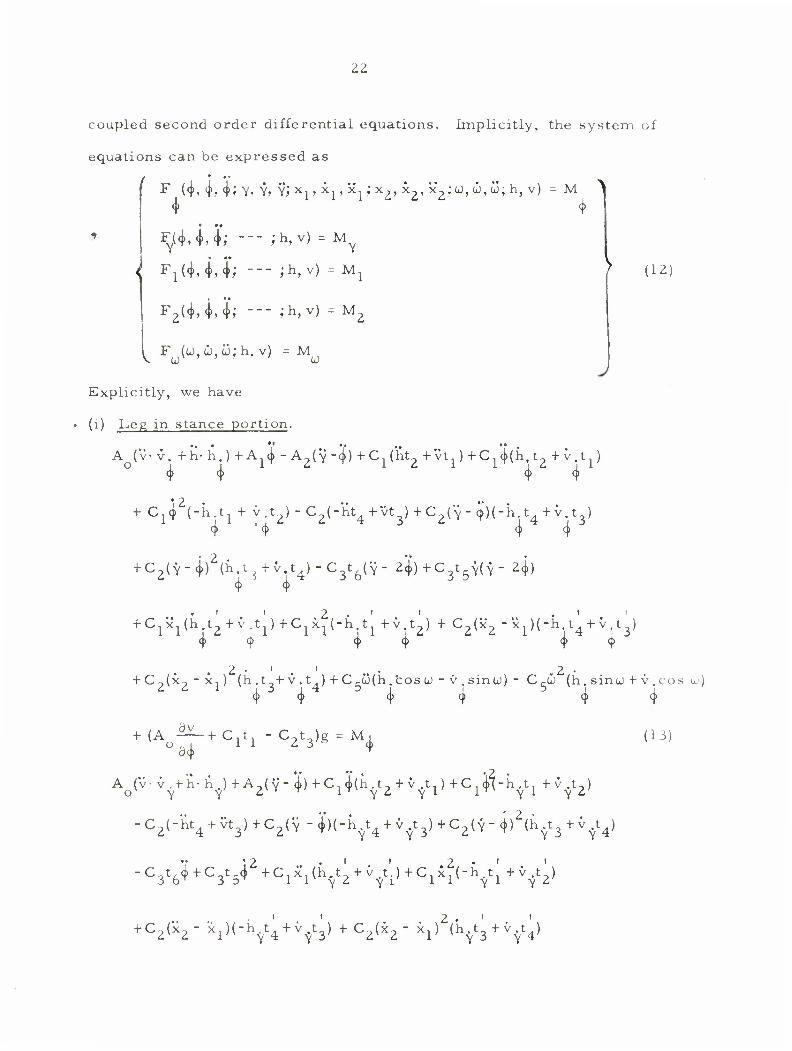
22

) (12)

coupled second order differential equations. Implicitly, the system of

equations can be expressed as

F (<h<j>>4> Y» Y> YJXxjXpX^x^j^j^jUjWjW^h, v) = M

F(4,<M; --- ;h,v) = My

^(4,4,4; --- ;h,v) -. Ml

F2<4, M; -— ;h,v) = M2

^ Fw(u,u,u;h. v) = M^

Explicitly, we have

(1) Leg in stance portion.

A (v- v. +h-h.)+A,i -A0(y-$) + C1(ht0 + vt. ) +C .'i(h, t, + v.t.' ° 4 412 1211i2<j,1

+ C1<j>2(-h.t1 + v.t2)-C2(-ht4 + vt3)+C2(Y-$)(-h.t4 + v.t3)

+ C2(-y-cj>)2(h.l3+v.t4)-C3t6(Y- 24)+C3t5y(Y- 4) 4 " 4

J

I I .2, i i t i

4-C/x, (h.t, + v.t, ) +C1x.(-h.t, + v.t„) + C0(x, - x, )(-h,t . +v.t.) 1 1 i £ .1 11 i 1 \ c. L c. 1 i4 i3

cp cp cp cp cp cp

2 • ' . ' • , 2 • + C2(x-,-x,) (h.t +v.t ) + CrC(h.bosu-v.sinu) - Cri (h.sinu + v.cos u)

cp ~ cp cp Cf cj> cj>

9v

3cp '

•« •• •• . '2 • A (v-v , + h-h .)+A-,(V-4)+C14(h.t0+v .t, )+C,4(-h.t. + v.t,)

o Y Y ^ ' T iTY2 Y 1 1 Y 1 Y ^

(13)

C2(-ht4 + vt3)+C2(Y -4)(-h.t4 + v.t3)+C2(Y-4) (h^t3+v.t4)

C3t64+C3t5ci2+C1x1(h.t2 + vtt,.)+C1x2(-h.t;+v.t2)

i i

•*lH-V4 + SV +C2<*2" ^l^V^Vi1

^3

+ <Ao-f7 + C2t3)g = MY (14)

2 where h = -rrh: h = —s- h: h. - — h and similar expressions hold for

dt (J. a<|>

v., v, v, etc. The effective moments Mi and M are given by 4 9 Y

Mi = Uj + M, + Y(l tj- t2t ) + X(£1t2 + it.) (15)

M = u0 - M + Yl0t, - Xj^t, (16) Y £ Y ^ 3 c 4

u, = Moment generated by muscle action about the hip joint

u? = Moment generated by muscle action about the knee joint

M = Ankle moment a

Y = Vertical component of the internal reaction force at the

ankle joint

X = Horizontal internal reaction at the ankle.

Specification of the quantities X, Y and M will be considered later.

(ii) Leg m deploy portion.

... ••'..' A(v-v. +h-h. )+A.x, - A_(x, - x,) + C, (ht0 + vt. ) o x, x, 11 2 2 1' 1 2 1

+ ci2i<ii1v%ti)+ci*i<"&A1ti+*i1v -c2(-ht;+vt;)

+ C2(^"'^l)("flx1t4+{rx1

t3)+C2(i2"il)2^x1t3+^x1

t4)

- Cot,-(x0 - 2x, )+Cotcx0(x0 - 2x, )+C, d>(h. t0+v. t, ) 3 6 t 1 3 5 A 2 1 1TX x, 2 x, 1

+ C1^-n.it1+v.it2)+C2(Y^')(-h^t4 + v.it3)

' 2 • . •• • + C?(Y

_4) (h- ^+v, t )+Cc;w(h. cosw-v. sin w)

^ X. J X-I * -^ X. Xi

- C u (h. sin w + v. cos u) + (A |^— + C.t - C?t )g = M. (17)

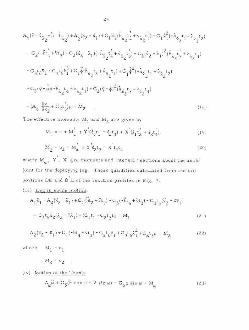
Z4

Ao<v'- vfi' V+V$2"xi)+cisi(V2+Vi>+Ci^("V^St2)

-c2(-ht;+^)+c2(xfxp(4 t;+v t;)+c2(x2-x/(h t;tv t)

fS^i'H\VV3)+C2(i"*'\t3 + ;x2t41

The effective moments M, and M? are given by

81*1 •|2t3) + X'(£lt2 1 Ml = u + Ma + Y'(Vl ' V^ + X'(jeit2 + £2t4) (19)

M =u2 -M* +Y,i-t_ -X'i,t, (20) l2 "2 a 2L3 2 4 ! 1

where M , Y , X are moments and internal reactions about the ankle

joint for the deploying leg. These quantities calculated from the tail i

portions DE and D E of the reaction profiles in Fig. 7.

(iii) Leg in swing motion.

AJJCJ -A2(x2-x1)+C1(nt2+vt1)-C2(-ht4 + vt3)-C3t6(x2-ZxI)

+ C3t5X2(x2 -2x1) + (C1t[ "C2t3)g - Ml (21)

A2(x2- 5J1)+C1(-'ht4+vt3)-C3t6x1+C3t5x^+C2t3g - M2 (22)

where M. = u.

M2 = u2 .

(iv) Motion of the Trunk.

A LJ + C,-(h cos u - v sin u) - Ccg sin u - M (Z3)

25

where

M^ = uy - Ul (24)

u = effective moment due to muscle actions of the trunk and upper extremities.

Equation groups (i) and (ii) form a system of coupled equations

describing the motion in the restraint/deploy configuration. Note that

the expressions are identical except for the interchange of variables -

x, and x? for <j> and y. This is reasonable as both legs are in contact

with the ground and the (h, v) - description for the hip position introduces

symmetry into the expressions. In state variable language, the system

of equations is equivalent to an eight-dimensional vector differential

equation. Equation groups (i) and (iii) describe the support/swing mode

of motion. The swing equations are comparatively simple and contain

no (j>, y variables explicitly. Equation (iv) describes the trunk motion in

the sagittal plane.

c. Decoupling and Simplification of the Model.

The foregoing equations describe the complete behavior in the

sagittal plane and no approximations have been introduced. Motion of

the body in the frontal and horizontal planes will introduce additional

equations but no modification in the present ones. However, such a

"high order" model is very complex to handle. Although the differential

equations can be numerically integrated as an initial value problem,

what is at hand is a multi-point boundary value problem from the optimal

programming formulation. Simplification of the model is necessary to

render the problem tractable and to obtain insight into the problem. The

major complexity of the model is in the coupling of motion between the

two lower extremities as expressed in (h, v) and their various derivatives.

26

The central idea in simplification is to decouple the motion of the two

legs. In level walking over the range of normal speeds, pace frequency

and step-length, the hip position (h, v) describes a characteristic

trajectory. The horizontal component, h, is uniform motion while the

vertical component describes a double period sinusoid about some mean

value. Thus, to obtain a realistic simulation of lower extremity motion,

one may introduce the auxiliary constraints

h = XA " ll sin((* " <U + lZ sin <Y " 4 + 40) = %-) (25)

v = yA + lj cos ((j. - 4Q) + £2 cos (y - 4 + 4Q) = "g (t) (26)

for the leg in stance and where f(t) and g(t) are prescribed time

functions for the hip trajectory. Similar expressions hold for the leg

in deploy. The auxiliary constraints simplify the equation groups (i),

(ii) and (iii) somewhat but we still have a high order model as h„, h.,

4 h. , h. , etc. are non-zero. To obtain further simplification, it is

xl x2 assumed that all the partial derivatives are zero, i. e. h. = 0, v. = 0

4 4 and so on. Such a step amounts to the consideration of the hip as the

origin of a moving coordinate system, prescribing the characteristic

trajectory of the hip. Useful expressions for the hip position are

f(t) = vQ(t + tQ) ; [ft] (27)

g(t) = eo "T2 Sin¥(t + P ' T) : [ft] (28)

where v = velocity of level walking o °

t = constant based on the initial configuration of the system

e = average height of the hip above the ground

T = period of a double-step

j3 = constant dependent on initial conditions of motion.

27

The device of prescribing a hip trajectory has been used by Galiana

[33], Beckett [28] and Wallach [34] in their various studies. From

this, we obtain a decoupled model for the optimization problem.

Simplified Dynamics.

(i) Stance Portion.

(A1 +2C3t6)i' " (A2 +C3t6)Y + C3t5Y(Y-2ci)) + (C1t1 -C^HV + g)

= ux + MQ + Y(£1t1 - i2t3) + X(i1t2 + t2t4) (29)

- (A2 + C3t6)| + A2y + C3t542 + C3t6(v + g) = uz - Ma + Y£2t3

- ^2t4X (30)

v = g (31)

(ii) Deploy and Swing Portions.

The form of the equations is identical with those of (i) except for

the following:

(a) The variables x, and x, replace cj> and y-

(b) The terms M , Y , X replace the corresponding terms

in (i) for the deploy portion.

(c) In swing, all terms due to ankle moment and reactions

vanish.

Because of the similarity in the equations, we can now adopt a

common notation. Let x, and x? stand for the thigh and shank angles

respectively (i. e. for cj> and y in stance; x, and x? in deploy and swing).

Define also x_ = x,; x. = x?, then we obtain the equations in first order

canonical form

x(t) = f(x,~;t) (32)

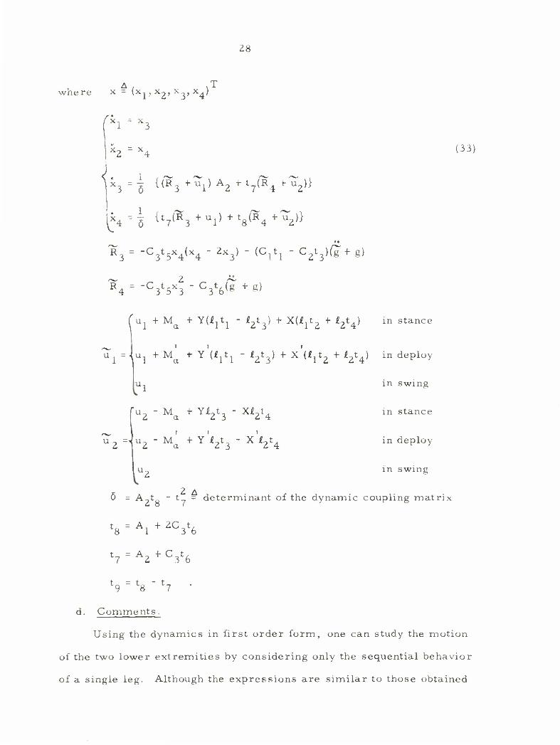
Z8

where x - (X|,x2, x^x^

Xl = X3

X2 = X4

U3=i {(R3+^1)A2+t7(R4 + u2)}

x4 - ^ {ty(R3 + Uj) + tQ(R4 + ~2)} V.

R3 = 'SV^ ' 2x3) " {C\h " C2t3)(g + g)

(33)

R4 = -C3t5x3 - C3t6(g +

u + MQ + Y(£1t1 - £2t ) + X(£1t + j?2t.) in stance

i i i

u = iul + MQ + Y (£1t1 - £2t ) + X (£jt2 + £2t ) in deploy

in swing

in stance

in deploy

in swing

6 - A,t - t - determinant of the dynamic coupling matrix

t7 = A2 + C3t6

u, - M + Y£0tQ - Xtjl. 2 a Z 3 Z 4

u. - M + Y £,t^ - X £-,t. 2 a 2 3 2 4

d. Comments.

Using the dynamics in first order form, one can study the motion

of the two lower extremities by considering only the sequential behavior

of a single leg. Although the expressions are similar to those obtained

^9

in two-link models, we have placed into perspective that the simplified

model is obtained through decoupling of a high order one. In the model

by Beckett and Chang, only the kinematic aspects of the motion are

considered by neglecting all reactions and ankle moment contributions.

Wallach's [34] paper on knee prosthetics also neglected the forces and

moment. In the paper by Galiana [33], the ankle moment term was

missing as a result of the "fixed-foot" assumption. The decoupled

equations are identical to those derived by Bresler and Frankel [13]

using the D'Alembert's principle of dynamic equilibrium for their

experimental study. Their important results indicate that the ground

reaction forces in the stance portion are the most significant quantities

and gravitational and inertial effects of the thigh and shank variables

are small compared to these. Thus it appears that the simplified model

should yield realistic results provided appropriate consideration of the

foot motion is taken.

e. Kinematic Constraints.

In the deploy portion the ankle of the foot describes a circular

arc about the ball of the foot. With the hip motion prescribed, the

angles x, and x? are no longer independent but subjected to an equality

constraint relationship. Suppose that deploy starts at time t and ends

at t?. Vertical displacement is summed to yield

eo =/8(*l> + *iCOs(x1(t"1) - 4Q) + 42cos(x2(t~) - X^t") + 4Q)

+ dsina(t, )

as shown in Fig. 9. The angles x, (t. ), x?(t. ) and a (t, ) are specified.

Similarly, for t < t "^ t , we have

e ='g(t) +£,cos(x,(t) -cj> ) +Lcos(xJt) - x,(t) + (j> )+dcos<x(t).

0 (Deploy) (Swing)

FIG. 9 KINEMATIC CONSTRAINTS IN DEPLOY AND SWING PORTIONS.

vilLh(t)= v(t*t0)

Stance portion

(0)

Shank

(q,p)= Coordinates of the ankle (primary rotation center)

FIG. 10 KINEMATIC CONSTRAINTS IN STANCE PORTION.

31

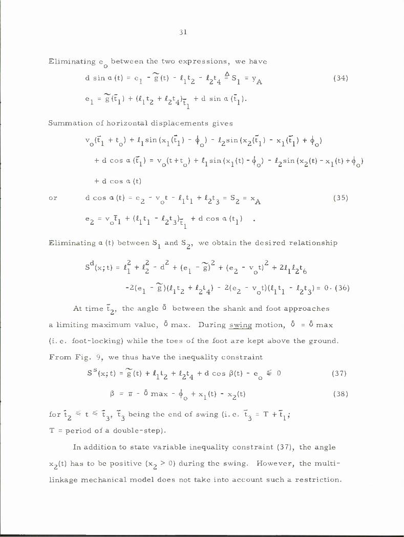
Eliminating e between the two expressions, we have

d sin a (t) = ex - ^(t) " ^2 " V4 " Sl = yA (34)

S (xjt)^ +£2-d +(Cl -g) *(e2-v t)' . .n

ej = g (tx) + (ij^ + i2t4)- + d sin a (tj).

Summation of horizontal displacements gives

Vo(Fl + to) + *isin(xl(V " 40) " ^2sin(x2(ri) - x^) + 4Q)

+ d cos a (t^ = v (t+ t ) + ^1sin(x1(t) - 4 ) " *2sin(x2(t) - x,(t) +4 )

+ d cos a (t)

or d cos a(t) = e, - v t - i.t, + £_t., = S0 - xA (35) <£ oil 23 2 A

e2 = v ^1 + ^1*1 " ^S^t + d COS a ^0

Eliminating a (t) between S, and S we obtain the desired relationship

-2(e1 - g )(lltz + i2t4) - 2(e2 - v^K*^ - i^) = 0- (36)

At time t?, the angle 6 between the shank and foot approaches

a limiting maximum value, 6 max. During swing motion, 6=6 max

(i. e. foot-locking) while the toes of the foot are kept above the ground.

From Fig. 9, we thus have the inequality constraint

SS(x;t) ="g(t) + ljt2 4- l£ + d cos p(t) - e $0 (37)

(3 = 77 - 6 max - 4 + x,(t) - x2(t) (38)

for t? ^ t ^ t , t being the end of swing (i. e. t = T + t •

T = period of a double-step).

In addition to state variable inequality constraint (37), the angle

x?(t) has to be positive (x2 > 0) during the swing. However, the multi-

linkage mechanical model does not take into account such a restriction.

u

This aspect of model limitation does not appear to have been noticed in

previous investigations. A useful device to alleviate the difficulty is to

adjoin a "soft" penalty [35] to the performance criterion J under optimi-

zation', i.e. define

/> dt

for a sequence of y : y >Yi>Yo >Y —*"^J_- The penalty becomes

effective as x?—»0 but smaller as x?(t) becomes more positive. A

restriction is that in iterative computation, the trajectory x?(t) has to

remain feasible, i.e. x?(t) > 0 Vt e [t?,t ]. Intuitively, the factor

Ys —7-. is equivalent to a nonlinear spring placed about the knee joint and X-p \T.)

the parameter y measures its stiffness.

In the stance portion, the foot is more or less stationary except

for the brief moment following heel strike. The dynamic behavior is

difficult to describe because a rigid link cannot describe the behavior of

a "round" foot. Fig. 10 illustrates the roll-over situation where the i

weight bearing leg rotates about its ankle (0 ) - the primary rotation

center. The pressure center where the ground reaction forces are

acting is gradually transferred from the heel towards the toe. The

effective kinematic constraints in this period are that the ankle (x.,y.)

coordinates follow a prescribed trajectory, (q(t),p(t)). In a rough

analysis, q(t) and p(t) can be taken as constant. Thus, we have

S^S(x;t) =^(t) + iYtz + L,t4 - eQ + p(t) = 0 (40)

S"(x;t) = VQ(t + tQ) + ^tj " y3 " q(t) =0 (41)

j J has yet to be defined.

33

The particular choice of p and q profiles has to depend on experimental

data. Fig. 11 shows the typical profiles. Note that they are almost

constant except for the initial restraining moment.

f. Quasi-Static Estimation of Ankle Moment and Reactions.

Having developed the dynamic equations and kinematic constraints,

the model is incomplete until the ankle moments and reaction forces

are known. Fig. 12 shows a free body diagram of the foot. The forces

f and f represent the vertical and horizontal components of the ground

reactions due to weight bearing and trunk motion. These forces have

been measured by various investigators using force plates and Fig. 7

shows the typical, normalized profiles over a wide range of level walking

speeds and step-lengths. To describe the foot motion, we write the

equations for translation motion for the center of gravity (O^.,) and

rotation about 0„. On summing the vertical forces, we have

*VF = fv " MFS " Y

or Y = fv - MFg - (MFyF) . (42)

Similarly, summing the horizontal forces gives

F F h

or X = f, - M "x- . (43) h F F

Taking moments about 0„ and rearranging terms yields

Ma = fv(xp " XA> + V^A • Vp) - MF8(XF " XA> + <MF*F)(*F " >A>

- (MFyF)(yF - yA) + I^d (44)

~~ -2 2 1 = Moment of inertia of a foot about its C.G. (~ 10 slug-ft ). r

p(t)

>dsin(t.)

restraint support restraint support

jUdcos(t|) I = step length

FIG. 11 TYPICAL PROFILES FOR ANKLE COORDINATES IN STANCE PORTION. (FROM BRESLER AND FRANKED.

(>Q to right) f v ( > 0 upwards)

Op • pressure center (xp,yp)

Op • center of gravity of the foot («F,yF)

0A • ankle (xA,yA)

X,Y - reactions (internal) @ the ankle

fv,fh= vertical and horizontal components of ground forces

FIG. 12 FREE BODY DIAGRAM OF THE FOOT.

$5

It is obvious that the ankle reactions and moment depend on the ground

reactions. Since fy » (MFg); iy» (MFy'F); fR » (M^ily); and (Ip-a )

is small because 1^ is small, we can obtain a simple "quasi-static"

estimate of the dynamic quantities by neglecting the inertial and gravita-

tional terms, i. e. :

Y ~ f v

X ~ fh (45)

M ~ f (x - x. ) + £u(yA - y ) a vv p A' hwA 'p'

The ankle coordinates (x.,yA) are specified through the kinematic

constraints derived in the preceding section. As far as the pressure

center (x , y ) is concerned, we have y =0 throughout the stance p 7p 7p

portion. In the report by the Eberhart-Inman group [12], force plate

data reveals an approximately linear transfer characteristic in the

stance portion, i. e. :

x ~ at + b (46) P

where a , b are parameters dependent on walking speed, foot length

and other parameters. During deploy, x is fixed at the ball of the

foot. With the dynamic quantities specified, the multi-linkage model

with auxiliary constraints is now complete.

3. Discussions.

We have derived, through a succession of steps, an appropriate

model for the optimization problem. It is a two-link model with kine-

matic constraints and ankle forces and moments. Fig. 13 is a flow

chart illustrating the development. Note that models at different levels

of detail can be obtained by allowing additional degrees of freedom and

COMPLETE MODEL

IN SAGITTAL PLANE-

5 DEGREES OF FREEDOM

SYMMETRICAL FORMULATION,

(h,v) NOTATION FOR HIP

POSITION

LEVEL WALKING :- PRESCRIBED HIP MOTION

fh = v0(t + t0) = f(t)

iv=g(t) = e0-^sin^(t+/?.T)

hi , h • etc. = 0 =*decoupling

step.

®, • ®, 1

SIMPLE TWO-LINK INVERTED PENDULUM

MOTION FOf I THE LEGS MODEL FOR THE TRUNK

ANKLE KINEMATIC

MOMENT

AND -4 p~ CONSTRAINTS

FOR ANKLE

REACTIONS MOTION

1

"CONSTR/

1

MNED"

MECHANICAL MODEL

GENERAL . v = g(t)

CONSTRAINTS ' h = f (t)

h^,hy etc. * 0

GENERAL MODEL FOR

POSTURAL CONTROL STUDY

(A) : LOCOMOTION STUDY

® : POSTURAL CONTROL AND STABILITY

FIG. 13 FLOW CHART OF MODEL DEVELOPMENT

37

complexity.

An inherent drawback of the high order model is that the dynamic

variables chosen for description are always coupled. This implies the

matrix inversion is necessary to convert the equations to first order

form. For models with more than two degrees of freedom, matrix

inversion with analytic expressions soon becomes too messy to handle.

The use of symbolic manipulation language such as FORMAC appears

indispensible in the study of complex models in locomotion and bio-

engineering in general.

The use of a prescribed hip trajectory and kinematic constraints

for ankle motion is a useful device. Locomotion under different conditions

such as up an inclined surface or over other terrain only changes the

form of the prescribed functions and not the other expressions. Since

modern control theory can handle readily auxiliary constraints, it

appears very promising in the study of locomotion under various environ-

mental conditions.

39

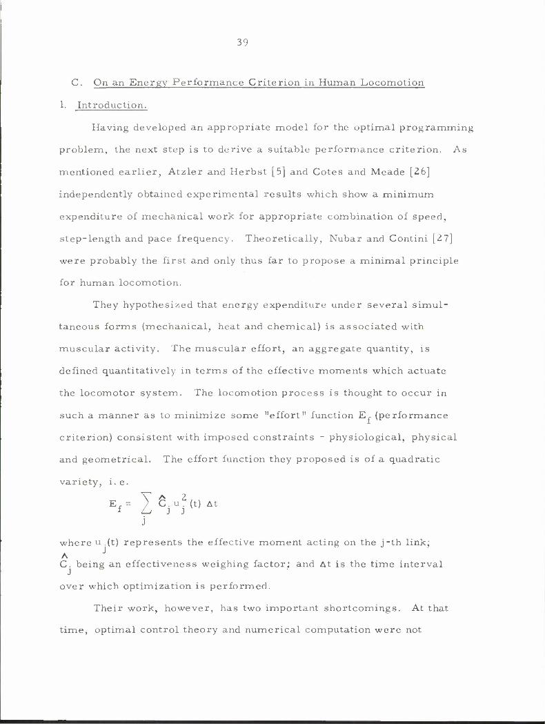
C. On an Energy Performance Criterion in Human Locomotion

1. Introduction.

Having developed an appropriate model for the optimal programming

problem, the next step is to derive a suitable performance criterion. As

mentioned earlier, Atzler and Herbst [5] and Cotes and Meade [26]

independently obtained experimental results which show a minimum

expenditure of mechanical work for appropriate combination of speed,

step-length and pace frequency. Theoretically, Nubar and Contini [2.7]

were probably the first and only thus far to propose a minimal principle

for human locomotion.

They hypothesized that energy expenditure under several simul-

taneous forms (mechanical, heat and chemical) is associated with

muscular activity. The muscular effort, an aggregate quantity, is

defined quantitatively in terms of the effective moments which actuate

the locomotor system. The locomotion process is thought to occur in

such a manner as to minimize some "effort" function E, (performance

criterion) consistent with imposed constraints - physiological, physical

and geometrical. The effort function they proposed is of a quadratic

variety, i. e.

E, = ) C. u . (t) At * Li J J

j

where u .(t) represents the effective moment acting on the j-th link; A J

C. being an effectiveness weighing factor; and At is the time interval

over which optimization is performed.

Their work, however, has two important shortcomings. At that

time, optimal control theory and numerical computation were not

40

developed extensively and the proposed problem was not seriously

tackled. A second and more fundamental question is that while the

effort function being chosen is selected on the basis of mathematical

tractability and physical appeal, there is no apparent connection to the

physiology of the muscle actuating system. Our present objective is

to derive a simple but physiologically based performance index.

2. Development of the Performance Criterion.

Mechanical energy expenditure is the quantity of interest for the

derivation. In general, mechanical work done (by or on) can be

evaluated in two ways. One measure is the time integral of the instan-

taneous power which is the product of the moment about a joint and the

angular velocity of the limb with respect to that joint. The other

measure is the integral of the product the force generated by the

muscle in causing rotation and its velocity of shortening. The latter

method is used as it involves naturally the muscle mechanics.

Specifically, the external characteristics of the muscle are used.

a. Assumptions.

The neural-viscoelastic model for the muscle is based on the

following set of experiments which have been performed on both

isolated muscle fibers and the human muscle in vivo.

(i) tension (force) - velocity curves by A. V. Hill [36, 37]

(ii) length - tension curves [36, 37]

(iii) EMG characteristics by Bigland and Lippoid [46]

Fig. 14 illustrates these properties. From these, the force generated

by a muscle is a function of neural stimulation Z, muscle length £ and

velocity v. The functional form is given as [38, 39]

1 I

uu

cr:

a_ i— \ W ' .INCREASING

STIMULATION LXJ

o \LEVEL

0 Vs Vm

SHORTENING VELOCITY

INCREASING g STIMULATION £

VELOCITY V,/CONSTANT

0 70 85 100115 % OF REST LENGTH TENSI

FIG. 14 EXPERIMENTAL CHARACTERISTICS OF SKELETAL MUSCLES [36,37]

ds « d^ « d

FIG. 15 AGONIST/ ANTAGONIST MUSCLE SYSTEM

42

v F(i,v, Z) = ZFQ(I) f- (1)

1 + b7~ m

where F (£) - maximum isometric force at length £

Z = neural stimulation level (0^ Z ^ 1)

v - maximum velocity for isotonic case (i. e. when F - 0) m i \ i

b = constant (typical values between 0. 25 and 0. 3).

Thus, F is a function of three variables, JC, v, Z. By holding one

variable constant, the muscle length I in this case, F can be graphically

portrayed as a surface. This we call the characteristic surface of the

muscle.

The derivation is confined to one joint agonist/antagonist muscle

system. The actual muscle system involved in almost any complex

limb motion is seldom that simple. We assume that the same principles

hold for each agonist/antagonist pair involved, and thus the discussion

represents an average behavior of all pairs contributing to the actual

limb motion. The human locomotor system is equipped with an abun-

dance of two joint muscles; however, Steindler [4], Eberhart et al [ 10]

have shown how two joint muscles can be functionally decomposed into

the one joint variety,

b. Derivation.

Consider a limb being acted upon by an agonist/antagonist

muscle system (Fig. 15). With the two moment arms approximately

equal, there is no net rotation of the limb when each muscle exerts an

equal force F = Z F (I ). The presence of static forces is to maintain ^ o o o o

joint stability and body posture. When one muscle exerts more force

than the other, a net rotation results. The amount of mechanical work

43

done by the muscle actuating system is given by.

W = (F t 6 F ) • v dt + (F + 6 F.) • v dt U) Jo s s J o r e K '

= \ F (v + v )dt + \ 6 F • v dt + \ 6 F. v dt J ox s e J s s J I e

where 6 F and 0 F are the incremental forces above the static s e

component F in shortening and lengthening respectively. The corre-

sponding shortening and lengthening velocities are v (> 0) and v (< 0).

In normal locomotion, it is taken that |v | •—• jv j and so the static

dependent term F (v + v ) ~ 0, contributing little or nothing to W.

Muscle in Shortening.

From (1), the "shortening" force is

1 --JL V

Fs = ZFo(£) f1 (3)

1 - -2- V m

For normal locomotion activity, F is not significantly different from

the static component so that it can be satisfactorily represented as

6 F = F - F s s o

(z - z) +HT4 (I- I ) + (-^-\ ,aZ / z v o' \ dl J . v o' I 3v I /o

o o / v o

= - Z F (I )(1 +>r)/v o ov o x by m

v o

¥)r° (small)

o

The fact that the linear terms constitute the main contribution is

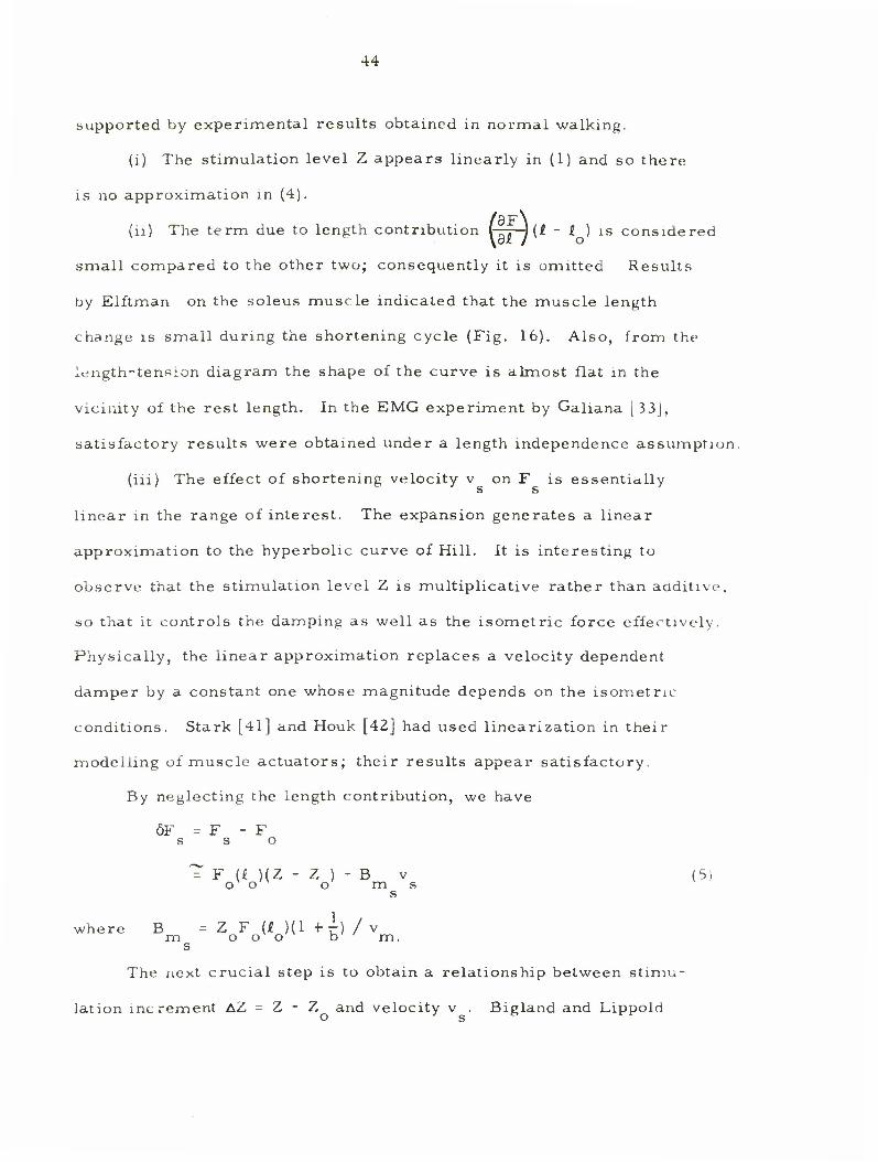
44

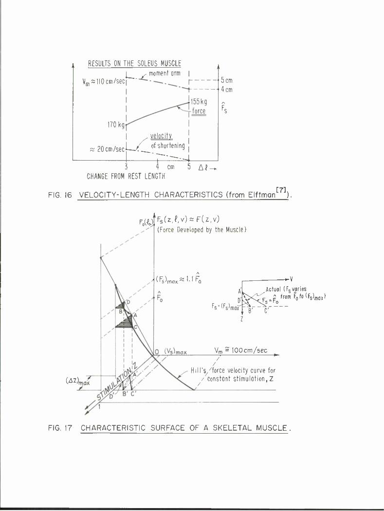
supported by experimental results obtained in normal walking.

(i) The stimulation level Z appears linearly in (1) and so there

is no approximation in (4).

(ii) The term due to length contribution (-• * -) (I - i ) is considered

small compared to the other two; consequently it is omitted Results

by Elftman on the soleus muscle indicated that the muscle length

change is small during the shortening cycle (Fig. 16). Also, from the

length-tension diagram the shape of the curve is almost flat in the

vicinity of the rest length. In the EMG experiment by Galiana [33J,

satisfactory results were obtained under a length independence assumption.

(iii) The effect of shortening velocity v on F is essentially

linear in the range of interest. The expansion generates a linear

approximation to the hyperbolic curve of Hill. It is interesting to

observe that the stimulation level Z is multiplicative rather than additive,

so that it controls the damping as well as the isometric force effectively.

Physically, the linear approximation replaces a velocity dependent

damper by a constant one whose magnitude depends on the isometric

conditions. Stark [41] and Houk [42] had used linearization in their

modelling of muscle actuators; their results appear satisfactory.

By neglecting the length contribution, we have

fiF = F - F s s o

T F (£ )(Z - Z ) - B v (5) o o o m s

s

where B = Z F (I )(1 + H / v m o o o b m. s

The next crucial step is to obtain a relationship between stimu-

lation increment AZ = Z - Z and velocity v . Bigland and Lippold

RESULTS ON THE SOLEUS MUSCLE

Vm = 110 cm/sec l__ , moment orm

170 kg

20 cm/sec

velocity

ot shortening

-I-

5cm 4 cm

Pi

3 4 cm 5 AJ-* CHANGE FROM REST LENGTH

FIG. 16 VELOCITY-LENGTH CHARACTERISTICS (from Elftman1"7-1)

F0(U ovo^

-1 ^'s'max; I-f FA

Fs(z,f,v)sF(z,v) (Force Developed by the Muscle)

F»"(F, s"us'max

-•-V

i^_ Actual (Fs varies

Fs-F0 * from F0to(Fs)max)

„ B' C

Vm = 100 cm/sec

(All 7 Hill's/force velocity curve for

/ constant stimulation,!

FIG. 17 CHARACTERISTIC SURFACE OF A SKELETAL MUSCLE

46

showed that for approximately constant F , v and AZ are linearly

related for small velocities. This is easy to verify from (3):

F v /v \ AZT F-T£T(1 +b)^-oC v8fopM-)«l (6)

o m \ m/

In the normal range of locomotion activity, a linear relationship

between AZ and v still holds but with a slightly larger slope dependent

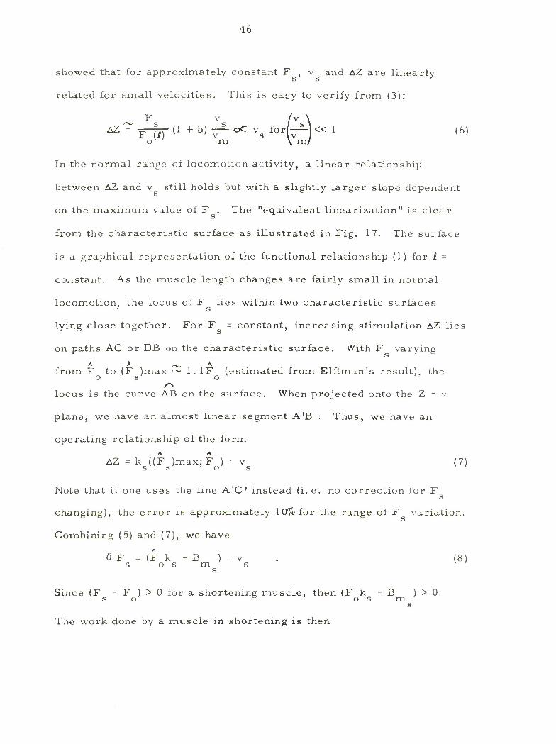
on the maximum value of F . The "equivalent linearization" is clear s

from the characteristic surface as illustrated in Fig. 17. The surface

is a graphical representation of the functional relationship (1) for t -

constant. As the muscle length changes are fairly small in normal

locomotion, the locus of F lies within two characteristic surfaces ' s

lying close together. For F = constant, increasing stimulation AZ lies

on paths AC or DB on the characteristic surface. With F varying A A , A

from F to (F )max ~ 1. IF (estimated from Elftman's result), the o s o r\

locus is the curve AB on the surface. When projected onto the Z - v

plane, we have an almost linear segment A'B'. Thus, we have an

operating relationship of the form

AZ = k ((F )max:F ) • v (7) s s ' o s '

Note that if one uses the line A'C' instead (i. e. no correction for F s

changing), the error is approximately 10% for the range of F variation.

Combining (5) and (7), we have

6 F = (F k - B ) • v . (8) s o s m s s

Since (F - F ) > 0 for a shortening muscle, then (F k - B ) > 0. so o s m s

The work done by a muscle in shortening is then

47

(FC - F r Ws1(Fk -B )dt

os m t o

u2 (t) dt S 1

^

A . 2 2 1 rjt)uc(t)dt (9) (F k -B ) • d (t)

os m s s

•*

t o

where u (t) is the moment generated by the shortening muscle and

d (t) the moment arm. s '

1 , x A 1 2rs(t)= T (10) L S (F k -B )d

os m s s

Muscle in Lengthening.

When the other member of the agonist/antagonist pair is being

stretched, mechanical work is done on it. The Hill's force-velocity

curve holds for the lengthening muscle up to a maximum allowable

force which is roughly twice F (i ). For larger forces, the Golgi

tendon organs reflexly cause the muscle to yield.

Following the same procedure as in the preceding case, the

force in lengthening is given by A

6 F. = F, - F I I o

= F AZ - B v (11) o m- £ v '

B where v. < 0 and £_ ^ , according to Stark, Galiana. Thus,

B ~" m

s

the linear approximation to the characteristic surface is a piecewise

48

one with the damping during lengthening (B ) much larger than that in

shortening. Fig. 18 illustrates that below saturation, AZ and v are

linearly related, i.e.

AZ = k„((FJ : F )v„ (12) £vv I'max' o' i. v '

The work done on the muscle is

rtf * 2 \ <F£ - FQ)

w = . \ ^_o dt

(B -Fk.) J mi ° l t o

%-Fokl>'dfw t o

ltf

I r£(t)u*(t)dt (13) t o

where r«(t) = ^ 2— and d.(t) = moment arm for the

<Bm, " FokM W

lengthening muscle (^ d (t)).

Total Mechanical Work.

The total work done is the sum of lengthening and shortening

contributions

W = W„ + W I s

S*J (rsUs - r^dt" <14> t

o

Bmf ~&Bms

~1.2 F0

FIG. 18 PIECEWISE APPROXIMATION OF CHARACTERISTIC

SURFACE (HOUK[42], STARK[4,], GALIANA[33]).

50

The net moment acting on the limbs is given by

s £ u = _

s

A A (F - F ) - (F - F )

s o e o d

s

d£ '- Us " (d")Ue s

us~u£ for (T") * l • <15> s

2 2 2 2 2 2 Now, u = (u - u.) - u + u. - 2u u. « 2(u +uj v s £ s £ s £ s £

2 2 2 2 But, us - u£^ ug + u£

u = y(u" - uT) ; k = constant factor

h 1 \ , ^ 2 . ,

W = 2 J <rsUs ~r£u£)dt

t o

tf

~ \ 2 = constant • \ u (t)dt . (16)

t o

Hence, in the normal range of activity, the sum total of mechanical

energy expenditure by the muscle activating system is proportional

to the integral of the square of the net moment.

3. Discussions.

In the present derivation, mechanical energy expenditure by the

muscle system is the physical quantity being identified. Although other

quantities such as total energy expenditure by the muscles or total

51

"active states" of the muscles have been suggested as bases for a

performance index, it appears not straight-forward to develop these.

The mechanical work done by (and on) the muscles has been of most

concern in experimental work done to-date.

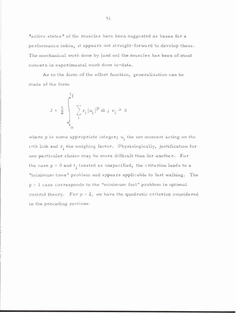
As to the form of the effort function, generalization can be

made of the form

j= | 2"IKIP*J -i

i

t o

where p is some appropriate integer; u. the net moment acting on the

i-th link and r. the weighing factor. Physiologically, justification for

one particular choice may be more difficult than for another. For

the case p = 0 and tf treated as unspecified, the criterion leads to a

"minimum time" problem and appears applicable to fast walking. The

p = 1 case corresponds to the "minimum fuel" problem in optimal

control theory. For p - 2, we have the quadratic criterion considered

in the preceding sections.

5 3

D. Optimization in Biped Locomotion

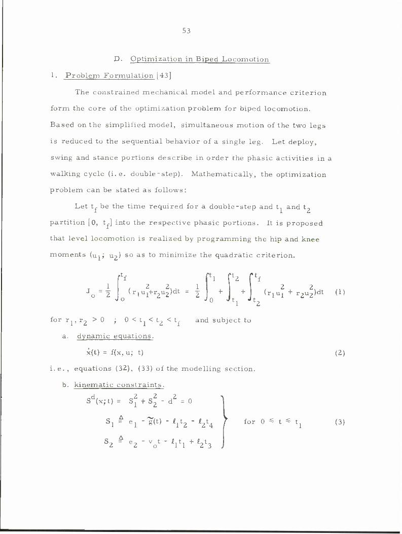
1. Problem Formulation [43]

The constrained mechanical model and performance criterion

form the core of the optimization problem for biped locomotion.

Based on the simplified model, simultaneous motion of the two legs

is reduced to the sequential behavior of a single leg. Let deploy,

swing and stance portions describe in order the phasic activities in a

walking cycle (i.e. double-step). Mathematically, the optimization

problem can be stated as follows:

Let tf be the time required for a double-step and t, and t?

partition [0, t,] into the respective phasic portions. It is proposed

that level locomotion is realized by programming the hip and knee

moments (u, ; Uo) so as to minimize the quadratic criterion.

.t,

1 . 2 2., 1 \ r^ u^+r^u^dt ~ ?

1

+ 0 JtL

ft,

Jt. (rlUl + rzu2)dt (1)

for r,, r-> > 0 ; 0 < t. < t2 < t, and subject to

a. dynamic equations.

k{t) - f(x, u; t)

i.e., equations (32), (33) of the modelling section.

b. kinematic constraints.

Sd(x;t) = S^ + s\ - d2 = 0

;i = ei "^ ~ hh • V-

S7 = e7 " v t - ft. 4- £ t_ c. L o 11 c. 3 j

for 0

(2)

(3)

S4

SS(x, t) = g(t) + llt2 + £zt4 + dcos(3 - e

(3 2 Ti - 5 max

cj) 4- x, o 1

x2 >0

for t.<t< t2

for t2<t^t Sj (x;t) = g(t) + Ij^ + *2t4 + p(t) - eQ = 0

S£s (x;t) = vQ(t + tQ) + £1t1 - £2t3 - q(t) - 0

initial and terminal conditions.

x(0) = x (specified)

Y 1(x(t1);t1) * [Sd(x;t)]t = t = (sf + S2 - d2)t = 0

S^Wt^V ^x2(tl) - xl(tl) + 4Q + 6max -f - a(tl) =0

These are the terminal hypersurface constraints for deploy.

A A x(t2) = x2 ~ d (specified)

x(tf) = x(0) (repeatability in walking)

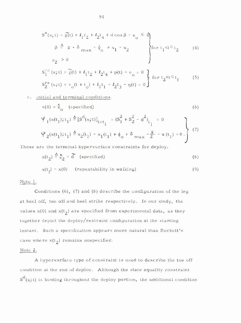
Note 1.

(4)

(5)

(6)

(7)

(8)

(9)

Conditions (6), (7) and (8) describe the configuration of the leg

at heel off, toe off and heel strike respectively. In our study, the

values x(0) and x(t?) are specified from experimental data, as they

together depict the deploy/restraint configuration at the starting

instant. Such a specification appears more natural than Beckett's

case where x(t?) remains unspecified.

Note 2.

A hypersurface type of constraint is used to describe the toe off

condition at the end of deploy. Although the state equality constraint

S (xjt) is binding throughout the deploy portion, the additional condition

55

Vf , = 0 is a device used to eliminate possible jumps for the influence

equations in numerical simulation. The Y - 0 condition describes

"foot-locking" for the subsequent swing; and 6 max, a (t. ) are set at

110 and 70 for simulation [10].

Note 3.

The condition (9) describes repeatability of motion in normal

level walking.

Note 4.

From the kinematic constraints (3) describing deploy motion and

Fig. 12, we can write

Sl ~ el " g^ " <L\t2 " £2t4 = dsina

S = e, - v t - £,t. + It = dcosa 2 2 o 11 2 3

where d = effective length of the foot between the ankle joint and

the ball of the foot (i. e. center of rotation)

;. tana = (-gJ-J ^=> a (t) = tan" V ^J

Sl a(t) = -5±- b2

Sl S1S2 a (t) = -s— - -o

2 S2

2. Characteristics of the Problem Formulation

a. It is a programming approach as opposed to the direct approach

taken in other studies.

b. The formulation results in a multi-arc programming problem

with three stages on account of the varied nature of the ankle reactions

and moments; kinematic constraints; initial and terminal conditions.

56

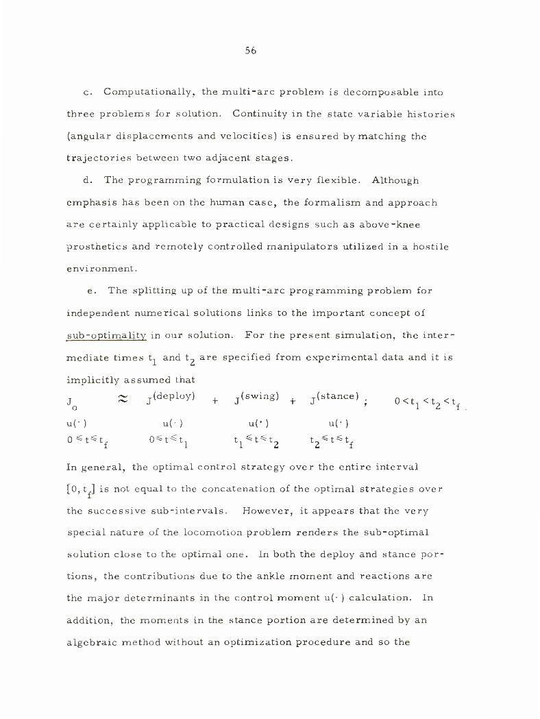
c. Computationally, the multi-arc problem is decomposable into

three problems for solution. Continuity in the state variable histories

(angular displacements and velocities) is ensured by matching the

trajectories between two adjacent stages.

d. The programming formulation is very flexible. Although

emphasis has been on the human case, the formalism and approach

are certainly applicable to practical designs such as above-knee

prosthetics and remotely controlled manipulators utilized in a hostile

environment.

e. The splitting up of the multi-arc programming problem for

independent numerical solutions links to the important concept of

sub-optima lit y in our solution. For the present simulation, the inter-

mediate times t, and t? are specified from experimental data and it is

implicitly assumed that

' }; 0<ti<t2<tf

"f

In general, the optimal control strategy over the entire interval

[0,t ] is not equal to the concatenation of the optimal strategies over

the successive sub-intervals. However, it appears that the very

special nature of the locomotion problem renders the sub-optimal

solution close to the optimal one. In both the deploy and stance por-

tions, the contributions due to the ankle moment and reactions are

the major determinants in the control moment u(- ) calculation. In

addition, the moments in the stance portion are determined by an

algebraic method without an optimization procedure and so the

J o <~w j\ut^iuy/ + y \ O W A 1J. ti / + j*-"""-

u(-) u(-) u(') u(-)

0<t«tf 0^t«tj t ^t^t ll L2 t^t

57

., T(stance) . „ , contribution J is essentially constant, irrespective of

optimization. The cost J is a small fraction of the total

cost because the subinterval [0, t, ] is short (i.e. -— ^ 0 1 to 0. 1 5) f

and the control moments are also influenced by the ankle moment and

^A i ., T(swing) . . ,. ., . . reactions. Only the term J ° can be significantly minimized

via optimization. Thus, it appears that the sub-optimal solution

should be very close to the true optimal.

3. Necessary Conditions of Optimality; Method of Solution.

With the problem formulation completed, the next step is to

invoke the necessary conditions of optimality. Solution for the deploy

and swing portions are first considered as they are of a similar

nature. The technique is to convert the original constrained optimi-

zation problem into a sequential unconstrained problem. Let S(x; t)

denote the state constraint (equality or inequality) in either portion.

Define an extra state variable Xj-(t) such that it satisfies the differential

equation

x5(t) = sgn(S) • S2(x;t) (10)

sgn(S) # )

for O^t^t,; t.^t*-t?. The original state vector satisfies, of

course, the dynamic equation

T x(t) = f(x, u,-t) ; x = (xj, x2, x^, x4)

With the initial condition set to zero, i. e. x-(t, ) = 0 for swing

x,-(0) = 0 for deploy respectively, then

Sgn(S)S2(x;n)dn - 0 (13)

=*> Sgn(S) • S2(x; n) = 0 Vne[0, tj or ne[t1, t-,] .

The state constraint is thus satisfied. A mathematical proof of the

above penalty function technique is given by Lele and Jacobson [44].

As far as the initial and terminal conditions are concerned, a

quadratic penalty function is used. With these, the necessary condi-

tions of optimality can be separately derived for the deploy and swing

portions.

In deploy, we have the modified performance criterion for the

sequential unconstrained problem, i. e.

Min Jd = cr k(x5(t1) + ty ^(t^tj) + ^^V'V + (x3(tl)_d3)2

u

+ (x4(t1) - d4)2} +-|\ (rlU2 + r2u2)dt . (14)

Specifically, we solve (14) for a monotonically increasing sequence

0< or < or < <(rv an<^ subject to the equations

x(t) = f(x,u;t) ; x(0) = x^

\ (15)

k5(t) = (Sd(x;t))2; x5(0) = Oj .

The signum function Sgn(S ) = 1 because the state equality constraint

is effective throughout the interval. Define a variational Hamiltonian

k' H (x, u, X, cr • t) as

Hd = ^(rju2 + r2u2) + ) \.f.(x,u;t) + X^t) (Sd(x;t))2 (16)

j=l

The X's are the influence functions or the adjoint variables of the

59

optimization problem. The extremal condition is

4 du 9f.

= 0 =»r.u. + > X. TH~ = 0 for i = 1, 2 . 3u. l l L, J 8u.

j = l

(17)

riu1+-(A2X3+t7X4) = 0

r2u2 + 6(t7X3+t8K4) = 0

(17a)

a2Hd Note: -s-" = r. > 0 for r. > 0: i = 1,2. The influence equations 2 I I '

9u.

and their terminal conditions at t, are

i 9x.

i=l

-,4

-\c = 0 5

J

a^ W = 2ffk(^i id-+,//

9^2

Z 9x2

X3(tl} = 2(r k(x3(V " d3)

W = ^k^V " d4)

\S(tl) = (rk k

/ (18)

as' Explicitly, expressions for the \-equations and -y are given as follows

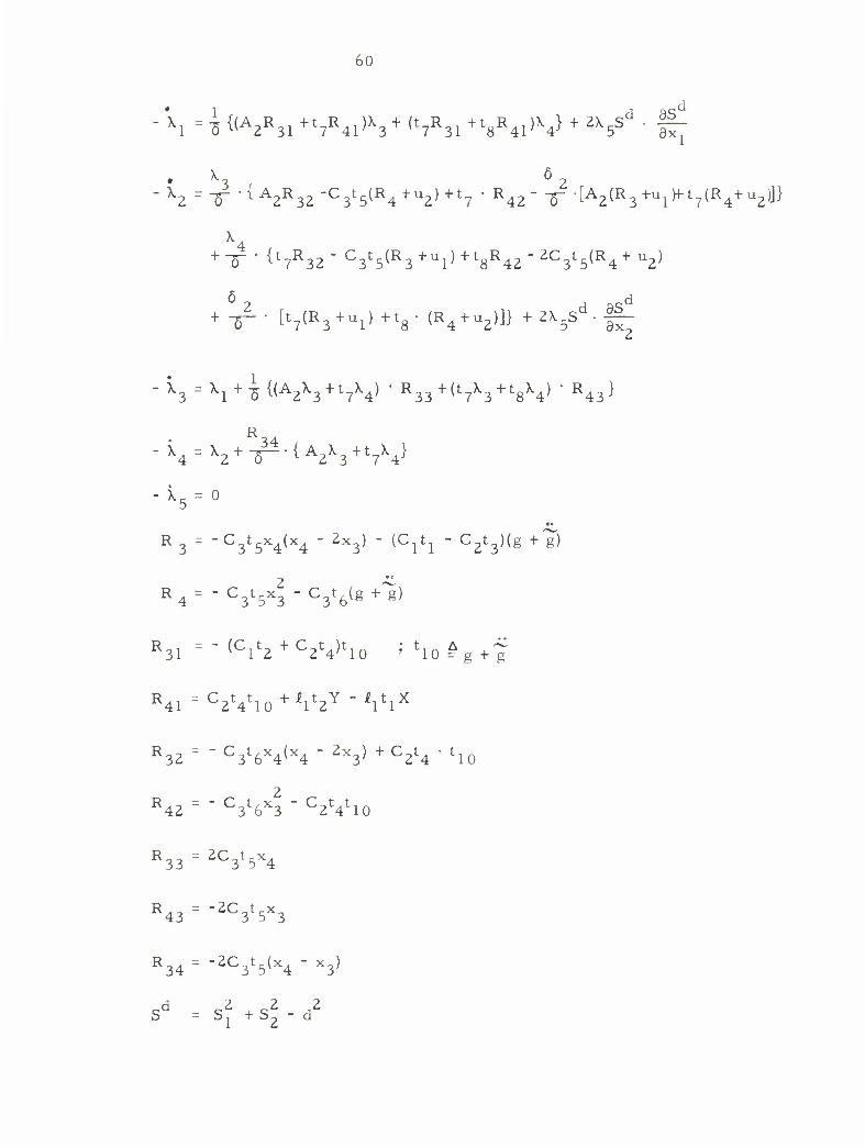
60

\ - Z «A2R31 +t7R41)X3+ (t7R31 + t8R41>V + Zk 5S* ' f"

• S X2 = ~5^ { A2R32~C3t5(R4*u2)+t7 ' R42 " "5" [A2(R3 +ul ^ t7(R4+ u2^

\ + ~5~ " {t7R32" C

3t5(R3+ul)+t8R42~2C3t5(R4+ u2>

6 ? rf a<?d

+ -^~ • [t7(R3+Ul) +t8- (R4 + u2)]} + 2X5Sa- |f >x.

X3 = X1 + ^{(A2X3+t7X4) • R33 + (t?\3+t8X4) • R43}

R 34

^'VT^VS+W X = 0

b

R C3t5x4(x4 " 2x3} ' ^lh " C2t3)(g + g)

R4=-C3t5x3-C3t6(g + g)

R31 =- (C^+C^t^ ; t1QAg+~

R41 =C2t4t10+£lt2Y "VlX

R32 = " C3l6x4{x4 " 2x3) + C2fc4 ' 'lO

R 42 C3t6x3 " C2VlO

R33 = 2C3t5x4

R43="2C3t5X3

R34 = -2C3t5(x4 - x3)

2 2 2 S^ +s2 - d

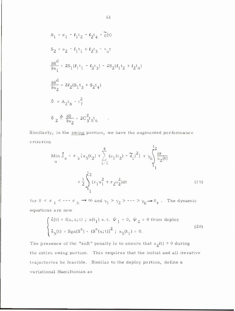
61

si =ei "Vz ' lzh "8(t)

S, = e-, - £,t, + £0t. - v t L L 11 Z 3 o

|^=2S1(£1t1-V3)-2S2U1t2+V4)

H-- 2l2(Slt3 + S2t4)

* 2 6 = A2l8 " <7

6 2 * ^ = 2C3'5'6 '

Similarly, in the swing portion, we have the augmented performance

criterion

4 iz Min Js = , k{x5(t2) +^ (Xl(t2) - d.)2} + YA f-^

u i=l J Z

2 )(rlul f t ) (rlul + r2u2)dt (19)

forO < cr, < o- 00 and Yi > Y? > > Yi,--¥ 0+ • The dynamic

equations are now

x(t) = f(x,ujt) ; x(tj) s. t. ^ 1 = 0, l//2 = 0 from deploy

2 <20> x5(t) - SgntS") • (Sa(x;t)r i x^t^ 0.

The presence of the "soft" penalty is to ensure that x2(t) > 0 during

the entire swing portion. This requires that the initial and all iterative

trajectories be feasible. Similar to the deploy portion, define a

variational Hamiltonian as

62

HS(x,u,X;o-k, Vt)^i(rlUf + r2u^) + ^ + 2Xjfj(x'U;t)

+ K5(t) • Sgn(SS) (SS(x;t))Z . (21)

Again, the extremal condition implies

4 9f.

(HS)u=0=»r1u1 ^^-^ = 0; i = l,2 . (22)

The equation set (17a) is thus obtained. The influence equations and

their appropriate boundary conditions are

( ^ 9f. -X. = ) X. -—L+ 2\I.Sgn(SS) • S

l /_, j 8x. 5 fo

ass Yk-6(2,i) "N

i=i

•X = 0

K.(t2)-2ak(x(t2)-d.)

\5(t2) = a k

ax. 2 1 x2(t)

F (23)

J for i = 1, ,4 and 6 (2, i) = 1 if i = 2 and 0 otherwise. The expressions

for the X-equations are similar to those for the deploy portion except for

the substitution of inequality for equality constraint expressions.

Expressions related to the constraint are

"as! 9x,

as: < 8x-

-j^tj + £2t - d sin P(t)

•£2t + d sin P(t) (24)

I - 0: !§- = 0 ax. ax,

63

For both the deploy and swing portions, we thus have a two-point

boundary value problem (TPBVP) (15, 17a, 18) and (20,22,23)

for the respective unconstrained optimization problems.

Solution of the stance portion differs from the other two stages.

The leg in stance carries the body weight while the inertia of the

trunk and forward motion of the swinging leg carry the entire body-

forward. The result is a "sinusoidal" trajectory for the hip and the

foot is almost stationary during the roll-over. With prescribed

motion for the hip and ankle, motion of the thigh and shank are

determined through these kinematic constraints. The result is that

the effective hip and knee moments can be found without the need of

minimization of the performance criterion; an algebraic method is

sufficient for the solution in this portion. The equality constraints

on the ankle motion are

S[s(x;t) =^(t) + £ltz + £2t4 + p(t) - eQ = 0

S^x^t) = vQ(t + tQ) + £]t1 - £2t3 - q(t) = 0

for t? ^ t ^ t,. Differentiating once with respect to t, we have

(51)

S[s(x;t) = g-(t) + p(t) +• znx3 + z12x4(t) = 0

S2rS(x;t) = VQ - q(t) -r z2l

x3<t) + z22X4(t) = °

(25)

where

/zn ziz\ rVi+Va "V3

VZ21 Z22 / \ ^^2 + f2l4 " V^

The equation sets (5') and (25) form a decoupled system of four

equations in the state variables (x, , , x ) at each instant of time in

64

the stance interval. Note that (5 ) is a nonlinear equation set in x,

and x, while (25) is linear in x and x with the coefficients z Z 5 4 ij

(i, j = 1,2) as functions of x, and x->. Differentiating once more with

respect to time,

••rs \szJ

/ '—• •• / g + P

+ Z - L

/ Z X3

V(x4"x3)J

(26)

where It

Vi

t.\ 2 4

" Vay Now, x, and x. contain the actuating moments u. and u? explicitly

from the original dynamic equations

/ xl = x3

x2 " x4

x3 = - {A2(iT3 +Uj +Ma + (i1t1 "i2t3)Y +(I1t2+l2t4)X) + t7(R4

+ u2-Ma+£2t3Y-i2t4X)} (27)

x4 = -{t7(R3+Ul +Ma + (I1t1 -i2t3)Y +(jJ,t2+i2t4)X) + t8(R4+u2

V -Ma+£2t3Y -£2t4X)}

or

R

\R4

+ A

\U2

A"1 --1

' A "6

I A,

W A.,r -t

2 8 7

(27')

Combining (26) and (27'), the moments can be expressed as:

65

A R ( *

\ X3 " (g + P)1

A + AZ L

VR4/ >4-x3) I 'q(t)

V (2s>

/

M and = Z L

' X3

(x4 " x3)

(T+P)

\ q(t

J

(29)

To generate the trajectories in the stance portion, we proceed

forward from t = t~ to t = t, in small positive increments, A. At each

instant, solve equation set (5') for x and x? numerically (this is

essentially finding the roots of nonlinear equations). With the x. and

x? values determined, the matrix Z is known and so the variables x.,

and x. can be computed from (25). Equation (28) then generates the

hip and knee moment profiles.

0 7

E. Numerical Simulation and Results

1. Parameters and Pertinent Data

Having formulated an optimal programming theory for biped

locomotion, the next step is to perform a numerical simulation of the

gait based on the proposed theory. This is a crucial step because

only the results can demonstrate the validity and relevance of the

theory. In general, the walking pattern of each individual is a little

different from that of another person because of the skeletal structure

and physiological conditions. However, there are characteristic,

qualitative features which are observable in the human gait for non-

pathological cases. The objective of the numerical experiment is to

simulate these common features,

a. Physical Parameters.

The values of the parameters used in the present computation

are based on those used by Galiana and Milsum [33] in their EMG-

experiment. Typical values for the mass, length and moment of

inertia for the two segments of the lower extremity are listed as

shown below. It is noted that their values are derived from the

commonly used "percentage" values of Fisher and Dempster in

Lissner [32]. Values of the composite parameters used in the mathe-

matical model are also listed.

Parameter Value Remarks

Body Weight, W 130 pounds

Mass, A 4. 05 slugs A = w/g

Mass of Thigh, Mj 0. 389 slugs 9- 6% of A

Mass of Shank, M? 0.2595 slugs 6. 4% of A (includes mass of ° foot)

68

Parameter Value Remarks _2

Moment of Inertia of Thigh, I, 1.4x10 slugs

-2 Moment of Inertia of Shank, L 1.882x10 * slugs (shank-foot combination)

Link Length of Thigh, J^ 1. 3524282 ft.

Link Length of Shank, t^ 1.2618726 ft.

Distance from Hip Joint 0. 586 ft. Dempster's average data

to C. G. of Thigh, a 1

Distance from Knee Joint 0. 547 ft. Dempster's data

to C. G. of Shank, a ?

(*) Length of Foot 0. 55 ft. Effective length in deploy

0. 65 ft. Effective length in swing

Composite Parameters in Simulation

2 2 2 A, = I, + mja . + mzJ?1 = 0. 5993547648 slug-ft.

A2 = !2 + m2a 2 = 0. 1414525055 slug-ft. 2

Cl = mla 1 + m2£l = 0. 564730024 slug-ft.

C2 = m2a2 = 0. 1735743239 slug-ft. 2

C3 = C2 • il = 0. 2347468104 slug-ft. 2

b. Initial and Terminal Conditions.

The starting values for the angular displacements and velocities

(i. e. initial states) are derived from Beckett's [28] numerical experi-

ment These are

(*) During deploy, the foot rotates about its ball. The distance between the ankle joint and center of rotation is shorter than the foot-length during swing when the toes are also taken into consideration.

69

x (0) = 0. 11170107 radians (6. 4°)

x2(0) = 0.2268928 radians (13°)

x (0) = x,(0) = 0. radians/sec.

x.(0) = x?(0) = 1. 68 radians/sec.

At the end of the double-step, the terminal values are chosen as

x (2. 0) = 0. 799 radians (46°)

x2(2. 0) ~ 0. 052 radians (3°)

x,(2. 0) = 0. 0 radians/sec.

x.(2. 0) : 0.0 radians/sec.

The initial, intermediate and terminal times for the three portions

are set at t - 0; t, - 0. 2 sec (deploy); t2 = 1.0 sec (swing); t, = 2. 0

(stance). Here, we assume a 10% interval for deploy and restraint

activity. The swing (or support) occupies 40%. Variation in the

temporal patterns modify the numerical results but not the methodology

c. Prescribed Trajectories.

For the hip motion, we have

T(t) - v (t + t ) feet o o

v = 2. 275 ft. /sec. o

t = 0. 24698953 sec. o

7(1) = eQ - JJ- sin ^- (t + |3 • tf) feet

e = 2. 7358172 feet o

t, = 2.0 sec.

(3 = 0. 525

70

e, = e = 2. 7358172 feet 1 o

e, = - v t = - 0. 399078 feet L o o

To describe the almost stationary behavior of the foot in stance

portion, we rely on the experimental profiles by Bresler and Frankel

[13], and other experimenters [10, 12], (Fig. 11). For the present

simulation, simple curve fitting on the experimental data is used as

our important objective is to illustrate our approach of study. Better

results could be obtained through interpolation or spline function

approximation. In the stance portion simulation, the following prescribed

trajectories are used for the ankle motion:

q(t) = 2. 00+ 0.35(l-e"6'5 ); T#t-1.0;1.0^t<2. 0.

JO. 1 7 -f- 0. 1 5 Sgn ( n ) • n2 1. 0< t< 1. 3

p(t) ={0. 17 1. 3<t^ 1. 55

0. l7 + 0.25(t-l. 0)+49. 1 • [0. 25(t-l)4- 0. 755(t-l)3

+ 0.8 5(t-l)2 - 0. 421 (t-1)] 1. 55<t ^2. 0

j^t-0.3 ; Sgn(n) = {J J %\

The particular choice of (p, q)-profiles is based on the form of the

experimental curves as well as continuity at the matching points,

d. Pressure Transfer Curve.

Equation (46) of mathematical modelling proposes a linear

expression for the transfer characteristics of the pressure center in the

stance portion. The distance travelled from heel strike to rotation about

the ball of the foot is equal to the effective foot length in deploy, i.e.

d = 0. 55'. In approximately mid-stance, the ankle joint is directly

above the pressure center. These two pieces of information give us

71

the required expression:

x (t) = 2. 35 + 0. 9 (t - 1. 40) feet 1. 0 ^ t < 2. 0

2. Numerical Computations.

From the conditions of optimality, a first order algorithm is

employed for iterative, numerical solution. The algorithm is coded into

Fortran IV programming language to run on the IBM 360/65 digital

computer. The program possesses the following features:

a. The program has two options:

(1) a one-dimensional minimization subroutine (QUADCL) used in

conjunction with conjugate gradient or steepest descent algorithms.

(2) a simple gradient procedure with a pre-specified improvement

step-size.

b. A fourth order Runge-Kutta method with fixed integration step-

size is used for integrating the state and adjoint equations. In each

integration step, the control histories u(t), state trajectories x(t) and

ground reactions (X(t), Y(t)) are represented by their values at the end

points. Presumably, such a "discretization" could have effect on the

quality and convergence rate of the computation.

c. To satisfy the state constraints, the computation is done in

series with increasing positive values of the weighing factor, cr .

d. The computation is carried out in single precision arithmetic.

The numerical computation is involved because the dynamic

equations involve five state variables and they are highly non-linear.

More efficient algorithms such as second order optimization methods

are very complicated to program. In the literature, little has been

reported on the computational experience involving problems of such

72

complexity. Besides, the primary purpose of the computation is to

establish the relevance of the theory to biped locomotion and simulate

the common features of gait. These considerations prompt the use

of the first order algorithm for an adequate, approximate solution to

the problem. For each value of cr , the computation involves a large

number of iterations before a satisfactory solution is obtained. The

procedure with the QUADCL-search option involves more computing

time per iteration in general than the simple fixed-step gradient

procedure. However, these two options were used more or less

alternatively to achieve improvement (cost reduction) because of the

non-linearity of the problem. An acceptable solution is obtained with

3 2 cr =10 for the deploy portion and cr =10 for the swing. An

interesting observation is that the swing portion with an inequality

constraint is comparatively simpler to compute than an equality

constraint as in the deploy portion.

3. Results and Discussion.

Results of the simulation are summerized in the various graphs.

To facilitate discussion, comparison is made with the often-quoted

experimental works of the Eberhart-Inman group at Berkeley [10, 12,

13]. In general, the results can be classified into three groups for

discussion.

a. Angular Displacements and Related Results.

Results pertaining to this part are depicted in the graphs No. 1

to No. 7. The state trajectories x, (t) and x?(t) together with their

time derivatives portray the angular motion of the thigh and shank in

the sagittal plane. Note that the curves are so plotted that they begin

7.5

at heel strike (i.e. stance portion) for comparison purposes.

The x?(t)-trajectory describes the motion of the shank with

reference to the thigh. At heel strike, the knee joint is extended

so that the x^tt) angle is at a small positive value. During the brief

restraining portion of stance, the angle x? increases so that this flexing

of the knee absorbs the impact of body weight passing on to the leg in

stance. The angle then decreases until deploy when it starts to increase

rapidly. The behavior that the knee is first flexed at heel strike and

then flexed again during deploy is known as "knee locking" - a fact well

documented in experimental studies. In the swing portion, x-,(t) reaches

a peak value of roughly 80° and then decreases rapidly to almost zero

in 0. 5 second. The behavior resembles the ballistic action of a

pendulum as illustrated clearly by the velocity profile x?(t) in graph

No. 2. In the pioneering works of Fischer, it was conjectured that the

action of the leg in swing is purely due to gravity, but this was disputed

by others later in connection with muscle activity studies. From the

present optimization standpoint, it appears that the effective moments

cooperate with gravity for lesser expenditure of work while still

satisfying the state constraints. From the graph No. 17, it is apparent

that the constraint is well satisfied. The state trajectories (i. e.

angular displacements and velocities) are well matched for the multi-

arc programming problem. This is achieved by using the terminal

conditions of one stage as the initial values for the following in actual

computation. However, there exist small discontinuities for the

acceleration and moment profiles at the stance/deploy and deploy/swing

junctions. The reason for the mismatch is primarily numerical as the

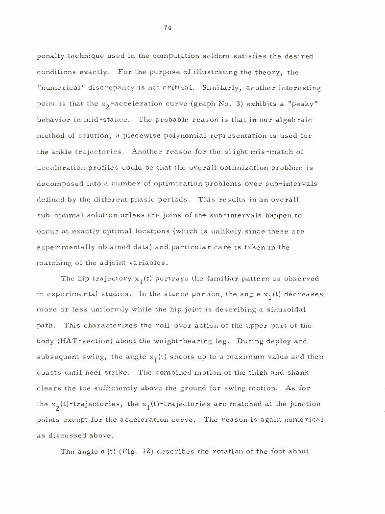
74

penalty technique used in the computation seldom satisfies the desired

conditions exactly. For the purpose of illustrating the theory, the

"numerical" discrepancy is not critical. Similarly, another interesting

point is that the x2"acceleration curve (graph No. 3) exhibits a "peaky"

behavior in mid-stance. The probable reason is that in our algebraic

method of solution, a piecewise polynomial representation is used for

the ankle trajectories. Another reason for the slight mis-match of

acceleration profiles could be that the overall optimization problem is

decomposed into a number of optimization problems over sub-intervals

defined by the different phasic periods. This results in an overall

sub-optimal solution unless the joins of the sub-intervals happen to

occur at exactly optimal locations (which is unlikely since these are

experimentally obtained data) and particular care is taken in the

matching of the adjoint variables.

The hip trajectory x, (t) portrays the familiar pattern as observed

in experimental studies. In the stance portion, the angle x, (t) decreases

more or less uniformly while the hip joint is describing a sinusoidal

path. This characterizes the roll-over action of the upper part of the

body (HAT-section) about the weight-bearing leg. During deploy and

subsequent swing, the angle x, (t) shoots up to a maximum value and then

coasts until heel strike. The combined motion of the thigh and shank

clears the toe sufficiently above the ground for swing motion. As for

the x (t)-trajectories, the x, (t)-trajectories are matched at the junction

points except for the acceleration curve. The reason is again numerical

as discussed above.

The angle a (t) (Fig. 12) describes the rotation of the foot about

75

its ball during deploy action. Graph No. 4 shows the result of

computation based on the equality constraint relationship. The angle

a (t) has a monotonically increasing profile, reaching a limiting value

of about 1. 2 radians (— 68°) at the end of deploy. A value of 70° was

used for specifying the terminal deploy conditions. The velocity and

acceleration curves likewise show a monotonically increasing trend,

but the acceleration trajectory appears to be more irregular. This is

because the state constraint is satisfied approximately as shown in

the residue error curve in graph No. 16.

The angular displacements, velocities and accelerations con-

stitute the main results of the computation upon which related quantities

can be calculated. Graph No. 5 shows a phase plane diagram for the

angular displacements x. (t) versus x?(t) during a double-step. In the

paper by Marie and Vukobratovic, a special type of compass gait was

considered in which the hip motion is stationary in the vertical direction

and the foot is in continuous contact with the ground. The resulting

realization of the gait pattern is that the thigh and shank angles are

sinusoidal in a double-step. This gives an elliptic phase plane plot

with the points equally spaced. The present results simulate much more

realistically the biped gait and the plot indicates deformation of the

curve in the stance portion. Note that the points are not uniformly

spaced, showing different rates of activity in the three portions.

The horizontal and vertical displacements of the joints are

plotted in graphs No. 6 and No. 7. A double-step takes two seconds

during which there is an overall horizontal displacement of 4. 55 feet.

This gives a walking speed of about 1. 6 miles per hour, a case of slow

76

level walking. The hip moves at a uniform rate while the knee and

ankle move through 4 feet during the swing portion. Graph No. 7

illustrates the vertical displacement of the joints. A double sinusoid

with 0. 9 inches in amplitude is used to simulate the hip motion. In a

more accurate description, a Fourier series representation can be used

to fit the experimental profile. In fact, the amplitude and phase of the

various components have been studied to reveal the abnormal properties

of the pathological gait. In the normal case, the double sinusoid is the

principal component. During stance, the knee joint is almost stationary,

so is the ankle trajectory as prescribed by the p(t)-profile. The

displacement at initial stance is prevailingly restraining action to

absorb impact and the gradual increase towards deploy implies the

transfer of the pressure center. In subsequent deploy and swing motion,

the vertical motion of the knee and ankle is comparatively larger. Note

that the overall vertical displacement is almost zero in a double-step.

b. Reaction Forces and Moments at the Joints.

The foregoing section describes the kinematic behavior of the

lower extremity in level walking. To complete the description,

dynamic quantities such as the forces and moments at the various joints

must be determined. It is only with the dynamic information that a

realistic description of biped locomotion can be said to have been

achieved. In the weight bearing portions, the foot is subjected to very

large ground reaction forces due to the weight and acceleration of the

upper part of the body (HAT-section). With these large forces

appearing at the inputs to the dynamic equations, it is not difficult to

realize that they are the dominant quantities in determining the

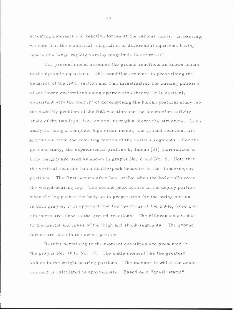
77

actuating moments and reaction forces at the various joints. In passing,

we note that the numerical integration of differential equations having

inputs of a large rapidly varying magnitude is not trivial.

The present model assumes the ground reactions as known inputs

to the dynamic equations. This condition amounts to prescribing the

behavior of the HAT-section and then investigating the walking patterns

of the lower extremities using optimization theory. It is certainly

consistent with the concept of decomposing the human postural study into

the stability problem of the HAT-section and the locomotion activity

study of the two legs, i. e. control through a hierarchy structure. In an

analysis using a complete high order model, the ground reactions are

determined from the resulting motion of the various segments. For the

present study, the experimental profiles by Inman [31] (normalized to

body weight) are used as shown in graphs No. 8 and No. 9. Note that

the vertical reaction has a double-peak behavior in the stance-deploy

portions. The first occurs after heel strike when the body rolls over

the weight-bearing leg. The second peak occurs in the deploy portion

when the leg pushes the body up in preparation for the swing motion.

In both graphs, it is apparent that the reactions at the ankle, knee and

hip joints are close to the ground reactions. The differences are due

to the inertia and mass of the thigh and shank segments. The ground

forces are zero in the swing portion.

Results pertaining to the moment quantities are presented in

the graphs No. 1 0 to No. 12. The ankle moment has the greatest

values in the weight bearing portions. The manner in which the ankle

moment is calculated is approximate. Based on a "quasi-static"

78

assumption, the inertial and gravitational effects of the foot are

neglected as they are l%or less of the contribution of the ground

reactions. In addition, a linear function is used to describe the

transfer of pressure center in stance. Despite the crudeness of the

calculation, the ankle moment agrees qualitatively well with the

experimental results of Bresler and Frankel [13]. This is encouraging

because the approximate calculation avoids the complexity of the high

order model. With better representation (e. g. spline polynomial

interpolation) of the prescribed trajectories, better results are antici-

pated. The ankle moment and ground reaction contributions are the

dominant quantities in determining the hip and knee moments in the

stance and deploy portions (graphs No. 11 and No. 12). This is very

interesting because the inertial and gravitational terms are the most

complicated to calculateand yet they are only second in importance in

the moment calculation. Thus, the use of the simplified decoupled

model together with kinematic constraints is not as crude as it may

initially appear. However, neglecting the ankle moment and ground

reactions makes a big difference in the moment calculation. This,

then, should explain the shortcomings of the papers by Beckett,

Wallach, Galiana and Vukobratovic et al.

The hip and knee moments are also plotted in graph No. 10.

The greatest activity occurs during stance following heel strike and

at deploy. Activity in the swing portion is addressed to maintaining

the leg above the ground (i.e. to satisfy the state inequality constraints)

while utilizing gravity as much as possible).

The knee moment profile shows a typical pattern associated with

7<J

the "knee-locking" behavior discussed earlier in a. The sign

convention for the moment is such that, when negative, the forces

pass behind the knee, tending to flex it; while a positive moment

tends to hold the knee in a "locked" position. The present profile

agrees fairly well with experiment [13]. At heel strike, the leg is

quickly stabilized, then unlocked, and once again locked for the

deploy portion. Bresler [13] pointed out that the knee-locking behavior

allows one to move forward with a minimum raise of center of gravity,

and therefore less expenditure of work.

Like the ankle and knee moments, the hip moment again agrees

with the experimental pattern. The negative moment following heel

strike is responsible for the roll-over of the body, indicated by a mono-

tonic decrease of the x1(t)-ankle. Toward the deploy, the hip angle

starts to increase. The greatest values at initial stance and deploy

are opposite in sign. Based on the idea of two basic configurations for

the biped gait, the two portions of "maximum" activity correspond to the

"restraint/deploy" configuration (Fig. 6). From the dynamic equation

for the HAT-section, the trunk of the body is subjected to the action of

the hip moments. But the interesting fact that the hip moments of the

two legs are more or less of the same order of magnitude but opposite

in sign leads to the concept of moment annihilation (i. e. cancelling) of

the hip moment's effect on the HAT-section. This consequently requires

far less stabilizing moment effort for maintaining up-right posture.' In

the same vein, the "complementary" * profiles for the hip reaction

forces (graphs No. 8 and No. 9) create a couple action in the frontal

f i.e. , the profiles at deploy are reflections of those at initial stance.

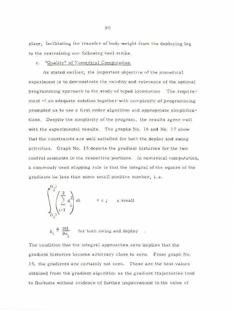
80

plane, facilitating the transfer of body weight from the deploying leg

to the restraining one following heel strike,

c. "Quality" of Numerical Computation.

As stated earlier, the important objective of the numerical

experiment is to demonstrate the validity and relevance of the optimal

programming approach to the study of biped locomotion The require-

ment of an adequate solution together with complexity of programming

prompted us to use a first order algorithm and appropriate simplifica-

tions. Despite the simplicity of the program, the results agree veil

with the experimental results. The graphs No. 16 and No. 17 show

that the constraints are well satisfied for both the deploy and swing

activities. Graph No. 15 depicts the gradient histories for the two

control moments in the respective portions. In numerical computation,

a commonly used stopping rule is that the integral of the square of the

gradients be less than some small positive number, i. e.

.<v _2

2

> <\« < € ; e small

I = 1

A fiH g. = —— for both swing and deploy

l du. l

The condition that the integral approaches zero implies that the

gradient histories become arbitrary close to zero. From graph No.

15, the gradients are certainly not zero. These are the best values

obtained from the gradient algorithm as the gradient trajectories tend

to fluctuate without evidence of further improvement in the value of

81

the performance criterion. The greatest deviation from zero occurs

at initial deploy, when the ground reactions are at their maximum.

Judging from the quality of our results, the gradient histories are

acceptable though not as small as one would have hoped. From our

computational experience, the cost improvement may be slight in

iterative calculations while the gradient histories may change by a

wide margin. Thus, the numerical limitations plus the large non-

linearity of the cost function account for the gradient fluctuation and

difficulty in convergence. In addition, all our computations were

carried out in single precision on the IBM 360/65 which offers

between 6 and 7 significant decimal places. Double precision could

improve the convergence significantly if round off errors are

accumulating in the computations.

d. Equivalence of Kinematic and Dynamic Optimality.

An important result of the numerical simulation is the concept

of equivalence of kinematic and dynamic optimality. In the absence

of the ground reactions and ankle moment (i. e. M = 0, X = 0, Y = 0),

the model is kinematic in that the moment contribution is entirely

inertial and gravity. In the graphs No. 13 and No. 14, the p = 0 curves

indicate the optimal moment profiles without any ground reaction

forces. This is the kinematic optimal solution. The computation is

next made for small increments of the factor (3 (0 '-• p ^ 1) which

represent different percentages of ground reactions acting on the foot

in stance. The graphs illustrate the results for the fractions P = 0. Z,

0. 55, 0. 8 and 1. 0 (the actual dynamic case). For each P, the starting

control moments are shown by the dotted lines obtained from a

82

previous (3* ((3*<j3) curve by adding corrections due to incremental

ground reactions. The optimal solutions are represented by the solid

lines. These solutions, which contain the effect of ground reactions,

are the dynamic optimal solutions. On the graphs, the initial and

optimal curves are very close together. These curves often differ in

the first decimal place in the computer output. Thus, to obtain the

optimal moment profiles in the presence of ground reactions, one may

first compute the optimal solution with no force present and then add

in the contribution from ground reactions and ankle moments. The

kinematic solution (P = 0) is much easier to obtain than the dynamic

case ((3=1) because of the difficulty in handling numerically the large

forces. The following table shows the (3-series of computations.

Note that J increases as the fraction of ground reactions is increased.

The higher values in the "norm" of the gradient are probably due to

severe non-linearity of the cost surface.

,0.2

H2dt u

Cost, J

0

0. 2

0. 55

0. 8

1. 0

Initial Final

4. 65354

5. 26159 > 5. 03576

32. 8768 • > 26. 2485

75.8608 * 63. 2441

135. 271 > 99. 7697

Initial

1.22550x10 1

9. 21051x10-

6.26548x10

3. 50728x10

1.91357x10

8

Final

1.19315x10

-> 1. 06064x10

-> 1.93208xl02

-> 1. 94933x10-

Hi

e. Feasible Initial and Terminal Regions.

The starting and terminal values used in the simulation are

chosen from experimental curves. In actual locomotion, these

values arc seldom duplicated either due to parameter sensitivity or

environmental changes. Whatever the initial configuration may be,

the deploy portion is almost characterized by the same circular arc

equality constraint. Thus, it would appear to be very valuable to

obtain the initial and terminal feasible regions for adaptation of control

programs. For our purposes, the feasible initial region is defined as

the set of values which satisfy the constraint and its time derivatives

at the initial time, 1. e. V x s. t. S (x : t - 0) = 0 : S (x :t = 0) = 0: o o' o'

•• d S (x , t= 0) = 0, etc. Results of the calculation are shown in graphs

No. 18 to No. 21. These are obtained by varying the x?(0) angle by

small increments from the chosen value and computing the corresponding

x,(0) through iteration. The striking fact is that although the equation

is highly non-linear, the set of feasible values forms a straight line as

shown in No. 18. In No. 19, the velocities are also linearly related.

This is very interesting for parameter variation design considerations.

For a given set of starting values, the feasible terminal values are

shown in No. 20 and No. 21.

f. Design Considerations.

From the foregoing discussions a. through e. on the simulation

results, useful ideas are evolved for practical design and quantitative

study via the optimal programming approach. Fig. 19 shows a

schematic realization of a walking program by means of multi-arc

programming. The locomotion behavior for a double-step is first

®- FEASIBLE INITIAL

AND TERMINAL

REGIONS CALCULATION

©-

<§>-

TEMPORAL PATTERNS

(t,,t2,tf)

SPEED; STEP-LENGTH

PARAMETERS

GENERATION OF "KINEMATIC"

INFORMATION FROM SYSTEM

EQUATIONS AND CONSTRAINTS

©- HAT-MOTION

AND STABILITY

GROUND REACTIONS

fv ; fh

REACTIONS; MOMENTS AND

COMPLETE GAIT INFORMATION

FEEDBACK

FIG. 19 REALIZATION OF LOCOMOTION PROGRAM VIA

MULTI-ARC OPTIMAL PROGRAMMING.

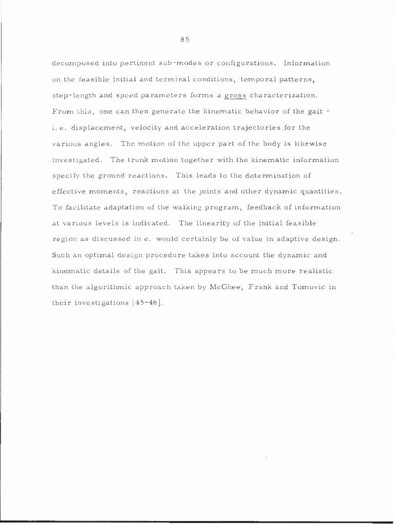
85

decomposed into pertinent sub-modes or configurations. Information

on the feasible initial and terminal conditions, temporal patterns,

step-length and speed parameters forms a gross characterization.

From this, one can then generate the kinematic behavior of the gait -

1. e. displacement, velocity and acceleration trajectories for the

various angles. The motion of the upper part of the body is likewise

investigated. The trunk motion together with the kinematic information

specify the ground reactions. This leads to the determination of

effective moments, reactions at the joints and other dynamic quantities.

To facilitate adaptation of the walking program, feedback of information

at various levels is indicated. The linearity of the initial feasible

region as discussed in e. would certainly be of value in adaptive design.

Such an optimal design procedure takes into account the dynamic and

kinematic details of the gait. This appears to be much more realistic

than the algorithmic approach taken by McGhee, Frank and Tomovic in

their investigations [45-48].

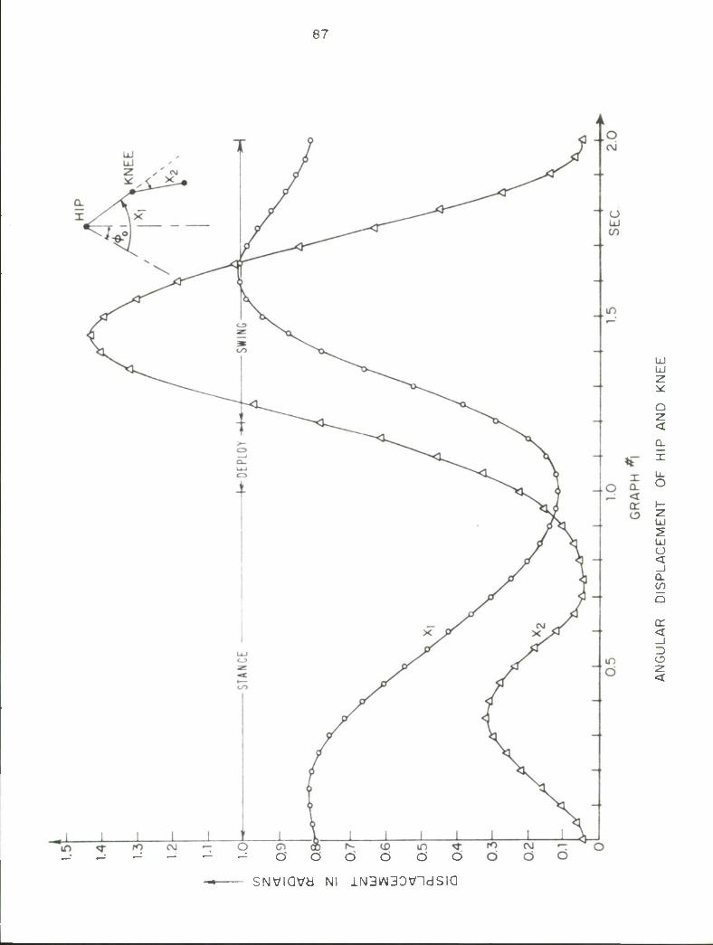
87

UJ UJ

Q

< Q. X

UJ

UJ u «t _J Q. en Q

tr < 3 O

d d d ci o' d SNVIQVH Nl lN3W3DVldSIQ

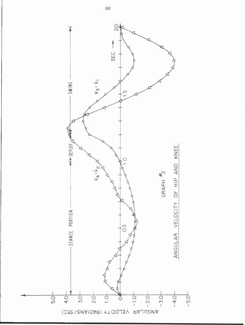
88

(D3S/SNVIQVU) A1I0013A UVinONV

89

O d

o o " o O o in CM a m o in

o o o o in d in CD

, -7 — (Si I I I

m CM

(203S/SNViava) NOII\/U3"13DOV avmoiw

90

r4.0 r-40.0

-3.6

-1.6

H.2

-36.0

3.2 -32.0cT o

,_^ Ul o CO Ul CO \ <

2.8 g -28.0 5 cr CO "-^ z >- " o H H o <

2.4 o -24.0 £T _i Ul Ul _J > Ul

~ o cr (_> < <

2.0 ^ -20.0 cr o < z _i < _ 3

O

-16.0

12.0

GRAPH ^4

ROTATION OF THE FOOT IN DEPLOY PORTION

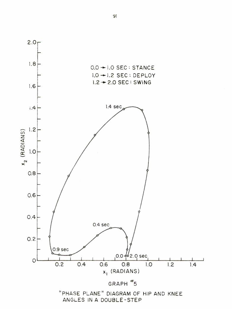
91

2.0r

1.8 -

.6 -

1.4 -

^~. 1.2 in z < Q < 1.0

X

0.8U

0.6-

0.4-

0.2-

0

0.0-^1.0 SEC: STANCE I.0-H.2 SEC: DEPLOY 1.2 — 2.0 SEC: SWING

x, (RADIANS)

GRAPH *5

"PHASE PLANE" DIAGRAM OF HIP AND KNEE ANGLES IN A DOUBLE-STEP

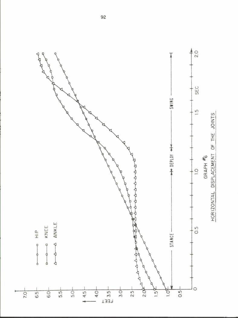
92

oo

x CL < cr o

UJ

UJ o < CL to Q

Z o M

o I

1333

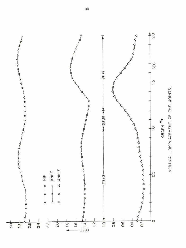
93

LU Ld _J

0- -z. X * <

o S J <3

6 1 i «3

0 1 j <ij

o ao CM

C\i c\i

o

I-

ol

si

X z a. LDI

< s cr UJ| o ^. <t!

_)•

CLi (/> Q;

_J: < (J

K

94

LD z en o »- (- z o o < -5 UJ or UJ

00 X t Q h- X z

3 O 6

or o

or en

< o or

t- or Q UJ Z > <

sai NI S3oaod ~ivDiia3A

95

(/)

O ->

Id

UJ o tr o

o z <

z o I- u < UJ

3 O

o

z o M cr o x

o d

o o o if> d ui ro ro co

O O O O O |£) O iri

o Q If)

o o O iri

I I

o m co ro

O d ro

sai NI s^oaod IVJLNOZIHOH

96

Q-

X

UJ _J

<

? I

o o o O <J> 00 o O o ro CM r

san-iood NI SIN3WOW

CO

o ~3

Lu X (-

t- o <

C CO T h- a. z < LLJ

CL :> O o

s

LU > 1- CJ UJ

o O O O o 1

CO 1

rO l i

U) 1

97

< -z. o

w - <

cc Q2

< ? o

I

> D O < O < cr cc UJ o o cr

<

4 I I

A

SdNriOd-lOOd Nl S1N3I/\I0W

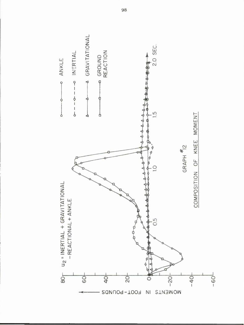
98

z <

o

UJ

< z o <

> < or §3

«l I)

«b A

SQNnOd-lOOd Nl S1N31/MOW

99

40 r

-10

-20

o ° OPTIMAL SOLUTION FROM COMPUTATION

I A INITIAL PROFILE BASED ON APPROPIATE INCREMENT OF GROUND REACTIONS

-25 GRAPH *13

HIP MOMENT FOR VARIOUS PORTIONS (/3) OF GROUND REACTIONS AT DEPLOY

100

20

[ 15

A

-o OPTIMAL PROFILE FROM COMPUTATION

-A INITIAL PROFILE BASED ON APPROPIATE INCREMENT OF GROUND REACTIONS

£ = 1.0

-30

-35

GRAPH *14

KNEE MOMENT FOR VARIOUS PORTIONS (/3) OF GROUND REACTIONS AT DEPLOY

h- ac o Q.

O z B:

o

_j < o

LU

2 o

in cr %~ U.

T to CL Id < rr cr O

CO

z u Q < DC O

O o

>- o O _l 1- CL ce UJ o

|

CL

| o o o o rO CO

I

o o

o o

i

O o in

!

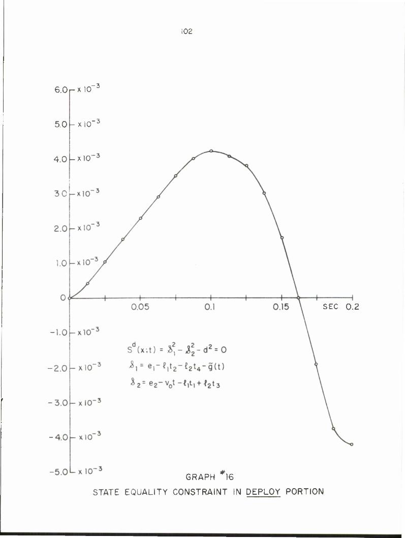
i02

6.0r*10 -3

5.0 - x 10 3

4.0 -xlO

SEC 0.2

GRAPH 16

STATE EQUALITY CONSTRAINT IN DEPLOY PORTION

103

o VI

o 0)

<n o o

+ T3

+ C\J

X

(/) 00

L d

cr O u_

h- z < cr

&£ z 2 r*- O h- *""" o cr

o X . a. CL >-

< to or -1 z o < ^

z> ^ O CD LU Z

LU h- < f- co

104

36 ©

34

32

3ut

DE

GR

EE

S

ro

00

-

5 26 —

o <M

X

UJ"24

CD z < UJ 22 UJ z

< 20 / Sd=^ + X|-d2=0 t-

z iise,-l,t2-l2t4-h(0)

18 — ^2= 62-1,1,+ L2t3

t,= Sin (x,(0)-<£0)

16 t2= Cos(x,(0)-o>0)

t3=Sin(x2(0)-x,(0) + o>0)

14 t4=Cos(x2(0)-x,(0) + c/|))

©/

I? IIII i i I i i i i i i i i i i 8 10 12 14 16 18

INITIAL HIP ANGLE, x^oJ.IN DEGREES

GRAPH *18 THE SET OF INITIAL ANGLES (x^O.x^O)) WHICH SATISFIES THE ENTRY CONDITION

20 22

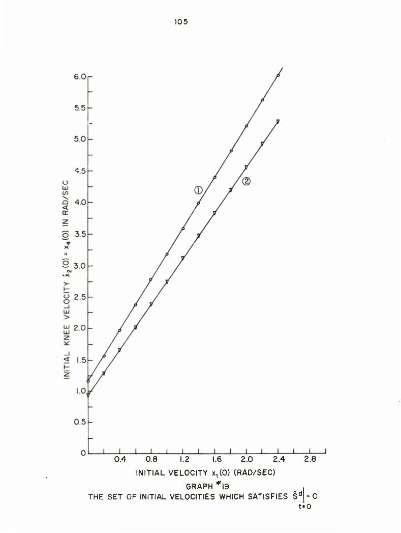
105

0.4 0.8 1.2 1.6 2.0 2.4

INITIAL VELOCITY x^O) (RAD/SEC)

GRAPH #19 . THE SET OF INITIAL VELOCITIES WHICH SATISFIES Sd| = 0

t-0

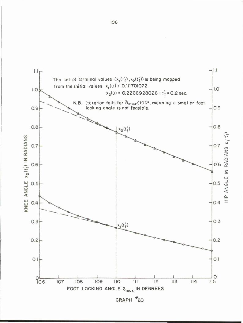
106

1.1

0 106

The set of terminal values (x,(t'f),x2(tf)) is being mapped

from the initial values x,(0) = 0.111701072

x2(0) = 0.2268928028 . t'f = 0.2 sec.

N.B. Iteration fails for SmaX<106o, meaning a smaller foot locking angle is not feasible.

,1.1

1.0

107 108 109 110

FOOT LOCKING ANGLE 8 max

III 112

IN DEGREES

113

H0.6

X

CO

< a < or

UJ _)

< 9- x

0 115

GRAPH 20

107

5.0 r-

0 0.4 0.8 1.2 1.6 2.0 2.4 2.8 TERMINAL HIP VELOCITY x,(t}) s x,(tj) IN RAD/SEC

GRAPH *21

109

F. Conclusions

A new quantitative study of the human locomotion problem has

been developed using the methods of optimal programming and control

theory. The multi-arc formulation is based on the qualitative

properties of the biped gait. Results of the numerical experiment

indicate that the theory is highly relevant and agrees well with experi-

mental results to-date. Because of the flexibility of the method, the

theory can certainly be used to study various types of gait, normal or

pathological. The quantitative method should find importance in

prosthetic design. Eventually, it is hoped, through systematic studies

like the one described, locomotion by programmed stimulation will be

realized.

111

Reft; rences

1 . Bernstein, N. , Popova anci Mogilansky, "Technique of the Study of Movements", Moscow, Gossidat, 1934.

2. Fenn, W. O. , "The Mechanics of Muscular Contraction in Man", J. App. Physio. 9, p. 165 . 1938.

3. Ibid. , "Work Against Gravity and Work Due to Velocity Changes in Running", Am. J. Physiol. , No. 93, p. 433+, 1930.

4. Steindler, A. , "Mechanics of Normal and Pathological Locomotion" (book), Springfield, 111. . Charles C. Thomas, Publisher, 1935.

5. Elftman, H. , "Biomechanics of Muscle", J. of Bone and Joint Surgery, Vol. 48-A No. 2, March, 1966.

b- Ibid. , "The Basic Pattern of Human Locomotion", Annals of New York Acad. Science, No. 51, p. 1207+, 1951.

7. Ibid. , "Skeletal and Muscular Systems: Structure and Function", In Medical Physics (book), p. 1420+, Chicago, Year Book Publishers, 1944.

8. Ibid. , "Forces and Energy Changes in the Leg During Walking", Am. J. Physiol., No. 125, pp. 339-356, 1939.

9. Liberson, W. T. , "Biomechanics of Gait: A Method of Study", Archives of Physical Medicine and Rehabilitation, Jan. , 1965.

10. Wilson, P. D. and Klopsteg, P. E. (Editors). "Human Limbs and Their Substitutes". McGraw-Hill, New York, 1968.

11. Close, J. R. , "Motor Function in the Lower Extremity", American Lecture Series Publication No. 551, Charles C. Thomas, Publisher, Springfield, 111., 1964.

12. College of Engineering, University of California (Berkeley), "Fundamental Studies of Human Locomotion and Other Information Relating to Design of Artificial Limbs", Rep. to National Research Council Artificial Limbs, 1947.

13. Bresler, B. and Frankel, J. P. , "The Forces and Moments in the Leg During Level Walking", Trans, of American Soc. of Mechanical Engineers, p. 27 , Jan., 1950.

14. Crochetierre, W. J. , Vodvnik, L. , Reswick, J. B., "Electrical Stimulation of Skeletal Muscle -A Study of Muscle as an Actuator", Medical and Biological Engineering, Vol. 5, pp. 111-125, 1967.

15. Ibid. , "Control of a Skeletal Joint by Electrical Stimulation of Antagonists", Vol. 5, pp. 97-109, 1967.

112

16. Scott, R. N. , "Myo-electric Control Systems" in S. Levine (Ed. ) "Advances in Biophysics and Fio-engineering" (book), Prentice- Hall, 1969.

17. Milner, M. , Quanbury, A. O. and Edwards, E. P. , "Progress Report No. 1-Human Locomotion by Ordered Electro-Stimulation of the Available Musculature", LTR-CS-6, April, 1969, Control Systems Lab. , National Research Council, Ottawa, Canada.

18. Ibid. , "Progress Report No. 2-Human Locomotion by Ordered Electro-Stimulation of the Available Musculature", LTR-CS-ll, September, 1969. NRC, Ottawa, Canada.

19. Ibid. , "Progress Report No. 3-Analysis of Footswitch Data in Walking", LTR-CS-26, January, 1970, NRC, Ottawa, Canada.

20. Ibid. , "Progress Report No. 4-Analysis of Muscle Activities at Various Speeds and Pace Periods from EMG's with Indwelling Electrodes", LTR-CS-33, June 1970, NRC, Ottawa, Canada.

21. Mountcastle, V. B. (Editor), "Medical Physiology" (book), Vol. 2, C. V. Mosby, St. Louis, 1968.

22. Vukobratovic. M. , Juricic\ D. , "Contribution to the Synthesis Biped Gait", IEEE Trans, on Bio-Medical Engineering, Vol. BME-16 No. 1. January. 1969.

23. Vukobratovic. M. , Frank, A. A. , Juricic D. , "On the Stability of Biped Locomotion", IEEE Trans, on Bio-Medical Engineering. Vol. BME-17, No. 1, January, 1970.

24. Tomovic, R. . "Outline of a Control Theory of Prosthetics", IFAC Proceedings, Basle, Switzerland, 1963,

25. Ralston, H. J. , "Energy-Speed Relations and Optimal Speed During Level Walking", Int. S. Augew. Physiol. einschl Arbeitsphysio. Bd. 17, 277-283, 1958.

26. Cotes, J. E. , and Meade, F. , "The Energy Expenditure and Mechanical Energy Demand in Walking", Ergonomics, April, I960.

27. Nubar, Y. and Contini, R. , "A Minimal Principle in Bio-Mechanics", Bull. Math. Biophysics, No. 23, pp. 377-390. 1961.

28. Beckett, R. and Chang, K. , "An Evaluation of the Kinematics of Gait by Minimum Energy", T. of Biomechanics, Vol. I, pp. 147-159, 1968.

29. Vukobratovic, M. , Marie, M. and Garvilovic, M. , "An Approach to the Synthesis of Lower-Extremity Control", Proc. 2nd Inter- national Symp. on External Control of Human Extremities, Yugoslav Committee for Electronics (ETAN), Belgrade, pp. 206-211, 1967.

113

30. Hill, J. C. , "A Model of the Human Postural Control System", 8th-IEEE Symp. on Adaptive Processes; Decision and Control, December, 1969.

31. Inman, V. T. , "Human Locomotion", Canadian Medical Assoc. J. , Vol. 94, pp. 1047-1054, 1966.

32. Lissner, H. R. and Williams, W. , "Biomechanics of Human Motion" (book), W.B.Sanders, Philadelphia, Penn. . 1962.

33. Ciliana, H. L. , "Modelling the Human Leg in Walking", M. Eng. Thesis, McGill Univ. , Montreal, Quebec, Canada, August, 1968.

34. Wallach, J. and Saibel, E. , "Control Mechanism Performance Criterion for an Above-Knee Leg Prosthesis", J. of Biomechanics. Vol. 3, pp. 87-97, 1970.

35. Lasdon, L. S. , Waren, A.D. and Rice, R.K. , "An Interior Penalty for Inequality Constrained Optimal Control Problems', IEEE Trans, on Automatic Control, Vol. AC-12, No. 4, August, 1967.

36. Wilkie, D. R. , "Facts and Theories about Muscle", Prog, in Biophysics and Biophysical Chemistry, No. 4, p. 288 + , 1954.

37. Ibid. , "The Relation between Force and Velocity in Human Muscle ', J. Physiol. , No. 110, p. 249+, 1950.

38. Vickers, W. , "A Physiologically Based Model of Neuromuscular System Dynamics", IEEE Trans, on Man-Machine Systems, Vol. MMS-9, No. 2, p. 21+, 1968.

39. McRuer, D. et al, "A Neuromuscular Actuation System Model", IEEE Trans, on Man-Machine Systems, Vol. MMS-9, No. 3, p. 61+, 1968.

40. Bigland, B. and Lippold, O. C. J. , "The Relation between Force, Velocity and Integrated Electrical Activity in Human Muscle", J. Physiol. , No. 123, p. 214 + , 1954.

41. Stark, L. , "Neurological Control Systems-Studies in Bioengineering" (book). Plenum Press, N. Y. , 1968^ (p. 302+).

42. Houk, J. , "A Mathematical Model of the Stretch Reflex in Human Muscle Systems", M. S. Thesis, M. I. T. , 1963. (Also appears in "The Application of Control Theory to Physiological Systems" book by T. Milhorn, Saunders, 1963, Chapter 17.

43. Bryson, A.E. and Ho, Y. C. , "Applied Optional Control: Optimization, Estimation and Control" (book), Blaisdell Publishing Company, Waltham, Mass. , 1968.

114

44. Lele, M. M. and Jacobson, D. H. , "A Proof of the Convergence of the Kelley-Bryson Penalty Function Technique for State-Constrained Control Problems", J. Math. Anal. Appl. . 1969.

45. McGhee, R. B. , "Some Finite State Aspects of Legged Locomotion", Math. Biosciences, Vol. 2, No. 2, pp. 67-84, 1968.

46. McGhee, R. B. and Frank, A. A. , "On the Stability Properties of Quadruped Creeping Gaits". Math. Biosciences, Dec. , 1968.

47. Tomovic.R. and McGhee, R. B. , "A Finite State Approach to the Synthesis of Bioengineering Control Systems", IEEE Trans, on Human Factors in Electronics, Vol. HFE-7, No. 2, June, 1966.

48. Tomovic, R. , "Multi-level Control of Mechanical Multivariable Systems as Applied to Prosthetics", IEEE Trans. Automatic Control (short papers), Vol. AC-13, February, 1968.

.1 Diroclnr/ltoa-ar,), |Rm )C12B| ice ollh-Secretary ol Del.-.,.. nagon •hinetoo, D C 20101

Toclmir.l l.,br«rV DDK and t Boom 1C-122, The Pantigoi Waah.ngton, D C £0101

H„r . 1[JI I Thf Ptnlif w... in(t« D C 20301

Rich .-1 J GBWM

••( EltJI kc»4« my.

Difc i« Do mil tailor. C»

iron si A,r ,...,.., V,, "*• Z" „. RMM ,.... (STEPD-SD(S)I S, ,r Ur,. •1 i>. I (i

e'Circle Dmif.li . Hi h itin

M> H. E Webb Jr (EMF ».;: A,, D t.,-„, Ce Irr

Ciiin.il Intcllij • AUnL CRS/ADD/PUBLICATIt w...hn,,:ii.ii. i> C it^o1'

M< H it Loch

USAF Security S K-lly An Font

AMSEL-SC Cry.lal Producll D

OC-DD 8888 F«ll>o» Avenue. P. 0. Box ZJ017

xl" DT San Diego, California, 9ZIZJ

BL-FM-P CT-D CT-B

CT-O McAfc. Wa.h„,gton, D C. 20Jli

CT-I CT-A NI.-D |D, II Br

Nl ( (ECACJ, Ann: ACOAT North Stvcrn

: STEWS RE-1 : ,-. • Sand• Miaailc H-nh

Molico BKPD2

U5AK European Otll.r al A,,, APO, Ne» York 091.67

J S Array S*i Ittn: 1AHD-T arllnilon lull S

Kl.-S Kl SM Kl i

.1 Di Engineering and Applied

>r*ily ofV.rg.ma lolleaville, Virginia iiioi

•clriealEngtM

( nidi no

ring and Appt.rd Phytii

H.ii

Hl( USAF (AfMDSn) Thf Prnlagun Wiili.n,l.r, D C £01!

Commanding Offae

inglon, D. C. 20J90

'i"I Commander (ADI.|

John.v.He, W.trmin Atln: NADC Librar

P O Bo, Lo, An!.)

I' Camp.. Ji ACUA/U1 190) I'ion.ylv,,,,. AvtnV Wa.lnr.,1...., D C 2Qasi

LI Cnl H W Ja.

Ho.AF5C [SGGP)

Naval Sacurlly Group Cor Naval Security Group l[*a ,Atir: G4)

r.i. uatr- A. • Ml Ti.al lah„r.io

i.' •

orma In E. Cab

111 r o( T» '" Pa i dan*, C 1.1, "'* " '"' Thr John. Hop,, , H. • m

C.j.gu Slh r Sp.mg M • •.;..• i £0910

MIT 1.1,i.

P Cl it.

•anal, SMUPAHT-S

xii G w D.,,.. tor

Mobility Equlpmi nl Ht man) 1 . ,,[,.,•

•

Virginia 22060 Am"/ *' Waatangl

Offlcai (AMSF! r-i.-w

Mia tit* Range

S-R1

.Naval Shi

'-•

Allni Library San Diego, California

(.-.•

1 i

ref. C*liloroia

HEX 0), Im 2"ilJ Mam Navy Hldg B)T' ""he Navy

• • •

Air Force Aviomc. Laborai

(S M: FA-A

PhiU c iph

Re 1. m.S • •

u s Am V S Naval O.dnancr Lai

: . •

AFALIAVIA/H II Url

Dlractoi M Pacully Hr.rarih D,.pl ntlha A,, r U. S. Air Force Academy Colorado Spring., Colorado long

• • ....

U S Poat OHi.r Dtpi

.AM'-n (SMTAE/LI He!

. Di. , CIS Oepl. Uia

naied Scienet Latwra ,,ly ol lihnma

, lllmoia 61B01

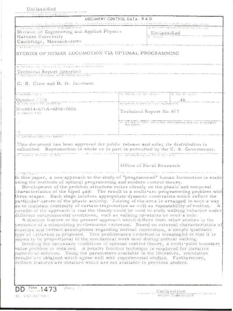
Unclassified S1-.unt> Cl.issifu atu'ii

DOCUMENT CONTROL DATA R&D ,; „••. tract >in.] uittvxm,) .-,< >•>!,,ii.-n ..•<,.•.< '•< Ltitvrvd wltor, tin •r.tll rrfiort i s

i OH '. •, r, A 11 NO AC T 1 v i r Y (Corporate authori

Division of Engineering and Applied Physics Harvard University Cambridge, Massachusetts

:o. hi PORT SECumiy c L A -

Unclassified W< RHOUP

< R 1. P O R T T I i I F.

STUDIES OF HUMAN LOCOMOTION VIA OPTIMAL PROGRAMMING

4. OESCRif'1 i v b" f\ O . t. -;<,-• -' r-•>-"•" ' <'"'' 'm 'tj;j l'e dales,)

Technical Report (Interim) _ '•> AU [tiORiSi <h~irst nt*me, middle initial, l/i^i ii,>nw,

C. K. Chow and D. H. Jacobson

6 RfPOR: "Ait

CO^,^(<AC^ OK oRANT NO

N-00014-67-A-0298-0006 b. r KOJ E L. T NO

'a. TOTAL ,JO OF PAGE • /K NO OF- RE F S

48 in. ONlGiru lOR'b Rb-.POKT NUWPfKISI

Technical Report No. 617

*£<. OTHER REPORT NO(S> (Any othrr numbers that may /><• assigned it,is report)

10 DISTRIBUTION STATEMENT

This document has been approved for public release and sale; its distribution is unlimited. Reproduction in whole or in part is permitted by the U. S. Government. 11 SUPPLE IFflTflR^ NOTES I. iPk^JSuH.;iu MIL.ITAKV ACTIVITY

Office of Naval Research

[n this paper, a new approach to the study of "programmed" human locomotion is made using the methods of optimal programming and modern control theory.

Development of the problem structure relies closely on the phasic and temporal characteristics of the biped gait. The result is a multi-arc programming problem witl three stages. Each stage involves appropriate dynamic constraints which reflect the particular nature of the phasic activity. Joining of the arcs is arranged in such a way as to maintain continuity of certain trajectories as well as repeatability of motion. A novelty of the approach is that the theory could be used to study walking behavior under different environmental conditions, such as walking up-stairs or over a hole.

A distinct feature of the present approach which differs from other studies is the presence of a minimizing performance criterion. Based on external characteristics of muscles and certain assumptions regarding normal locomotion, a simple quadratic type of criterion is proposed. This performance criterion is meaningful in that it is shown to be proportional to the mechanical work done during normal walking.

Invoking the necessary conditions of optimal control theory, a multi-point boundary value problem is obtained. A penalty function technique is employed for iterative numerical solution. Using the parameters available in the literature, simulation results are obtained which agree well with experimental studies. Furthermore, refined features are obtained which are not available in previous studies.

DD FORM 1473 (PAGh

S/I4 0 10 1 • 807

Unclassified Security Classification

Unclassified Security Classification

KEv rtOROS LINK A

Biped Locomotion Optimal Programming Human Locomotion Bio-Medical Engineering Mathematical Biosciences Mathematical Modelling Simulation

I S

DD FORM i NOv es 1473 (BACK Unclassified

S / N 0t01-807-sa?1 Security Classification