towards modeling texture in symbolic data · towards modeling texture in symbolic data mathieu...

TOWARDS MODELING TEXTURE IN SYMBOLIC DATA

Mathieu GiraudLIFL, CNRS

Univ. Lille 1, Lille 3

Florence LeveMIS, UPJV, AmiensLIFL, Univ. Lille 1

Florent MercierUniv. Lille 1

Marc RigaudiereUniv. Lorraine

Donatien ThorezUniv. Lille 1

{mathieu, florence, florent, marc, donatien}@algomus.fr

ABSTRACT

Studying texture is a part of many musicological analy-ses. The change of texture plays an important role in thecognition of musical structures. Texture is a feature com-monly used to analyze musical audio data, but it is rarelytaken into account in symbolic studies. We propose to for-malize the texture in classical Western instrumental musicas melody and accompaniment layers, and provide an al-gorithm able to detect homorhythmic layers in polyphonicdata where voices are not separated. We present an evalua-tion of these methods for parallel motions against a groundtruth analysis of ten instrumental pieces, including the firstmovements of the six quatuors op. 33 by Haydn.

1. INTRODUCTION

1.1 Musical Texture

According to Grove Music Online, texture refers to thesound aspects of a musical structure. One usually differen-tiates homophonic textures (rhythmically similar parts) andpolyphonic textures (different layers, for example melodywith accompaniment or countrapuntal parts). Some moreprecise categorizations have been proposed, for exampleby Rowell [17, p. 158 – 161] who proposes eight “texturalvalues”: orientation (vertical / horizontal), tangle (inter-weaving of melodies), figuration (organization of music inpatterns), focus vs. interplay, economy vs. saturation, thinvs. dense, smooth vs. rough, and simple vs. complex. Whatis often interesting for the musical discourse is the changeof texture: J. Dunsby, recalling the natural tendency to con-sider a great number of categories, asserts that “one hasnothing much to say at all about texture as such, since alldepends on what is being compared with what” [5].

Orchestral texture. The term texture is used to describe or-chestration, that is the way musical material is layed out ondifferent instruments or sections, taking into account regis-ters and timbres. In his 1955 Orchestration book, W. Pistonpresents seven types of texture: orchestral unison, melodyand accompaniment, secondary melody, part writing, con-trapuntal texture, chords, and complex textures [15].

c© Mathieu Giraud, Florence Leve, Florent Mercier, MarcRigaudiere, Donatien Thorez. Licensed under a Creative Commons At-tribution 4.0 International License (CC BY 4.0). Attribution: Math-ieu Giraud, Florence Leve, Florent Mercier, Marc Rigaudiere, DonatienThorez. “Towards modeling texture in symbolic data”, 15th InternationalSociety for Music Information Retrieval Conference, 2014.

In 1960, Q. R. Nordgren [13] asks: “Is it possible tomeasure texture?”. He proposes to quantify the horizontaland vertical relationships of sounds making up the texturebeyond the usual homophonic/polyphonic or light/heavycategories. He considers eight features, giving them nu-merical values: the number of instruments, their range,their register and their spacing, the proportion and reg-ister of gap, and doubling concentrations with their reg-ister. He then analyzes eight symphonies by Beethoven,Mendelssohn, Schumann and Brahms with these criteria,finding characteristic differences between those composers.

Non-orchestral texture. However, the term texture also re-lates to music produced by a smaller group of instruments,even of same timbre (such as a string quartet), or to mu-sic produced by a unique polyphonic instrument such asthe piano or the guitar. As an extreme point of view, onecan consider texture on a monophonic instrument: a sim-ple monophonic sequence of notes can sound as a melody,but also can figure accompaniment patterns such as arpeg-giated chords or Alberti bass.

Texture in musical analysis. Studying texture is a partof any analysis, even if texture often does not make senseon its own. As stated by J. Levy, “although it cannot ex-ist independently, texture can make the functional and signrelationships created by the other variables more evidentand fully effective” [10]. Texture plays a significant rolein the cognition of musical structures. J. Dunsby attributestwo main roles to texture: the illusion it creates and theexpectation it arouses from the listeners towards familiartextures [5]. J. Levy shows with many examples how tex-ture can be a sign in Classic and Early Romantic music,describing the role of accompaniment patterns, solos andunison to raise the attention of the listener before impor-tant structural changes [10].

1.2 Texture and Music Information Retrieval

Texture was often not as deeply analyzed and formalizedas other parameters (especially melody or harmony). Inthe field of Music Information Retrieval (MIR), the notionof texture is often used in audio analysis, reduced to tim-bral description. Any method dealing with audio signals issomewhat dealing with timbre and texture [3, 9]. Based onaudio texture, there were for example studies on segmenta-tion. More generally, the term “sound texture” can be usedto describe or synthesize non-instrumental audio signals,such as ambient sounds [18, 19].

15th International Society for Music Information Retrieval Conference (ISMIR 2014)

59

Among the studies analyzing scores represented by sym-bolic data, few of them take texture into account. In 1989,D. Huron [7] explains that the three common meaningsabout the texture term are the volume, the diversity of el-ements used and the “surface” description, the first twobeing more easily formalizable. Using a two-dimensionalspace based on onset synchronization and similar pitch mo-tion, he was able to capture four broad categories of tex-tures: monophony, homophony, polyphony and heteropho-ny. He found also that different musical genres occupy adifferent region of the defined space.

Some of the features of the jSymbolic library, used forclassification of MIDI files, concern musical texture [11,12]. “[They] relate specifically to the number of indepen-dent voices in a piece and how these voices relate to oneanother.” [11, p. 209]. The features are computed on MIDIfiles where voices are separated, and include statistical fea-tures on choral or orchestral music organization: maxi-mum, average and variability of the number of notes, vari-ability between features of individual voices (number ofnotes, duration, dynamics, melodic leaps, range), featuresof the loudest voice, highest and lowest line, simultane-ity, voice overlap, parallel motion and pitch separation be-tween voices.

More recently, Tenkanen and Gualda [20] detect articu-lative boundaries in a musical piece using six features in-cluding pitch-class sets and onset density ratios. D. Rafai-lidis and his colleagues segment the score in several textu-ral streams, based on pitch and time proximity rules [2,16].

1.3 Contents

As we saw above, there are not many studies on modelingor automatic analysis of texture. Even if describing musicaltexture could be done on a local level of a score, it requiressome high-level musical understanding. We thus think thatit is a natural challenge, both for music modeling and forMIR studies.

In this paper, we propose some steps towards the mod-eling and the computational analysis of texture in West-ern classical instrumental music. We choose here not totake into account orchestration parameters, but to focus ontextural features given by local note configurations, takinginto account the way these may be split into several lay-ers. For the same reason, we do not look at harmony or atmotives, phrases, or pattern large-scale repetition.

The following section presents a formal modeling of thetexture and a ground truth analysis of first movements often string quartets. Then we propose an algorithm discov-ering texture elements in polyphonic scores where voicesare not separated, and finally we present an evaluation ofthis algorithm and a discussion on the results.

2. FORMALIZATION OF TEXTURE

2.1 Modeling Texture as Layers

We choose to model the texture, by grouping notes into setsof “layers”, also called “streams”, sounding as a whole

grouped by perceptual characteristics. Auditory stream seg-regation was introduced by Bregman, who studied manyparameters influencing this segregation [1]. Focusing onthe information contained on a symbolic score, notes canbe grouped in such layers using perceptual rules [4, 16].The number of layers is not directly the number of ac-tual (monophonic) voices played by the instruments. Forinstance, in a string quartet where all instruments are play-ing, there can be as few as only one perceived layer, severalvoices blending in homorhythmy. On the contrary, somefigured patterns in a unique voice can be perceived as sev-eral layers, as in a Alberti bass.

More precisely, we model the texture in layers accord-ing to two complementary views. First, we consider twomain roles for the layers, that is how they are perceived bythe listeners: melodic (mel) layers (dominated by contigu-ous pitch motion), and accompaniment (acc) layers (dom-inated by harmony and/or rhythm). Second, we describehow each layer is composed.

• A melodic layer can be either a monophonic voice(solo), or two or more monophonic voices in ho-morhythmy (h), or within a tighter relation, such as(from most generic to most similar) parallel motion(p), octave (o) or unison (u) doubling. The h/p/o/urelations do not need to be exact: for example, a par-allel motion can be partly in thirds, partly in sixths,and include some foreign notes (see Figure 1).

• An accompaniment layer can also be described byh/p/o/u relations, but it is often worth focusing on itsrhythmic component: for example, such a layer cancontain sustained, sparse or repeated chords, Albertibass, pedal notes, or syncopation.

The usual texture categories can then be described as:

• mel/acc – the usual accompanied melody;

• mel/mel – two independent melodies (counterpoint,imitation...);

• mel – one melody (either solo, or several voices inh/p/o/u relation), no accompaniment;

• acc – only accompaniment, when there is no notice-able melody that can be heard (as in some transitionsfor example).

The formalism also enables to describe more layers,such as mel/mel/mel/mel, acc/acc, or mel/acc/acc.

Limitations. This modeling of texture is often ambigu-ous, and has limitations. The distinction between melodyand accompaniment is questionable. Some melodies cancontain repeated notes, arpeggiated motives, and stronglyimply some harmony. Limiting the role of the accompani-ment to harmony and rhythm is also over-simplified. More-over, some textural gestures are not modeled here, such asupwards or downwards scales. Finally, what Piston calls“complex textures” (and what is perhaps the most inter-esting), interleaving different layers [15, p. 405], can not


60

::: ./texture -T truth/sonata-quartet.truth --polyphonic data/Mozart-K157-4.krn --score --no-analysisdefault_files= '': ['../../../sonata/data/Beethoven-19-1.krn'], 'bla': ['data/file1.krn', 'data/file2-*.krn']:: 2014-07-19 11:01:49.599179

<Truth 'truth/sonata-quartet.truth'>

Mozart-K157-4==== Mozart-K157-4 - Mozart String Quartet n°4, K 157 ==== C Major, sonata form, 4 voices (SATB): h: homorythmy>>> texture * 1, 75 : mel/acc (SAp / TB) * 8, 82 : mel/acc (SA / TBp) * 9, 83 : mel/acc (SAp / T syncopation, B) * 13, 87 : mel/acc (SAp / TB imitation) * 19, 93 : mel/acc (SAo / TBh) * 20, 94 : mel/acc (SAp / TBhr) * 21, 95 : IMITATION/acc (SA / TB) * 25, 99 : IMITATION/acc (SA / TB) * 102 : mel/acc (S / ATB) * 29, 103 : mel/acc (S / ATBhr) * 30 : mel/acc (S / ATBh) * 104 : mel/acc (SAh/ TBh) * 31, 105 : mel/acc (S / ATBh SPARSE CHORDS) * 33, 107 : acc/mel/acc (S / ATp / B) * 35, 109 : acc/mel (SAT / B) * 36, 110 : acc/mel (SA / TBp) * 37 : mel/acc (SAp / TBp) * 111 : mel/acc (S / ATh, B) * 38, 112 : mel (S) * 39, 113 : acc/mel (ST / ABp) * 41, 115 : mel/acc (S / ATB) * 42, 116 : mel/acc (S / ATBh SPARSE CHORDS) * 46, 120 : homorhythmy (SATop, B) * 49, 120 : mel/acc (SAp / TB) * 124 : mel/acc (STh / AB) * 53 : mel/acc (S / ATBh SPARSE CHORDS) * 63 : acc/mel/acc (S / ATh / B) * 67 : acc/mel (SA / TBh) * 70 : intensification (?)::::::::::::::::::::::::::::::::::::::::::::::::::::::::::::::::::::::::::::::::::::::::::::::::::::::::::::::::

!

"#""

"!

""""

$"$$

"

"

""

" "%""

""

""

"" "

""&&

&&

"

""

"

"

""

""

""

"

mel/acc(SAp / TB)

!!

"#

"

"

""

"

""

"

"

"%""

""

"

"%""

"' ""

"(

"

"

" """"

"

')'

"

""

" "*'+

)

"

""

" ",""

"

"

"

""

"

"""

"

""

"

""

!

!

"%%

"

"-$""

$$

"""

"

""

""

""

".

mel/acc(SAp / TB imitation)!!"

,

" "$$(

(

""

"

"& "

"

""" (

"""

""

"

"(

"""

"

""

"

""

" "

""

" "

""%

""

"

""

"

"$"

""

""

"$

"

."

""

"""""

"

,,""

!

("

"""

""""

mel/acc(SAp / T syncopation, B)!

"

""

"

)7

)+*

"",

"& ""

$$

"""

""."

mel/acc(SA / TBp) "

""

""

,

"""

""

"

- "

""

""

!!

"

$$""

""

""

"""

((

""

"

""""(("

! !

"

"

"

"."

!"""""$

""""

!!

"""

"

""

$

"

"

"

"

""

"

"%"

"&

"

"

"

"."

"

"

"

""

"

"""

$

""" "

""

"""

.

"

""

" """"

. $

"""

! ""."

(

""

""

""""

"""

""

""

"

"

"

"

"

!

!mel/acc

(SAo / TBh)

""

"""

""

"""

"

" """

"

"

"""

"

."

""

+))

14

*

"

"

&

"%"

"

"

"

""

""

""$"

"

" "

" "

""

"

"

""

"

"

"$

"

""

"

"

".

" "

""""

"

"""

""

"

"

"

""

"

""

" "

""

$""" "

"""" "

"

","

-

"$"

"

"

"%

$""

"$

" "

" "

$

!

- " "

"%"

!

!

"("- "

" "

"

"""

IMITATION/acc(SA / TB)!

" "

"

"

"

"

"

$"$

!%

/

""

IMITATION/acc(SA / TB)$

$"$"

"

," "

"

"$" "

%""""

mel/acc(SAp / TBhr)20

))+*

% ""

""

""""" "

$"""

""""

"

"

-

"

%

"""

"

" "

"%

$"

"

""" "

"

"" "

""

"

"

$

!" "- " "

$

- "

%

"""!

"("- "

"

%"

! " "

$

!"

" " " "

"!

!

"%!

"

""

""%

"

$$$$

"

mel/acc(S / ATBhr)

" ""&""""

"

""

"

"""

"

"

%

""

" "

""""

mel/acc(S / ATBh)

"

"""

"

""

-

" " "

"

" "

"

"

"

$

!-

"""

""

-

26

))+*

-

"

""

"""

" "

"

"

"

"""

!

" "

"

"

- ""

$"$

!

" "- "- "

%

"""!

" ""&"

$

"

"- "

"

""

"""

"..

""

acc/mel(SA / TBp)

""

""

.

"%

"

%

".

"-"

%

""

"

$

-

acc/mel(SAT / B)

"

""

""

""

"..

acc/mel/acc(S / ATp / B)

"""

#

"

#

-"" "

""""

"

"

""-

0""

$""

%

""

"

""."

-

"""

"

$$$

"" "

*+))

31

mel/acc(S / ATBh SPARSE CHORDS)

"0

"

""

"-

$$$

"

"

$$$

""

-".

"%

"""

""

"

""

"-""

"

""

"

"

"

"

"

"

"

"

%

$$

"$ -"

"" "- ".%

%" "

"""

-

acc/mel(ST / ABp)

"""

%

"

"

-

"

"%

"-%. ""

""

0

"

" """

%

-

"

"

0

"

""

"

"

""""

""

"

"

"

"

""

"

!

!

"

,,,"""

$$$

-

"""

"

""

mel (S)

""

"

"" "

""

""$""""

$$$"

$$$""

-

""

"

-""

* "

mel/acc(SAp / TBp)

37

))+

"%"

""

$$ "

"

"""

"!!

&&

"""

"

""""

"

"!

mel/acc(S / ATB)

"""

""

"


"""

"

"

-

"

"

" "

"%"

""

"

"

""%"

mel/acc(SAp / TB)"

"

"

"

"%"

"

"

--

"

""

"

"

"""

"

""

""""

-

"""

"

"""

"

"%

"

"

%

%%

#

"-

"

"

"

"

"%

%%#

"

"

"

"

"

"

"

"

"

"

"%-

" "$$

" "

""

"

" " "

"

"$

" "

"%""

" "$$$*

+))

44

"

""

-

" "$$$

" "

""

" "--

"

"""

"

""

"

""

"

"""

"

""""

homorhythmy(SATop, B)

" "- "

""

"

"""

"

"

""

"" "

,,,

" " " " "

"""

" "$$$

" "

"""

" "

$$$

" "

"""

" "

,,,-

" "

$$$

" " " " "" "

"""

"" "$$$

"

"

""

"$$$

"""

"""

mel/acc(S / ATBh SPARSE CHORDS)"

"""

" "$

"$$$

""

"""

52

))+*

"""""""

$$$$

"""""""

""" " " " "" "

,,,

" " "$$$

"

"""

""

$$

" "

"

" "$$$

""

""

""""

"

"""" .

."

"""""""

"

""

"

$

"

$$

"$

$$

$

"-"..

"acc/mel/acc

(S / ATh / B)

$""

#

"

""""

""""""" "-" "

"""

"

""

"

""" "$$$

"

$$$

"""

"

""

"

"- - "

"$

"

""

#

"""

""

"".

."

"- "

"""

59

))

*+

"

""

$

".

"""

""

""

"" 0 "

"$

"-

"- "

"""

"""

"

$ "..

""

""

.

"" ""

""$$

"

#

"

"

"

intensification(?)#

""

"

"""

""

"""

1

"

"

""

"""

"

acc/mel (SA / TBh)

""

%

"""""

- ." %""

".

""

""

"

""

" """

""

"""( "

"

"

"

"

"

&""""

""

""

"

"

"""

"""

"

"

"

"

""

"" "

."

"

".

" ""

."""

(

"

"

"

"

"

"."

"

"""

""

(

"

"

""

" "

"(

"+*

"66

))

"

"."

"

"

"""

"""0

%

""""

""-

""""

"" -0

%

"" "

"""

""

%

.

."

%"%

%

""

1

""

"$"

"

"

"

"

"

"""%""

"

"

"

" """"

"

"

" "

"

"

"

""

""""

"

" "

"

"

""

""

"

. "!!

"#"

""

"

&&

"

"""

"

"

"

"

""

"""

$"$$

"

"

" """"

"

""

"

"

"

" "

"

". .

"

"

"

""

"

""

" "

" """

"

"

"* "

72

))+ &

"

"

" """"

.

"""

"

$$$" "

"-

,,,"

""""

"" "

&

""""

.&&

"

""

"

!mel/acc

(SAp / TB)

"#""""!

0

""

!

"

,,""

""""

mel/acc(SAp / T syncopation, B)

(

!

""""

"

""."

mel/acc(SA / TBp)

"",

" "

""

"

$$

"""

& ""

""

,

"

""

"

"""

$$"- "

""

"

"

""

"

""

"""

((

(

""""(

""""

"

"

%%"

!

!"

$$"

$

"

"

( "

""- " ""

""

"

78

))+*

""%

""""

""

"

""

" "

"

"

"",

""

""%"

"

" ""

""%"

""

"

"

"""

""

"

""

"

"""

"

"""

(" ("$$

"

mel/acc(SAp / TB imitation)

."

""

"""

"

""

,

""

"

$" ""

"

"

"

""

"

"

"

"

"

"

""

((

"

""

" "

"

"""

" "

""

"$

"""

!!

."

" ""

"

.

""

"

""

.

""

""

!!

"$

" $"

""

"

""

""

"

""

"".""

"""

$

"""""

"""

"""

!!

""""

""

$""""

""

$

""

*+))

85

"""

("""

""

"""

""

""

!&

"

"""

""

!

"

" ""

"

"

"

""

."

"

$""

"

"

"

"

"

!

!

"

"

"

&"."

"

"

"

"

"

"

"."

""

"%"

""

"$

""

""

"

"%"

""

"" "

"

"

-"

"

"

"

""

"

"

"

""

""

"

"""

"$"

"

"

""""

%

""

"""

""""

""

"

"

""1

" "

"

"

"

"

"

."

"""

$"$$

"""/

%

"""

"

"

"

""

1IMITATION/acc(SA / TB)

"-""

""

"""

"

!

!mel/acc

(SAo / TBh)

" """

"

""

"

"

"

"""

"

""

"

" "

"

&+))

92 "

* "%"

""

"

"

"

""

"

"

"

"

"

"

"

"

"

"

"""

"

"%"

"

"

"

"

"

"

mel/acc(SAp / TBhr)

""%%

" "

"""

"""" "

""$

""""

mel/acc(S / ATBhr)

"

(

""

!"""%

"""

$

"" ""

"""

"""

-""

"""

%

"""

""""

""

!

!

"""

""!

$"

"""

"

"" !$"

"

"

"

""

"""mel/acc

(S / ATB)

""%

"""

&" ""

!"""

%

""

"

$

""""!"

""" ""

!

$

"

" "

"

"

""+

)

*

99

IMITATION/acc(SA / TB)

)

!

$

"$"

("""

!

"""

"!

$

"$

" "

"

"

""

!

"""

"

"

"

""""

("!

$

!""%

"

"!

!

"%"

"

"

"""

.

"""

"""

$$$"" "

"

"

.

.""

"

""

"""

"" "$$$

#

"""

acc/mel/acc(S / ATp / B)

"

""

""

"

""""

""

""

""

"""

"".

""" $

$$"""

"""


$$$"$

$$$

"

"""

%

0""

"

acc/mel(SA / TBp)%

"-"."%

"""

0 """"

""

*+

mel/acc(SAh/ TBh)

104

))

%

""

%". "

""

""""

"

.

."" "

""""

""

$"""

#

""

"

acc/mel(SAT / B)

"""

%

""

"-"

"

"" "

"

$

"

""""

"$$$

" " "

"""

" "$$$"

""""

"""""

"

""

""

""""

mel/acc(S / ATBh SPARSE CHORDS)"

"""

"

"""

"

""" """

!

!!""

" "

""

&

"

&

" "

$$$

"""

"""

"""

-

" " " %

"""

acc/mel(ST / ABp)

%"

"

"

""

"%. "- ""

"

""

"

mel (S)

*+))

111mel/acc

(S / ATh, B)

""

" ",,,$

$$""

"""

"

""

%"

"

"

" "

""

"

"

"

"

"""

mel/acc(S / ATB)

!%

"""0

"""

"

"

0 "%. ""

"""

"""

"

""

"

"

"%""

"

"

"

"""

"

"

"

"

" """"

"""

""" """" "

"

"""

"

"

"

"

"

""""

""

"""""

%"

"

"

%%%

#

mel/acc(STh / AB)

"%"

"

"

"

#

%%%

"

" "

""

"

" "$$$

" "

"%"

"" "

$$$

"

"""

118

))+*

""

"

" "

""

"$$$"" "

"""

""%"

""""

"

"%"

"

"

"

""" $

$$$

"

""

" "

"

"

" "

"""

mel/acc(SAp / TB)

"

1, 75 : mel/acc (SAp / TB)8, 82 : mel/acc (SA / TBp)9, 83 : mel/acc (SAp / T syncopation, B)

13, 87 : mel/acc (SAp / TB imitation)19, 93 : mel/acc (SAo / TBh)20, 94 : mel/acc (SAp / TBhr)21, 95 : imitation/acc (SA / TB)25, 99 : imitation/acc (SA / TB)

102 : mel/acc (S / ATB)29, 103 : mel/acc (S / ATBhr)30 : mel/acc (S / ATBh)

104 : mel/acc (SAh/ TBh)31, 105 : mel/acc (S / ATBh sparse chords)33, 107 : acc/mel/acc (S / ATp / B)...

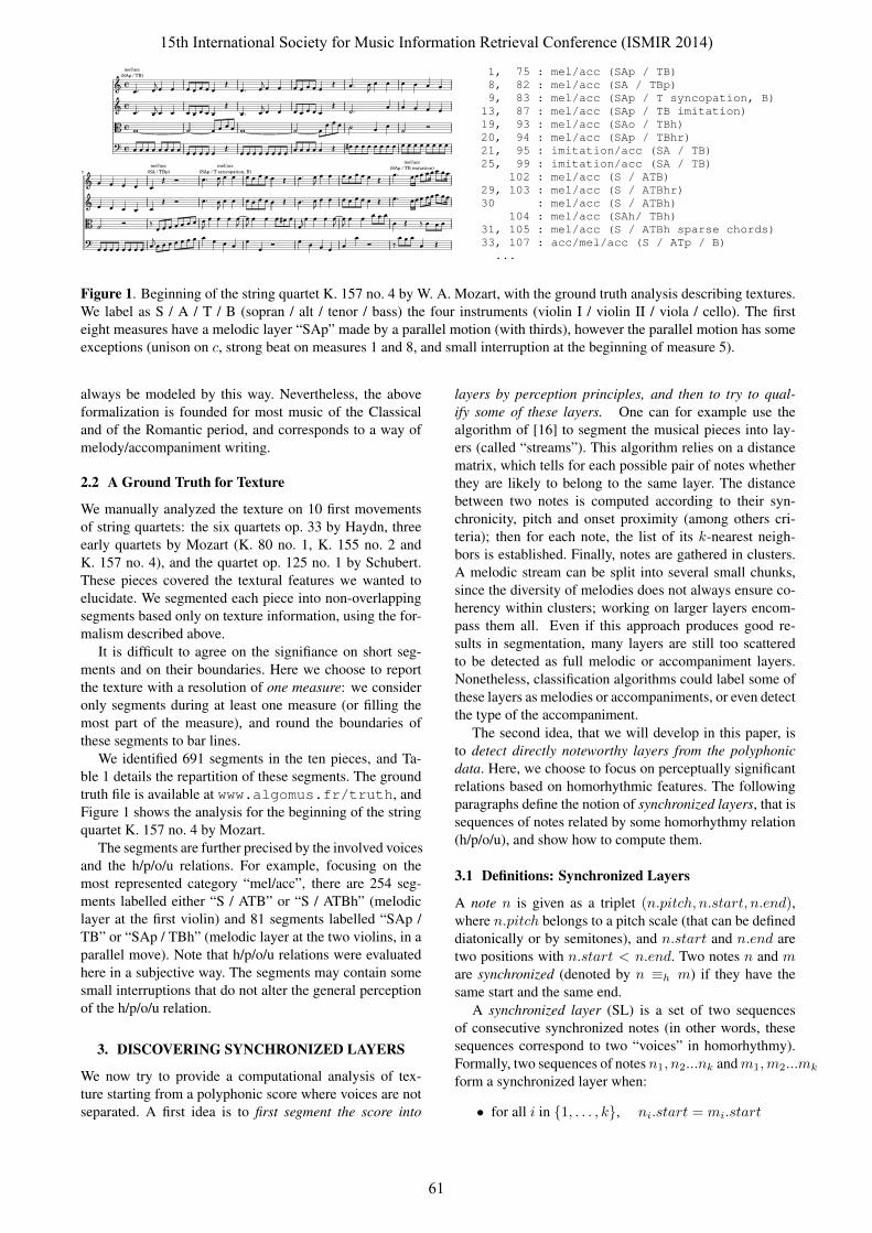
Figure 1. Beginning of the string quartet K. 157 no. 4 by W. A. Mozart, with the ground truth analysis describing textures.We label as S / A / T / B (sopran / alt / tenor / bass) the four instruments (violin I / violin II / viola / cello). The firsteight measures have a melodic layer “SAp” made by a parallel motion (with thirds), however the parallel motion has someexceptions (unison on c, strong beat on measures 1 and 8, and small interruption at the beginning of measure 5).

always be modeled by this way. Nevertheless, the aboveformalization is founded for most music of the Classicaland of the Romantic period, and corresponds to a way ofmelody/accompaniment writing.

2.2 A Ground Truth for Texture

We manually analyzed the texture on 10 first movementsof string quartets: the six quartets op. 33 by Haydn, threeearly quartets by Mozart (K. 80 no. 1, K. 155 no. 2 andK. 157 no. 4), and the quartet op. 125 no. 1 by Schubert.These pieces covered the textural features we wanted toelucidate. We segmented each piece into non-overlappingsegments based only on texture information, using the for-malism described above.

It is difficult to agree on the signifiance on short seg-ments and on their boundaries. Here we choose to reportthe texture with a resolution of one measure: we consideronly segments during at least one measure (or filling themost part of the measure), and round the boundaries ofthese segments to bar lines.

We identified 691 segments in the ten pieces, and Ta-ble 1 details the repartition of these segments. The groundtruth file is available at www.algomus.fr/truth, andFigure 1 shows the analysis for the beginning of the stringquartet K. 157 no. 4 by Mozart.

The segments are further precised by the involved voicesand the h/p/o/u relations. For example, focusing on themost represented category “mel/acc”, there are 254 seg-ments labelled either “S / ATB” or “S / ATBh” (melodiclayer at the first violin) and 81 segments labelled “SAp /TB” or “SAp / TBh” (melodic layer at the two violins, in aparallel move). Note that h/p/o/u relations were evaluatedhere in a subjective way. The segments may contain somesmall interruptions that do not alter the general perceptionof the h/p/o/u relation.

3. DISCOVERING SYNCHRONIZED LAYERS

We now try to provide a computational analysis of tex-ture starting from a polyphonic score where voices are notseparated. A first idea is to first segment the score into

layers by perception principles, and then to try to qual-ify some of these layers. One can for example use thealgorithm of [16] to segment the musical pieces into lay-ers (called “streams”). This algorithm relies on a distancematrix, which tells for each possible pair of notes whetherthey are likely to belong to the same layer. The distancebetween two notes is computed according to their syn-chronicity, pitch and onset proximity (among others cri-teria); then for each note, the list of its k-nearest neigh-bors is established. Finally, notes are gathered in clusters.A melodic stream can be split into several small chunks,since the diversity of melodies does not always ensure co-herency within clusters; working on larger layers encom-pass them all. Even if this approach produces good re-sults in segmentation, many layers are still too scatteredto be detected as full melodic or accompaniment layers.Nonetheless, classification algorithms could label some ofthese layers as melodies or accompaniments, or even detectthe type of the accompaniment.

The second idea, that we will develop in this paper, isto detect directly noteworthy layers from the polyphonicdata. Here, we choose to focus on perceptually significantrelations based on homorhythmic features. The followingparagraphs define the notion of synchronized layers, that issequences of notes related by some homorhythmy relation(h/p/o/u), and show how to compute them.

3.1 Definitions: Synchronized Layers

A note n is given as a triplet (n.pitch, n.start, n.end),where n.pitch belongs to a pitch scale (that can be defineddiatonically or by semitones), and n.start and n.end aretwo positions with n.start < n.end. Two notes n and mare synchronized (denoted by n ≡h m) if they have thesame start and the same end.

A synchronized layer (SL) is a set of two sequencesof consecutive synchronized notes (in other words, thesesequences correspond to two “voices” in homorhythmy).Formally, two sequences of notes n1, n2...nk andm1,m2...mk

form a synchronized layer when:

• for all i in {1, . . . , k}, ni.start = mi.start


61

tonality length mel/acc mel/mel acc/mel/acc acc/mel mel acc others h p o uHaydn op. 33 no. 1 B minor 91m 38 0 8 1 0 0 5 19 21 1 0Haydn op. 33 no. 2 E-flat major 95m 37 0 2 4 0 0 7 34 13 0 0Haydn op. 33 no. 3 C major 172m 68 0 0 0 3 13 6 29 50 1 0Haydn op. 33 no. 4 B-flat major 90m 25 0 1 0 0 0 6 16 6 0 0Haydn op. 33 no. 5 G major 305m 68 0 3 4 7 0 5 56 45 6 0Haydn op. 33 no. 6 D major 168m 58 0 1 3 15 0 29 43 42 0 2Mozart K. 80 no. 1 G major 67m 36 4 6 0 2 0 3 5 33 3 0Mozart K. 155 no. 2 D major 119m 51 0 0 0 1 0 0 21 32 4 1Mozart K. 157 no. 4 C major 126m 29 0 3 6 2 0 7 18 22 2 0

Schubert op. 125 no. 1 E-flat major 255m 102 0 0 0 20 2 0 54 8 46 21488m 512 4 24 18 50 15 68 295 272 63 5

Table 1. Number of segments in the ground truth analysis of the ten string quartets (first movements), and number ofh/p/o/u labels further describing these layers.

• for all i in {1, . . . , k}, ni.end = mi.end

• for all i in {1, . . . , k − 1}, ni.end = ni+1.start

This definition can be extended to any number of voices.As p/o/u relations have a strong musical signification, wewant to be able to enforce them. One can thus restrain therelation ≡h, considering the pitch information:

• we denote n ≡δ m if the interval between the twonotes n and m is δ. The nature of the interval δ de-pends on the pitch model: for example, the intervalcan be diatonic, such as in “third” (minor or major),or an approximation over the semitone information,such as in “3 or 4 semitones”. Some synchronizedlayers with ≡δ relations correspond to parallel mo-tions;

• we denote n ≡o m if notes n and m are separatedby any number of octaves;

• we denote n ≡u m where there is an exact equalityof pitches (unison).

Given a relation ≡∈{≡h,≡δ,≡o,≡u}, we say that asynchronized layer respects the relation ≡ if its notes arepairwise related according to this relation. The relation≡his an equivalence relation, but the restrained relations donot need to be equivalence relations: Some ≡δ relationsare not transitive.

For example, in Figure 1, there is between voices S andA (corresponding to violins I and II), in the first two mea-sures:

• a synchronized layer (≡h) on the two measures;

• and a synchronized layer (≡third) on the two mea-sures, except the first note.

Note that this does not correspond exactly to the “musical”ground truth (parallel move on at least the first four mea-sures) because of some rests and of the first synchronizednotes that are not in thirds.

A synchronized layer is maximal if it is not strictly in-cluded in another synchronized layer. Note that two maxi-mal synchronized layers can be overlapping, if they are notsynchronized. Note also that the number of synchronizedlayers may grow exponentially with the number of notes.

3.2 Detection of a Unique Synchronized Layer

A very noticeable textural effect is when all voices use thesame texture at the same time. For example, a sudden strik-ing unison raises the listener’s attention. We can first checkif all notes in a segment of the score belong to a unique syn-chronized layer (within some relation). For example, weconsider that all voices are in octave doubling or unison ifit lasts at least two quarters.

3.3 Detection of Maximal Synchronized Layers

In the general case, the texture has several layers, and thegoal is thus to extract layers using some of the notes. Re-member that we work on files where polyphony is not sepa-rated into voices: moreover, it is not always possible to ex-tract voices from a polyphonic score, for example on pianomusic. We want to extract maximal synchronized layers.However, as their number may grow exponentially withthe number of notes, we will compute only the start andend positions of maximal synchronized layers.

The algorithm is a kind of 1-dimension interval chain-ing [14]. The idea is as follows. Recursively, two voicesn1, . . . , nk andm1, . . . ,mk are synchronized if and only ifn1, . . . , nk−1 andm1, . . . ,mk−1 are synchronized, nk andmk are synchronized and finally nk−1.end = nk.start.Formally, the algorithm is described by the following:

Step 1. Compute a table with left-maximal SL. Build the tableleftmost start≡[j] containing, for each ending position j, the left-most starting position of a SL respecting ≡ ending in j. This canbe done by dynamic programming with the following recurrence:

leftmost start≡[j] =

min{leftmost start≡[i] | i ∈ S≡(j)}if S≡(j) is not empty

j if S≡(j) is empty

where S≡(j) is the set of all starting positions of synchronizednotes ending at j respecting the relation ≡:

S≡(j) =

{n.start

∣∣∣∣ there are two different notes n ≡ msuch that n.end = j

}

Step 2. Output only (left and right) maximal SL. Output (i, j)with i = leftmost start≡[j] for each j, such that j = max{jo | leftmost start≡[jo] = leftmost start≡[j]}


62

1 2 3 4 5 6 1 2 3 4 5 6 7 8 9 0 1 2 3 4 5 6 7 8 9 0 1 2 3 4 5 6 7 8 9 0 1 2 3 4 5 6 7 8 9 0 1 2 3 4 5 6 7 8 9 0 1 2 3 4 5 6 7 8 9 0 1 2 3 4 SA- SA- SA--- SA- SA- SA---- SA- SB- AB TB AT SB---- SA---- AB AT TB SA SA AB- SA AT SB- SB- ST-- 7 8 9 10 11 12 5 6 7 8 9 0 1 2 3 4 5 6 7 8 9 0 1 2 3 4 5 6 7 8 9 0 1 2 3 4 5 6 7 8 9 0 1 2 3 4 5 6 7 8 9 0 1 2 3 4 5 6 7 8 9 0 1 2 3 4 5 TB SA- SA- SA--- SA- SA- SA---- SA- SB- TB- TB AB AT AT SB ST-------- TB-- TB SA SA AB- SB- SB SB- SA ST AT-

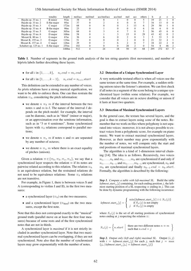
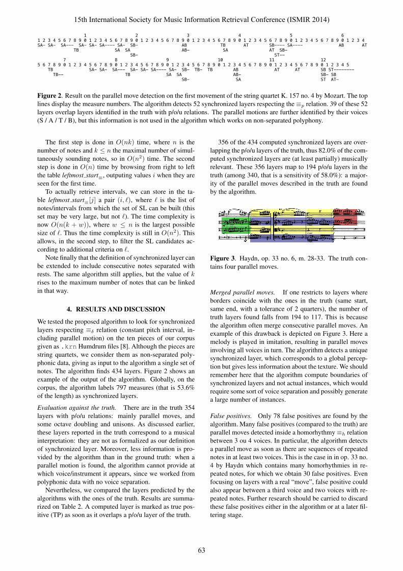
Figure 2. Result on the parallel move detection on the first movement of the string quartet K. 157 no. 4 by Mozart. The toplines display the measure numbers. The algorithm detects 52 synchronized layers respecting the≡p relation. 39 of these 52layers overlap layers identified in the truth with p/o/u relations. The parallel motions are further identified by their voices(S / A / T / B), but this information is not used in the algorithm which works on non-separated polyphony.

The first step is done in O(nk) time, where n is thenumber of notes and k ≤ n the maximal number of simul-taneously sounding notes, so in O(n2) time. The secondstep is done in O(n) time by browsing from right to leftthe table leftmost start≡, outputing values i when they areseen for the first time.

To actually retrieve intervals, we can store in the ta-ble leftmost start≡[j] a pair (i, `), where ` is the list ofnotes/intervals from which the set of SL can be built (thisset may be very large, but not `). The time complexity isnow O(n(k + w)), where w ≤ n is the largest possiblesize of `. Thus the time complexity is still in O(n2). Thisallows, in the second step, to filter the SL candidates ac-cording to additional criteria on `.

Note finally that the definition of synchronized layer canbe extended to include consecutive notes separated withrests. The same algorithm still applies, but the value of krises to the maximum number of notes that can be linkedin that way.

4. RESULTS AND DISCUSSION

We tested the proposed algorithm to look for synchronizedlayers respecting ≡δ relation (constant pitch interval, in-cluding parallel motion) on the ten pieces of our corpusgiven as .krn Humdrum files [8]. Although the pieces arestring quartets, we consider them as non-separated poly-phonic data, giving as input to the algorithm a single set ofnotes. The algorithm finds 434 layers. Figure 2 shows anexample of the output of the algorithm. Globally, on thecorpus, the algorithm labels 797 measures (that is 53.6%of the length) as synchronized layers.

Evaluation against the truth. There are in the truth 354layers with p/o/u relations: mainly parallel moves, andsome octave doubling and unisons. As discussed earlier,these layers reported in the truth correspond to a musicalinterpretation: they are not as formalized as our definitionof synchronized layer. Moreover, less information is pro-vided by the algorithm than in the ground truth: when aparallel motion is found, the algorithm cannot provide atwhich voice/instrument it appears, since we worked frompolyphonic data with no voice separation.

Nevertheless, we compared the layers predicted by thealgorithms with the ones of the truth. Results are summa-rized on Table 2. A computed layer is marked as true pos-itive (TP) as soon as it overlaps a p/o/u layer of the truth.

356 of the 434 computed synchronized layers are over-lapping the p/o/u layers of the truth, thus 82.0% of the com-puted synchronized layers are (at least partially) musicallyrelevant. These 356 layers map to 194 p/o/u layers in thetruth (among 340, that is a sensitivity of 58.0%): a major-ity of the parallel moves described in the truth are foundby the algorithm.

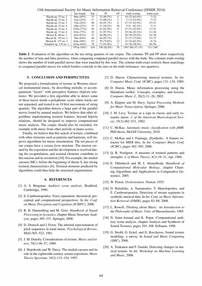
Figure 3. Haydn, op. 33 no. 6, m. 28-33. The truth con-tains four parallel moves.

Merged parallel moves. If one restricts to layers whereborders coincide with the ones in the truth (same start,same end, with a tolerance of 2 quarters), the number oftruth layers found falls from 194 to 117. This is becausethe algorithm often merge consecutive parallel moves. Anexample of this drawback is depicted on Figure 3. Here amelody is played in imitation, resulting in parallel movesinvolving all voices in turn. The algorithm detects a uniquesynchronized layer, which corresponds to a global percep-tion but gives less information about the texture. We shouldremember here that the algorithm compute boundaries ofsynchronized layers and not actual instances, which wouldrequire some sort of voice separation and possibly generatea large number of instances.

False positives. Only 78 false positives are found by thealgorithm. Many false positives (compared to the truth) areparallel moves detected inside a homorhythmy≡h relationbetween 3 ou 4 voices. In particular, the algorithm detectsa parallel move as soon as there are sequences of repeatednotes in at least two voices. This is the case in in op. 33 no.4 by Haydn which contains many homorhythmies in re-peated notes, for which we obtain 30 false positives. Evenfocusing on layers with a real “move”, false positive couldalso appear between a third voice and two voices with re-peated notes. Further research should be carried to discardthese false positives either in the algorithm or at a later fil-tering stage.


63

hits length hits TP FP truth-overlap truth-exactHaydn op. 33 no. 1 40m (44%) 37 32 (86.5%) 5 14 / 22 (63.6%) 7 / 22Haydn op. 33 no. 2 21m (22%) 17 15 (88.2%) 2 7 / 13 (53.9%) 7 / 13Haydn op. 33 no. 3 73m (42%) 48 44 (91.7%) 4 27 / 51 (52.9%) 15 / 51Haydn op. 33 no. 4 19m (21%) 47 17 (36.2%) 30 5 / 6 (83.3%) 3 / 6Haydn op. 33 no. 5 235m (77%) 58 47 (81.0%) 11 27 / 51 (52.9%) 11 / 51Haydn op. 33 no. 6 63m (37%) 24 21 (87.5%) 3 19 / 44 (43.2%) 11 / 44Mozart K. 80 no. 1 45m (67%) 27 26 (96.3%) 1 20 / 36 (55.6%) 14 / 36Mozart K. 155 no. 2 76m (64%) 46 44 (95.7%) 2 27 / 37 (73.0%) 15 / 37Mozart K. 157 no. 4 62m (49%) 52 39 (75.0%) 13 15 / 24 (62.5%) 8 / 24

Schubert op. 125 no. 1 163m (64%) 78 71 (91.0%) 7 33 / 56 (58.9%) 20 / 56797m (54%) 434 356 (82.0%) 78 194 / 340 (57.1%) 111 / 340

Table 2. Evaluation of the algorithm on the ten string quartets of our corpus. The columns TP and FP show respectivelythe number of true and false positives, when comparing computed parallel moves with the truth. The columns truth-overlapshows the number of truth parallel moves that were matched by this way. The column truth-exact restricts these matchingsto computed parallel moves for which borders coincide to the ones in the truth (tolerance: two quarters).

5. CONCLUSION AND PERSPECTIVES

We proposed a formalization of texture in Western classi-cal instrumental music, by describing melodic or accom-paniment “layers” with perceptive features (h/p/o/u rela-tions). We provided a first algorithm able to detect someof these layers inside a polyphonic score where tracks arenot separated, and tested it on 10 first movements of stringquartets. The algorithm detects a large part of the parallelmoves found by manual analysis. We believe that other al-gorithms implementing textural features, beyond h/p/o/urelations, should be designed to improve computationalmusic analysis. The corpus should also be extended, forexample with music from other periods or piano scores.

Finally, we believe that this search of texture, combinedwith other elements such as patterns and harmony, will im-prove algorithms for music structuration. The ten pieces ofour corpus have a sonata form structure. The tension cre-ated by the exposition and the development is resolved dur-ing the recapitulation, and textural elements contribute tothis tension and its resolution [10]. For example, the medialcaesura (MC), before the beginning of theme S, has strongtextural characteristics [6]. Textural elements predicted byalgorithms could thus help the structural segmentation.

6. REFERENCES

[1] A. S. Bregman. Auditory scene analysis. Bradford,Cambridge, 1990.

[2] E. Cambouropoulos. Voice separation: theoretical, per-ceptual and computational perspectives. In Int. Conf.on Music Perception and Cognition (ICMPC), 2006.

[3] R. B. Dannenberg and M. Goto. Handbook of SignalProcessing in Acoustics, chapter Music Structure Anal-ysis, pages 305–331. Springer, 2008.

[4] D. Deutsch and J. Feroe. The internal representation ofpitch sequences in tonal music. Psychological Review,88(6):503–522, 1981.

[5] J. M. Dunsby. Considerations of texture. Music and let-ters, 70(1):46–57, 1989.

[6] J. Hepokoski and W. Darcy. The medial caesura and itsrole in the eighteenth-century sonata exposition. MusicTheory Spectrum, 19(2):115–154, 1997.

[7] D. Huron. Characterizing musical textures. In Int.Computer Music Conf. (ICMC), pages 131–134, 1989.

[8] D. Huron. Music information processing using theHumdrum toolkit: Concepts, examples, and lessons.Computer Music J., 26(2):11–26, 2002.

[9] A. Klapuri and M. Davy. Signal Processing Methodsfor Music Transcription. Springer, 2006.

[10] J. M. Levy. Texture as a sign in classic and early ro-mantic music. J. of the American Musicological Soci-ety, 35(3):482–531, 1982.

[11] C. McKay. Automatic music classification with jMIR.PhD thesis, McGill University, 2010.

[12] C. McKay and I. Fujinaga. jSymbolic: A feature ex-tractor for MIDI files. In Int. Computer Music Conf.(ICMC), pages 302–305, 2006.

[13] Q. R. Nordgren. A measure of textural patterns andstrengths. J. of Music Theory, 4(1):19–31, Apr. 1960.

[14] E. Ohlebusch and M. I. Abouelhoda. Handbook ofComputational Molecular Biology, chapter Chain-ing Algorithms and Applications in Comparative Ge-nomics. 2005.

[15] W. Piston. Orchestration. Norton, 1955.

[16] D. Rafailidis, A. Nanopoulos, Y. Manolopoulos, andE. Cambouropoulos. Detection of stream segments insymbolic musical data. In Int. Conf. on Music Informa-tion Retrieval (ISMIR), pages 83–88, 2008.

[17] L. Rowell. Thinking about Music: An Introduction tothe Philosophy of Music. Univ. of Massachusetts, 1985.

[18] N. Saint-Arnaud and K. Popat. Computational audi-tory scene analysis. chapter Analysis and Synthesis ofSound Textures, pages 293–308. Erlbaum, 1998.

[19] G. Strobl, G. Eckel, and D. Rocchesso. Sound texturemodeling: a survey. In Sound and Music Computing(SMC), 2006.

[20] A. Tenkanen and F. Gualda. Detecting changes in mu-sical texture. In Int. Workshop on Machine Learningand Music, 2008.


64

towards modeling texture in symbolic data · towards modeling texture in symbolic data mathieu...

Documents