towards mechanical characterization of granular biofilms

Towards Mechanical Characterization of Granular Biofilms by Optical Coherence Elastography Measurements of

Circumferential Elastic Waves

Journal: Soft Matter

Manuscript ID SM-ART-04-2019-000739.R1

Article Type: Paper

Date Submitted by the Author: 08-Jun-2019

Complete List of Authors: Liou, Hong-Cin; Northwestern University, Mechanical EngineeringSabba, Fabrizio; Northwestern University, Civil and Environmental Engineering Packman, Aaron; Northwestern University, Civil and Environmental EngineeringRosenthal, Alex; Northwestern University, Civil and Environmental EngineeringWells, George; Northwestern University, Civil and Environmental EngineeringBalogun, Oluwaseyi; Northwestern University, Mechanical Engineering; Northwestern University, Civil and Environmental Engineering

Soft Matter

1

Towards Mechanical Characterization of Granular Biofilms by

Optical Coherence Elastography Measurements of


Hong-Cin Liou1, Fabrizio Sabba2, Aaron I. Packman2, Alex Rosenthal2, George Wells2,

Oluwaseyi Balogun1,2*

1Mechanical Engineering Department, Northwestern University, Evanston, IL 60208

2Civil and Environmental Engineering Department, Northwestern University, Evanston, IL

60208

*Corresponding author:

Oluwaseyi Balogun, Phone: +1 847-491-3054; e-mail: [email protected]

Page 1 of 37 Soft Matter

2

ABSTRACT

Microbial granular biofilms are spherical, multi-layered aggregates composed of communities of bacterial

cells encased in a complex matrix of hydrated extracellular polymeric substances (EPS). While granular

aggregates are increasingly used for applications in industrial and municipal wastewater treatment, their

underlying mechanical properties are poorly understood. The challenges of viscoelastic characterization for

these structures are due to their spherical geometry, spatially heterogeneous properties, and their delicate

nature. In this study, we report a model-based approach for nondestructive characterization of viscoelastic

properties (shear modulus and shear viscosity) of alginate spheres with different concentrations, which was

motivated by our measurements in granular biofilms. The characterization technique relies on experimental

measurements of circumferential elastic wave speeds as a function of frequency in the samples using the

Optical Coherence Elastography (OCE) technique. A theoretical model was developed to estimate the

viscoelastic properties of the samples from OCE data through inverse analysis. This work represents the

first attempt to explore elastic waves for mechanical characterization of granular biofilms. The combination

of the OCE technique and the theoretical model presented in this paper provides a framework that can

facilitate quantitative viscoelastic characterization of samples with curved geometries and the study of the

relationships between morphology and mechanical properties in granular biofilms.

Keywords: optical coherence elastography, nondestructive mechanical characterization, viscoelastic

properties, circumferential elastic waves, granular biofilms

Page 2 of 37Soft Matter

3

1. Introduction

Granular biofilms are microbial aggregates composed of multispecies bacterial cells and

extracellular polymeric substances (EPS) produced by microorganisms. The size of granular biofilms is

typically at the millimeter scale1-4. In recent years, granular biofilms have generated great interest for

wastewater treatment1, 2; compared to their predecessor—flocculent activated sludge—that is widely used

in wastewater treatment systems, granular biofilms provide several advantages including higher biomass

density, stronger cohesiveness, shorter settling time, higher energy efficiency, and less volume required,

which leads to a better operational efficiency of wastewater treatment1-4. However, despite these beneficial

attributes, the number of full-scale municipal or industrial systems utilizing granular biofilms is limited4, 5.

One reason for their limited use stems from the limited knowledge about the granulation mechanisms that

are crucial to controlling the granular biofilms’ growth in wastewater treatment systems in a predictable

and reproducible fashion2, 4, 6.

EPS plays an important role in forming the network structure and providing bonding to increase

the cohesiveness of microbial aggregates, which ultimately makes the topology of granular biofilms

different from flocculent sludge1-3, 5, 7-10. The material properties of biofilms are thought to be controlled in

part by EPS11. EPS contains polymers produced by bacteria such as proteins, polysaccharides, and nucleic

acids2. Over the last few decades, researchers have investigated the physical properties of EPS5, 12-16, and

these studies suggested that granular biofilms are analogous to hydrogels, particularly in regard to their EPS

composition, since they share similar viscoelastic properties. For example, the behavior of EPS is solid-like

under small strains as the storage (shear) modulus G’ is always larger than the loss modulus G”, while

under large strains, G” may exceed G’ so that the EPS is prone to be liquid-like5, 12-14. Rheometry tests also

showed that granular biofilms are shear-thinning fluids with yield pseudoplasticity3, 5, 11-14. It is worth

highlighting that for hydrogels, the gelation phenomenon results from the cross-linking of polymer chains,

and the cross-link density is related to the storage modulus G’5, 17. These discoveries suggest that the

viscoelastic behavior of EPS is critical to the granulation of granular biofilms and studying their viscoelastic


4

properties may further elucidate the key factors required to produce mechanically stable, predictable, and

controllable biological aggregates.

Rheometry is a common technique for viscoelastic characterization; however, in the context of

granular biofilms, it presents several limitations such as the inability to probe spatially heterogeneous

mechanical properties and the inability to conduct measurements with biofilms in their native aqueous

solutions. Optical Coherence Elastography (OCE) is a powerful alternative that overcomes these limitations

of rheometry18-20. OCE has been used for viscoelastic characterization of soft biological materials,

particularly in biomedical engineering to evaluate tissue mechanical properties21-26. OCE allows for 3D

nondestructive imaging of mechanical properties with (1) high spatial resolution at micron-scale, (2) high

displacement sensitivity at the nanoscale which minimizes the required magnitude of the external load,

preventing large disturbances in the sample, and (3) high sampling rate at 101~102 kHz that enables real-

time monitoring of the sample deformation. Moreover, the OCE image is co-registered with the Optical

Coherence Tomography (OCT) image that shows sample’s important internal structural features, such as

pores in the matrix, which provides a useful tool to study the relationship between the sample morphology

and mechanical properties27.

Recently, a dynamic OCE approach that relies on measurements of elastic wave propagation was

shown to be suitable for characterizing the shear modulus and complex shear viscosity of a mixed-culture

biofilm with plate-like geometry28. While the plate-like biofilm was explored to demonstrate the feasibility

of mechanical characterization in environmental biofilms using OCE, broadening application of this

technique to granular biofilms is challenging due to their curved geometries and depth-dependent properties

that significantly complicate the elastic wave propagation.

In this paper, we report the OCE measurements of elastic wave propagation in a granular biofilm

and a theoretical model that is capable of predicting the dispersion (frequency-dependent wave speed) of

circumferential elastic waves in a cylindrical viscoelastic solid. The model can approximate the propagation

of elastic waves along a circular contour of fixed radius in a spherical sample, and is used for inverse

analysis to estimate the viscoelastic properties from OCE measurements of elastic wave propagation. The


5

inverse analysis approach was validated on alginate spheres with two different concentrations, from which

their shear moduli and complex shear viscosities were obtained. We chose alginate as a model system for

the OCE measurements because it is commonly present in granular biofilm EPS7, 11, 15. The combination of

the modeling and experimentation approaches reported in this paper presents a promising framework

towards nondestructive characterization of viscoelastic properties in practical environmental biofilms with

curved geometries.

2. Materials and methods

2.1 Sample preparation

Granular biofilms obtained from a full-scale AquaNereda Aerobic Granular Sludge (AGS) Reactor (Aqua-

Aerobic Systems, Inc., Rockford, IL, USA) and soft alginate gel samples were characterized with the OCE

technique. Spherical alginate (Acros Organics, NJ, USA) samples with 0.8% and 1.2% weight-to-volume

(w/v) concentrations were prepared. Mixtures of the two different concentrations were obtained by mixing

0.8 and 1.2 grams of alginate powder, respectively, with a 100 mL solution made from 70 mL of

nanopurified water and 30 mL of 5.0% w/v skim milk (Becton, Dickinson and Company 232100, MD,

USA). The skim milk was used to increase the optical scattering from the transparent alginate spheres and

enhance the OCT image contrast. The alginate solution was stirred in a capped 250 mL Pyrex bottle using

a magnetic stir bar with a stir plate (operated at ~400 rpm and heated at 100oC) for one hour. Subsequently,

the mixture was removed from the stir plate and held at ambient temperature for ~30 minutes to remove

entrained air bubbles. Alginate spheres were formed by dripping the mixture into a cross-linking agent

made from 25% w/v potassium nitrate and 2% w/v calcium chloride (adapted from Chang and Tseng29).

The mixture was ejected slowly from a 5 mL pipet tip held horizontally and 10 cm above the surface of the

cross-linking agent. Slow ejection speeds were used to ensure that the weight of the droplet was balanced

by surface tension, and the droplet hung near the edge of the pipet tip. During the ejection, the size of the

droplet increased until a critical volume was reached, and, as the weight exceeded the surface tension, the

droplet detached from the pipet tip and fell into the cross-linking agent. The droplet’s spherical shape was


6

formed by surface tension during its free-fall into the cross-linking agent29. The spherical droplets solidified

in the agent after curing for approximately 30 minutes. OCE experiments were conducted on the cured

alginate spheres after 72 hours to ensure that the agent fully diffused through each of them. The process for

preparing the alginate spheres is highly repeatable, and the diameter of the spheres falls within the range of

3-5 mm.

2.2 Experimental setup

A schematic of the experimental configuration is shown in Fig. 1. The setup was used to generate and

monitor elastic wave propagation in the samples. The waves were excited by a paddle actuator in light

contact with the sample surface. The actuator was composed of a razor blade, an 18-gauge syringe needle,

and a piezoelectric transducer (Thorlabs PZS001, NJ, USA) driven by a radio frequency function generator

(Agilent 33120A, CA, USA). The function generator applied a sinusoidal voltage to the transducer to move

the needle-blade assembly harmonically along its length, leading to small periodic indentation on the

sample surface that generates the harmonic compressional, shear, and circumferential elastic waves. The

compressional and shear waves propagate through the interior regions of the sample, and they could be

reflected back into the sample or transmitted into the surrounding fluid at the sample boundaries. On the

other hand, circumferential waves travel along the curved boundary of the sample, exhibiting frequency-

dependent wave speeds and penetration depths. The sample was submerged in water during the experiment

to preserve the moisture content and to prevent changes to the material properties (not shown in Fig. 1).

The local displacement induced by the propagating elastic waves was monitored by a phase-

sensitive, spectral-domain OCT microscope (Thorlabs GAN210C1). The OCT’s imaging mechanism and

the method used to synchronize the wave frequency and the scanning rate of the OCT were detailed in our

previously published work28. The OCT microscope provides two types of image output: (1) the intensity

distribution corresponding to the optical scattering from a partially transparent sample due to refractive

index variation in the sample (the refractive index variation results from sample’s morphology) and (2) the


7

distribution of the optical phase difference that is related to the local particle displacement in the sample. Δ𝜙

These two types of images will be referred as OCT and OCE images, respectively, in this paper.

3. OCE measurements in a granular biofilm

Figure 2 shows representative OCT and OCE images obtained in a granular biofilm. The sample was

submerged in its native aqueous solution from the AGS reactor. The OCT image (Fig. 2a) shows the curved

geometry of the granular biofilm. The intensity of the OCT signal decreases with depth from the surface of

the biofilm due to attenuation of the probe light, showing that the optical penetration depth is less than 1

mm. Furthermore, the sharp intensity gradient observed near the inner boundary of the biofilm separates

the biofilm into an outer bright layer and an inner dark core. The lower signal intensity of the latter is

possibly due to the contrasts of the morphology or density in the biofilm2, 3. The thickness of the outer layer

remains relatively constant (~0.75 mm) within a lateral extent of ~2 mm and reduces monotonically with

an abrupt curvature change near the right edge of the OCT image. The OCE image (Fig. 2b) shows the

distribution of that corresponds to the deformation induced by a 2.1 kHz elastic wave confined along Δ𝜙

the biofilm boundary. The local signal is proportional to the vertical particle displacement. Note that Δ𝜙

Δϕ is an interferometric parameter that alternates between –π to π radians, but to enhance visibility of the

fringes, the color contour in the OCE image was modified to saturate at the limits –π/2 and π/2 radians. The

fringes of the signal within the constant-thickness region yields a wavelength estimate of 1.8 mm Δ𝜙

(corresponding to the wave speed of 3.78 m/s). It is worth remarking that (1) the apparent wavelength close

to the right edge of the biofilm is longer than 1.8 mm due to the change in elastic properties or curvature

relative to the left portion of the biofilm, and (2) the elastic wave also interacts with the surrounding fluid,

propagating as an interface wave whose amplitude decays with vertical distance into the fluid and the

biofilm. Note that in an infinite homogenous elastic solid, the elastic wave speeds of the bulk compressional

and shear waves can be directly related to the elastic properties since the wave speeds are frequency- and

geometry-independent. However, in the granular biofilm, the elastic wave speed is highly sensitive to the

sample heterogeneity, local curvature variation, and the properties of the surrounding fluid. Therefore, to


8

determine the viscoelastic properties from the OCE data obtained in the granular biofilm, an appropriate

inverse modeling approach is needed. The details of the theoretical model developed for this purpose is

discussed in the next section.

4. Theoretical model

In this section, a theoretical model for calculating the frequency-dependent phase velocity of

circumferential elastic waves in a viscoelastic solid with curved geometry is presented. This model was

used to quantify the shear modulus and complex shear viscosity of the alginate gel samples though inverse

analysis from experimental measurements. To reduce modeling complexity, a two-layer cylindrical

geometry illustrated in Fig. 3 was adopted. The inner and outer radii of the cylinder are labeled as a and b,

respectively. The cylinder is surrounded by an inviscid water half-space (r > b) that does not support shear

stresses, and all material properties in this structure are homogeneous and isotropic. It has been shown that

the waveform supported on the surface of a homogeneous and isotropic sphere is toroidal30, 31. The

propagation of a toroidal wave can be monitored by probing only on the meridian circle that is normal to

the wavefront. As such, the toroidal wave propagation can be approximated by the circumferential wave

that travels on the surface of a cylinder with the same curvature of the meridian circle. Therefore, the

cylindrical configuration of this model structure is valid and provides a simple approach for modeling the

key features of the wave observed in Fig. 2b that is of particular interest to this work: (1) a circumferential

wave that travels along a circular contour, and (2) an interface wave (or Sholte wave32) that propagates at

the interface between the solid and the water.

The elastodynamic wave equation formulated in cylindrical coordinates for harmonic wave

propagation in a homogeneous, isotropic, and viscoelastic solid is expressed as33

(1)(𝜆 ∗ + 𝜇 ∗ )∇(∇ ∙ 𝑢) + 𝜇 ∗ ∇2𝑢 + 𝜌𝜔2𝑢 = 0


9

where the displacement vector comprises the components , , and along r-, 𝑢 = 𝑢𝑟𝑒𝑟 + 𝑢𝜃𝑒𝜃 + 𝑢𝑧𝑒𝑧 𝑢𝑟 𝑢𝜃 𝑢𝑧

θ-, and z-directions with unit vectors , , and ; is the density of the material; is the angular 𝑒𝑟 𝑒𝜃 𝑒𝑧 𝜌 𝜔

frequency; is the differential operator defined by∇

. (2)∇ = 𝑒𝑟∂

∂𝑟 + 𝑒𝜃1𝑟

∂∂𝜃 + 𝑒𝑧

∂∂𝑧

In eqn (1), and are the complex frequency-dependent relaxation functions of the Lamé 𝜆 ∗ 𝜇 ∗

material properties. Following the Kelvin-Voigt viscoelastic model, the relaxation functions are32

(3)λ ∗ (𝜔) = 𝜆 + 𝑖𝜂𝜆𝜔

(4)𝜇 ∗ (𝜔) = 𝜇 + 𝑖𝜂𝜇𝜔

where and are the Lamé first parameter and shear modulus, respectively, and and are the 𝜆 𝜇 𝜂𝜆 𝜂𝜇

corresponding complex viscosities, respectively. The shear modulus and the shear viscosity are of 𝜇 𝜂𝜇

particular interest in this study.

It can be shown that the solution to eqn (1) is a linear superposition of the contributions from 𝑢

compressional (longitudinal) and shear waves, which can be expressed in terms of a scalar potential and 𝜙

a vector potential by the vector relationship33:𝜓 = (𝜓𝑟,𝜓𝜃,𝜓𝑧)

(5)𝑢 = ∇𝜙 + ∇ × 𝜓

To consider only the plane circumferential interface waves, plane strain conditions are imposed on

the displacements and stresses such that (1) the displacement component in the z-direction vanishes ( ), 𝑢𝑧 = 0

and (2) gradients along the z-direction are zero ( ). From the first condition, the first two ∂/∂𝑧 = 0

components of must equal to zero ( ), yielding . From the second condition, the 𝜓 𝜓𝑟 = 𝜓𝜃 = 0 𝜓 = (0,0,𝜓)

third term of the differential operator in eqn (2) vanishes.

Substituting eqn (5) into eqn (1) leads to the Helmholtz equations for the scalar and vector potentials:

(6)( ∂2

∂𝑟2 +1𝑟

∂∂𝑟 +

1𝑟2

∂2

∂𝜃2)𝜙 +𝜔2

𝛼2𝐿𝜙 = 0

(7)( ∂2

∂𝑟2 +1𝑟

∂∂𝑟 +

1𝑟2

∂2

∂𝜃2)𝜓 +𝜔2

𝛼2𝑆𝜓 = 0


10

where and are complex compressional and shear wave speeds that are related to the material properties 𝛼𝐿 𝛼𝑆

by the relationships:

(8)𝛼2𝐿 =

𝜆 ∗ + 2𝜇 ∗ 𝜌

(9)𝛼2𝑆 =

𝜇 ∗ 𝜌

The real parts of and are the bulk compressional and shear wave speeds, respectively, and the 𝛼𝐿 𝛼𝑆

imaginary parts determine the attenuation (amplitude decay with propagation distance) of the bulk waves.

Following related work in the literature34, 35, the scalar and vector potential functions corresponding

to circumferential interface waves in the solid cylinder are defined as

(10)𝜙 = Φ(𝑟)𝑒𝑖(𝑘𝑏𝜃 ― 𝜔𝑡)

(11)𝜓 = Ψ(𝑟)𝑒𝑖(𝑘𝑏𝜃 ― 𝜔𝑡)

where and represent the complex amplitudes along the radial (r) direction; k is the complex Φ(𝑟) Ψ(𝑟)

wavenumber whose real part is related to the wavelength by and imaginary part Re{𝑘} = 𝑘𝑅 𝜆 𝑘𝑅 = 2𝜋/𝜆

represents the wave attenuation.

From eqn (6), (7), (10) and (11), we obtain the following differential equations that and Φ(𝑟) Ψ(𝑟)

must satisfy:

(12)𝑑2Φ𝑑𝑟2 +

1𝑟

𝑑Φ𝑑𝑟 + (𝑘2

𝐿 ―𝑘2𝑏2

𝑟2 )Φ = 0

(13)𝑑2Ψ𝑑𝑟2 +

1𝑟

𝑑Ψ𝑑𝑟 + (𝑘2

𝑆 ―𝑘2𝑏2

𝑟2 )Ψ = 0

where and are complex wavenumbers for the bulk compressional and shear waves.𝑘𝐿 = 𝜔/𝛼𝐿 𝑘𝑆 = 𝜔/𝛼𝑆

Eqn (12) and (13) are Bessel differential equations whose general solutions are linear

superpositions of Bessel functions as expressed below:

(14)Φ(𝑟) = 𝐴1𝐽𝜈(𝑘𝐿𝑟) + 𝐴2𝑌𝜈(𝑘𝐿𝑟)

(15)Ψ(𝑟) = 𝐴3𝐽𝜈(𝑘𝑆𝑟) + 𝐴4𝑌𝜈(𝑘𝑆𝑟)

where A1, A2, A3, and A4 are unknown coefficients, and are Bessel functions of the first and 𝐽𝜈(𝑥) 𝑌𝜈(𝑥)

second kind, and is the order of the Bessel functions.𝜈 = 𝑘𝑏


11

In cylindrical coordinates, the components of the particle displacement and the stress tensor have

the relationships with the scalar and vector potentials as below:

(16)𝑢𝑟 =∂𝜙∂𝑟 +

1𝑟

∂𝜓∂𝜃

(17)𝑢𝜃 =1𝑟

∂𝜙∂𝜃 ―

∂𝜓∂𝑟

(18)𝜎𝑟𝑟 = (𝜆 ∗ + 2𝜇 ∗ )∂2𝜙∂𝑟2 + 𝜆 ∗ (1

𝑟∂𝜙∂𝑟 +

1𝑟2

∂2𝜙∂𝜃2) +2𝜇 ∗ (1

𝑟∂2𝜓

∂𝑟∂𝜃 ―1𝑟2

∂𝜓∂𝜃)

(19)𝜎𝑟𝜃 = 𝜇 ∗ (2𝑟

∂2𝜙∂𝑟∂𝜃 ―

2𝑟2

∂𝜙∂𝜃 ―

∂2𝜓∂𝑟2 +

1𝑟

∂𝜓∂𝑟 +

1𝑟2

∂2𝜓∂𝜃2)

By substituting eqn (10) and (11) into eqn (16) – (19), using the expressions for and in Φ(𝑟) Ψ(𝑟)

eqn (14) and (15), the components of the particle displacement and the stress tensor can be expressed in

terms of the unknown coefficients and combined as the following matrix set:

(20)[ 𝑢𝑟𝑢𝜃𝜎𝑟𝑟𝜎𝑟𝜃

] = [𝐷11 𝐷12 𝐷13 𝐷14𝐷21 𝐷22 𝐷23 𝐷24𝐷31 𝐷32 𝐷33 𝐷34𝐷41 𝐷42 𝐷43 𝐷44

][𝐴1𝐴2𝐴3𝐴4

]𝑒𝑖(𝑘𝑏𝜃 ― 𝜔𝑡)

The expressions of the matrix elements Dmn (m,n = 1,2,3,4) in eqn (20) are provided in the Appendix.

The displacement and pressure in the surrounding water half-space are formulated in terms of a

scalar potential function . The displacement is given by the gradient of :𝜙𝑤 𝜙𝑤

(21)𝑢𝑤 = ∇𝜙𝑤

Eqn (21) does not include the vector potential because the water half-space is assumed to be inviscid

and does not support shear waves.

We specifically focused on the solution of the interface waves that are simultaneously coupled in

the solid and the water half-space. We formulated this by matching the phase of the scalar potential in the

water to that in the solid, such as

(22)𝜙𝑤 = Φ𝑤(𝑟)𝑒𝑖(𝑘𝑏𝜃 ― 𝜔𝑡)

where the complex amplitude must satisfy the Bessel differential equationΦ𝑤(𝑟)

(23)𝑑2Φ𝑤

𝑑𝑟2 +1𝑟

𝑑Φ𝑤

𝑑𝑟 + (𝑘2𝑤 ―

𝑘2𝑏2

𝑟2 )Φ𝑤 = 0


12

that is obtained by substituting eqn (22) into eqn (6). In eqn (23), is the wavenumber of the 𝑘𝑤 = 𝜔/𝛼𝑤𝐿

compressional wave as 1481 m/s is the wave speed in water. Because the water half-space is assumed 𝛼𝑤𝐿 =

to be inviscid, is a real number without the imaginary part. Moreover, the water half-space has no 𝛼𝑤𝐿

excitation source, as such, only the partial waves traveling outward in the radial direction exist in the water,

and the solution of eqn (23) is represented by the Hankel function of the first kind, given by

(24)Φ𝑤(𝑟) = 𝐴5𝐻(1)𝜈 (𝑘𝑤𝑟)

The unknown coefficient A5 is determined by the boundary conditions at the solid-water interface.

From eqn (16), (18), and (21) − (24), the displacement and the pressure (equivalent to the normal

stresses in the solid) along the radial direction in the water half-space are derived as functions of the

unknown coefficient A5:

(25)𝑢𝑤𝑟 = (𝑘𝑤𝐻(1)

𝜈 ′)𝐴5𝑒𝑖(𝑘𝑏𝜃 ― 𝜔𝑡)

(26)𝑝 = (𝜆𝑤𝑘2𝑤𝐻(1)

𝜈 ′′ + 𝜆𝑤1𝑟𝑘𝑤𝐻(1)

𝜈 ′ ― 𝜆𝑤𝜈2

𝑟2𝐻(1)𝜈 )𝐴5𝑒𝑖(𝑘𝑏𝜃 ― 𝜔𝑡) = 𝑃(𝑟)𝐴5𝑒𝑖(𝑘𝑏𝜃 ― 𝜔𝑡)

where

(27)𝐻(1)𝜈 = 𝐻(1)

𝜈 (𝑘𝑤𝑟), 𝐻(1)𝜈

′ =𝑑

𝑑(𝑘𝑤𝑟)(𝐻(1)𝜈 (𝑘𝑤𝑟)), 𝐻(1)

𝜈′′ =

𝑑2

𝑑(𝑘𝑤𝑟)2(𝐻(1)𝜈 (𝑘𝑤𝑟))

In eqn (26), is the Lamé first parameter for the water half-space that is related to the 𝜆𝑤

compressional wave speed and the water density by .𝛼𝑤𝐿 𝜌𝑤 𝜆𝑤 = 𝜌𝑤(𝛼𝑤

𝐿 )2

To determine the five unknown coefficients associated with the potential functions in the solid and

water, five boundary conditions are required. Here, we prescribe the inner boundary (r = a) to be rigid, so

the boundary conditions are (1) continuity of the displacement along radial direction at the water-sphere

interface, , (2) continuity of the normal traction in the solid and pressure in the water at 𝑢𝑟|𝑟 = 𝑏 = 𝑢𝑤𝑟 |𝑟 = 𝑏

the water-solid interface, , (3) zero shear traction at the water-solid interface, , 𝜎𝑟𝑟|𝑟 = 𝑏 = 𝑝|𝑟 = 𝑏 𝜎𝑟𝜃|𝑟 = 𝑏 = 0

(4) zero radial displacement at the inner boundary, , and (5) zero circumferential displacement 𝑢𝑟|𝑟 = 𝑎 = 0

at the inner boundary, . Applying these boundary conditions leads to five equations for the 𝑢𝜃|𝑟 = 𝑎 = 0

coefficients as shown in the matrix form below:


13

[𝐷11|𝑟 = 𝑏 𝐷12|𝑟 = 𝑏 𝐷13|𝑟 = 𝑏 𝐷14|𝑟 = 𝑏 ― 𝑘𝑤𝐻(1)𝜈 ′|𝑟 = 𝑏

𝐷31|𝑟 = 𝑏 𝐷32|𝑟 = 𝑏 𝐷33|𝑟 = 𝑏 𝐷34|𝑟 = 𝑏 ― 𝑃(𝑟)|𝑟 = 𝑏𝐷41|𝑟 = 𝑏 𝐷42|𝑟 = 𝑏 𝐷43|𝑟 = 𝑏 𝐷44|𝑟 = 𝑏 0𝐷11|𝑟 = 𝑎 𝐷12|𝑟 = 𝑎 𝐷13|𝑟 = 𝑎 𝐷14|𝑟 = 𝑎 0𝐷21|𝑟 = 𝑎 𝐷22|𝑟 = 𝑎 𝐷23|𝑟 = 𝑎 𝐷24|𝑟 = 𝑎 0

][𝐴1𝐴2𝐴3𝐴4𝐴5

] = 𝟎

or

(28)𝐒𝐀 = 𝟎

To obtain non-trivial solutions for unknown coefficients in matrix A of eqn (28), the determinant

of the matrix S must equal to zero36:

(29)det (𝐒) = 0

which is the characteristic equation of this model. Solving the characteristic equation yields infinite solution

pairs of angular frequency and complex wavenumber (𝜔,k) that represent the dispersion relation of the

plane circumferential interface wave in the water-loaded cylindrical solid. The phase velocity (c) of the

interface wave is obtained from the relation between the angular frequency ω and the real part of the

complex wavenumber , defined by . Since the matrix S is complex, eqn (29) is solved Re{𝑘} = 𝑘𝑅 𝑐 = 𝜔/𝑘𝑅

by searching the combinations of (𝜔,k) where the determinant of S has zero magnitude, |det(S)| = 0. Note

that it may be difficult to achieve absolute zero in numerical calculation; therefore, in practice, the solutions

are determined instead by locating local minima in the (𝜔,k) space. (see Section S1 of the Supplementary

Information for further details).

5. Results and discussion

5.1 Numerical simulation

The theoretical model presented in the previous section was implemented numerically in a commercial

software MATLAB (Release R2016b, MathWorks) to calculate the dispersion curves for the

circumferential elastic waves. The model was validated against a thin, pure-elastic curved plate with a very

small thickness to inner radius ratio (b − a)/a = 0.05, which approximates the curved plate to a flat plate.

The plate has the same parameters and boundary conditions as those reported by Liu and Qu (1998)34: a =


14

20 mm, b = a/0.95, αL = 5660 m/s, αS = 3200 m/s, and traction-free boundary conditions at the inner and

outer boundaries (r = a and b). The characteristic equation for this case is discussed in Section S2 of

Supplementary Information. The dispersion curves for the thin curved plate were calculated by our

MATLAB program, and the results are presented in Fig. 4 by plotting the normalized angular frequency 𝜔

against the normalized wavenumber , which is the same as the Fig. 2(c) in = 𝜔(𝑏 ― 𝑎)/𝛼𝑆 𝑘 = 𝑘(𝑏 ― 𝑎)

Liu and Qu (1998).

From Fig. 4, we observe that the dispersion curves for the thin curved plate resemble the

antisymmetric and symmetric guided wave modes in a thin flat plate—(1) the phase velocities of the two

lowest modes are strongly frequency-dependent at low frequencies, but become non-dispersive at high

frequencies, approaching the Rayleigh wave velocity; (2) the higher order modes originate at cut-off

frequencies defined by or (n = 1,2,3,…) for longitudinal or shear thickness 𝜔𝑐 = (𝛼𝐿/𝛼𝑆)𝑛𝜋 𝜔𝑐 = 𝑛𝜋

resonance modes, respectively. These resemblances, which are expected due to the flatness of the thin

curved plate, provide the validation for the circumferential elastic wave model. In addition, the dispersion

curves shown in Fig. 4 are identical to those calculated by Liu and Qu (1998), which verifies the correctness

of our MATLAB program. Note that the axis parameters for Fig. 4 were chosen to be the same as those

used by Liu and Qu34 for easy and direct comparison. For the other dispersion curves presented in this

paper, the phase velocity was plotted as a function of frequency. The dispersion curve of phase velocity is

directly relevant to the OCE measurements and will be used for inverse analysis to quantify the viscoelastic

properties.

Next, the dispersion curve for the lowest order mode is examined to understand the penetration

depth of the circumferential interface wave and how its phase velocity is affected by the viscoelastic

properties and the outer boundary curvature of the water-loaded model cylinder. The model material was

assumed to be homogeneous, isotropic biofilm with the density ρ = 1000 kg/m3, longitudinal wave speed

αL = 1481 m/s, and shear wave speed αS = 2 m/s. ρ and αL were chosen to be the same as water due to the


15

high ratio of water content (over 90%) in biofilms28. The boundary condition of the inner boundary (r = a)

was assumed to be rigid.

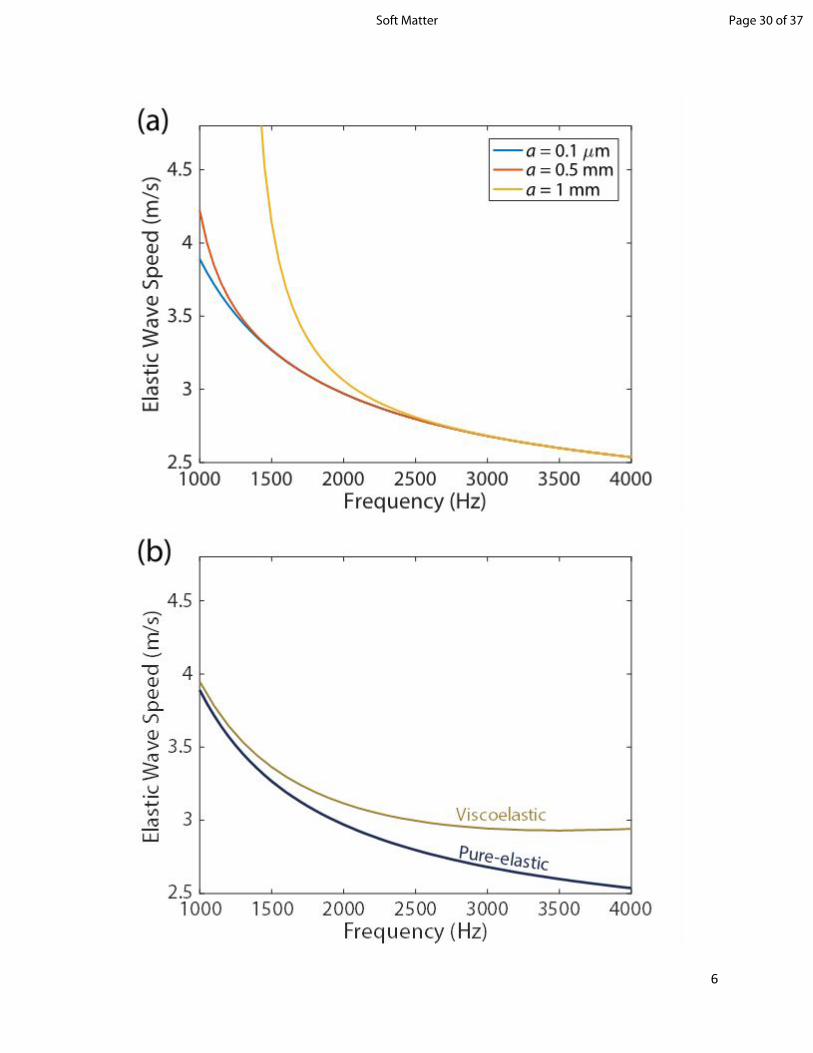
The penetration depth of the circumferential elastic wave is investigated by fixing the outer radius

b = 2 mm and changing the inner radius a of the cylinder. Figure 5a shows a series of dispersion curves for

three different inner radii a = 0.1 μm, 0.5 mm and 1 mm. The dispersion curves are plotted with the phase

velocity c and frequency f on the ordinate and abscissa axes, respectively, for convenience. All dispersion

curves originate from higher phase velocities at low frequency region and decrease monotonically with

frequency. The difference at low frequencies results from the cut-off frequencies of the modes for these

cases since the cut-off frequency increases with reduced thickness. The overall decreasing trends of the

dispersion curves imply that the penetration depths, which have positive correlation with the wavelengths

(determined by = c/f), also decrease with frequency for these three cases. Take the case a = 1 mm for

example, below 2700 Hz, the dispersion curve has higher phase velocity than other two cases since the

penetration depth is still larger or comparable to the thickness between the two boundaries (b − a = 1 mm)

so that the wave propagates as a guided wave that interacts with both boundaries of the cylinder. Above

2700 Hz, the penetration depth becomes smaller than all three thicknesses considered so that three

dispersion curves collapse on top of each other, indicating the wave propagates as an interface wave whose

energy is confined near the solid-water interface. At the transition frequency 2700 Hz, we may conclude

that the penetration depth of the interface wave is 1 mm, while the wavelength, calculated from the phase

velocity 2.75 m/s, is 1.02 mm, which confirms the common rule-of-thumb that the penetration depth of the

interface wave is approximately equal to one wavelength. This attribute of the interface wave may be

suitable for depth profiling of the viscoelastic properties in a radially gradient sample through

measurements of the frequency-dependent wave speeds.

The calculated dispersion curves for water-loaded pure-elastic and viscoelastic cylinders are

compared in Fig. 5b. For these calculations, the complex viscosity was changed from ημ = 0 for the pure-

elastic case to ημ = 0.1 Pa-s for the viscoelastic case. The inner and outer radii of the cylinder are a = 0.1

μm and b = 2 mm. For the pure-elastic cylinder, the phase velocity of the interface wave decreases


16

monotonically with frequency. On the other hand, the viscoelastic cylinder has similar decreasing phase

velocity at low frequencies but shows a flattened trend from 2500 Hz and a slight increase beyond 3500

Hz. This is because the complex shear modulus of the viscoelastic cylinder increases linearly with

frequency by the factor of the shear viscosity as defined in eqn (4). The increase in the phase velocity of

the interface wave at high frequencies is directly related to the viscoelastic properties of the material and

will be explored in this paper to characterize the complex shear modulus of the curved alginate gel samples.

Finally, the influence of the radius of curvature on the phase velocity of the interface wave in the

water-loaded viscoelastic cylinder is presented in Fig. 5c. Three different outer radii (b = 1.5 mm, 2 mm,

2.5 mm) were used in the calculations, while the inner radius was fixed to a = 0.1 μm. The shear viscosity

is the same as the viscoelastic case in Fig. 5b (ημ = 0.1 Pa-s). The dispersion curves in Fig. 5c show a clear

dependence of the phase velocity on the radius of curvature of the solid-water interface—the phase velocity

decreases with the radius of curvature. In addition, all dispersion curves show the flattened-to-increase

trends at high frequencies, which results from the escalating complex shear modulus with frequency by the

factor of shear viscosity as observed in Fig. 5b. The results suggest that the curvature of the interface plays

an important role in the frequency-dependent phase velocity of the interface wave. We will accommodate

the curvature effect in the analysis works in following sections.

5.2 Application of OCE and model-based inverse analysis to alginate gel spheres

Figure 6 shows representative OCT and OCE images for a 0.8% alginate sphere with a diameter of 4 mm

submerged in water. During the experiments, the water height was kept at least 2 mm higher than the top

of the sphere, so that the effect of the water surface on the circumferential interface waves was negligible.

The OCT image shows very limited intensity variation within the sample, indicating structural homogeneity

and the integrity (no voids or cracks) of the sample. The local intensity in the OCT image decreases with

depth below the sample surface due to attenuation of the OCT light source. The penetration depth of the

OCT light beam depends on the wavelength of light source and the optical properties of the sample. The

OCE image shows periodic oscillation of the optical phase difference Δϕ associated with the periodic


17

displacement profile of the elastic wave excited by the actuator at 1600 Hz. The displacement profile

follows the curvature of the sample surface, as expected for a circumferential interface wave. The amplitude

of the fringes decreases with the circumferential distance from the source due to damping in the viscoelastic

solid.

To determine the phase velocity of the circumferential wave, which equals to the product of the

excitation frequency and the wavelength, the wavelength was obtained from the fringes in the OCE image

by following four steps: (1) the contour of the sample surface in the OCT image was identified; (2) a circular

arc was fitted to the contour to determine the approximate radius of curvature and the propagation path

(white dotted line in Fig. 6b); (3) the spatial OCE data along the propagation path was processed by fast

Fourier transform to obtain the amplitude spectrum from which the spatial frequency ( , is the 1/𝛬 𝛬

wavelength) of the wave was determined. For convenience, the curve fitting in step (2) was performed in

the cylindrical (r-θ) coordinates system instead of the normal Cartesian (x-y) system so that the wavelength

has the unit of radians rather than meters, and the phase velocity of the interface wave c was calculated 𝛬

using the relationship where f is the excitation frequency and b is the radius of curvature.𝑐 = 𝑓𝑏𝛬

The measurements of the frequency-dependent elastic wave speed were conducted on alginate

spheres with 0.8% and 1.2% alginate concentration. For each concentration, the measurements were

repeated on three samples of similar sizes. The experimental results of the six samples are demonstrated by

the sparse circles in Fig. 7. Comparing the overall ranges of the experimentally measured wave speeds from

the 0.8% and 1.2% alginate spheres, as expected, the results from the 1.2% alginate spheres have higher

wave speeds. In addition, all examples show that wave speeds slightly increase or remain relatively constant

with increasing frequency. This suggests that the dispersion curves are clearly different from the elastic

case, where the phase velocity decreases with frequency, as shown in Fig. 5b; therefore, the shear viscosity

needs to be considered when employing the theoretical model to predict the dispersion curves and obtain

the best fits for the experimental data.

The best-fit dispersion curves are presented by the solid lines in Fig. 7, which show good agreement

with the experimental data. The curves were calculated by using the shear modulus and the complex shear


18

viscosity as free fitting parameters in the numerical model. The best-fit viscoelastic properties and other

parameters used for calculating the dispersion curves are listed in Table 1. The average shear moduli and

complex shear viscosities from the measurements on samples with the same concentration are shown in

Fig. 8a and 8b, respectively. For every data point in Fig. 8, the circular marker indicates the average over

three samples, and the error bar represents the standard deviation. The coefficient of variation (COV),

defined by the ratio of the standard deviation to the average value, of each data point is presented in Table

2. The COV values imply small variabilities of shear moduli and complex shear viscosities from sample to

sample with the same alginate concentration, and the stronger sensitivity of the dispersion curves to the

shear modulus versus the complex shear viscosity. We remark that the shear moduli are in the same order

of magnitude with the ones characterized with rheometry5, 37. Furthermore, the shear moduli and the

complex shear viscosities of the 0.8% samples are within the same order of magnitude of those found in a

mixed-culture biofilm as reported in our previous work28, which verifies a commonly accepted analogy

between the alginate and bacterial biofilms in terms of mechanical properties.

The calculations for alginate spheres in Fig. 7 were carried out by using a small value for the inner

radius a to eliminate the effect from the inner boundary. This inevitably leads to a limitation that the energy

carried by the circumferential interface waves must be distributed within the span [a,b]. As such, the model

is unable to capture low frequency interface waves that have penetration depths longer than or comparable

to the radius of the sphere. On the other hand, for high frequency interface waves, this limitation does not

hinder the accuracy of the frequency-dependent phase velocity since the penetration depths of the waves at

high frequencies are short so that the effect from the inner boundary is negligible. Therefore, the frequency

range 1.6~4 kHz was selected for experimental measurements to limit the penetration depths. For example,

the wave speed at 1.6 kHz in Fig. 7e is 3.11 m/s and the corresponding wavelength is 1.94 mm, which is

smaller than the sphere radius. In addition, this frequency range provides (1) good signal-to-noise ratio of

the OCE images, which deteriorates with frequency due to wave attenuation; (2) sufficient alternating

fringes of displacement profile in the OCE images to enhance the estimate accuracy of the circumferential

wavelength and the corresponding wave speed. A minimum of three fringe cycles is required to achieve the


19

estimate precision of 0.02 m/s. In the example of Fig. 7e mentioned above, the circumference length of ~7

mm contains more than three spatial periods of the circumferential wave at 1.6 kHz, which is beyond the

requirement of fringe number to reach desired estimate accuracy.

The frequency bandwidth of Kelvin-Voigt model fbw to characterize material’s viscoelasticity is

controlled by the retardation time of the material, defined by fbw = 1/tR = μ/ημ. By substituting the

characterization results in Table 1 into this relation, the applicable bandwidths for 0.8% and 1.2% alginate

gel samples are 28 and 22 kHz, respectively. Since the frequency range used in the OCE measurements was

much lower than the bandwidths, it is valid to apply the Kelvin-Voigt model for the viscoelasticity

characterization of the alginate samples.

The framework developed here—combining the OCE measurements of circumferential interface

waves and the model-based inverse analysis—paves the way for the mechanical characterization of real

granular biofilms utilized in wastewater treatment systems. The structure of the theoretical model (the

boundaries at r = a and b) allows for extending to the layered granular biofilm (Fig. 2a), where the

frequency-dependent circumferential interface wave can be harnessed to its compositional distribution. The

knowledge gained from this study can advance our understanding of structure-composition-mechanical

properties relationship in granular biofilms and to enhance their performance in wastewater treatment

reactors.

6. Conclusions

In this paper, we first demonstrated the feasibility of OCE measurements in real granular biofilms obtained

from a wastewater treatment facility, and then developed a metrology approach that combines the OCE

measurements with a forward modeling of the dispersion relation of circumferential interface waves in soft

viscoelastic samples with curved geometries. The OCE technique was used to obtain the geometry- and

frequency-dependent phase velocities of the circumferential interface wave propagating in alginate spheres

surrounded by water. The numerical model was based on the elastodynamic wave equation, from which the

frequency-dependent phase velocities of elastic waves in a water-loaded curved sample were predicted


20

using the information of sample geometry, material properties, and the boundary conditions. Our numerical

calculations suggest that the circumferential interface wave is highly dependent on sample geometry and

composition. The numerical model was fitted to the OCE data to estimate the shear moduli and complex

shear viscosities of the alginate spheres. This framework was used to characterize the shear moduli and

complex shear viscosities of alginate spheres with two different concentrations (0.8% and 1.2% w/v). The

estimated properties are in good agreement with reported values in the literature. Our future work will aim

at mapping depth-dependent structural differences in granular biofilms by representative layering in the

theoretical model. Ultimately, this effort can facilitate deeper understanding of the relationship between

morphology, biological and chemical composition, and spatially heterogeneous mechanical properties in

granular biofilms. Furthermore, the numerical model can be used to study elastic wave propagation in

curved structures from other areas. For example, the approach we describe based on circumferential elastic

waves may find application in viscoelastic characterization of cornea and may be of use as a predictive tool

for evaluating ophthalmic disease state.

Conflicts of interest

The authors declare no conflicts of interest.

Acknowledgements

We wish to thank Aqua-Aerobic Systems, Inc. (Rockford, IL, USA) for providing granular biofilms for this

work. The authors also acknowledge the support of the National Science Foundation via Award CBET-

1701105, and the Civil and Environmental Engineering Department at Northwestern University for

providing seed funding for this project.


21

Appendix: D Matrix

Details of the elements Dmn in eqn (20):

(A1)𝐷11 = 𝑘𝐿𝐽𝐿𝜈′

(A2)𝐷12 = 𝑘𝐿𝑌𝐿𝜈′

(A3)𝐷13 = 𝑖𝜈𝑟𝐽𝑆

𝜈

(A4)𝐷14 = 𝑖𝜈𝑟𝑌𝑆

𝜈

(A5)𝐷21 = 𝑖𝜈𝑟𝐽𝐿

𝜈

(A6)𝐷22 = 𝑖𝜈𝑟𝑌𝐿

𝜈

(A7)𝐷23 = ―𝑘𝑆𝐽𝑆𝜈′

(A8)𝐷24 = ―𝑘𝑆𝑌𝑆𝜈′

(A9)𝐷31 = (𝜆 ∗ + 2𝜇 ∗ )𝑘2𝐿𝐽𝐿

𝜈′′ + 𝜆 ∗ 1𝑟𝑘𝐿𝐽𝐿

𝜈′ ― 𝜆 ∗ 𝜈2

𝑟2𝐽𝐿𝜈

(A10)𝐷32 = (𝜆 ∗ + 2𝜇 ∗ )𝑘2𝐿𝑌𝐿

𝜈′′ + 𝜆 ∗ 1𝑟𝑘𝐿𝑌𝐿

𝜈′ ― 𝜆 ∗ 𝜈2

𝑟2𝑌𝐿𝜈

(A11)𝐷33 = 2𝑖𝜇 ∗ 𝜈𝑟𝑘𝑆𝐽𝑆

𝜈′ ― 2𝑖𝜇 ∗ 𝜈𝑟2𝐽𝑆

𝜈

(A12)𝐷34 = 2𝑖𝜇 ∗ 𝜈𝑟𝑘𝑆𝑌𝑆

𝜈′ ― 2𝑖𝜇 ∗ 𝜈𝑟2𝑌𝑆

𝜈

(A13)𝐷41 = 2𝑖𝜇 ∗ 𝜈𝑟𝑘𝐿𝐽𝐿

𝜈′ ― 2𝑖𝜇 ∗ 𝜈𝑟2𝐽𝐿

𝜈

(A14)𝐷42 = 2𝑖𝜇 ∗ 𝜈𝑟𝑘𝐿𝑌𝐿

𝜈′ ― 2𝑖𝜇 ∗ 𝜈𝑟2𝑌𝐿

𝜈

(A15)𝐷43 = ― 𝜇 ∗ 𝑘2𝑆𝐽𝑆

𝜈′′ + 𝜇 ∗ 1𝑟𝑘𝑆𝐽𝑆

𝜈′ ― 𝜇 ∗ 𝜈2

𝑟2𝐽𝑆𝜈

(A16)𝐷44 = ― 𝜇 ∗ 𝑘2𝑆𝑌𝑆

𝜈′′ + 𝜇 ∗ 1𝑟𝑘𝑆𝑌𝑆

𝜈′ ― 𝜇 ∗ 𝜈2

𝑟2𝑌𝑆𝜈

as

(A17)𝐵𝛽𝜈 = 𝐵𝜈(𝑘𝛽𝑟), 𝐵 = 𝐽 or 𝑌, 𝛽 = 𝐿 or 𝑆

and

(A18)𝐵𝛽𝜈′ =

𝑑𝑑(𝑘𝛽𝑟)(𝐵𝜈(𝑘𝛽𝑟)), 𝐵𝛽

𝜈′′ =𝑑2

𝑑(𝑘𝛽𝑟)2(𝐵𝜈(𝑘𝛽𝑟))


22


23

References

1. K. Milferstedt, J. Hamelin, C. Park, J. Jung, Y. Hwang, S.-K. Cho, K.-W. Jung, and D.-H. Kim, Int. J.

Hydrog. Energy, 2017, 42, 27801-27811.

2. S. J. Sarma, J. H. Tay, and A. Chu, Trends Biotechnol., 2017, 35, 66-78.

3. X. Liu, G. Sheng, and H. Yu, Biotechnol. Adv., 2009, 27, 1061-1070.

4. Y. Liu, and J.-H. Tay, Water Res., 2002, 36, 1653-1665.

5. T. Seviour, M. Pijuan, T. Nicholson, J. Keller, and Z. Yuan, Biotechnol. Bioeng., 2009, 102, 1483-

1493.

6. Q. Zhang, J. Hu, and D. Lee, Bioresour. Technol., 2016, 201, 74-80.

7. S. S. Adav, D.-J. Lee, and J.-H. Tay, Water Res., 2008, 41, 1644-1650.

8. C. Caudan, A. Filali, M. Spérandio, and E. Girbal-Neuhauser, Chemosphere, 2014, 117, 262-270.

9. Z. Ding, I. Bourven, G. Guibaud, E. D. van Hullebusch, A. Panico, F. Pirozzi, and G. Esposito, Appl.

Microbiol. Biotechnol., 2015, 99, 9883-9905.

10. L. Zhu, M. Lv, X. Dai, Y. Yu, H. Qi, and X. Xu, Bioresour. Technol., 2012, 107, 46-54.

11. S. Felz, S. Al-Zuhairy, O. A. Aarstad, M. C. van Loosdrecht, and Y. M. Lin, J. Vis. Exp., 2016, 115,

54534.

12. H.-F. Wang, H. Hu, H.-Y. Yang, and R. J. Zeng, Water Res., 2016, 106, 116-125.

13. X. Lin and Y. Wang, Water Res., 2017, 120, 22-31.

14. Y.-J. Ma, C.-W. Xia, H.-Y. Yang, and R. J. Zeng, Water Res., 2014, 50, 171-178.

15. Y. M. Lin, P. K. Sharma, M. C. M. van Loosdrecht, Water Res., 2013, 47, 57-65.

16. T. Seviour, M. Pijuan, T. Nicholson, J. Keller, and Z. Yuan, Water Res., 2009, 43, 4469-4478.

17. V. Sekkar, K. Narayanaswamy, K. J. Scariah, P. R. Nair, K. S. Sastri, and H. G. Ang, J. Appl. Polym.

Sci., 2007, 103, 3129–3133.

18. X. Liang, V. Crecea, and S. A. Boppart, J. Innov. Opt. Health Sci., 2010, 3, 221–233.

19. B. F. Kennedy, K. M. Kennedy, and D. D. Sampson, IEEE J. Sel. Top. Quantum Electron., 2014, 20,

7101217.

20. M. Wagner and H. Horn, Biotechnol. Bioeng., 2017, 114, 1386-1402.

21. K. V. Larin and D. D. Sampson, Biomed. Opt. Express, 2017, 8, 1172-1202.

22. S. Wang and K. V. Larin, J. Biophotonics, 2015, 8, 279–302.

23. Ł. Ambroziński, S. Song, S. J. Yoon, I. Pelivanov, D. Li, L. Gao, T. T. Shen, R. K. Wang, and M.

O’Donnell, Sci. Rep., 2016, 6, 38967.

24. S. Song, Z. Huang, T.-M. Nguyen, E. Y. Wong, B. Arnal, M. O’Donnell, and R. K. Wang, J. Biomed.

Opt., 2013, 18, 121509.

25. V. Crecea, A. Ahmad, and S. A. Boppart, J. Biomed. Opt., 2013, 18, 121504.


24

26. M. A. Kirby, I. Pelivanov, S. Song, Ł. Ambrozinski, S. J. Yoon, L. Gao, D. Li, T. T. Shen, R. K. Wang,

and M. O’Donnell, J. Biomed. Opt., 2017, 22, 121720.

27. A. F. Rosenthal, J. S. Griffin, M. Wagner, A. I. Packman, O. Balogun, and G. F. Wells, Biotechnol.

Bioeng., 2018, 115, 2268-2279.

28. H.-C. Liou, F. Sabba, A. I. Packman, G. Wells, and O. Balogun, Soft Matter, 2019, 15, 575-586.

29. C. C. Chang and S. K. Tseng, Biotechnology Techniques, 1998, 12, 865-868.

30. S. Towfighi and T. Kundu, Int. J. Solids Struct. 2003, 40, 5495–5510.

31. J. Yu, B. Wu, H. Huo, and C. He, Wave Motion, 2007, 44, 271–281.

32. J. L. Rose, Ultrasonic Waves in Solid Media, 1999.

33. J. D. Achenbach, Wave Propagation in Elastic Solids, 1973, 79-121.

34. G. Liu and J. Qu, J. Appl. Mech., 1998, 65, 424-430.

35. K. L. J. Fong, A Study of Curvature Effects on Guided Elastic Waves, 2005, Ph. D. Thesis, Imperial

College London.

36. M. J. S. Lowe, IEEE Trans. Ultrason. Ferroelectr. Freq. Control, 1995, 42, 525-542.

37. M. A. LeRoux, F. Guilak, and L. A. Setton, J. Biomed. Mater. Res., 1999, 47, 46-53.


1

Figures and Tables

Towards Mechanical Characterization of Granular Biofilms by

Optical Coherence Elastography Measurements of


Hong-Cin Liou1, Fabrizio Sabba2, Aaron I. Packman2, Alex Rosenthal2, George Wells2,

Oluwaseyi Balogun1,2*

1Mechanical Engineering Department, Northwestern University, Evanston, IL 60208

2Civil and Environmental Engineering Department, Northwestern University, Evanston, IL

60208

*Corresponding author:

Oluwaseyi Balogun, Phone: +1 847-491-3054; e-mail: [email protected]

The following are included as figures for this paper:

Number of pages: 13

Number of figures: 8

Number of tables: 2


2

Fig. 1. Optical coherence elastography setup.


3

(a)

(b)

Fig. 2. (a) OCT image and (b) OCE image of the granular biofilm (excitation frequency 2.1 kHz).


4

Fig. 3. Geometry of the multilayered model cylinder for circumferential elastic waves. Symbols L and S represent longitudinal and shear waves. Positive and negative superscripts represent outward and inward propagating partial waves. a and b are the inner and outer radii of the viscoelastic solid layer.


5

Fig. 4. Validation of the theoretical model and the numerical calculation. Replicate of dispersion curves are from Liu and Qu (1998)34.


6


7

Fig. 5. Dispersion curve comparison for (a) different inner radii a with pure elastic properties (b) pure-elastic and viscoelastic properties, (b) different outer radii b with viscoelastic properties.


8

(b)

(a)

Fig. 6. (a) OCT image and (b) OCE image showing circumferential interface wave propagation in an alginate gel sphere. An animated GIF file can be found in the Electronic supplementary information.


9


10


11

Fig. 7. Experimentally measured elastic wave speeds in alginate gel samples and the best-fit dispersion curves calculated by the theoretical model. Each figure corresponds to an individual sample with the alginate concentration of 0.8% (a, b, and c) and 1.2% (d, e, and f).


12

(a)

(b)

Fig. 8. Mean values (circles) and standard deviations (error bars) for (a) shear moduli and (b) shear viscosities estimated for alginate gel samples.


13

Sample properties (a) (b) (c) (d) (e) (f)Alginate concentration 0.8% 0.8% 0.8% 1.2% 1.2% 1.2%Inner radius a (μm) 0.1 0.1 0.1 0.1 0.1 0.1Outer radius b (mm) 1.84 1.77 2.17 2.18 2.39 2.02Shear modulus (kPa) 1.69 1.69 1.96 3.10 4.20 3.61Complex shear viscosity (Pa-s) 0.055 0.06 0.06 0.14 0.13 0.14

Table 1: Model inputs and estimated mechanical properties for alginate gel samples.

Sample propertiesAlginate concentration 0.8% 1.2%Mean shear modulus (kPa) 1.78 3.64COV of shear modulus 8.76% 15.2%Mean complex shear viscosity (Pa-s) 0.058 0.137COV of complex shear viscosity 4.95% 4.22%

Table 2: Mean values and variations of shear moduli and shear viscosities for alginate gel samples


towards mechanical characterization of granular biofilms

Documents