NORTHWESTERN UNIVERSITY

Towards Efficient and Accurate Image Matting

A DISSERTATION

SUBMITTED TO THE GRADUATE SCHOOLIN PARTIAL FULFILLMENT OF THE REQUIREMENTS

for the degree

DOCTOR OF PHILOSOPHY

Field of Electrical Engineering

by

Philip G. Lee

EVANSTON, ILLINOIS

June 2014

2

c© Copyright by Philip G. Lee 2014All rights reserved

3

Contents

List of Tables 5

List of Figures 6

Acknowledgment 9

Preface 10

I Prior Work 14

1 Introduction 15

2 Existing Matting Methods 182.1 Bayesian Matting . . . . . . . . . . . . . . . . . . . . . . . . . . . . . . . . . . . . . . . . . . . . . 182.2 The Matting Laplacian . . . . . . . . . . . . . . . . . . . . . . . . . . . . . . . . . . . . . . . . . . 182.3 Poisson Matting . . . . . . . . . . . . . . . . . . . . . . . . . . . . . . . . . . . . . . . . . . . . . . 192.4 Closed Form Matting . . . . . . . . . . . . . . . . . . . . . . . . . . . . . . . . . . . . . . . . . . . 202.5 Learning-Based Matting . . . . . . . . . . . . . . . . . . . . . . . . . . . . . . . . . . . . . . . . . 20

3 Existing Solution Methods 223.1 Decomposition . . . . . . . . . . . . . . . . . . . . . . . . . . . . . . . . . . . . . . . . . . . . . . 223.2 Gradient Descent . . . . . . . . . . . . . . . . . . . . . . . . . . . . . . . . . . . . . . . . . . . . . 253.3 Conjugate Gradient Descent . . . . . . . . . . . . . . . . . . . . . . . . . . . . . . . . . . . . . . . 273.4 Preconditioning . . . . . . . . . . . . . . . . . . . . . . . . . . . . . . . . . . . . . . . . . . . . . . 293.5 Applications to Matting . . . . . . . . . . . . . . . . . . . . . . . . . . . . . . . . . . . . . . . . . . 29

II My Work 31

4 Addressing Quality & User Input 324.1 L1 Matting . . . . . . . . . . . . . . . . . . . . . . . . . . . . . . . . . . . . . . . . . . . . . . . . 32

4.1.1 Methods . . . . . . . . . . . . . . . . . . . . . . . . . . . . . . . . . . . . . . . . . . . . . 334.1.2 Experiments & Results . . . . . . . . . . . . . . . . . . . . . . . . . . . . . . . . . . . . . . 35

4.2 Nonlocal Matting . . . . . . . . . . . . . . . . . . . . . . . . . . . . . . . . . . . . . . . . . . . . . 374.2.1 Methods . . . . . . . . . . . . . . . . . . . . . . . . . . . . . . . . . . . . . . . . . . . . . 374.2.2 Experiments & Results . . . . . . . . . . . . . . . . . . . . . . . . . . . . . . . . . . . . . . 41

5 Multigrid Analysis 435.1 Relaxation . . . . . . . . . . . . . . . . . . . . . . . . . . . . . . . . . . . . . . . . . . . . . . . . . 435.2 Jacobi Relaxation . . . . . . . . . . . . . . . . . . . . . . . . . . . . . . . . . . . . . . . . . . . . . 445.3 Gauss-Seidel Relaxation . . . . . . . . . . . . . . . . . . . . . . . . . . . . . . . . . . . . . . . . . 455.4 Damping . . . . . . . . . . . . . . . . . . . . . . . . . . . . . . . . . . . . . . . . . . . . . . . . . 46

45.5 Multigrid Methods . . . . . . . . . . . . . . . . . . . . . . . . . . . . . . . . . . . . . . . . . . . . 465.6 Multigrid (Conjugate) Gradient Descent . . . . . . . . . . . . . . . . . . . . . . . . . . . . . . . . . 485.7 Evaluated Solution Methods . . . . . . . . . . . . . . . . . . . . . . . . . . . . . . . . . . . . . . . 52

5.7.1 Conjugate Gradient . . . . . . . . . . . . . . . . . . . . . . . . . . . . . . . . . . . . . . . . 525.7.2 V-cycle . . . . . . . . . . . . . . . . . . . . . . . . . . . . . . . . . . . . . . . . . . . . . . 525.7.3 Multigrid Conjugate Gradient . . . . . . . . . . . . . . . . . . . . . . . . . . . . . . . . . . 53

5.8 Experiments & Results . . . . . . . . . . . . . . . . . . . . . . . . . . . . . . . . . . . . . . . . . . 53

6 Extensions to Image Formation 586.1 Optical Flow . . . . . . . . . . . . . . . . . . . . . . . . . . . . . . . . . . . . . . . . . . . . . . . 586.2 Deconvolution . . . . . . . . . . . . . . . . . . . . . . . . . . . . . . . . . . . . . . . . . . . . . . . 596.3 Texture Modeling & Synthesis . . . . . . . . . . . . . . . . . . . . . . . . . . . . . . . . . . . . . . 60

7 Conclusion 63

Bibliography 64

5

List of Tables

3.1 Comparison of solvers on the matting problem . . . . . . . . . . . . . . . . . . . . . . . . . . . . . . 29

5.1 Initial convergence rates ρ0 on image 5 in [27]. Lower is better. . . . . . . . . . . . . . . . . . . . . 535.2 Iterations to convergence (residual less than 10−4) at 1, 2, and 4 Mpx on images from [27]. CG and

MGCG require more iterations as resolution increases while v-cycle requires less. . . . . . . . . . . 555.3 Fitting of v-cycle required iterations to anp (power law), with n being problem size in Mpx. Average

p is E[p] = −0.248, meaning this solver is sublinear in n. . . . . . . . . . . . . . . . . . . . . . . . 565.4 Average rank in benchmark [27] on 11 Mar 2013 with respect to different error metrics. . . . . . . . . 57

6

List of Figures

1.1 Robust closed-loop tracking by matting. . . . . . . . . . . . . . . . . . . . . . . . . . . . . . . . . . 161.2 Megapixel image (a), ground truth matte (b), user constraints (c), 20 iterations of conjugate gradient (d) 17

2.1 Pixel I is a linear combination of foreground and background colors F and B, which are normallydistributed. . . . . . . . . . . . . . . . . . . . . . . . . . . . . . . . . . . . . . . . . . . . . . . . . 19

2.2 Colors tend to be locally linearly distributed. . . . . . . . . . . . . . . . . . . . . . . . . . . . . . . . 20

4.1 Notice the horizontal stripes begin to fade in our result. . . . . . . . . . . . . . . . . . . . . . . . . . 354.2 Pink hair is remedied. . . . . . . . . . . . . . . . . . . . . . . . . . . . . . . . . . . . . . . . . . . . 364.3 (a) Input image. (b) Labels after clustering Levin’s Laplacian. (c) Clustering nonlocal Laplacian. . . . 384.4 (a) Nonlocal neighbors at pixel (5,29). (b) Spatial neighbors at pixel (5,29). (c) Nonlocal neighbors at

(24,23). (d) Spatial neighbors at (24,23). . . . . . . . . . . . . . . . . . . . . . . . . . . . . . . . . . 394.5 (a) Input image, pixel (76,49) highlighted in red. (b) Affinities to pixel (76,49) in [19] (c) Nonlocal

affinities to pixel (76,49). . . . . . . . . . . . . . . . . . . . . . . . . . . . . . . . . . . . . . . . . . 404.6 MSE of Levin’s method vs. our method with the same amount of input on images from [27]. [19] =

black, nonlocal = gray. . . . . . . . . . . . . . . . . . . . . . . . . . . . . . . . . . . . . . . . . . . 424.7 Visual inspection of matte quality. (a) Input image. (b) Sparse user input. (c) Levin’s algorithm [19].

(d) Nonlocal algorithm. (e) Background replacement with (c). (f) Background replacement with (d). . 42

5.1 Jacobi method spectrum. . . . . . . . . . . . . . . . . . . . . . . . . . . . . . . . . . . . . . . . . . 455.2 Gauss-Seidel spectrum. . . . . . . . . . . . . . . . . . . . . . . . . . . . . . . . . . . . . . . . . . . 465.3 Damped Jacobi spectrum. . . . . . . . . . . . . . . . . . . . . . . . . . . . . . . . . . . . . . . . . . 475.4 Visualization of the v-cycle schedule. The V shape is the reason for the name. . . . . . . . . . . . . 485.5 Convergence on a 4 Mpx image. Horizontal line denotes proposed termination value of 10−4. . . . . 535.6 CG (a) & MGCG (b) slow down as resolution increases, while v-cycle (c) speeds up. . . . . . . . . . 54

6.1 V-cycle applied to optical flow. . . . . . . . . . . . . . . . . . . . . . . . . . . . . . . . . . . . . . . 596.2 V-cycle on deconvolution . . . . . . . . . . . . . . . . . . . . . . . . . . . . . . . . . . . . . . . . . 606.3 Granite texture (a), full-resolution sample (b), quarter-resolution sample (c), full-resolution sample

obtained with multigrid Gibbs sampler (d). . . . . . . . . . . . . . . . . . . . . . . . . . . . . . . . 626.4 Two-level multigrid sampler converges much faster than simple Gibbs sampling. . . . . . . . . . . . 62

7

List of Algorithms

1 Backsubstitution for upper-triangular systems . . . . . . . . . . . . . . . . . . . . . . . . . . . . . . 232 Cholesky decomposition . . . . . . . . . . . . . . . . . . . . . . . . . . . . . . . . . . . . . . . . . 243 Gram-Schmidt QR decomposition . . . . . . . . . . . . . . . . . . . . . . . . . . . . . . . . . . . . 244 Steepest descent . . . . . . . . . . . . . . . . . . . . . . . . . . . . . . . . . . . . . . . . . . . . . . 265 Conjugate gradient descent . . . . . . . . . . . . . . . . . . . . . . . . . . . . . . . . . . . . . . . . 286 Incomplete Cholesky decomposition . . . . . . . . . . . . . . . . . . . . . . . . . . . . . . . . . . . 297 Nested Iteration . . . . . . . . . . . . . . . . . . . . . . . . . . . . . . . . . . . . . . . . . . . . . . 478 V-Cycle . . . . . . . . . . . . . . . . . . . . . . . . . . . . . . . . . . . . . . . . . . . . . . . . . . 489 Multigrid gradient descent. . . . . . . . . . . . . . . . . . . . . . . . . . . . . . . . . . . . . . . . . 5010 Multigrid CG descent. . . . . . . . . . . . . . . . . . . . . . . . . . . . . . . . . . . . . . . . . . . 5111 Gibbs sampler . . . . . . . . . . . . . . . . . . . . . . . . . . . . . . . . . . . . . . . . . . . . . . . 6112 Multigrid Gibbs sampler. . . . . . . . . . . . . . . . . . . . . . . . . . . . . . . . . . . . . . . . . . 61

8ABSTRACT

Towards Efficient and Accurate Image Matting

Philip G. Lee

Matting is an attempt to separate foreground from background layers. There are three main problems to address:

improving accuracy, reducing required input, and improving efficiency. In our work L1 Matting [16], we improved

the accuracy by extending a method to include information from the L1 norm via median filters, which provides

noise resiliency and preserves sharp image structures. In our work Nonlocal Matting [17], we considerably reduce the

amount of user effort required. The key observation is that the nonlocal principle, introduced to denoise images, can

be successfully applied to the alpha matte to obtain sparsity in matte representation, and therefore dramatically reduce

the number of pixels a user needs to manually label. We show how to avoid making the user provide redundant and

unnecessary input, develop a method for clustering the image pixels for the user to label, and a method to perform high-

quality matte extraction. To address the issue of efficiency, we develop specialized multigrid algorithms in Scalable

Matting [18] taking advantage of previously unutilized priors, reducing the computational complexity from O(n2)

to O(n0.752

). Further, we show that the efficient methods used for image matting extend to a wide class of image

formation problems.

9

Acknowledgment

Research is not a solitary art, but on the contrary is a collaborative one. Only a few names are attached to any singlepublished article, but for each one of them there are many more who are to thank. For those whose names may notexplicitly mentioned elsewhere in this book, I would like to give them full credit and my appreciative thanks here.

First, I thank my wife, Leidamarie Tirado-Lee for her consistent and ample moral support in my tenure as a Ph.D.student. Being not just my wife and best friend, she is also a Ph.D. student herself and no matter what was happening,she was always there to sympathize and empathize. My parents Marion and Kathy Isom also supported me throughoutmy studies, for which I thank them very much. I also thank the members of my committee, Dr. Aggelos Katsaggelosand Dr. Thrasyvoulos Pappas for guiding me during my candidacy. Further, my friends and colleagues Adam Barber,Alireza Bonakdar, Robert Brown, Iman Hassani, Steven Manuel, Timothy Rambo, Esteban Rangel, Vlad Seghete, JianShi, Cynthia Solomon, and Matthew Wampler-Doty deserve much credit in their ability to make me smile and sharein the crazy world of academic research.

Northwestern is a great place for the free exchange of ideas, and I would like to thank several people for theirintellectual discussions. First is Professor Jorge Nocedal, whose class in optimization I took, and who immediatelyunderstood the problems I was having in my own research. Second is Associate Professor Paul Umbanhowar, whovisited like clockwork just to discuss whatever was currently happening in my Matlab session, and who was really greatto bounce ideas with. I would also like to thank Professor Kevin Lynch for letting me help to construct his dynamicrobotic manipulation system. It was a great change of pace, and refereshing to think about different problems.

There are a few individuals that deserve special recognition. First is Dr. Ilya Mikhelson. He was my first friendafter moving to Evanston, and became one of my closest. Not only did we collaborate professionally, but we metat least once a week to discuss research, projects, philosophy, and personal subjects. I cannot imagine the past fiveyears without him. Second is Yin Xia. He is another good friend who, in addition to discussing research, taught memuch about Chinese culture. We shared many conversations about politics, culture, and computer vision, and enjoyedmany craft beers together. Professor Alan Sahakian also deserves special recognition. Although I know he was alwaysextremely busy with running the department and his own research, he never once turned me away if I had a questionabout anything, even if it was just an elementary question about some electronic component. I am most grateful forthe advice he gave me during the middle of my tenure, when I was considering quitting my Ph.D. I am very glad itworked out otherwise.

Finally, I thank my advisor Ying Wu for the entire experience at Northwestern. He brought me onboard withenthusiasm from the very beginning. Unlike many, he is a true scientist searching for fundamental truths in our field.He impressed upon me the importance of simplicity and clear communication in everything. As time went on, healso became a paternal figure of mine, discussing many things including his philosophies of life and happiness. MarkTwain said: “Great people are those who make others feel that they, too, can become great.” Dr. Wu is such a person.I truly appreciate the wisdom he imparted.

10

Preface

I have little doubt this book is presently either actively under a projector, or waiting nearby to be propped under one.If by chance someone is actually reading it, then you, dear reader, must be in a state of great depression. I know this,because the only time I ever had to resort to reading someone else’s thesis, it was out of complete and utter frustration,and I think I never once found whatever it was I was looking for in the first place.

Education: the path from cocky ignorance to miserable uncertainty. – Mark Twain

You see, graduate work is a tough and lonely business. At the beginning, you are bright-eyed and bushy-tailed andready to take on the world. However, you quickly realize that you have just moved somewhere where you know nooneand nobody in your lab is working with you on anything. You’re just that new guy that asks all the annoying questions.

Finally, after a semester or two, you’re forced into some distasteful collusion in order to do a group project thatwill reduce the number of papers this professor has to grade, and you crawl from your dungeon into the light andsurprisingly meet a friend. He still doesn’t work on the project, but who cares at this point? He’s actually kind ofnormal and wants to go to the gym and watch movies and whatnot.

However, he still doesn’t understand whatever it is that your advisor assigned you to work on. In fact, now thatyou yourself have passed your glazed eyes over the background material, you aren’t sure either. What is this nonsenseabout? Why does it say “obviously” here when it really means “we hit the page limit, so figure it out?” And why isit that none of these fools post any code to clarify that one sentence that described all 42 parameters in their stupidalgorithm? Even worse...a Windows R© binary.

But, at least there are the really old papers that are pretty simple. You implemented them in MATLAB R© (thatgod-awful hunk of junk) in a day. It took two weeks to run and the results looked like Ecce Mono1, but you got there.There are even those two algorithms that you can both understand and that nearly work.

At least, that was my experience at the beginning of my Ph.D. As time went on, I gradually got used to the insanityof Computer Vision articles in places like CVPR, but there was something really wrong about it all. I didn’t believe inComputer Vision. Almost every article I tried to read seemed like they were trying to build a Maserati by duct-tapingrocks to a telephone pole, and then trying to sell me on it by showing me how much more robust it was than the othertelephone poles.

Get your facts first, then you can distort them as you please. – Mark Twain

This was a big shock coming from a Math degree. In those papers, you can hardly hide a lie or even stretch thetruth a bit. There is no salesmanship, and there is only what is true and what is not. If you can’t prove something, youdon’t write a paper. In Computer Vision, if you can’t prove something, you invent a dataset that is secretly biased infavor of your algorithm, and you tweak the parameters for every single input and make a table showing how you canbeat the other algorithms by 0.1% 95% of the time. After I started to realize this, it made me very disappointed and Inearly quit because of it. There is something wrong with Computer Vision. In fact, there are many things.

First, this is basically Computer Science, and computer scientists should always post free code in the generalinterest of science. This does not happen in Computer Vision nearly often enough. Richard Stallman (founder ofGNU2) always used to argue that free code was safe code, because it is very difficult to hide a backdoor in the softwarewhen you have so many eyeballs looking at the source code. In the same way, it is easy to hide dirty algorithmictricks when you only give a binary, and it is possible to completely manufacture all of the results when not even that is

1Ecce Homo, as restored by Cecilia Gimenez. Go look it up; you won’t regret it.2http://www.gnu.org

11provided by the authors. If an author doesn’t give his code so that I can compile it and run it on the same dataset andget the same results, it is a bullshit paper.

Let me provide a case study on the problems that lack of source code creates. Stay with me, because firstwe have to understand the problem to understand why we need source code. Some benchmarks, like the popularalphamatting.com [27] that I (am forced to) use in my work, have no way to prevent “human tuning.” It is sup-posed to work like this: half of the dataset is given to you along with the ground truth result. You are supposed to usethis for training to set the parameters of your algorithm. Then, you are asked to run the algorithm on the second halfof the dataset, which does not contain the ground truth, and submit the results for blind analysis. Then, they computea bunch of metrics using their secret ground truth and give it back to you. You yourself are to run your algorithm onyour own machine and submit the results, asserting by the “honor system” that you did not manipulate the parametersor do anything nefarious to get the result. This is patently absurd, because in practice what happens is that I submitfor the first time, then immediately start tuning my parameters according to the benchmark results until I start to seegood results, completely ignoring the training dataset. The training dataset becomes the results of other alpha mattingalgorithms, and the learning algorithm becomes “learning by graduate student.”

It gets much worse in this particular benchmark: I can reverse engineer the hidden ground truth and get a perfectscore! The attack works as follows. One of the statistics you get back from the evaluation is the mean squarederror (MSE) to the hidden ground truth. This is a “leaky channel” that spews out information about the ground truth.Suppose I am malicious (and I am), and for simplicity assume that there is only one matte to be evaluated. I can extractthe full ground truth αgt in the following manner:

1. Submit α = 0 to the evaluation, and get back the MSE, which is a scalar multiple of (αgt)Tαgt.

2. The metric you get is equivalent to ‖α− αgt‖2 which is equal to αTα− 2αTαgt + (αgt)Tαgt.

3. We got the last term from the first step, and αTα is observable to us, so we can get αTαgt by simple arithmeticafter retrieving the MSE from the evaluation.

4. Set α1 = 1 and leave the rest 0. Submit, get the MSE, and calculate αTαgt = αgt1 .

5. Repeat for all pixels i to get αgti .

6. Now, submit the calculated αgt to the evaluation and get a perfect score!

What is the solution to this stupidity? It is to prohibit the authors of these algorithms from running their algorithmon their own machines. It is to force the authors to provide their source code to the benchmark people, and have theauthor of a competing algorithm review it, compile it, and run it. Better yet, the code should be attached to the paperin the review process, and the reviewers should be the ones to generate and analyze the benchmark results. No code?Good luck getting published without benchmark results.

Why is the current state of affairs acceptable in Computer Vision? Surely I am not the first person to see the lackof academic integrity in the evaluation of our algorithms. Maybe it’s laziness; maybe it’s the urgent need to publish;maybe it’s just true ignorance.

Secondly, the review process for conferences like CVPR is horrendous. There are many reasons for that. First isthat the reviewers are all graduate students with no idea and no desire to throughly read and understand the paper. Iknow, because I was one. It was impossible for me to ascertain the novelty of a paper, because I simply didn’t have theexperience necessary to do so. It was impossible for me to ascertain the importance of the work for the same reason.And finally, it was extremely difficult for me to understand the papers I did read thoroughly. This one is a chicken-and-egg problem. Suppose you write a paper that is impossible to work through, with 20 equations on every page. Ican spend weeks to figure out what is going on, or I can do my homework. Further, if it looks complicated, there is atendency among us to feel inept and unable to comprehend the “great mind” who wrote it. So, complicated papers getglossed over and accepted. Now, suppose you write a very simple paper with few equations and in a conversationaltone. It is so easy to read that I can find some logical flaws. Rejected. The lesson you quickly learn is not to explainyour ideas intuitively, but through symbols and layered notation that nobody will dare to read. CVPR reviewers willbe familiar with the phrase “seems correct, but did not check completely.”

All you need is ignorance and confidence and the success is sure. – Mark Twain

12There is one more thing that mucks up the whole process: single stage review. You submit your paper. You wait 3

months. They come back terrible, as no one bothered to try to understand it, and you write your rebuttal. In practice,the rebuttals are never read, and no decisions are ever changed from them. To change my review would be to admit Iwas wrong, which is completely against human nature. No reviewer ever admits his uncertainty. We should not submitarticles to conferences and journals where we are not expected to make significant changes after the reviews comeback. This kind of expectation puts pressure on the reviewer to say under what conditions the paper must change sothat he will accept it. Then, he must either read it enough to give suggestions or just be lazy and defer to the otherreviewers.

Finally, very few researchers seem to care about the computational complexity of the algorithms they propose,which is absurd for computer scientists. In case you are not already aware, the complexity is truly spectacular for mostof the proposed algorithms in the field. It is evident to see this by looking at the OpenCV3 library. It is a collectionof C++ routines to create vision algorithms. While I dislike the design of the library, it is very good about includingfunctions that run and could perhaps be composed to run near real time. Take a look, and you will see how small thenumber of functions is compared with the number of published vision algorithms being proposed every year (part ofthis is the unwilligness of researchers to produce open source code). I laugh out loud when I see someone requiring anEigenvalue decomposition on some huge matrix. Almost no paper describes an algorithm fast enough to get includedin OpenCV.

When I realized this mid-way through my Ph.D., I found it really irked me, and I finally found my passion in thefield. I wanted to make scalable algorithms. In spite of the fact that half of Part II does not consider scalability, the realmotivation for me to write this thesis is for the odd student to pick it up from under the projector, read it, and decidethat scalability is important.

Let me sing its merits. First, it is much less fluffy than most of the field. For example, image segmentation hasa gaping hole in its bid for existence: how do you define a good segmentation? However, if you can reduce thecomplexity by a factor of 10, great! That is a very clear goal and accomplishment. Second, don’t you want someoneto actually run your algorithm in the future? As I am writing this, there is a 41 Mpx camera/phone4 on the consumermarket. If you can’t be efficient on a 256 × 256 patch, it is just going to be forgotten, and for a very good reason.Finally, complexity analysis and writing good code to demonstrate it are going to make you a good computer scientistand software engineer. The market for programmers is extremely hot, and I don’t ever see it cooling down. There isnow talk of including programming in high-school curricula as a core course. Everything is being programmed, and ifyou can do something faster than anyone else, that is a valuable skill in the job market.

Before you, dear graduate student reader, put this book down, I’d like to share some tips with you that I wish Iwould have had.

• Don’t work on fluffy things (research or otherwise).

• Revision control everything! Learn to use git and Github or Gitorious or some other hosting service.

– For unpublished papers, I highly recommend writing LaTeX code version-controlled with git, whose“origin” is a bare repository in your Dropbox or other cloud storage folder.

• Never write closed code. License your code under the GPL and share it (again, Github and Gitorious are great).

• Use arXiv.org to submit your pre-prints when you submit to a journal/conference. It lets you cite the paperand move on in your research immediately, prevents others from scooping you, and gives every other scientist afree way to access your work.

• Don’t submit to CVPR.

• For the love of Thor, wipe your hard drive of all Microsoft products and install Linux. Debian5 is a sanedistribution.

• Thoroughly read and understand any articles assigned to you to review. If you can’t understand it, admit it,and refuse to accept it until the arguments are simplified. Otherwise, provide a detailed review and give theconditions under which you will accept this article explicitly.

3http://opencv.org4Nokia Lumia5http://www.debian.org

13• Spend your weekends with your friends or looking for a date.

• Collaborate with as many people as possible, even if just informally.

• Read How to Win Friends and Influence People by Dale Carnegie.

• Don’t worry about failure in research (or anywhere else): 90% of your ideas will be crap.

• Go find your classmates in their offices/dungeons daily.

• If you’re at Northwestern, go check out the craft beer scene like Revolution Brewpub, Half Acre, Piece, Finch,Temperance, etc. This beer is so good and the people are so nice!

To conclude, I want to remind you that you are a scientist. Be objective. Be open-minded. Reproduce others’work. Make your whole work freely available. Contribute to society. Take chances, and take criticism.

14

Part I

Prior Work

15

Chapter 1

Introduction

The problem of extracting an object from a natural scene is referred to as alpha matting. Each pixel i is assumed to bea convex combination of foreground and background colors Fi and Bi with αi ∈ [0, 1] being the mixing coefficient:

Ii = αiFi + (1− αi)Bi. (1.1)

Since there are 3 unknowns to estimate at each pixel, the problem is severely underconstrained. Most modern algo-rithms build complex local color or feature models in order to estimate α. One of the most popular and influentialworks is [19], which explored graph Laplacians based on color similarity as an approach to solve the matting problem.

The model that most Laplacian-based matting procedures use is

p (I | α) ∝ exp

(−1

2‖α‖2LG

)and (1.2)

αML = arg maxα

p(I | α), (1.3)

where L is a per-pixel positive semi-definite matrix that represents a graph Laplacian over the pixels, and is typicallyvery sparse. However, LG always has positive nullity (several vanishing eigenvalues), meaning that the estimate is notunique. So, user input is required to provide the crude prior:

p(α) ∝

1 if α is consistent with user input0 o.w.

. (1.4)

This is usually implemented by asking the user to provide “scribbles” to constrain some values of the matte to 1(foreground) or 0 (background). This gives a maximum a-posteriori estimation

αMAP = arg maxα

p(I | α)p(α), (1.5)

which may be unique depending on the constraints provided by the prior.To get the constrained matting Laplacian problem into the linear form Ax = b, one typically chooses

(LG + γC)α = γf, (1.6)

where C is diagonal, Cii = 1 if pixel i is user-constrained to value fi and 0 o.w., and γ is the Lagrange multiplier forthose constraints. γ ≈ 10 seems to work well in practice, and is not a very sensitive parameter.

Besides the motivation to solve the matting problem for graphics purposes like background replacement, thereare many computer vision problems that can be cast as finding the matte for an image like dehazing [10], deblurring[3], and even tracking. The last is particularly attractive as shown by [7], because the object to be tracked can beconsidered the foreground, and the matting constraints can be propagated by very simple methods like SIFT [21]matching to provide a robust closed-loop tracker as demonstrated in Fig. 1.1. To be useful though, such a tracker andtherefore the matting algorithm have to be real time. But, this becomes very difficult when the constraints are sparseas is the case with SIFT matching, or when the image size grows large.

16

Figure 1.1: Robust closed-loop tracking by matting.

Since A is symmetric and positive definite (with enough constraints), it is tempting to solve the system by aCholesky decomposition. However, this is simply impossible on a modest-size image on modern consumer hardware,since such decompositions rapidly exhaust gigabytes of memory when the number of pixels is larger than around 10kilopixels (100× 100).

It is also tempting to use the equality constraints directly, which reduces the system size by the number of con-strained pixels. In order to solve this reduced system in memory would again require the number of unconstrainedpixels to be less than about 10k. This is also impractical, because it places the burden on the user or tracking algorithmto constrain at least 99 % of the pixels in megapixel and larger images.

It is therefore necessary to resort to more memory-efficient iterative algorithms, which take advantage of thesparsity of A. There are many available iterative methods for solving the full-scale matting problem such as gradientdescent, the Jacobi method, or conjugate gradient descent. However, although memory-efficient, they are all incrediblyslow, especially as the resolution increases. There is a fundamental reason for this: the condition number of the systemis much too large for stable iterations without dense constraints. Since the Laplacians are defined on a regular pixellattice, its top eigenvectors correspond to high frequency kernels. Bad conditioning combined with the Laplacianstructure causes the residual error at each iteration to be primarily composed of high-frequency components. So, theiterations focus on reducing the high-frequency errors first and the low-frequency errors last (see Fig. 1.2.d, whichis mostly a lowpass version of Fig. 1.2.c). To have better effective conditioning, we draw inspiration from [11] whotook the approach of defining a new Laplacian with very large kernels to trade off better conditioning at the expenseof some quality. But, there is a more natural and more general approach that does not come at the sacrifice of qualityor freedom of choice for the Laplacian.

Multigrid methods have been briefly mentioned by [31] and [11] for solving the matting problem, but they concludethe irregularity of the Laplacian is too much for multigrid methods to overcome. However, we show that this is nota problem at all when the upsample and downsample operations that define the grids are appropriately constructed.What we propose is a type of multigrid solver, which solves the full-scale problem unaltered, does not restrict thechoice of the Laplacian, gives huge speedups without any sacrifice in quality, and scales linearly in the number ofpixels. We further propose better priors that may partially or fully resolve the ambiguity of the problem in commonsituations.

17

(a) (b)

(c) (d)

Figure 1.2: Megapixel image (a), ground truth matte (b), user constraints (c), 20 iterations of conjugate gradient (d)

18

Chapter 2

Existing Matting Methods

2.1 Bayesian MattingBayesian matting [2] takes a naive Bayesian approach to matting where all of the distributions involved are multivariateGaussians. So, they would like to solve

arg maxF,B,α

L(I | F,B, α) + L(F ) + L(B) (2.1)

L(I | F,B, α) = −‖I − (αF + (1− α)B)‖2 /σ2C (2.2)

L(F ) = (F − F )TΣ−1F (F − F ) (2.3)

L(B) = (B − B)TΣ−1B (B − B) (2.4)

where L is the log likelihood. This is represented graphically in Fig. 2.1.L(I | F,B, α) +L(F ) +L(B) is not quadratic or convex necessarily. So, in order to solve it, they note that fixing

α makes the equation quadratic w.r.t F and B and vice versa and attempt solve it by doing an alternating optimizationon colors and α values. Notice this paper has no prior term L(α).

2.2 The Matting LaplacianMatting by graph Laplacian is a common technique in matting literature [19, 33, 11, 17]. Laplacians play a significantrole in graph theory and have wide applications, so we will take a moment to describe them here. Given an undirectedgraph G = (V,E), the adjacency matrix of G is a matrix AGij of size |V | × |V | that is positive ∀vivj ∈ E. AGij is the“weight” on the graph between vi and vj . Further define DG

ii = d(vi) =∑j 6=iA

Gij to be a diagonal matrix containing

the degree of vi, and let x be a real-valued function V → R. The Laplacian LG = DG − AG defines a particularlynice quadratic form on the graph

q(x)∆= xTLGx =

∑vivj∈E

AGij(xi − xj)2. (2.5)

By construction, it is easy to see that L is real, symmetric, and positive semi-definite, and has 1 (the constant vector)as its first eigenvector with eigenvalue λ1 = 0.

This quadratic form plays a crucial role in matting literature, where the graph structure is the grid of pixels, andthe function over the vertices is the alpha matte α ∈ [0, 1]|V |. By designing the matrix AGij such that it is large whenwe expect αi and αj are the same and small when we expect they are unrelated, then minimizing q(α) over the alphamatte is finding a matte that best matches our expectations. The problem is that, as we have shown, one minimizer isalways the constant matte 1, so extra constraints are always required on α.

19

Figure 2.1: Pixel I is a linear combination of foreground and background colors F and B, which are normally dis-tributed.

∆α ∆I

2.3 Poisson MattingThe idea presented by [30] was to use the concept of Poisson image editing [25] to construct the Laplacian. Somehow,it is assumed that the gradients of the given matte are known, but that the values themselves need to be reconstructedby solving the Poisson equations

∆α = g (2.6)s.t. αΩ = f, (2.7)

where ∆ is the Laplace operator, Ω is the domain over which the matte is known to be f , and g is a forcing function.The forcing function they decided on is based on the observation that the alpha matte and the image have similar

gradients along the foreground/background boundary up to a multiplicative scaling factor as demonstrated by Fig. 2.3.This is somewhat justifiable mathematically by the observation that since

I = α(F −B) +B, (2.8)

∆α ≈ 1

F −B∆I. (2.9)

Notice in this case that the matting Laplacian LG = ∆ = ∂2/∂x2 + ∂2/∂y2.The main issue with this method is that it is not very accurate unless the constraints are very dense, because the

underlying assumption is that the field (F − B) is smooth and nonzero which is regularly violated. For this reason,detailed user input is required to make up for the deficiencies in the assumptions.

20

Figure 2.2: Colors tend to be locally linearly distributed.

2.4 Closed Form MattingIn [19], AGij on the graph is given as ∑

k|(i,j)∈wk

1

|wk|(1 + 〈Ii − µk, Ij − µk〉(Σk+εI)−1

), (2.10)

where wk is a spatial window of pixel k, µk is the mean color in wk, and Σk is the sample color channel covariancematrix inwk. This is probably best understood as a Mahalanobis inner product in color space. Ignoring the regularizingε term, defining the whitening transformation Ji(k) = Σ

−1/2k (Ii − µk), the affinity above can be interpreted as an

expectation Ek[〈Ji(k), Jj(k)〉], the covariance of the whitened pixels Ji(k) and Jj(k) over windows k. In essence,this is an affinity based on a Gaussian color model defined by Σk and µk, and the resulting matte can be interpreted asa backprojection (or likelihood map) of the combined local color models.

The reason that such a model is acceptable is due to the linearity of natural image colors in local windows knownas the color line model (Fig. 2.2). Though this model does not always hold, it is good enough for many situations.

[29] demonstrated that [19]’s Laplacian intrinsically has a nullity of 4, meaning that whatever prior is used, itmust provide enough information for each of the 4 subgraphs and their relationships to each other in order to find anon-trivial solution.

2.5 Learning-Based MattingIn [33], the color-based affinity in eq. (2.10) is extended to an infinite-dimensional feature space by using the kerneltrick with a gaussian kernel to replace the RGB Mahalanobis inner product. [5] provides many other uses of graphLaplacians, not only in matting or segmentation, but also in other instances of transductive learning. In inductivelearning, we are given a training set distinct from the test set, and must learn everything from the training set. Thedifference with other learning methods is that in transductive learning, we already know the whole dataset that we willbe asked to label (the pixels in matting), and that gives us information about how they are to be labeled. For example,if AGij is large, we should believe that samples i and j share the same label, even though we may not know what thelabel is.

21

22

Chapter 3

Existing Solution Methods

Although we have already hinted at some ways to solve the matting problem, here we would like to take an in-depthlook at the general structure of the problem and the approaches that others have taken to provide a solution.

3.1 DecompositionIt is often the case that certain decompositions of matrices can transform their solution into an easier form. The insightis that there are some matrices for which we can efficiently solve the inverse problem. For example, in the case that ann× n matrix A is diagonal (Aij nonzero only if i = j), then the solution to

Ax = b (3.1)

is simply bi = xi/Aii. It is easy to see that such a solution requires only n divisions, and is therefore a very efficientO (n).

Another type of matrix that is easy to solve is the unitary matrix. We say a real square matrix U is unitary if andonly if

UTU = UUT = I. (3.2)

In other words, UT = U−1. In this case, solving

Ux = b (3.3)

is as easy as

x = UT b. (3.4)

In this case, each element of x requires n multiplications, so the total complexity is O(n2). Of course we are often

not lucky enough to have unitary systems, but with some manipulation, unitary matrices often drop out of the analysis.A slightly more complex type of matrix that we can still solve easily is the upper-triangular matrix. We say that a

matrix R is upper-triangular if and only if all the nonzeros lie on or above the main diagonal. In other words:

R =

R11 R12 R13 . . .0 R22 R23 . . .

0 0. . . . . .

0 0 0 Rnn

. (3.5)

In this case, if we have Rx = b, then it is clear that bn = xn/Rnn. Then, we can see

R(n−1)(n−1)xn−1 +R(n−1)nxnn = bn−1 =⇒ (3.6)

xn−1 =1

R(n−1)(n−1)

(bn−1 −R(n−1)nxn

). (3.7)

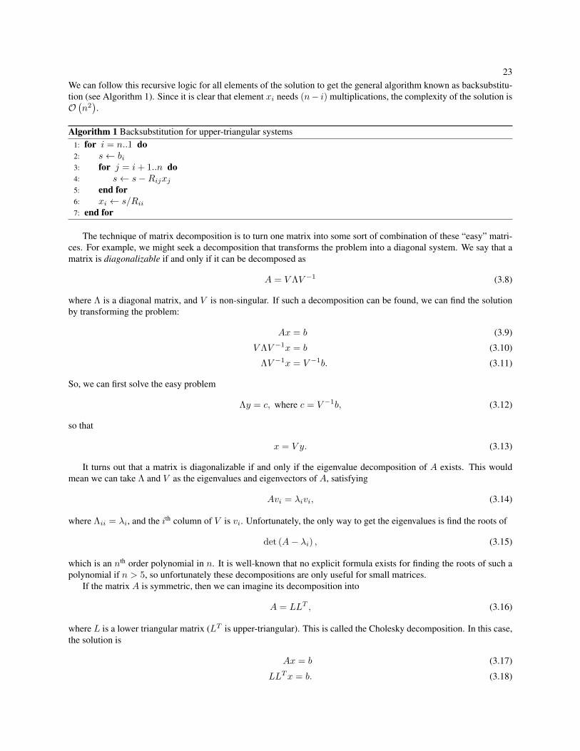
23We can follow this recursive logic for all elements of the solution to get the general algorithm known as backsubstitu-tion (see Algorithm 1). Since it is clear that element xi needs (n− i) multiplications, the complexity of the solution isO(n2).

Algorithm 1 Backsubstitution for upper-triangular systems1: for i = n..1 do2: s← bi3: for j = i+ 1..n do4: s← s−Rijxj5: end for6: xi ← s/Rii7: end for

The technique of matrix decomposition is to turn one matrix into some sort of combination of these “easy” matri-ces. For example, we might seek a decomposition that transforms the problem into a diagonal system. We say that amatrix is diagonalizable if and only if it can be decomposed as

A = V ΛV −1 (3.8)

where Λ is a diagonal matrix, and V is non-singular. If such a decomposition can be found, we can find the solutionby transforming the problem:

Ax = b (3.9)

V ΛV −1x = b (3.10)

ΛV −1x = V −1b. (3.11)

So, we can first solve the easy problem

Λy = c, where c = V −1b, (3.12)

so that

x = V y. (3.13)

It turns out that a matrix is diagonalizable if and only if the eigenvalue decomposition of A exists. This wouldmean we can take Λ and V as the eigenvalues and eigenvectors of A, satisfying

Avi = λivi, (3.14)

where Λii = λi, and the ith column of V is vi. Unfortunately, the only way to get the eigenvalues is find the roots of

det (A− λi) , (3.15)

which is an nth order polynomial in n. It is well-known that no explicit formula exists for finding the roots of such apolynomial if n > 5, so unfortunately these decompositions are only useful for small matrices.

If the matrix A is symmetric, then we can imagine its decomposition into

A = LLT , (3.16)

where L is a lower triangular matrix (LT is upper-triangular). This is called the Cholesky decomposition. In this case,the solution is

Ax = b (3.17)

LLTx = b. (3.18)

24

Algorithm 2 Cholesky decomposition1: for j = 1..n do2: Ljj ← Ajj3: for k = 1..j − 1 do4: Ljj ← Ljj − L2

jk

5: end for6: Ljj ← L

12jj

7: for i = j + 1..n do8: Lij ← Aij9: for k = 1..j − 1 do

10: Lij ← Lij − LikLjk11: end for12: Lij ← Lij/Ljj13: end for14: end for

By letting y = LTx, we can first solve Ly = b using forward substitution, a variant of Algorithm 1, then solveLTx = y using Algorithm 1 in O

(n2)

time. By examining Algorithm 2, we can see the decomposition itself requiresj multiplications for element Lij , and summing over all j ≤ i ≤ n gives total complexity of O

(n3).

The QR decomposition uses a combination of a unitary matrix and a triangular matrix:

A = QR, (3.19)

where Q is unitary and R is upper-triangular. If we have such a decomposition, then it can be solved in the followingway.

Ax = b (3.20)QRx = b (3.21)

Rx = QT b. (3.22)

So, we can just solve Rx = c using Algorithm 1 in O(n2)

time where c = QT b.TheQR decomposition can be realized by the Gram-Schmidt procedure in which orthogonal vectors are generated

sequentially. With the procedure given in Algorithm 3, we see that each vector qi needs 2n(i− 1) multiplications, andsumming over all n vectors gives O

(n3)

as the total complexity. There are other algorithms utilizing Householderreflections [14] to obtain the decomposition that are more numerically stable.

Algorithm 3 Gram-Schmidt QR decomposition

1: A∆= [a1, . . . , an]

2: Q∆= [q1, . . . , qn]

3: q1 ← a1

4: q1 ← q1/ ‖q1‖5: for i = 2..n do6: qi ← ai7: for j = 1..i− 1 do8: qi ← qi − 〈qj , ai〉qj9: end for

10: qi ← qi/ ‖qi‖11: end for12: R← QTA

A slight modification to the eigenvalue decomposition makes the problem much easier. If we change the decom-

25position a bit such that

A = UΣV T (3.23)

for some diagonal Σ and unitary U and V , then

Ax = b (3.24)

UΣV Tx = b (3.25)

ΣV Tx = UT b. (3.26)

This is called the singular value decomposition (SVD). So, to get the solution, we can apply the same strategy as wedo for the eigenvalue decomposition:

Σy = c, where c = UT b, (3.27)

and then

x = V y. (3.28)

The procedure to construct the SVD is too long to include in algorithmic form here, but we state the result that it isO(n3)

complexity.So, in increasing order of complexity, the typical matrix decompositions and solving routines are

1. Diagonal matrices (O (n))

2. Unitary matrices (O(n2))

3. Triangular matrices (O(n3))

4. Cholesky, QR, and singular value decompositions (O(n3))

5. Eigenvalue decomposition (unclear, but usually O(n3)

in practice).

Since the QR and singular value decompositions apply to arbitrary matrices and can be performed in a numerically-stable manner, this suggests that solving dense matrix equations is fundamentally an O

(n3)

problem.This was the conventional wisdom for hundreds of years until [4] proved otherwise. They showed that matrix

inversion can be performed stably in O(nω+η) time if and only if the matrix multiplication can also be performedstably in O(nω+η) time. For these dense matrices, ω = 2 describes the O

(n2)

complexity of dense multiplication,and η = 0.376 is a small extra factor required for stability. The argument comes from their proof that under theassumptions, the QR decomposition is stably computed in O(nω+η) multiplications. Given that decomposition, theinversion as we showed above is simple.

3.2 Gradient DescentMatrix decomposition is a great technique for solving dense matrix equations. However, we encounter practicalproblems when the system is sparse. We say a linear system is sparse if the number of nonzeros of the system isO (n). The reason this creates trouble is because although a compressed representation of such a system may fitcomfortably in memory, the decomposition will be a full matrix (in general) and will tend to dominate the memoryusage as n becomes large.

When the size of a sparse system becomes large, we require techniques that do not require an explicit decom-position. Rather, we favor techniques that can give succesively better approximations to the solution: that is to sayiterative techniques. The general approach is to define some function that is smooth and that is minimized at thedesired solution. Then, we can apply results from linear and nonlinear optimization to approach the solution.

One of the most natural ways to write such an objective function is

f(x)∆= ‖Ax− b‖22 , (3.29)

26where ‖·‖2 is the Euclidean norm. If a unique solution exists, then f(x) is minimized at the point that satisfiesAx = b,since f(x) ≥ 0 for any x by the properties of the norm, and f(x) = 0 at the solution.

We can rewrite the objective in terms of inner products:

f(x) = 〈x,ATAx〉 − 2〈x,AT b〉+ 〈b, b〉. (3.30)

The gradient, which represents the direction of greatest instantaneous increase is then

∇f(x) = 2ATAx− 2AT b. (3.31)

Because we want to minimize this function, this suggests the simple scheme

xn∆= xn−1 − δn−1∇f(xn−1), (3.32)

where δn > 0 is some step size that may or may not depend on n. For a given method to choose δ and x0, we obtainan instantiation of gradient descent.

In our particular case for matting by graph Laplacian, A is positive semi-definite by construction, and we can getbetter stability by changing the objective function to

f(x)∆=

1

2〈x,Ax〉 − 〈x, b〉. (3.33)

Then, the gradient becomes

∇f(x) = Ax− b, (3.34)

which is zero only at the solution. This provides more numerical stability because the quadratic operator is now Ainstead of ATA, and if the condition number of ATA is κ2, then the condition number of A is κ. A natural choice forthe step size is one that minimizes xn minimizes f(x) along the descent direction. This is called steepest descent, andprovides

δn∆=〈rn, rn〉〈rn, Arn〉

, where (3.35)

rn∆= ∇f(xn). (3.36)

The algorithm is given in Algorithm 4.

Algorithm 4 Steepest descentx← x0

for i = 1..K dor ← Ax− bδ ← 〈r, r〉/〈r,Ar〉x← x− δr

end for

For a more rigorous analysis of the convergence of steepest descent, refer to [28] that the error reduction ratio isbounded by ∥∥eK∥∥

A

‖e0‖A≤(κ− 1

κ+ 1

)K, (3.37)

where κ is the condition number of A. If we require that the error reduction ratio∥∥eK∥∥A

‖e0‖A≤ ε, (3.38)

27then we can get a lower bound on the number of required iterations K:(

κ− 1

κ+ 1

)K≤ ε (3.39)

K log

(κ− 1

κ+ 1

)≤ log (ε) (3.40)

K log

(κ+ 1

κ− 1

)≥ log

(1

ε

)(3.41)

K log

(1 + 1/κ

1− 1/κ

)≥ log

(1

ε

)(3.42)

2K

(1

κ+

1

3κ3+ · · ·

)≥ log

(1

ε

). (3.43)

So, we can chooseK ≥ 0.5κ log(1/ε) to sufficiently reduce the error. Since the number of iterations required isO (κ),and Algorithm 4 requires O (n) multiplications per iteration if A is sparse, the total complexity for steepest descenton sparse matrices is O (nκ).

3.3 Conjugate Gradient DescentConjugate gradient descent (CG) [12] is a modification of gradient descent that attempts to remedy the cycling problemof gradient descent.

Let the notation

〈x, y〉A = 〈x,Ay〉, (3.44)

for a positive definite matrix A. We say that x and y are conjugate with respect to A iff. 〈x, y〉A = 0. Suppose that

P∆= pi ∀i ∈ [1, n] | 〈pi, pj〉A = 0 ∀i 6= j . (3.45)

That is, P is a complete set of mutually-conjugate vectors. We also write pi ⊥A pj to denote conjugacy. Since A > 0,P is also a basis for Rn.

Then, we can write

x =

n∑i=1

αipi, (3.46)

with each αi ∈ R, where Ax = b. Then,

b = Ax =

n∑i=1

αiApi. (3.47)

By choosing any pj ∈ P , we have

〈pj , b〉 =

n∑i=1

αi〈pj , Api〉 (3.48)

= αj〈pj , Apj〉, (3.49)

due to the conjugacy of P . We can then recover

αj =〈pj , b〉〈pj , pj〉A

. (3.50)

28

Algorithm 5 Conjugate gradient descentx← x0

r ← b−Axz ← rp← zfor i = 1..K do

α← 〈r, z〉/〈p, p〉Ax← x+ αAprnew ← r − αApznew ← rnew

β ← 〈znew, rnew〉/〈z, r〉p← znew + βpz ← znew

r ← rnew

end for

It turns out that we can generate pi sequentially without significant effort, leading to Algorithm 5. Due to the factthat the iteration steps are along the pi and that they are mutually conjugate and span the entire space, it is a fact that(excepting numerical errors) the algorithm converges exactly to x in at most n iterations.

If A is dense, then each iteration has O(n2)

multiplications. Since we have to perform K = n iterations in theworst case, this gives an overall worst-case complexity of O

(n3)

for dense matrices, and by the same logic O(n2)

for sparse systems.For a more rigorous analysis of the convergence of CG, refer to [28] that the error reduction ratio is bounded by∥∥eK∥∥

A

‖e0‖A≤ 2

(√κ− 1√κ+ 1

)K, (3.51)

where κ is the condition number of A. If we require that the error reduction ratio∥∥eK∥∥A

‖e0‖A≤ ε, (3.52)

then we can get a lower bound on the number of required iterations K:

2

(√κ− 1√κ+ 1

)K≤ ε (3.53)

K log

(√κ− 1√κ+ 1

)≤ log

( ε2

)(3.54)

K log

(√κ+ 1√κ− 1

)≥ log

(2

ε

)(3.55)

K log

(1 + 1/

√κ

1− 1/√κ

)≥ log

(2

ε

)(3.56)

2K

(1√κ

+1

3√κ

3 + · · ·

)≥ log

(2

ε

). (3.57)

So, we can choose K ≥√κ/2 log(2/ε) to sufficiently reduce the error. Since the number of iterations required is

O (√κ), the total complexity for CG on sparse matrices is O (n

√κ), a significant improvement from the O (nκ) of

steepest descent.

29

Table 3.1: Comparison of solvers on the matting problemAlgorithm Space Time

Complete Factorization O(n3)O(n3)

Steepest Descent O (n) O (nκ) = O(n2)

CG O (n) O (n√κ) = O

(n1.5

)3.4 PreconditioningPreconditioning is a general framework that describes a way to reduce the number of iterations required in iterativeschemes by implicitly estimating the inverse of the system. The idea is to find a matrix T to modify the problem suchthat

TAx = Tb. (3.58)

If T is chosen such that κ(TA) κ(A), then iterative schemes applied to this new system will converge faster.One choice for sparse positive definite matrices is the incomplete Cholesky factorization. If we had a Cholesky

factorization A = LLT , then we could construct T = A−1 and solve the problem in a single iteration. However, theCholesky factorization is dense and unsuitable to store for large sparse matrices. The incomplete Cholesky factoriza-tion attempts to create a sparse matrix K that is similar to the dense factorization L. A simple way to create K is toperform the Cholesky decomposition, but to set Kij to zero if Aij is zero. This procedure is given in Algorithm 6.Then, the preconditioner T =

(KKT

)−1can be applied to reduce the condition number and the required number of

iterations. This is especialy popular to use with the conjugate gradient to obtain preconditioned conjugate gradientmethod [15].

Algorithm 6 Incomplete Cholesky decomposition1: for j = 1..n do2: Kjj ← Ajj3: for k = 1..j − 1 do4: Kjj ← Kjj −K2

jk

5: end for6: Kjj ← K

12jj

7: for i = j + 1..n do8: if Aij 6= 0 then9: Kij ← Aij

10: for k = 1..j − 1 do11: Kij ← Kij −KikKjk

12: end for13: Kij ← Kij/Kjj

14: end if15: end for16: end for

3.5 Applications to MattingIn the existing literature, the previous solution methods are used in various fashions. Since the iterative methods havecomplexity dependent on the condition number, we need to estimate that in order to get a clear picture of the practicalcomplexity. Since the matting Laplacian defines a second-order elliptic PDE, our system tends to have a conditionnumber κ ∈ O

(n

2d

), where d is the spatial dimensionality, which is 2 in this case [28]. So, we can substitute n for κ

in the complexity analyses to obtain Table 3.1.

30Because all the methods summarized in Table 3.1 are not scalable as the resolution n grows, they are usually not

used directly in practice. Some of the matting methods modify the previous algorithms directly, some use heuristicsto simplify the solution, and some modify or decompose the input first.

In [30], the matting Laplacian is fixed across all instances of the problem to be the spatial Laplace operator.Although there are specialized efficient methods to solve with this operator, the work instead chooses to use successiveover-relaxation (SOR), which is a straightforward iterative method that we will describe later. Since their method doesnot have a fixed right-hand side, they iterate between the SOR stage and recomputing the right-hand side.

In [19], the matting Laplacian is data-dependent. For small images, they say they use the “backslash” operator inMATLAB, which amounts to a Cholesky decomposition in this case. To deal with larger images, they downsampleto a small resolution, solve in the same manner, then do interpolation and thresholding to get back to full resolution.They mention briefly that they implemented a multigrid solver to handle large problems, but give no details and statethat it degrades the quality.

[11] use the conjugate gradient method. To work on large images, they split the problem into axis-aligned rect-angles that contain both foreground and background constraints. They then solve for the matte in each segmentindependently.

31

Part II

My Work

32

Chapter 4

Addressing Quality & User Input

Quality and the amount of user input required to get that quality are two fundamental concerns of natural imagematting. Below, we describe our works [16] and [17] that make progress on both fronts.

4.1 L1 MattingMany matting problems are formulated as minimization problems, where the objective function contains a term pro-portional to the energy encoded by the image and the matte. In other words, we often see problems formulated underL2 as

αΩ = arg minα

∫Ω

|T [I]− α|2 dx (4.1)

where T [I] is some transformation applied to the image, and Ω is small enough such that the matte is expected to beroughly constant there. If there is little interaction between alpha values on different domains, then it is clear that theoptimum solution for alpha over each domain is the mean of T [I].

In closed-form matting, the terms of the objective function are∑i∈wj

|αi − ajIi − bj |2 , (4.2)

and in poisson matting, the objective function is

αΩ = arg minα

∫Ω

∣∣∣∣ 1

F −B∇I −∇α

∣∣∣∣2 dx. (4.3)

Such formulations utilizing the L2 norm have some nice statistical properties and solutions. However, there is littlereason to assume that the L2 norm is the “right” norm. The mean that is associated with this norm also has drawbacks.It can be very sensitive to noise and outliers in some areas, and causes oversmoothing in other areas.

In our approach, we consider the usefulness of the L1 norm. It turns out to be that the median filtered image Ψ[I]plays a crucial role in L1. Specifically, it is much smoother over foreground and background regions, but in contrastwith the mean intrinsic to L2 space, it tends to preserve information on the edges between foreground and background.The L2 interpretation of this L1 feature is that it forces foreground and background to be smooth. This leads to theintriguing conclusion that it is not always necessary to completely reformulate methods from L2 to L1 to utilize thebenefits of L1 space.

To illustrate this idea, we reformulate a the well-known method of closed-form matting. Since the local estimate ofthe matte depends directly on the image data, there are often patches within the result that exhibit too much fluctuationunless the smoothing parameter ε is chosen large enough, in which case the boundaries can become overly smooth.By letting the matte depend on the L1 data Ψ[I] instead, we improve the quality of the homogeneous regions of thematte without sacrificing as much of the quality along the boundaries. We show direct comparisons between the twomethods in the mattes of blurred objects and static objects, and provide numerical evidence that our method generatesbetter mattes.

33We posit that matting using the median-filtered image Ψ[I] in place of the image itself generally provides better

results. The median filter is a non-linear filter that tends to preserve edges in an image while making the other regionsmore uniform. Techniques such as closed-form and Poisson matting make the assumption that the foreground andbackground images are smooth. But for most natural images, there is no reason to assume that they are, since thereis no natural phenomenon that causes physical objects to be band-limited. This makes such assumptions troublesome.However, by using Ψ[I] instead, we smooth out the foreground and background in the appropriate places and bettersatisfy the assumption, without compromising the information carried by edges.

4.1.1 MethodsBefore we consider the L1 norm and its usefulness toward matting, we first need to define the median. Take Ω to be adomain in Rn with finite Lebesgue measure and f ∈ C(Ω) ∩ L1(Ω) to be a real-valued function on Ω. According toa theorem of [24], there exists a unique m∗ ∈ R where

M(m) :=

∫Ω

|f(x)−m| dλn(x) (4.4)

is minimized. We call m∗ the median of f over Ω with respect to λn.The typical minimization problem under L1 gives us

αΩ = arg min∫

Ω

|T [I]− α| dx (4.5)

which we now recognize as the median of T [I] according to equation (4.4). The median, in contrast with the mean,resolves the issue of noise sensitivity. It also does not cause oversmoothing issues near sharp edges, where most of theperceptual information is located.

Now we explain the concept of L1 matting in an intuitive sense. For most of the image, α should be nearly constantand either 0 or 1. This means that even though Ψ is non-linear,

Ψ[I] ≈ αΨ[F ] + (1− α)Ψ[B] (4.6)

except near transition regions. And of course, Ψ[F ] and Ψ[B] are smoother than F and B. But near the transitionregions, we have

Ψ[I] ≈ I = αF + (1− α)B. (4.7)

What equations (4.6) and (4.7) mean, is that if we are concerned only with Ψ[I], we eliminate the need for smoothnessassumptions on F and B for the large majority of the image. Another interpretation is that we force the smoothnessassumption to be true in regions that are clearly foreground or background.

Interestingly, in many cases it seems unnecessary to reformulate the whole problem to L1 to take advantage of Ψ.As an example, we modify the closed-form approach. Notice that the individual terms of the objective function are ofthe form ∑

i∈wj

|αi − ajIi − bj |2 . (4.8)

If we use the L1 norm instead of L2, we do not lose the meaning of the cost function, since its use is only to make thesolution easier to obtain. Taking wj sufficiently small, αi ≈ αj ∀i ∈ wj . So if we make these changes,

α∗ := arg min∑i∈wj

|α− ajIi − bj | (4.9)

which is nothing but a discrete version of equation (4.4). In other words, α∗ = Ψ[ajIi − bj ], or

αi ≈ ajΨ[I]i + bj ∀i ∈ wj . (4.10)

However, care must be taken when considering the radius of Ψ. Any feature with a thickness smaller than theradius will be obliterated. This can be a problem for images with fine structures (such as hair) near transition regions.However, one way around this is to introduce a second operator which preserves these structures. In other words:

34

αi ≈ ajΨr1 [I]i + bjΨr2 [I]i + cj ∀i ∈ wj , (4.11)

where r1 is the radius of Ψ chosen to be smaller than the width of the finest structures, and r2 is a radius chosento sufficiently smooth the interior regions. S := Ψr1 [I] and L := Ψr2 [I]. The closed-form objective function thenbecomes:

J(α,a,b, c) :=

1

2

∑j∈I

∑i∈wj

(αi − ajSi − bjLi − cj)2 + ε1a2j + ε2b

2j

.(4.12)

The ratio ε1/ε2 should be chosen high enough to preserve the small features, but not so large as to destroy the smooth-ness of interior regions, and both should be small enough to prevent global over-smoothing.

Since J is composed of quadratic functions of linear combinations of the variables, it is convex. This structurealso means that the gradient components are linear in terms of the variables. For example,

∂J

∂αk= αk|wk| − Sk

∑j∈wk

aj − Lk∑j∈wk

bj −∑j∈wk

cj , (4.13)

and in vector notation,

∂J

∂αk=[0, . . . , |wk|, 0, . . . ,

0, . . . ,−Sk,−Sk, . . . ,0, . . . ,−Lk,−Lk, . . . ,0, . . . ,−1,−1, . . . , 0, . . .]x,

(4.14)

if x := [α,a,b, c]T .So, the unconstrained problem can be solved exactly by a sparse set of linear equations given by

∂

∂xkJ = Ak · x = 0 if xk unconstrained

Ak · x = ek · x = vk if xk constrained to be vk

where Ak is the kth row of matrix A ∈ R4n × R4n.We have implemented this matrix method in Matlab and have been using it when the number of pixels is relatively

small. However, notice that the number of non-zero entries is O(n). Therefore, the time complexity of the algorithmis O(n2), which is quite steep for images as the resolution grows.

To get the solution more efficiently, it is worth noting that a well-constructed iterative gradient descent methodwill terminate exactly on the optimal solution in 4n iterations or less (excepting round-off errors). Therefore, gradientdescent has a much better complexity of O(n). Each iteration of the descent forms the next estimate xp+1 by xp+1 =xp − λ∇J(xp), where λ is the step size that minimizes J(xp − λ∇J(xp)). Since this is a 1-d minimization over λ,we can find it easily, and the solution is

λ =T1 − T2

T3 − T4, (4.15)

35

(a) A moving car and the input scribbles

(b) Closed-form result followed by our result

Figure 4.1: Notice the horizontal stripes begin to fade in our result.

where

T1 =∑j∈I

(ε1apj∇a

pj + ε2b

pj∇b

pj )

T2 =∑j∈I

∑i∈wj

(αpi − apjSi − b

pjLi − c

pj )

×(∇αpi −∇apjSi −∇b

pjLi −∇c

pj )

T3 =∑j∈I

(ε1(∇apj )2 + ε2(∇bpj )

2)

T4 =∑j∈I

∑i∈wj

(∇αpi −∇apjSi −∇b

pjLi −∇c

pj )

2

and∇apj is the component of∇J(xp) corresponding to aj , for example.The effect of our formulation as given by equation (4.12) is like an adaptive median filter. In interior regions, bj

should be larger that aj , meaning that the large-radius median filter is active. Near transition regions, aj should belarger than bj . This suggests another way to formulate the problem.

Instead of a fixed-radius Ψ, it should be possible to design an adaptive version which is cognizant of transitionregions. Perhaps this could be done using gradient information. This is something we will pursue in the near future.

4.1.2 Experiments & ResultsIn figure 4.1, we show the tail of a car that is travelling from left to right, leaving a motion blur. Giving the image tothe closed-form method produces the image in the lower left. Utilizing median information gives our result bottomright. Notice that not only have the horizontal stripes begun to fade, but the faint glow above the car has attenuatedas well. In general, the alpha matte in the foreground and background regions is smoother, without over-smoothing inthe transition region. The fact that we can achieve better results with motion-blurred images is quite significant, since

36

((a) A person’s face and the input scribbles

(b) Closed-form result followed by our result

(c) Background replacement

Figure 4.2: Pink hair is remedied.

37recovering the unblurred image depends on a high-quality alpha matte in some recent algorithms [3]. There are someartifacts near the edges and corners of the image, but they are only due to Matlab’s implementation of the median filter.

In figure 4.2, we show a typical portrait view of a person. The closed-form method result in the lower left cornergives errors near the edges of the hair and where the hair changes color quickly due to highlights, where the assumptionof smooth foreground fails. It also produces a bit of noise in the matte in the area between the hair and the left andright edges of the image. This means that some of the hair is assumed to be a bit transparent, which is obviously errant.In our result at the bottom right, the matte is much smoother over the hair, and does not show the same noise as inthe closed-form result. As a result, background replacement with closed-form matting makes the highlights in the hairappear pink, while ours stays truer to the original color.

For numerical comparison, we obtained 27 images along with their ground truth alpha mattes from [27]. We thencomputed the alpha mattes for both methods with constant parameters, and found the absolute error with respect tothe ground truth mattes. The parameters were chosen to give the least average error for each method, which meantε = 10−5 for closed-form matting, and r1 = 0.5, r2 = 2, ε1 = 10−5, ε2 = 10−5 for our method. The input givenwas a sparse trimap, meaning that 80% to 90% of the image is classified as unknown. The result of the experiment isthat the average error for our method is 93% of the closed-form error. Since the standard deviation for this figure wasonly 6.4%, we can say with over 99.99% confidence that using L1 information is more effective at generating accuratemattes given sparse trimaps. This means that our method could be more amenable to automatic generation of alphamattes, and we will pursue this in the near future.

4.2 Nonlocal MattingSo far, most papers on natural image matting have ignored one major question: what is good user input? In otherwords, what is the best input a user can provide so that the algorithm gives the most accurate results? To the best ofour knowledge, there is very little in the literature to answer: what is good input, and how can we provide the leastamount of input for the most accuracy? We answer these questions in [17] by showing that the nonlocal principle[1] acts as a very effective sparsity prior on the matte, and serves to dramatically reduce the human effort required togenerate an accurate matte. Using this technique, we can effectively handle textured regions, edges, and structure in away that no one has demonstrated before.

Suppose there is a subset of pixels that exactly cluster in the graph implied by Laplacian L, and that we constrainone of the pixels in that cluster to have alpha value a. Then, the value of the objective function αTLα is minimizedif the rest of the pixels in the cluster are also labeled a. The reason is that, if we have K clusters, αTLα can bedecomposed as

αTLα =

K∑k=1

∑(i,j)∈Ek

Aij(αi − αj)2, (4.16)

where Ek | k = 1, 2, . . . ,K is a partition of the edge set E. Therefore, labeling the rest of the values in the clusteras aminimizes αTLα. What this means is that if we can construct the affinities so that the graph clusters accurately onforeground and background objects, the user only needs to constrain a single pixel in each cluster, and the algorithmcan do the rest of the work.

In many cases, obtaining a good clustering is difficult by using Levin et al.’s Laplacian [19]. The main reason isthat there is an overly strong regularization of the problem with spatial patches. This causes many clusters to be smalland localized (Fig. 4.3.b). This may be fine for large smooth regions, but is inappropriate for textured regions. In anattempt to remedy this, Levin et al. presented another algorithm in [20] that combined the small clusters into largerones that they call matting components based on two priors: the components are heavily biased to be binary-valued,and they do not overlap. Their solution is a nonlinear optimization procedure with a non-convex and non-differentiableobjective function.

4.2.1 MethodsIn [17], we present a new approach that achieves better results directly. This new approach defines a new Laplacianbased on the nonlocal principle. The nonlocal principle [1] essentially states that given an image I , the denoised pixel

38

(a) (b) (c)

Figure 4.3: (a) Input image. (b) Labels after clustering Levin’s Laplacian. (c) Clustering nonlocal Laplacian.

i is a weighted sum of the pixels that have similar appearance, where the weights are given by some kernel k(i, j).More formally,

E [I(i)] ≈∑j

I(j)k(i, j)1

Di, where (4.17)

k(i, j)∆= exp

(− 1

h21

‖I(S(i))− I(S(j))‖2g −1

h22

d2(i, j)

)(4.18)

Di∆=∑j

k(i, j). (4.19)

Here, S(i) is a small spatial patch around pixel i, and d(i, j) is the pixel distance between pixels i and j. ‖·‖gindicates that the norm is weighted by point-spread function (PSF) g, which can be a center-weighted Gaussian PSFwith standard deviation on the order of the radius of spatial neighborhood S(i).

The nonlocal principle defines a discrete data distribution k(i, ·)/Di for each pixel i, and implies that the imagecan be sparsely represented by a few spatial patches. Suppose that, by analogy to Eq. (4.17), the alpha matte is suchthat

E [αi] ≈∑j

αjk(i, j)1

Di, (4.20)

or, we can write

Diαi ≈ k(i, ·)Tα, . (4.21)

39

(a) (b)

(c) (d)

Figure 4.4: (a) Nonlocal neighbors at pixel (5,29). (b) Spatial neighbors at pixel (5,29). (c) Nonlocal neighbors at(24,23). (d) Spatial neighbors at (24,23).

It then follows that

Dα ≈ Aα, where (4.22)

A =

k(1, 1) · · · k(1, N)...

k(N, 1) · · · k(N,N)

, and (4.23)

D =

D1 0. . .

0 DN

. (4.24)

Therefore, (D−A)α ≈ 0, and αT (D−A)T (D−A)α ≈ 0. What this means is that we can effectively have a mattingLaplacian based on the nonlocal principle Lc = (D −A)T (D −A).

Due to (4.23), our affinity includes texture information, has little spatial regularization, and is nonlinear. Further,since we expect sparsity from the nonlocal principle, Lc should exhibit the property of having a small number ofclusters for some permutation matrix P . For this reason, we refer to this Lc as the nonlocal clustering Laplacian.

To extract clusters from Lc, we adapt the method described in [23]. First, define

M =D−12 LcD

−12 . (4.25)

Then, calculate the m smallest eigenvectors of M (we take m = 10), V1, . . . , Vm. Now, we create a matrix U suchthat each column corresponds to an eigenvector, but normalized such that each row has unit length under the 2-norm.In this way, each pixel is associated with a type of feature vector with m components. Then, we can treat U as the datamatrix in the k-means clustering algorithm [9]. So, we use k-means to do the final segmentation to locate the clusters.Parameter k controls the final number of clusters and depends on the image complexity.

The key observation is that the number of clusters k that we need to describe the alpha matte is only on the orderof 10 to 20, even when the number of pixels is tens of thousands. According to the observation in (4.16), we only need

40

(a) (b) (c)

Figure 4.5: (a) Input image, pixel (76,49) highlighted in red. (b) Affinities to pixel (76,49) in [19] (c) Nonlocalaffinities to pixel (76,49).

the user to label k pixels in the entire image. This is in contrast to Levin et al.’s method, where their Laplacian doesnot cluster very well (Fig. 4.3), especially for small k, requiring dense user input in the form of large scribble regions,or even a nearly complete trimap.

To maintain accuracy of the matte near the edges, we present a modification to Levin et al.’s algorithm. First, somenotation. If C = τ1, . . . , τn, define α(C) to be a column vector of length n: [ατ1 , . . . , ατn ]

T . Unless otherwisespecified, vectors are column vectors. S(i) represents a spatial neighborhood of pixel i (patch), and N(i) representsthe nonlocal neighborhood of pixel i.

Suppose

Qα(N(i)) ≈ Q [X(N(i)),1]

[ββ0

](4.26)

∆=X0(N(i))

[ββ0

],

whereX is aN ×d vector of image features withN being the number of pixels, and d being the number of features orchannels (we use RGB or grayscale values), and Q = diag(k(i, ·)/Di), is a weighting matrix containing the nonlocaldata distribution. If we assume α is fixed, the optimal linear parameters are[

β∗

β∗0

]=

(XT

0 (N(i))QX0(N(i)) + λ

[Id 00 0

])−1

XT0 (N(i))Qα(N(i))

∆= X†0(i,Q, λ)α(N(i)). (4.27)

Here, λ is a small number (10−5 or so) whose purpose is to ensure that the eigenvalues of XT (N(i))QX(N(i)) arestrictly positive so that the pseudoinverse defined in equation (4.27) exists and is unique.

Since we now have

α(N(i)) ≈ X0(N(i))X†0(i,Q, λ)α(N(i)) (4.28)∆= Biα(N(i)), (4.29)

we can construct the quadratic form

αTLmα∆= q(α) (4.30)

=

N∑i=1

α(N(i))T (I−Bi)T (I−Bi)α(N(i)). (4.31)

41The difference from [19] is that their data matrices X0 are local, and weighted by a uniform data matrix Q = cI,while our data matrices are nonlocal, and appropriately weighted by the nonlocal kernel, biasing the solution towardour assumption (4.20), and inserting texture information into the algorithm.

To find α, we solve the following optimization:

α∗ = arg minα

q(α)

s.t. α(C) = k

where C is the set of user-constrained pixels and k is the vector of constrained values. This can be solved exactly andin closed form by a smaller quadratic program. Since we use this Laplacian Lm for matte extraction, we refer to it asthe nonlocal matting extraction Laplacian.

The result of this nonlocal modification is very important. First, by exploiting the nonlocal kernel, we utilizesome texture information on the image, effectively grouping pixels with similar texture. Second, the neighborhoodsused in calculating the Laplacian are essentially adaptively varying in size as shown in Fig. 4.4, removing the highlyspatial clustering effects of previous methods (see Fig. 4.3.b), and therefore reducing the amount of input needed.Another advantage is that the nonlocal neighborhoods can safely be much larger. The effect of large neighborhoodsis interpreted by [11] as a large point spread function on the matte, causing convergence of iterative solvers to greatlyspeed up. Conversely, if the pixel’s patch is not very similar to any other in the image, the nonlocal neighborhood willbe very small and convergence there will be slow. Therefore, an iterative solver can provide feedback to the user basedon the local convergence rates about the quality of the final matte, and where he or she should provide additional input.

4.2.2 Experiments & ResultsTo formally evaluate the algorithm we have developed, we test its accuracy on the dataset given by [27] by the meansquared error (MSE) as well as by visual inspection of matte quality. We use the algorithm in [19] for comparison,since it is the state of the art with respect to sparse user input. We provide it with the same user input as to ouralgorithm.

The results for the MSE are shown in Fig. 4.6, where we can immediately see a drastic reduction in MSE. In fact,the average ratio of the Levin’s MSE to the nonlocal MSE is 4.04 with a sample standard deviation of 1.0. Therefore,we can say that our method outperforms Levin’s with confidence > 99.99% when the input is sparse. Perhaps evenmore important is the observation that our MSE curve is much smoother, suggesting our method is more robust tovariations in user input.

However, the MSE does not have a linear correlation to human perception. So, we need to visually verify that theextracted mattes are high quality despite the sparse input. For this, we provide several examples in Fig. 4.7. First, itis obvious that the amount of input required for our method is miniscule. The effects of spatial regularization can beseen as oversmoothing in column (c), while our results in (d) remain crisp. In column (e), background replacementhighlights the limitations of [19], showing significant bleed-through, while ours in column (f) appears much cleaner.It is clear that even with such sparse input, the matte quality is much higher with our nonlocal matting.

42

Figure 4.6: MSE of Levin’s method vs. our method with the same amount of input on images from [27]. [19] = black,nonlocal = gray.

(a) (b) (c) (d) (e) (f)

Figure 4.7: Visual inspection of matte quality. (a) Input image. (b) Sparse user input. (c) Levin’s algorithm [19]. (d)Nonlocal algorithm. (e) Background replacement with (c). (f) Background replacement with (d).

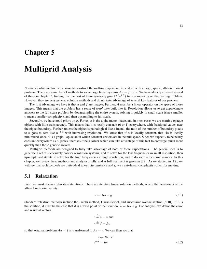
43

Chapter 5

Multigrid Analysis

No matter what method we choose to construct the matting Laplacian, we end up with a large, sparse, ill-conditionedproblem. There are a number of methods to solve large linear systems Au = f for u. We have already covered severalof these in chapter 3, finding that the best of these generally give O

(n1.5

)time complexity on the matting problem.

However, they are very generic solution methods and do not take advantage of several key features of our problem.The first advantage we have is that u and f are images. Further, A must be a linear operator on the space of those

images. This means that the problem has a sense of resolution built into it. Resolution allows us to get approximateanswers to the full scale problem by downsampling the entire system, solving it quickly in small scale (since smallern means smaller complexity), and then upsampling to full scale.

Secondly, we have good priors on u. For us, u is the alpha matte image, and in most cases we are matting opaqueobjects with little transparency. This means that u is nearly constant (0 or 1) everywhere, with fractional values nearthe object boundary. Further, unless the object is pathalogical like a fractal, the ratio of the number of boundary pixelsto n goes to zero like n−0.5 with increasing resolution. We know that if u is locally constant, that Au is locallyminimized since A is a graph Laplacian in which constant vectors are in the null space. Since we expect u to be nearlyconstant everywhere as n grows, there must be a solver which can take advantage of this fact to converge much morequickly than those generic solvers.

Multigrid methods are designed to fully take advantage of both of these expectations. The general idea is togenerate a set of succesively coarser resolution systems, and to solve for the low frequencies in small resolution, thenupsample and iterate to solve for the high frequencies in high resolution, and to do so in a recursive manner. In thischapter, we review these methods and analysis briefly, and A full treatment is given in [22]. As we studied in [18], wewill see that such methods are quite ideal in our circumstance and gives a sub-linear complexity solver for matting.

5.1 RelaxationFirst, we must discuss relaxation iterations. These are iterative linear solution methods, where the iteration is of theaffine fixed-point variety:

u← Ru+ g. (5.1)

Standard relaxtion methods include the Jacobi method, Gauss-Seidel, and successive over-relaxation (SOR). If u isthe solution, it must be the case that it is a fixed point of the iteration: u = Ru + g. For analysis, we define the errorand residual vectors

e∆= u− u and

r∆= f −Au

so that original problem Au = f is transformed to Ae = r. We can then see that

e← Re i.e.enew = Re (5.2)

44is the iteration with respect to the error. We can see that at the solution, u = u means that the error e = 0. It isimportant to realize that while r is the observable residual, e is unobservable in practice, obscured by requiring A−1.

Since we are concerned with how quickly the error converges to 0, it would be nice to say how much the erroris reduced in each iteration. The ratio ‖enew‖ / ‖e‖ captures the per-iteration error reduction and is what we call theconvergence rate.

From Equation 5.2, we can see that the convergence rate ‖enew‖ / ‖e‖ is bounded from above by the spectral radiusρ(R), since for any consist norm we have ‖Re‖ ≤ ‖R‖ ‖e‖, and ρ(R) ≤ ‖R‖. So, a simple upper bound for the errorreduction after j iterations is

∥∥ej∥∥ / ∥∥e1∥∥ ≤ ρ(R)j . For quickest convergence and smallest error, we obviously want

ρ(R) to be much less than 1.Recall ρ(R) = maxi

∣∣∣µi∣∣∣, where µi are the eigenvalues of R. So, to analyze the convergence, we need to under-stand the eigenvalues. Since e can be quite a complicated function in practice, it is useful to decompose the error e inthe basis of eigenvectors vi of R:

e1 =

n∑i=1

aivi. (5.3)

In other words, ai is the amount of spectral energy that e has at “frequency” i. We can think of it as frequency sincethe underlying graph is regular in structure, giving Eigenvectors that are increasingly oscillatory as i increases. This,this decomposition is very much a data-dependent version of the Fourier transform. Then, after j iterations, we cansee that

ej =

n∑i=1

µjiaivi. (5.4)

So, the closer µi is to zero, the faster the vi component of e converges to 0. For Laplace operators, ρ(R) = µ1, thelowest “frequency” Eigenvalue, and µ1 < 1 making the iteration always convergent.

Since µ1 is closest to 1, the v1 (low-frequency) component dominates the convergence rate, while the higher-frequency components are more easily damped out (for this reason, relaxation is often called smoothing). Further, weexplain that the convergence rate rapidly approaches 1 as n grows. To break this barrier, we need a technique that canhandle the low-frequencies just as well as the high frequencies.

5.2 Jacobi RelaxationA first attempt to solve Au = f is just to satisfy each equation independently:

ui(new) ← fi −Aiu, (5.5)

where Ai is the ith row of A. This is the strategy of the Jacobi Method. More completely, if D, −L, and −U are thediagonal, lower, and upper triangular parts of A resp., then A = D − L− U and the Jacobi Method is:

u← D−1(L+ U)u+D−1f. (5.6)

We can see that the relaxation matrix RJ = D−1(L + U). Since D is diagonal, it is trivial to invert and canbe done once and amortized over all the iterations. Further, RJ can be constructed in-place from A, and the onlyadditional storage required is a temporary vector u(new). Also advantageous is the fact that each element of u isupdated independently of all others, allowing trivial parallelization of the method. The only remaining question is howfast it converges.

In our case, RJ = D−1(L+U) is the normalized graph adjacency matrix D−1(AG), also called the random walkLaplacian. From well-known facts, its spectrum gives ρ(RJ) ≈ 1− c/n2 for some constant c. In order for the error tobe reduced to some tolerance τ , ∥∥ej∥∥ / ∥∥e0

∥∥ ≤ τ =⇒ (5.7)

(1− c/n2) ≤ τ =⇒ (5.8)

j ≈ n2− log(τ)

c∈ O

(n2). (5.9)

45

-1

-0.5

0

0.5

1

0 0.2 0.4 0.6 0.8 1

Jaco

bi Eig

envalu

es

Normalized Frequency

Figure 5.1: Jacobi method spectrum.

In fact, for typical Laplace operators on regular grids, common analysis gives

µi ≈ cos

(πi

n+ 1

), (5.10)

which plotted against normalized frequency (πi)/(n+1) gives Fig. 5.1. We can see that while the medium frequenciesconverge quickly, the low- and high-frequency errors converge very slowly.

5.3 Gauss-Seidel RelaxationGauss-Seidel is another relaxation method very similar to the Jacobi method. Instead of independently solving eachequation simultaneously, it attempts to do so sequentially. For example, it will update u1, then update u2 using thenew value of u1 it just computed. Unlike the Jacobi method, this means that it can be performed entirely in-place.

The Gauss-Seidel iteration can be described by

u← (D − L)−1Uu+ (D − L)−1f, (5.11)

so, the iteration matrix in this case is

RG = (D − L)−1U. (5.12)

Though we will not prove it here, it results that ρ(RG) ≤ [ρ(RJ)]2, meaning the convergence rate is half of the Jacobi

method, converging much more rapidly. In fact, the spectrum of RG typically gives µhi ≈ cos2(iπh), which is plottedin Figure 5.2. However, the cost of the increased performance is the loss of the ability to parallelize the scheme.

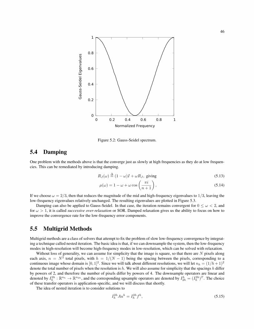
46

0

0.2

0.4

0.6

0.8

1

0 0.2 0.4 0.6 0.8 1

Gauss

-Seid

el Eig

envalu

es

Normalized Frequency

Figure 5.2: Gauss-Seidel spectrum.

5.4 DampingOne problem with the methods above is that the converge just as slowly at high frequencies as they do at low frequen-cies. This can be remediated by introducing damping.

RJ(ω)∆= (1− ω)I + ωRJ , giving (5.13)

µ(ω) = 1− ω + ω cos

(πi

n+ 1

), (5.14)

If we choose ω = 2/3, then that reduces the magnitude of the mid and high-frequency eigenvalues to 1/3, leaving thelow-frequency eigenvalues relatively unchanged. The resulting eigenvalues are plotted in Figure 5.3.

Damping can also be applied to Gauss-Seidel. In that case, the iteration remains convergent for 0 ≤ ω < 2, andfor ω > 1, it is called successive over-relaxation or SOR. Damped relaxation gives us the ability to focus on how toimprove the convergence rate for the low-frequency error components.

5.5 Multigrid MethodsMultigrid methods are a class of solvers that attempt to fix the problem of slow low-frequency convergence by integrat-ing a technique called nested iteration. The basic idea is that, if we can downsample the system, then the low-frequencymodes in high-resolution will become high-frequency modes in low-resolution, which can be solved with relaxation.

Without loss of generality, we can assume for simplicity that the image is square, so that there are N pixels alongeach axis, n = N2 total pixels, with h = 1/(N − 1) being the spacing between the pixels, corresponding to acontinuous image whose domain is [0, 1]2. Since we will talk about different resolutions, we will let nh = (1/h+ 1)2

denote the total number of pixels when the resolution is h. We will also assume for simplicity that the spacings h differby powers of 2, and therefore the number of pixels differ by powers of 4. The downsample operators are linear anddenoted by I2h

h : Rnh → Rn2h , and the corresponding upsample operators are denoted by Ih2h = (I2hh )T . The choice

of these transfer operators is application-specific, and we will discuss that shortly.The idea of nested iteration is to consider solutions to

I2hh Auh = I2h

h fh, (5.15)

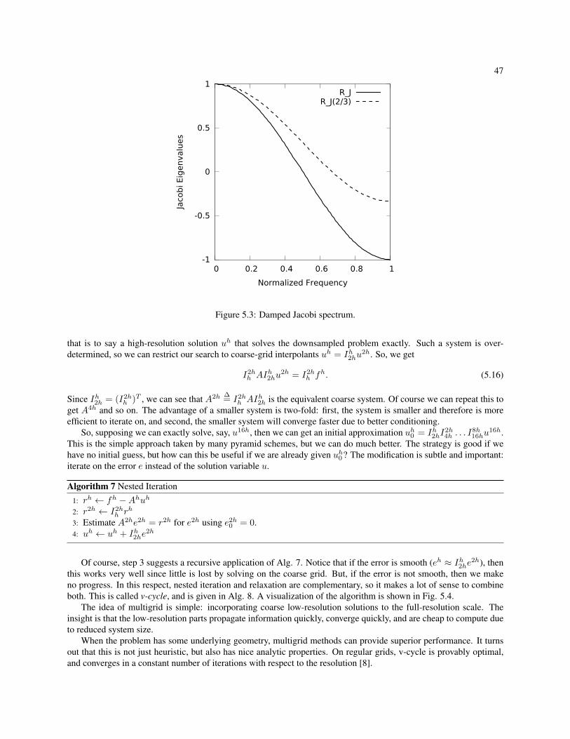
47

-1

-0.5

0

0.5

1

0 0.2 0.4 0.6 0.8 1

Jaco

bi Eig

envalu

es

Normalized Frequency

R_JR_J(2/3)

Figure 5.3: Damped Jacobi spectrum.

that is to say a high-resolution solution uh that solves the downsampled problem exactly. Such a system is over-determined, so we can restrict our search to coarse-grid interpolants uh = Ih2hu

2h. So, we get

I2hh AIh2hu

2h = I2hh fh. (5.16)

Since Ih2h = (I2hh )T , we can see that A2h ∆

= I2hh AIh2h is the equivalent coarse system. Of course we can repeat this to

get A4h and so on. The advantage of a smaller system is two-fold: first, the system is smaller and therefore is moreefficient to iterate on, and second, the smaller system will converge faster due to better conditioning.

So, supposing we can exactly solve, say, u16h, then we can get an initial approximation uh0 = Ih2hI2h4h . . . I

8h16hu

16h.This is the simple approach taken by many pyramid schemes, but we can do much better. The strategy is good if wehave no initial guess, but how can this be useful if we are already given uh0 ? The modification is subtle and important:iterate on the error e instead of the solution variable u.

Algorithm 7 Nested Iteration1: rh ← fh −Ahuh2: r2h ← I2h

h rh

3: Estimate A2he2h = r2h for e2h using e2h0 = 0.

4: uh ← uh + Ih2he2h

Of course, step 3 suggests a recursive application of Alg. 7. Notice that if the error is smooth (eh ≈ Ih2he2h), thenthis works very well since little is lost by solving on the coarse grid. But, if the error is not smooth, then we makeno progress. In this respect, nested iteration and relaxation are complementary, so it makes a lot of sense to combineboth. This is called v-cycle, and is given in Alg. 8. A visualization of the algorithm is shown in Fig. 5.4.

The idea of multigrid is simple: incorporating coarse low-resolution solutions to the full-resolution scale. Theinsight is that the low-resolution parts propagate information quickly, converge quickly, and are cheap to compute dueto reduced system size.

When the problem has some underlying geometry, multigrid methods can provide superior performance. It turnsout that this is not just heuristic, but also has nice analytic properties. On regular grids, v-cycle is provably optimal,and converges in a constant number of iterations with respect to the resolution [8].

48

Algorithm 8 V-Cycle1: function VCYCLE(uh,fh)2: if h = H then return exact solution uh

3: end if4: Relax on Ahuh = fh

5: rh ← fh −Ahuh (compute residual)6: e2h ← VCYCLE(e2h = 0,I2h

h rh) (estimate correction)7: uh ← uh + Ih2he

2h. (apply correction)8: Relax on Ahuh = fh

9: return uh10: end function

h

2h

4h

8h

r2h

r4h

r8h e8h

e4h

e2h

Figure 5.4: Visualization of the v-cycle schedule. The V shape is the reason for the name.

It is also important to see that the amount of work done per iteration is O (n) in the number of variables. To seethis, we can take relaxation on the highest resolution to be 1 unit of work. Looking at Alg. 8, there is one relaxationcall, followed by recursion, followed by another relaxation call. In our case, the recursion operates on a problem at 1/4size, so we have the total work asW (n) = 1+W (n4 )+1 = 2+W (n4 ). In general, the relaxation costs nh/N , and theexpression becomesW (nh) = 2nh

n +W (nh

4 ). If we continue the expression,W (n) = 2+2 14+2 1

16+· · · = 2∑∞i=0

14

n,which converges to W (n) = 8/3. In other words, the work done for v-cycle is just a constant factor of the work doneon a single iteration of the relaxation at full resolution. Since the relaxation methods chosen are usually O (n), then asingle iteration of v-cycle is also O (n). So, we get a lot of performance without sacrificing complexity.

V-cycle (and the similar w-cycle) multigrid methods work well when the problem has a regular geometry thatallows construction of simple transfer operators. When the geometry becomes irregular, the transfer operators mustalso adapt to preserve the performance benefits. When the geometry is completely unknown or not present, algebraicmultigrid algorithms can be useful, which attempt to automatically construct problem-specific operators, giving a kindof “black box” solver.

5.6 Multigrid (Conjugate) Gradient DescentHere, we describe a relatively new type of multigrid solver from [26] that extends multigrid methods to gradient andconjugate gradient descent. Please note that our notation changes here to match that of [26] and to generalize thenotion of resolution.

If the solution space has a notion of resolution on ` total levels, with downsample operators Ii` : Rn` → Rni , andupsample operators I`i : Rni → Rn` (ni < n` ∀i < `), then define the multi-level residuum space on xk at the kth

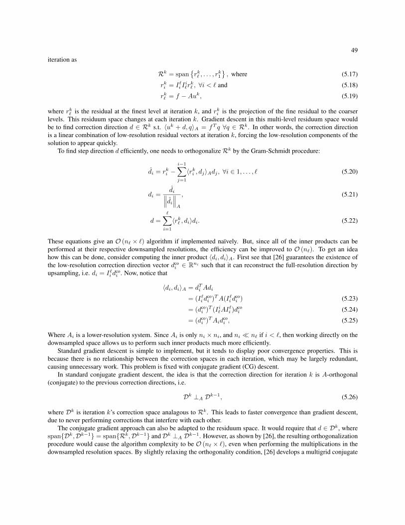
49iteration as

Rk = spanrk` , . . . , r

k1

, where (5.17)

rki = I`i Ii`rk` , ∀i < ` and (5.18)

rk` = f −Auk, (5.19)

where rk` is the residual at the finest level at iteration k, and rki is the projection of the fine residual to the coarserlevels. This residuum space changes at each iteration k. Gradient descent in this multi-level residuum space wouldbe to find correction direction d ∈ Rk s.t. 〈uk + d, q〉A = fT q ∀q ∈ Rk. In other words, the correction directionis a linear combination of low-resolution residual vectors at iteration k, forcing the low-resolution components of thesolution to appear quickly.

To find step direction d efficiently, one needs to orthogonalizeRk by the Gram-Schmidt procedure:

di = rki −i−1∑j=1

〈rki , dj〉Adj , ∀i ∈ 1, . . . , ` (5.20)

di =di∥∥∥di∥∥∥

A

, (5.21)

d =∑i=1

〈rk` , di〉di. (5.22)

These equations give an O (n` × `) algorithm if implemented naıvely. But, since all of the inner products can beperformed at their respective downsampled resolutions, the efficiency can be improved to O (n`). To get an ideahow this can be done, consider computing the inner product 〈di, di〉A. First see that [26] guarantees the existence ofthe low-resolution correction direction vector dco

i ∈ Rni such that it can reconstruct the full-resolution direction byupsampling, i.e. di = I`i d

coi . Now, notice that

〈di, di〉A = dTi Adi

= (I`i dcoi )TA(I`i d

coi ) (5.23)

= (dcoi )T (Ii`AI

`i )d

coi (5.24)

= (dcoi )TAid

coi , (5.25)

Where Ai is a lower-resolution system. Since Ai is only ni × ni, and ni n` if i < `, then working directly on thedownsampled space allows us to perform such inner products much more efficiently.

Standard gradient descent is simple to implement, but it tends to display poor convergence properties. This isbecause there is no relationship between the correction spaces in each iteration, which may be largely redundant,causing unnecessary work. This problem is fixed with conjugate gradient (CG) descent.

In standard conjugate gradient descent, the idea is that the correction direction for iteration k is A-orthogonal(conjugate) to the previous correction directions, i.e.

Dk ⊥A Dk−1, (5.26)

where Dk is iteration k’s correction space analagous to Rk. This leads to faster convergence than gradient descent,due to never performing corrections that interfere with each other.

The conjugate gradient approach can also be adapted to the residuum space. It would require that d ∈ Dk, wherespanDk,Dk−1 = spanRk,Dk−1 andDk ⊥A Dk−1. However, as shown by [26], the resulting orthogonalizationprocedure would cause the algorithm complexity to be O (n` × `), even when performing the multiplications in thedownsampled resolution spaces. By slightly relaxing the orthogonality condition, [26] develops a multigrid conjugate

50gradient (MGCG) algorithm with complexity O (n`).

Dk = spandk1 , . . . , d

kl

(5.27)∥∥dki ∥∥A = 1 ∀i ∈ 1, . . . , ` (5.28)

dki ⊥A dkj ∀i 6= j (5.29)

D1 = R1 (5.30)

dk−1i ⊥A dkj ∀k > 1, i ≤ j (5.31)

Rk +Dk−1 = Dk +Dk−1 (5.32)

We present Alg. 10, which fixes some algorithmic errors made in [26].

Algorithm 9 Multigrid gradient descent.1: while numIter > 0 do2: numIter ← numIter − 13: r` ← b−Ax4: d` ← r`5: for i = `− 1..1 do6: ri ← Iii+1ri+1

7: di ← ri8: end for9: for i = 1..` do

10: ki ← Aidi11: for j = i..2 do12: kj−1 ← Ij−1

j kj13: end for14: s1 = 0

15: for j = 1..i− 1 do16: sj ← sj + (kTj dj)dj

17: sj+1 ← Ij+1j sj

18: end for19: di ← di − si20: ki ← Aidi21: di ← di(k

Ti di)

− 12

22: end for23: s1 ← (dT1 r1)d1

24: for i = 2..` do25: si ← Iii−1si−1

26: si ← si + di27: end for28: x← x+ s`29: end while

In multigrid algorithms such as these, we have freedom to construct the transfer operators. If we want to takefull advantage of such algorithms, we must take into account our prior knowledge of the solution when designing theoperators.

51

Algorithm 10 Multigrid CG descent.1: Do one iteration of multigrid gradient descent.2: while numIter > 0 do3: numIter ← numIter − 14: r` ← b−Ax5: dnew

` ← r`6: for i = `− 1..1 do7: ri ← Iii+1ri+1

8: dnewi ← ri

9: end for10: for i = 1..` do11: ki ← Aidi12: for j = i..2 do13: kj−1 ← Ij−1

j kj14: end for15: s1 = 016: for j = 1..i− 1 do17: sj ← sj + (kTj d

newj )dnew

j

18: sj+1 ← Ij+1j sj

19: end for20: di ← di − si21: ki ← Aidi22: di ← di(k

Ti di)

− 12

23: ki ← Aidnewi

24: for j = i..2 do25: kj−1 ← Ij−1

j kj26: end for

52

27: s1 ← 028: for j = 1..i− 1 do29: sj ← sj + dnew

j (kTj dnewj )

30: sj ← sj + dj(kTj d

newj )

31: sj+1 ← Ij+1j sj

32: end for33: dnew

i ← dnewi − si

34: si ← dnewi − di(kTi di)

35: if ‖si‖∞ > ε ‖dnewi ‖∞ then

36: dnewi ← si

37: else38: dnew

i ← di39: di ← 040: end if41: ki ← Aid

newi

42: dnewi ← dnew

i (kTi dnewi )−1/2

43: end for44: d1 ← dnew

1

45: s1 ← d1(dT1 r1)46: for i = 2..` do47: di ← dnew

i

48: si ← Iii−1si−1

49: si ← si + di(dTi ri)

50: end for51: x← x+ s`52: end while

5.7 Evaluated Solution Methods

5.7.1 Conjugate GradientCG and variants thereof are commonly used to solve the matting problem, so we examine the properties of the classicCG method alongside the multigrid methods.

5.7.2 V-cycleIn order to construct a v-cycle algorithm, we need to choose a relaxation method and construct transfer operators. Wechose Gauss-Seidel as the relaxation method, since it is both simple and efficient. Through experiment, we found thatsimple bilinear transfer operators (also called full-weighting) work very well for the matting problem. The downsampleoperator I2h

h is represented by the stencil 116

18

116

18

14

18

116

18

116

.If the stencil is centered on a fine grid point, then the numbers represent the contribution of the 9 fine grid points totheir corresponding coarse grid point. The corresponding upsample operator Ih2h is represented by the stencil 1

412

14

12 1 1

214

12

14

.This stencil is imagined to be centered on a fine grid point, and its numbers represent the contribution of the corre-sponding coarse grid value to the 9 fine grid points. The algorithm is then given by Alg. 8.

53

20 40 60 80 100 120 140 160 180 20010−14

10−12

10−10

10−8

10−6

10−4

10−2

100

Iteration

Res

idua

l

Convergence at 4 Mpx

CGMGCGv−cycle

Figure 5.5: Convergence on a 4 Mpx image. Horizontal line denotes proposed termination value of 10−4.

Resolution CG MGCG v-cycle0.5 Mpx 0.594 0.628 0.019

1 Mpx 0.357 0.430 0.0172 Mpx 0.325 0.725 0.0174 Mpx 0.314 0.385 0.015

Table 5.1: Initial convergence rates ρ0 on image 5 in [27]. Lower is better.

5.7.3 Multigrid Conjugate GradientWe also examine the multigrid conjugate gradient algorithm of [26], which is a more recent multigrid variant, andseems like a natural extension of CG. For this algorithm, we find that the bilinear (full-weighting) transfer operatorsalso work very well. The algorithm is given by Alg. 10, where we give the full pseudo-code as the original pseudo-codegiven in [26] is erroneous.

5.8 Experiments & ResultsIn order to compare the solution methods, we choose the matting Laplacian proposed by [19], as it is popular andprovides source code. Please note that we are comparing the solvers, and not the performance of the matting Laplacianitself, as these solvers would equally apply to other matting Laplacians. We set their ε parameter to 10−3, and we formour linear system according to Eq. (1.6) with γ = 1.

All methods are given the initial guess α0 = 0. To make the objective value comparable across methods andresolutions, we take ‖f −Aαi‖2 / ‖f −Aα0‖2 = ‖f −Aαi‖2 / ‖f‖2 as the normalized residual at iteration i, orresidual for short. We set the termination condition for all methods at all resolutions to be the descent of the residualbelow 10−4.

First, we evaluate the convergence of conjugate gradient, multigrid conjugate gradient, and v-cycle. Typical be-

54

0 100 200 300 400 500 600 70010−14

10−12

10−10

10−8

10−6

10−4

10−2

100

Iteration

Res

idua

l

CG Convergence w.r.t. Resolution

0.5 Mpx1 Mpx2 Mpx4 Mpx

(a)

0 100 200 300 400 500 600 70010−15

10−10

10−5

100 MGCG Convergence w.r.t. Resolution

Iteration

Res

idua

l

0.5 Mpx1 Mpx2 Mpx4 Mpx

(b)

0 100 200 300 400 500 600 70010−15

10−10

10−5

100

Iteration

Res

idua

l

V−cycle Convergence w.r.t. Resolution

0.5 Mpx1 Mpx2 Mpx4 Mpx

(c)

Figure 5.6: CG (a) & MGCG (b) slow down as resolution increases, while v-cycle (c) speeds up.

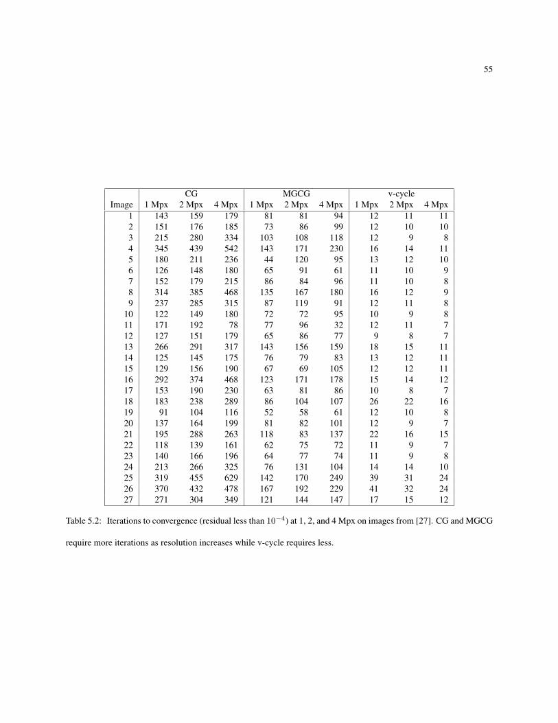
55

CG MGCG v-cycleImage 1 Mpx 2 Mpx 4 Mpx 1 Mpx 2 Mpx 4 Mpx 1 Mpx 2 Mpx 4 Mpx

1 143 159 179 81 81 94 12 11 112 151 176 185 73 86 99 12 10 103 215 280 334 103 108 118 12 9 84 345 439 542 143 171 230 16 14 115 180 211 236 44 120 95 13 12 106 126 148 180 65 91 61 11 10 97 152 179 215 86 84 96 11 10 88 314 385 468 135 167 180 16 12 99 237 285 315 87 119 91 12 11 8

10 122 149 180 72 72 95 10 9 811 171 192 78 77 96 32 12 11 712 127 151 179 65 86 77 9 8 713 266 291 317 143 156 159 18 15 1114 125 145 175 76 79 83 13 12 1115 129 156 190 67 69 105 12 12 1116 292 374 468 123 171 178 15 14 1217 153 190 230 63 81 86 10 8 718 183 238 289 86 104 107 26 22 1619 91 104 116 52 58 61 12 10 820 137 164 199 81 82 101 12 9 721 195 288 263 118 83 137 22 16 1522 118 139 161 62 75 72 11 9 723 140 166 196 64 77 74 11 9 824 213 266 325 76 131 104 14 14 1025 319 455 629 142 170 249 39 31 2426 370 432 478 167 192 229 41 32 2427 271 304 349 121 144 147 17 15 12

Table 5.2: Iterations to convergence (residual less than 10−4) at 1, 2, and 4 Mpx on images from [27]. CG and MGCG

require more iterations as resolution increases while v-cycle requires less.

56

Image a p1 11.8 -0.0652 11.7 -0.1403 11.8 -0.3094 16.2 -0.2615 13.2 -0.1836 11.0 -0.1447 11.2 -0.2208 16.0 -0.4159 12.3 -0.270

10 10.0 -0.16011 12.5 -0.34312 9.02 -0.18013 18.2 -0.34014 13.0 -0.12015 12.2 -0.06116 15.2 -0.15617 9.90 -0.26518 26.4 -0.33319 12.1 -0.28920 12.0 -0.39421 21.4 -0.30022 11.1 -0.32123 10.9 -0.23624 14.6 -0.21625 39.1 -0.34726 41.2 -0.38127 17.2 -0.243

Table 5.3: Fitting of v-cycle required iterations to anp (power law), with n being problem size in Mpx. Average p is

E[p] = −0.248, meaning this solver is sublinear in n.

57

Method SAD MSE Gradient ConnectivityOurs 11.1 10.8 12.9 9.1[19] 14 13.9 14.5 6.4[11] 17 15.8 16.2 9.2

Table 5.4: Average rank in benchmark [27] on 11 Mar 2013 with respect to different error metrics.

havior on the dataset [27] is shown in Fig. 5.5 at 4 Mpx resolution. CG takes many iterations to converge, MGCGperforms somewhat better, and v-cycle performs best.

Next, we demonstrate in Fig. 5.6 that the number of iterations v-cycle requires to converge on the matting problemdoes not increase with the resolution. In fact, we discover that v-cycle requires fewer iterations as the resolutionincreases. This supports a sub-linear complexity of v-cycle on this problem in practice since each iteration is O (n).

We list a table of the convergence behavior of the algorithms on all images provided in the dataset in Table 5.2.This demonstrates that MGCG performs decently better than CG, and that v-cycle always requires few iterations asthe resolution increases. By fitting a power law to the required iterations in Table 5.3, we find the average number ofrequired v-cycle iterations is O

(n−0.248

). Since each iteration is O (n), this means that this is the first solver demon-

strated to have sublinear time complexity on the matting problem. Specifically, the time complexity is O(n0.752

)on

average. Theoretical guarantees [8] ensure that the worst case time complexity is O (n).Though surprising, the sub-linear behavior is quite understandable. Most objects to be matted are opaque with a

boundary isomorphic to a line segment. The interior and exterior of the object have completely constant α locally,which is very easy for v-cycle to handle at its lower levels, since that is where the low frequency portions of thesolution get solved. This leaves the boundary pixels get handled at the highest resolutions, since edges are high-frequency. These edge pixels contribute to the residual value, but since the ratio of boundary to non-boundary pixelsis O

(n−0.5

), tending to 0 with large n, the residual tends to decrease more rapidly per iteration as the resolution

increases as proportiontely more of the problem gets solved in lower resolution.Another way to view it is that there is a fixed amount of information present in the underlying image, and increasing

the number of pixels past some point does not really add any additional information. V-cycle is simply the firstalgorithm studied to exploit this fact by focusing its effort preferentially on the low resolution parts of the solution.

Perhaps if we had enough computational resources and a high-enough resolution, v-cycle could drop the residualto machine epsilon in a single iteration. At that point, we would again have a linear complexity solver, as we wouldalways have to do 1 iteration at O (n) cost. In any case, O (n) is worst case behavior as guaranteed by [8], which isstill much better than any solver proposed to date like [11] and [32] (which are at best O

(n2)). We would also like to

mention that the per-iteration work done by the proposed method is constant with respect to the number of unknowns,unlike most solvers including [11] and [32].

Table 5.1 lists the initial convergence rates ρ0 (the factor by which the residual is reduced per iteration). [8]guarantees that the convergence rate for v-cycle is at most O (1) and bounded away from 1. We discover that on thematting problem the convergence rate is sub-constant. Yet again, v-cycle dramatically overshadows other solvers.

Although a MATLAB implementation of [19] is available, we found it to use much more memory than we believeit should. We therefore developed our own implementation in C++ using efficient algorithms and data structures torun experiments at increasing resolution. Since there are 25 bands in the Laplacian, and 4 bytes per floating pointentry, the storage required for the matrix in (1.6) is 95 MB/Mpx, and the total storage including the downsampledmatrices is about 127 MB/Mpx. The time to generate the Laplacian is 0.8 s/Mpx. The CPU implementation runs at46 Gauss-Seidel iterations/s/Mpx and 11 v-cycle iterations/s/Mpx. Assuming 10 iterations of v-cycle are run, whichis reasonable from Table 5.2, our solver runs in about 1.1 s/Mpx, which is nearly 5 times faster than [11] at lowresolutions, and even faster at higher resolutions. Upon acceptance of this paper, we will post all the code under anopen-source license.

Although we consider this to be a matting solver rather than a new matting algorithm, we still submitted it to theonline benchmark [27] using [19]’s Laplacian. The results presented in Table 5.4 show some improvement over thebase method [19], and more improvement over another fast method [11]. In theory, we should reach the exact samesolution as [19] in this experiment, so we believe any performance gain is due to a different choice of their ε parameter.

58

Chapter 6

Extensions to Image Formation

The methods we utilize in [18] are not limited to image matting. Those multigrid methods extend to a wide range ofproblems we refer to as image formation problems in Computer Vision and Image Processing. In general, if a problemhas the following characteristics, we can use multigrid methods to greatly enhance the efficiency:

1. Linear form Au = f , and A > 0

2. u is an image, or at least can be downsampled

3. A is large and sparse and κ(A)→∞ as n→∞

We investigate three such problems in our field, namely optical flow, image deconvolution, and texture modeling andsynthesis to show the utility of these methods in greatly reducing the computational cost that has heretofore beenassociated with them.

6.1 Optical FlowOptical flow is a classic Computer Vision problem. It asks for the displacement field for each pixel between twoframes of video. It starts by assuming that a pixel i retains its color after movement δi from frame t to frame t+ 1:

It+1(i+ δi) = It(i). (6.1)

Further, by assuming small displacement,

It+1(i+ δi) = It+1(i) + δTi ∇It+1(i) +O(‖δi‖2

)≈ It+1(i) + δTi ∇It+1(i). (6.2)

Then, we have

It(i) ≈ It+1(i) + δTi ∇It+1(i), or (6.3)

δTi ∇It+1(i) ≈ It(i)− It+1(i). (6.4)

Taken across all pixels i, and writing this in matrix notation:. . . 0 0

. . . 0 00 ∇uIt 0 0 ∇vIt 0

0 0. . . 0 0

. . .

n×2n

(δuδv

)2n×1

= It − It+1, or (6.5)

[Du Dv] δ = g (6.6)

59

1e-16

1e-14

1e-12

1e-10

1e-08

1e-06

0.0001

0.01

1

0 20 40 60 80 100 120

Resi

dual

Iteration

Horn-Schunck Optical Flow

CGV-cycle

Figure 6.1: V-cycle applied to optical flow.

Obviously, there are 2n variables in the vector field, but only n constraining equations. Solving this requires priorinformation on the field. Horn and Schunck [13] used a Laplace operator L as the regularizing term, since they expectthe motion field to be smooth. Also, to get the system to be square, we end up with([

D2u DuDv

DvDu D2v

]+ λ

[L 00 L

])δ =

[Du

Dv

]g

∆= f. (6.7)

Here, λ is a Lagrange parameter for the regularization on the smoothness of the motion field δ. Just as in matting, weend up with a large sparse system, whose variable represents something like an image.

1. X Linear form Au = f , and A > 0

2. X u is an image, or at least can be downsampled

3. X A is large and sparse and κ(A)→∞ as n→∞

This problem is perfectly-suited to be solved efficiently by multigrid algorithms. In fact, multigrid methods werestudied in the solution of optical flow in the 1980s [6], perhaps because multigrid methods were in their heyday at thesame time as optical flow made its mark. However, nobody ever analyzed the computational complexity. When weapply the same methods from [18] to Horn-Schunck optical flow, we get nearly the same results as before, and againobtain a sub-linear solver (Figure 6.1).

6.2 DeconvolutionDeconvolution is a fundamental issue in Image Processing. If an image gets filtered by some process, we may wish todeconvolve the noisy filtered image to get an approximation of the original. In other words

Hu = v, or (6.8)

HTHu = HT v, (6.9)

whereH is a convolutional matrix for the filter, u is the original image, and v is the filtered image. BecauseH is rarelyfull-rank, we need to regularize the system in some way to be able to recover u. A very simple way is to regularize the2-norm of u, since we do not expect solutions with very high energy:

(HTH + λI)u = HT v, (6.10)

60

Original Filtered

CG V-cycle

1e-16

1e-14

1e-12

1e-10

1e-08

1e-06

0.0001

0.01

1

0 10 20 30 40 50 60 70 80 90 100

Resi

dual

Iteration

Deconvolution

CGV-cycle

Figure 6.2: V-cycle on deconvolution

where again λ is the regularization parameter. IfH represents a sort of highpass kernel, we again have nearly the sameproblem as in Chapter 5, and we expect multigrid algorithms to give a large increase in performance.

1. X Linear form Au = f , and A > 0

2. X u is an image, or at least can be downsampled

3. X A is large and sparse and κ(A)→∞ as n→∞

6.3 Texture Modeling & SynthesisThere are two major veins of research about image textures. One concerns itself with describing or modeling thetexture, and the other concerns itself with synthesizing textures. The goal of modeling is more or less to provide aprior p(I | T ) over images I for a given type of texture T . The usefulness of such a prior is apparent in applicationslike super-resolution, where textured regions may be superresolved by matching low-resolution textures to a set ofhigh-resolution texture models. Texture synthesis is the opposite side of the coin, in which we ask to generate asample texture image from p(I | T ), whether or not we have such an explicit model.

These two approaches are unified in [34] in a very elegant way, in which a texture model is learned from examplesof the texture by creating an explicit Gibbs distribution, which is sampled using a Gibbs sampler in order to performthe learning. The result is an explicit form for p(I | T ) which can evaluate the likelihood of an image under the texturemodel, and can also generate new images. The disadvantage in both learning and synthesis is the reliance on the Gibbssampler.

The Gibbs sampler is a mechanism by which a Gibbs distribution (equivalently a Markov Random Field) can besampled by mariginalizing the distribution for a single pixel, drawing the pixel value from the marginal, and repeatingover all pixels in the image for a very large number of iterations until the distribution of the entire image convergesto that of the model. It is not at all clear how long or even if such an algorithm will converge, and in this particularcontext, it may be necessary to visit each pixel in the image hundreds or thousands of times before the generatedtexture can be said to be drawn from the model.

In practice, we observe for a fixed model, the complexity of generating a texture with n pixels is O (n). However,as the resolution of the learned texture increases, the model must incorporate features from larger and larger filters tocapture the large-scale structures. This means that in order to accurately learn and synthesize a texture with n pixels,

61

the total complexity is something likeO(n2). Since even small textures on a 128×128 grid can take hours to converge

on modern hardware, we need more efficient algorithms to make this type of modeling and synthesis practical.We propose importing and modifying the concepts of multigrid analysis to the Gibbs sampler in order to make

synthesis more efficient. First, let us look at the Gibbs sampling algorithm 11. Its inputs are the initial texture u, themarginal distributions p(v, i) = p (u(v) = i | u(−v)), and the number of sweeps w to perform. The initial texture istypically one whose pixels are chosen uniformly randomly, the marginals are given by FRAME in this case and areconstructed by computing histograms of filter responses, and w is a parameter that is increased until the algorithmappears to truly generate samples from the texture distribution.

Algorithm 11 Gibbs sampler1: function GIBBS(uM×N , p(v, i), w)2: for numFlips = 1..wMN do3: v ← draw (U(0..M − 1, 0..N − 1))4: for i = 0..G− 1 do5: fi ← p(v, i)6: end for7: u(v)← draw(f)8: end for9: end function

The improvement we are proposing is sketched in Algorithm 12. In this case, we assume we have a texture modelfor the given texture at various resolutions so that ph(v, i) is the marginal for the texture at grid spacing h. The ideais that we should first do a few iterations of Gibbs sampling at full resolution to begin smoothing the initial texture,downsample it to initialize the next lower resolution estimate, recursively call the sampler on the lower resolution andobtain a low-resolution sample, then upsample it and do more iteration at full resolution.

Algorithm 12 Multigrid Gibbs sampler.1: function MGGIBBS(uh, ph(v, i), w)2: uh ← gibbs(uh, ph(v, i), w) (pre-smoothing)3: if h = H then4: return uh5: end if6: u2h ← I2h

h uh (low-resolution estimate)7: rh ← uh − Ih2hu2h (high frequency residual)8: u2h ← mgGibbs(u2h, I2h

h ph(v, i), w) (recurse on low resolution)9: uh ← rh + Ih2hu

2h (upsample and replace high frequencies)10: uh ← gibbs(uh, ph(v, i), w) (post-smoothing)11: return uh12: end function

Although the results are preliminary, we are getting promising results from the proposed sampler. We trainedfull- and quarter-resolution models from a granite texture. See the original and synthesized textures from the learnedmodels in Figure 6.3. We compared the convergence of the synthesis of using the full-scale model only with the Gibbssampler vs. using both models in the proposed multigrid Gibbs sampler in Figure 6.4. Since we get much improvedperformance in this test case, we expect very promising results from this algorithm as we have more time to develop itin the future.

62

(a) (b) (c) (d)

Figure 6.3: Granite texture (a), full-resolution sample (b), quarter-resolution sample (c), full-resolution sample ob-tained with multigrid Gibbs sampler (d).

0

0.2

0.4

0.6

0.8

1

1.2

1.4

0 5 10 15 20

Resi

dual

Iteration

Faster Gibbs Sampling

GibbsMGGibbs

Figure 6.4: Two-level multigrid sampler converges much faster than simple Gibbs sampling.

63

Chapter 7

Conclusion

The research summarized in this thesis focuses on three major aspects of natural image matting: improving quality,decreasing required input, and most importantly, improving efficiency. To improve quality, we found in [16] that errorscaused by oversmoothing can be better handled by incorporating median-filtered color channels into the color model.To decrease the required input, we found in [17] that constructing graph Laplacians from nonlocal patches is a muchbetter regularizer than the typical spatial smoothness regularization, which can perform well even when the input issparse. Finally, we found in [18] that the matting problem can be solved exactly by iterative multigrid methods insublinear time complexity, a substantial improvement from the commonly-used conjugate gradient algorithm.

We consider the last work to be the most important. Not only does it work well for matting, but we show that theresults extend to many similar problems in Computer Vision and Image Processing. This allows matting and othertasks to be implemented efficiently so that they are practical to use in the future as image resolution grows.

We did not invent multigrid algorithms, but were the first to do extensive studies on their utility in our field. Further,they are not always applicable in every image problem. In a strict sense, the problems must be well-behaved satisfyingparticular assumptions. However, the underlying concepts seem fundamental to image formation problems, and ourresults demonstrate that when approaching these problems, we should not blindly apply generic solution methods.Rather, we should seek to exploit the fact that we are solving for images, and that images should be treated differentlyfrom arbitrary data.

We hope this work reawakens not only interest in the utility of multigrid algorithms in Computer Vision, but alsocompels others to focus on the complexity of the algorithms in our field. In a world increasingly dominated by “bigdata,” it is less and less acceptable to propose algorithms that cannot be implemented efficiently. We must endeavor tofind techniques that can scale gracefully into the forseeable future.

64

Bibliography

[1] A. Buades, B. Coll, and J.-M. Morel. A non-local algorithm for image denoising. In Computer Vision andPattern Recognition, 2005. CVPR 2005. IEEE Computer Society Conference on, volume 2, pages 60–65. IEEE,2005. 37

[2] Y.-Y. Chuang, B. Curless, D. H. Salesin, and R. Szeliski. A bayesian approach to digital matting. In ComputerVision and Pattern Recognition, 2001. CVPR 2001. Proceedings of the 2001 IEEE Computer Society Conferenceon, volume 2, pages II–264. IEEE, 2001. 18

[3] S. Dai and Y. Wu. Motion from blur. In Computer Vision and Pattern Recognition, 2008. CVPR 2008. IEEEConference on, pages 1–8. IEEE, 2008. 15, 37

[4] J. Demmel, I. Dumitriu, and O. Holtz. Fast linear algebra is stable. Numerische Mathematik, 108(1):59–91,2007. 25

[5] O. Duchenne, J. Audibert, R. Keriven, J. Ponce, and F. Segonne. Segmentation by transduction. In IEEEConference on Computer Vision and Pattern Recognition, 2008. CVPR 2008, pages 1–8, 2008. 20

[6] W. Enkelmann. Investigations of multigrid algorithms for the estimation of optical flow fields in image sequences.Computer Vision, Graphics, and Image Processing, 43(2):150–177, 1988. 59

[7] J. Fan, X. Shen, and Y. Wu. Closed-loop adaptation for robust tracking. In Computer Vision–ECCV 2010, pages411–424. Springer, 2010. 15

[8] J. Gopalakrishnan and J. E. Pasciak. Multigrid convergence for second order elliptic problems with smoothcomplex coefficients. Computer Methods in Applied Mechanics and Engineering, 197(49):4411–4418, 2008.47, 57

[9] J. Hartigan and M. Wong. A k-means clustering algorithm. JR Stat. Soc., Ser. C, 28:100–108, 1979. 39[10] K. He, J. Sun, and X. Tang. Single image haze removal using dark channel prior. In Computer Vision and Pattern

Recognition, 2009. CVPR 2009. IEEE Conference on, pages 1956–1963. IEEE, 2009. 15[11] K. He, J. Sun, and X. Tang. Fast matting using large kernel matting laplacian matrices. In Computer Vision and

Pattern Recognition (CVPR), 2010 IEEE Conference on, pages 2165–2172. IEEE, 2010. 16, 18, 30, 41, 57[12] M. R. Hestenes and E. Stiefel. Methods of conjugate gradients for solving linear systems, volume 49. NBS,

1952. 27[13] B. Horn and B. Schunck. Determining optical flow. Artificial intelligence, 17(1-3):185–203, 1981. 59[14] A. S. Householder. Unitary triangularization of a nonsymmetric matrix. Journal of the ACM (JACM), 5(4):339–

342, 1958. 24[15] D. S. Kershaw. The incomplete Cholesky—conjugate gradient method for the iterative solution of systems of

linear equations. Journal of Computational Physics, 26(1):43–65, 1978. 29[16] P. G. Lee and Y. Wu. L1 matting. In Image Processing (ICIP), 2010 17th IEEE International Conference on,

pages 4665–4668. IEEE, 2010. 8, 32, 63[17] P. G. Lee and Y. Wu. Nonlocal Matting. In 2011 IEEE Conference on Computer Vision and Pattern Recognition,

pages 2193–2200. IEEE, 2011. 8, 18, 32, 37, 63[18] P. G. Lee and Y. Wu. Scalable Matting: A Sub-linear Approach. arXiv:1404.3933 [cs.CV], 2014. 8, 43, 58, 59,

63[19] A. Levin, D. Lischinski, and Y. Weiss. A closed-form solution to natural image matting. IEEE Transactions on

Pattern Analysis and Machine Intelligence, 30(2):228–242, 2008. 6, 15, 18, 20, 30, 37, 40, 41, 42, 53, 57

65[20] A. Levin, A. Rav Acha, and D. Lischinski. Spectral matting. Pattern Analysis and Machine Intelligence, IEEE

Transactions on, 30(10):1699–1712, 2008. 37[21] D. G. Lowe. Object recognition from local scale-invariant features. In Computer vision, 1999. The proceedings

of the seventh IEEE international conference on, volume 2, pages 1150–1157. Ieee, 1999. 15[22] S. F. McCormick, editor. Multigrid Methods. Society for Industrial and Applied Mathematics, 1987. 43[23] A. Ng, M. Jordan, and Y. Weiss. On spectral clustering: Analysis and an algorithm. In Advances in Neural

Information Processing Systems 14: Proceeding of the 2001 Conference, pages 849–856, 2001. 39[24] S. Noah. The Median of a Continuous Function. Real Analysis Exchange, 33(1):269–274, 2007/2008. 33[25] P. Perez, M. Gangnet, and A. Blake. Poisson image editing. In ACM Transactions on Graphics (TOG), volume 22,

pages 313–318. ACM, 2003. 19[26] C. Pflaum. A multigrid conjugate gradient method. Applied Numerical Mathematics, 58(12):1803–1817, 2008.

48, 49, 50, 53[27] C. Rhemann, C. Rother, J. Wang, M. Gelautz, P. Kohli, and P. Rott. A perceptually motivated online benchmark

for image matting. In Proc. CVPR, pages 1826–1833. Citeseer, 2009. 5, 6, 11, 37, 41, 42, 53, 55, 57[28] J. R. Shewchuk. An introduction to the conjugate gradient method without the agonizing pain, 1994. 26, 28, 29[29] D. Singaraju, C. Rother, and C. Rhemann. New appearance models for natural image matting. 2009. 20[30] J. Sun, J. Jia, C.-K. Tang, and H.-Y. Shum. Poisson matting. In ACM Transactions on Graphics (ToG), volume 23,

pages 315–321. ACM, 2004. 19, 30[31] R. Szeliski. Locally adapted hierarchical basis preconditioning. In ACM Transactions on Graphics (TOG),

volume 25, pages 1135–1143. ACM, 2006. 16[32] C. Xiao, M. Liu, D. Xiao, Z. Dong, and K.-L. Ma. Fast Closed-Form Matting Using a Hierarchical Data Structure.

Circuits and Systems for Video Technology, IEEE Transactions on, 24:49–62, 2014. 57[33] Y. Zheng and C. Kambhamettu. Learning Based Digital Matting. In ICCV, 2009. 18, 20[34] S. C. Zhu, Y. Wu, and D. Mumford. Filters, random fields and maximum entropy (FRAME): Towards a unified

theory for texture modeling. International Journal of Computer Vision, 27(2):107–126, 1998. 60

66

Vita

Philip Lee was born in Oconee county South Carolina on 24 Feb 1986. He graduated from West-Oak High Schooland began studying at Clemson University in 2004. During the summer of 2006, he attented a research experience forundergraduates in analytic number theory at Clemson University under the supervision of Neil Calkin, Kevin James,and David Penniston, resulting in a 2008 publication. During the summer of 2007, he worked at the National SecurityAgency as an intern in the Director’s Summer Program, where he improved the efficiency of a statistical languagemodeling algorithm by a factor of 103. He received the Bachelor of Science degree in Mathematics from Clemson,and graduated Summa Cum Laude in May 2008.

Philip began his Ph.D. career at Northwestern University in September 2009 under the supervision of Ying Wu inthe department of Electrical Engineering and Computer Science. He has focused his research efforts on the naturalimage matting problem in Computer Vision. His published works include two papers that improve the accuracy andusability of matting, and another that fundamentally improves the efficiency of a whole class of matting algorithmsas well as image formation problems in general. Philip also co-authored several other papers while at Northwesternthat develop new realtime algorithms for tracking and depth/color camera calibration. During the summer of 2011, heworked as a research intern at Kodak, where he developed an algorithm to fuse sets of photos together to automaticallyremove unwanted objects in consumer photos. He received his Ph.D. from Northwestern University in ElectricalEngineering in June 2014.