towards controlling latency in wireless...
TRANSCRIPT

Towards Controlling Latency in Wireless Networks
Thesis by
Nader Bouacida
In Partial Fulfillment of the Requirements
For the Degree of
Master of Science
King Abdullah University of Science and Technology
Thuwal, Kingdom of Saudi Arabia
April, 2017

2
EXAMINATION COMMITTEE PAGE
The thesis of Nader Bouacida is approved by the examination committee.
Committee Chairperson: Prof. Basem Shihada
Committee Members: Prof. Mohamed-Slim Alouini, Prof. Xin Gao

3
©April, 2017
Nader Bouacida
All Rights Reserved

4
ABSTRACT
Towards Controlling Latency in Wireless Networks
Nader Bouacida
Wireless networks are undergoing an unprecedented revolution in the last decade.
With the explosion of delay-sensitive applications in the Internet (i.e., online gaming
and VoIP), latency becomes a major issue for the development of wireless technology.
Taking advantage of the significant decline in memory prices, industrialists equip the
network devices with larger buffering capacities to improve the network throughput
by limiting packets drops. Over-buffering results in increasing the time that packets
spend in the queues and, thus, introducing more latency in networks. This phe-
nomenon is known as “bufferbloat”. While throughput is the dominant performance
metric, latency also has a huge impact on user experience not only for real-time ap-
plications but also for common applications like web browsing, which is sensitive to
latencies in order of hundreds of milliseconds.
Concerns have arisen about designing sophisticated queue management schemes to
mitigate the effects of such phenomenon. My thesis research aims to solve bufferbloat
problem in both traditional half-duplex and cutting-edge full-duplex wireless systems
by reducing delay while maximizing wireless links utilization and fairness. Our work
shed lights on buffer management algorithms behavior in wireless networks and their
ability to reduce latency resulting from excessive queuing delays inside oversized static
network buffers without a significant loss in other network metrics.
First of all, we address the problem of buffer management in wireless full-duplex
networks by using Wireless Queue Management (WQM), which is an active queue
management technique for wireless networks. Our solution is based on Relay Full-
Duplex MAC (RFD-MAC), an asynchronous media access control protocol designed

5
for relay full-duplexing. Compared to the default case, our solution reduces the end-
to-end delay by two orders of magnitude while achieving similar throughput in most
of the cases.
In the second part of this thesis, we propose a novel design called “LearnQueue”
based on reinforcement learning that can effectively control the latency in wireless
networks. LearnQueue adapts quickly and intelligently to changes in the wireless en-
vironment using a sophisticated reward structure. Testbed results prove that Learn-
Queue can guarantee low latency while preserving throughput.

6
ACKNOWLEDGEMENTS
I would like to express my deep gratitude to my supervisor, Prof. Basem Shihada,
for his patient guidance, enthusiastic encouragement and for providing me with all the
necessary facilities to achieve this work. His dedication and enthusiasm for scientific
research is unsurpassed; and his efforts in providing me with constant feedback have
been inspiring.
Furthermore, my appreciation also goes to my friends and colleagues for their
hospitality and support.
Finally, my heartfelt gratitude is extended to my beloved parents for their contin-
uous encouragement and their moral support.

7
TABLE OF CONTENTS
Examination Committee Page 2
Copyright 3
Abstract 4
Acknowledgements 6
List of Abbreviations 9
List of Figures 11
List of Tables 12
1 Introduction 13
1.1 Overview . . . . . . . . . . . . . . . . . . . . . . . . . . . . . . . . . . 13
1.2 Motivation . . . . . . . . . . . . . . . . . . . . . . . . . . . . . . . . . 14
1.3 Thesis Outline . . . . . . . . . . . . . . . . . . . . . . . . . . . . . . . 15
2 Fighting Bufferbloat in Wireless Networks 17
2.1 Introduction . . . . . . . . . . . . . . . . . . . . . . . . . . . . . . . . 17
2.2 Literature Review . . . . . . . . . . . . . . . . . . . . . . . . . . . . . 17
2.3 Challenges . . . . . . . . . . . . . . . . . . . . . . . . . . . . . . . . . 20
2.4 Objectives . . . . . . . . . . . . . . . . . . . . . . . . . . . . . . . . . 22
3 Buffer Management in Wireless Full-Duplex Systems 24
3.1 Introduction . . . . . . . . . . . . . . . . . . . . . . . . . . . . . . . . 24
3.2 Wireless Full-Duplex . . . . . . . . . . . . . . . . . . . . . . . . . . . 25
3.3 Approach . . . . . . . . . . . . . . . . . . . . . . . . . . . . . . . . . 27
3.4 Implementation . . . . . . . . . . . . . . . . . . . . . . . . . . . . . . 29
3.5 Performance Evaluation . . . . . . . . . . . . . . . . . . . . . . . . . 33
3.5.1 Single Flow Scenario . . . . . . . . . . . . . . . . . . . . . . . 33
3.5.2 Bidirectional Flows Scenario . . . . . . . . . . . . . . . . . . . 36

8
3.6 Conclusion . . . . . . . . . . . . . . . . . . . . . . . . . . . . . . . . . 39
4 Latency Control in Wireless Networks Employing Reinforcement
Learning 40
4.1 Introduction . . . . . . . . . . . . . . . . . . . . . . . . . . . . . . . . 40
4.2 LearnQueue Scheme Design . . . . . . . . . . . . . . . . . . . . . . . 40
4.2.1 Overview . . . . . . . . . . . . . . . . . . . . . . . . . . . . . 40
4.2.2 Learning Process . . . . . . . . . . . . . . . . . . . . . . . . . 42
4.2.3 Reward Function . . . . . . . . . . . . . . . . . . . . . . . . . 43
4.3 Implementation . . . . . . . . . . . . . . . . . . . . . . . . . . . . . . 45
4.4 Performance Evaluation . . . . . . . . . . . . . . . . . . . . . . . . . 46
4.4.1 Two Nodes Scenario . . . . . . . . . . . . . . . . . . . . . . . 47
4.4.2 Three Nodes Scenario . . . . . . . . . . . . . . . . . . . . . . 51
4.5 Conclusion . . . . . . . . . . . . . . . . . . . . . . . . . . . . . . . . . 54
5 Concluding Remarks 56
5.1 Summary . . . . . . . . . . . . . . . . . . . . . . . . . . . . . . . . . 56
5.2 Future Work . . . . . . . . . . . . . . . . . . . . . . . . . . . . . . . . 57
5.2.1 Green Wireless Networking . . . . . . . . . . . . . . . . . . . 57
5.2.2 Real-Time Full-Duplex . . . . . . . . . . . . . . . . . . . . . . 58
5.2.3 Impact of Buffering on Video Streaming . . . . . . . . . . . . 58
5.2.4 Buffer Management with Priority-Enabled Queues . . . . . . . 59
References 60
Appendices 64

9
LIST OF ABBREVIATIONS
AARF Adaptive Auto Rate Fallback
ACK Acknowledgement
AP Access Point
AQM Active Queue Management
BDP Bandwidth-Delay Product
BQL Byte Queue Limits
CA Collision Avoidance
CBR Constant Bit Rate
CDF Cumulative Distribution Function
CoDel Controlled Delay
CPU Central Processing Unit
CSMA Carrier Sense Multiple Access
DRWA Dynamic Receive Window Adjustment
DSL Digital Subscriber Line
ICT Information and Communication Technology
LPCC Low Priority Congestion Control
MAC Media Access Control
MIMO Multiple Input Multiple Output
OFDM Orthogonal Frequency Division Multiplexing
PDF Probability Density Function
PIE Proportional Integral controller Enhanced
QoE Quality of Experience
QoS Quality of Service
RAM Random Access Memory
RED Random Early Detection
RFC Request For Comments
RFD Relay Full-Duplex
RTT Round Trip Time
SIFS Short Inter-Frame Space
SISO Single Input Single Output
10
STA Station
TCP Transmission Control Protocol
TD Temporal Difference
UDP User Datagram Protocol
USRP Universal Software Radio Peripheral
VoIP Voice over Internet Protocol
WARP Wireless Open Access Research Platform
WLAN Wireless Local Area Network
WQM Wireless Queue Management

11
LIST OF FIGURES
2.1 Relationship between delay and throughput. . . . . . . . . . . . . . . 23
3.1 Bidirectional full-duplexing vs. Relay full-duplexing. . . . . . . . . . . 30
3.2 RFD-MAC time sequence. . . . . . . . . . . . . . . . . . . . . . . . . 30
3.3 “WifiNetDevice” module architecture [1]. . . . . . . . . . . . . . . . . 31
3.4 Topology of single flow scenario. . . . . . . . . . . . . . . . . . . . . . 34
3.5 End-to-end latency while varying source rate for the single flow scenario. 35
3.6 Goodput while varying source rate for the single flow scenario. . . . . 35
3.7 Collision rate while varying source rate for the single flow scenario. . 36
3.8 Topology of bidirectional flows scenario. . . . . . . . . . . . . . . . . 36
3.9 End-to-end latency while varying source rate for the bidirectional flows
scenario. . . . . . . . . . . . . . . . . . . . . . . . . . . . . . . . . . . 37
3.10 Goodput while varying source rate for the bidirectional flows scenario. 37
3.11 Collision rate while varying source rate for the bidirectional flows sce-
nario. . . . . . . . . . . . . . . . . . . . . . . . . . . . . . . . . . . . . 38
3.12 Full-duplex ratio for the four nodes scheme. . . . . . . . . . . . . . . 38
4.1 Overview of LearnQueue design. . . . . . . . . . . . . . . . . . . . . . 42
4.2 The lab room plan showing testbed nodes locations. . . . . . . . . . . 46
4.3 Experimental setup of the three nodes scenario. . . . . . . . . . . . . 46
4.4 Throughput PDF for bidirectional CBR flows. . . . . . . . . . . . . . 48
4.5 Queuing delay CDF for the two nodes scenario . . . . . . . . . . . . . 49
4.6 Congestion window and Slow start threshold vs. Time . . . . . . . . 50
4.7 TCP throughput for different physical rates. . . . . . . . . . . . . . . 51
4.8 Queue occupancy when using multi physical rates. . . . . . . . . . . . 52
4.9 Queuing delay CDF for the three nodes scenario . . . . . . . . . . . . 53
4.10 Queue occupancy vs. Time . . . . . . . . . . . . . . . . . . . . . . . . 54

12
LIST OF TABLES
3.1 Simulation parameters summary. . . . . . . . . . . . . . . . . . . . . 33
4.1 Testbed parameters summary. . . . . . . . . . . . . . . . . . . . . . . 47
13
Chapter 1
Introduction
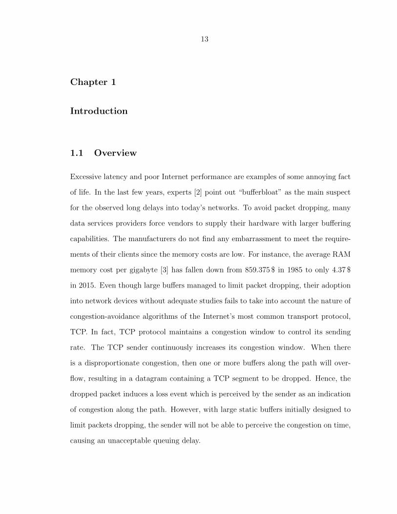
1.1 Overview
Excessive latency and poor Internet performance are examples of some annoying fact
of life. In the last few years, experts [2] point out “bufferbloat” as the main suspect
for the observed long delays into today’s networks. To avoid packet dropping, many
data services providers force vendors to supply their hardware with larger buffering
capabilities. The manufacturers do not find any embarrassment to meet the require-
ments of their clients since the memory costs are low. For instance, the average RAM
memory cost per gigabyte [3] has fallen down from 859.375 $ in 1985 to only 4.37 $
in 2015. Even though large buffers managed to limit packet dropping, their adoption
into network devices without adequate studies fails to take into account the nature of
congestion-avoidance algorithms of the Internet’s most common transport protocol,
TCP. In fact, TCP protocol maintains a congestion window to control its sending
rate. The TCP sender continuously increases its congestion window. When there
is a disproportionate congestion, then one or more buffers along the path will over-
flow, resulting in a datagram containing a TCP segment to be dropped. Hence, the
dropped packet induces a loss event which is perceived by the sender as an indication
of congestion along the path. However, with large static buffers initially designed to
limit packets dropping, the sender will not be able to perceive the congestion on time,
causing an unacceptable queuing delay.
14
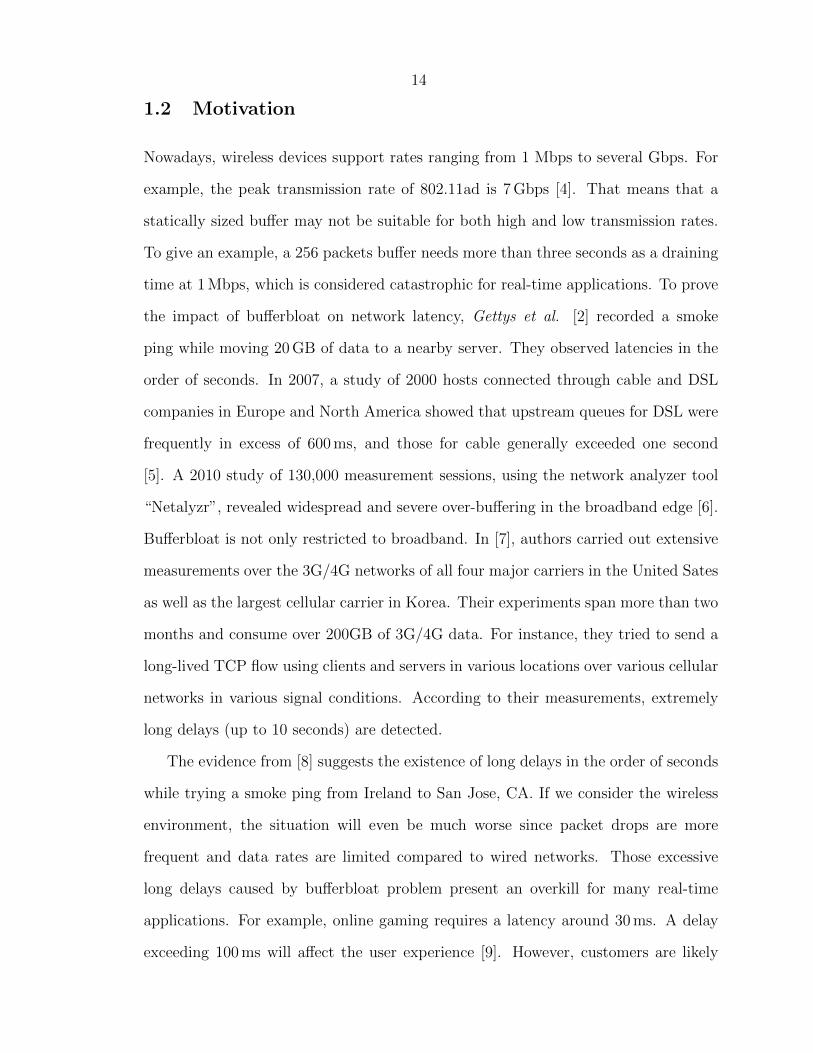
1.2 Motivation
Nowadays, wireless devices support rates ranging from 1 Mbps to several Gbps. For
example, the peak transmission rate of 802.11ad is 7 Gbps [4]. That means that a
statically sized buffer may not be suitable for both high and low transmission rates.
To give an example, a 256 packets buffer needs more than three seconds as a draining
time at 1 Mbps, which is considered catastrophic for real-time applications. To prove
the impact of bufferbloat on network latency, Gettys et al. [2] recorded a smoke
ping while moving 20 GB of data to a nearby server. They observed latencies in the
order of seconds. In 2007, a study of 2000 hosts connected through cable and DSL
companies in Europe and North America showed that upstream queues for DSL were
frequently in excess of 600 ms, and those for cable generally exceeded one second
[5]. A 2010 study of 130,000 measurement sessions, using the network analyzer tool
“Netalyzr”, revealed widespread and severe over-buffering in the broadband edge [6].
Bufferbloat is not only restricted to broadband. In [7], authors carried out extensive
measurements over the 3G/4G networks of all four major carriers in the United Sates
as well as the largest cellular carrier in Korea. Their experiments span more than two
months and consume over 200GB of 3G/4G data. For instance, they tried to send a
long-lived TCP flow using clients and servers in various locations over various cellular
networks in various signal conditions. According to their measurements, extremely
long delays (up to 10 seconds) are detected.
The evidence from [8] suggests the existence of long delays in the order of seconds
while trying a smoke ping from Ireland to San Jose, CA. If we consider the wireless
environment, the situation will even be much worse since packet drops are more
frequent and data rates are limited compared to wired networks. Those excessive
long delays caused by bufferbloat problem present an overkill for many real-time
applications. For example, online gaming requires a latency around 30 ms. A delay
exceeding 100 ms will affect the user experience [9]. However, customers are likely

15
to abandon a game when they experience a network delay of 500 milliseconds. VoIP
cannot tolerate delays larger than 150 ms to ensure the intended level of QoS. Amazon
observed that they lose 1 % of sales for each additional 100 ms of latency [10], which
translates to more than one billion dollars loss.
To further confirm previous findings, we conducted a simple experiment. We send
a fully backlogged data flow between an access point and a station for 100 s. Both
nodes are configured with static buffers that can accommodate up to 400 packets. We
track both the Round Trip Time (RTT) for the DATA/ACK exchange in the MAC
layer and the queuing delay at the sender node. We found that the RTT is around
524µs. Indeed, the RTT in the 802.11’s link-layer acknowledgment scheme is mostly
deterministic, composed of the Waveform TX time (depends on the packets length
and TX rate), propagation time (depends on the nodes separation, negligible relative
to the other components), SIFS duration (fixed at 16µs) and RX start delay (fixed
at ∼25 µs). Regarding the buffering delay, the average queuing latency is 268 ms and
the maximum is 602 ms. Using the best possible achievable throughput of ∼30 Mbps,
it would take logically 160 ms to drain the queue. This experiment confirms that the
queuing delay is really behind the long latency that we observe in today’s networks.
1.3 Thesis Outline
In this work, we aim to control the latency in wireless networks without incurring
significant costs in term of other important network performance metrics. The rest
of this thesis is organized as follows. The next chapter examines the state of the
art solutions for bufferbloat, their strengths, and their limitations. In addition, we
highlight the challenges that we face in designing efficient solutions for this problem.
In chapter 3, we address the issue of bufferbloat in wireless full-duplex systems. We
propose using the Wireless Queue Management (WQM) mechanism [11] to manage
the buffers in full-duplex nodes. WQM dynamically adjusts the buffer size according

16
to the queue draining time and its current size. To the best of our knowledge, this work
is the first attempt to address the buffer management issues in wireless full-duplex
systems. We demonstrate through simulation that WQM has succeeded to decrease
latency by two orders of magnitude while achieving similar throughput compared to
Drop Tail mechanism. WQM tries to maintain the buffer size around an optimal
value. However, it requires complicated initial parameters setting based on the Wi-
Fi standard used. Also, it is more biased towards latency and does not account
for throughput variation. To overcome those limitations, in chapter 4, we present a
reinforcement learning based buffer management scheme for wireless networks, called
“LearnQueue”. LearnQueue has the same basic concept of WQM. In fact, it tunes
the buffer size dynamically to maintain the desired Quality of Service (QoS). The
congestion detection relies on a reward function that accounts for the balance between
latency trends and dropping rates in the queue. Our testbed results demonstrate that
LearnQueue can control the latency around a reference value using the previously
learned experience and the immediate feedback from the network without impacting
the link utilization. Furthermore, LearnQueue does not incur extra overhead and
adapts rapidly under various network scenarios. Conclusions are finally drawn in
chapter 5.
17
Chapter 2
Fighting Bufferbloat in Wireless Networks
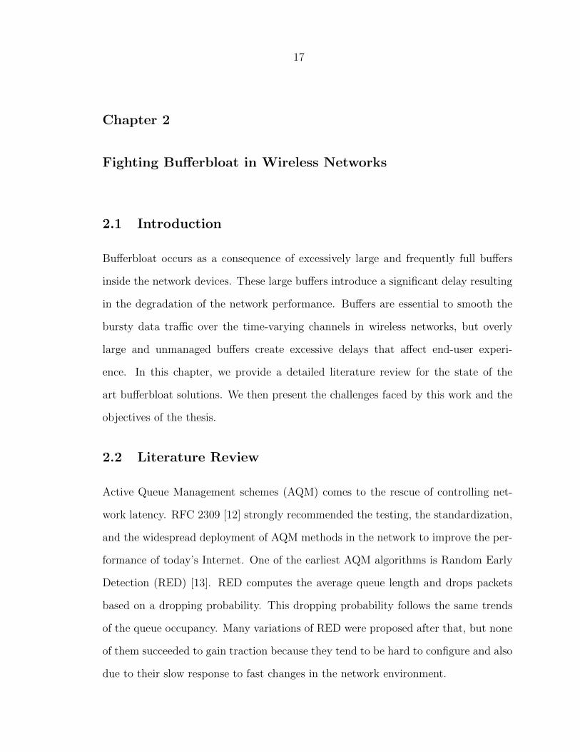
2.1 Introduction
Bufferbloat occurs as a consequence of excessively large and frequently full buffers
inside the network devices. These large buffers introduce a significant delay resulting
in the degradation of the network performance. Buffers are essential to smooth the
bursty data traffic over the time-varying channels in wireless networks, but overly
large and unmanaged buffers create excessive delays that affect end-user experi-
ence. In this chapter, we provide a detailed literature review for the state of the
art bufferbloat solutions. We then present the challenges faced by this work and the
objectives of the thesis.
2.2 Literature Review
Active Queue Management schemes (AQM) comes to the rescue of controlling net-
work latency. RFC 2309 [12] strongly recommended the testing, the standardization,
and the widespread deployment of AQM methods in the network to improve the per-
formance of today’s Internet. One of the earliest AQM algorithms is Random Early
Detection (RED) [13]. RED computes the average queue length and drops packets
based on a dropping probability. This dropping probability follows the same trends
of the queue occupancy. Many variations of RED were proposed after that, but none
of them succeeded to gain traction because they tend to be hard to configure and also
due to their slow response to fast changes in the network environment.
18
In 2012, an AQM scheme called CoDel [14] was proposed. CoDel monitors the
packet sojourn time in the queue. For a given interval, the algorithm finds the lowest
queuing delay experienced by all packets. If the lowest packet sojourn time over a
predefined interval exceeds the target, the packet is dropped, and the interval will
be shortened. Alternatively, if the lowest packet sojourn time for that interval is
still in the acceptable range, the packet is forwarded, and the interval is reset to 100
milliseconds (initial default value). This algorithm was essentially designed to detect
bad queues, which are defined as the queues that last longer than one RTT resulting
in a constantly high buffering latency. CoDel is a self-configurable algorithm and has
shown good performance over traditional AQM solutions [15]. However, it requires
per-packet timestamps and drops packets after spending some time in the queue,
wasting all resources used for maintaining and processing those packets.
Later, PIE (Proportional Integral controller Enhanced) [8] was introduced. Similar
to CoDel, PIE randomly drops a packet when experiencing congestion. The drop
probability is computed based on the deviation of the queuing delay from a predefined
target and the direction where the delay is moving. PIE does not require per-packet
extra processing. Moreover, it is highly responsive to sudden changes in the network
conditions. However, PIE considers only latency trends without looking at how much
packets are dropped in the queue.
Neither CoDel nor PIE were originally designed for operation in wireless networks.
In 2014, authors of [11] proposed Wireless Queue Management (WQM), a dynamic
buffer sizing scheme that addressed the unique challenges of wireless networks. WQM
adjusts the buffer size according to the queue draining rate.
In a systemic evaluation of the bufferbloat effect, Cardozo et al. [16] suggested
that bufferbloat might be resulting from different layers of buffering. Considering
the microscopic view of the buffer architecture of typical network devices, they drew
attention to the impact of varying the size of various buffers in the network transmit

19
stack, especially ring buffer, which is a circular buffer associated with the network
card in Unix-based architecture. Through a typical home network scenario with
a single bottleneck, the authors demonstrated that the variation of the ring buffer
leads to high RTTs. Their speculative claim aims to turn the efforts of mitigating
the bufferbloat impact to focus more on ring buffers sizing instead the conventional
transmit buffers. Unfortunately, a serious weakness within this argument is that the
ring buffers lack flexibility, which makes their access and control a complicated task.
Besides, the results of this research cannot be taken for granted since the experiments
are conducted in a very limited scope of scenarios.
In Linux kernel 3.3, a new functionality known as Byte Queue Limits (BQL) has
been introduced [17]. BQL is a self-regulating algorithm that intends to estimate
the limits of packets data which can be put in the transmission queue of a network
interface. Using BQL, we can control and reduce the number of packets sent to the
ring buffer, shifting the queuing to upper layers. The use of BQL combined with
queue disciplines like CoDel can drastically reduce the latency [16].
We should notice that AQM based solutions are not the only proposals aiming at
fighting the bufferbloat phenomenon. In the transport layer, some proposed methods
keep the network core unaltered. The adaptation of such solutions is restricted to
the end hosts. Those solutions come into sight with the engineering of end-to-end
flows and congestion control alternatives to best-effort TCP. Congestion and flow
control may have different objectives than AQM techniques, such as controlling the
streaming rate over TCP connections as done by YouTube or Netflix, or aggressively
protecting user QoE as done by Skype over UDP. In their seminal paper of 2012, the
authors proposed Dynamic Receive Window Adjustment (DRWA) [7], a delay-based
congestion control algorithm that modifies the existing receive window adjustment
algorithm of TCP to control the sending rate indirectly. DRWA increases the receive
window when the current RTT is close to the minimum RTT observed and decreases

20
it when RTT becomes larger due to the queuing delay. With proper parameters
tuning, DRWA succeeded to keep the queue size at the bottleneck link small enough
so that throughput and delay experienced by a TCP flow are both optimized. The
results show that DRWA reduces the RTT by 25 % to 49 % while achieving similar
throughput. Congestion control methods have the advantage to be lightweight and
easy to deploy, especially with devices with limited resources such as cellular phones.
2.3 Challenges
In this section, we highlight the challenges faced by this work. AQM are the most
common solutions to overcome the problem of bufferbloat. The design of the AQM
schemes should follow certain specific criteria:
� Low latency control: We control the queuing latency in wireless devices by
directly controlling the queue size. In this way, we avoid unnecessary dropping
of packets in order to get the targeted delay. Hence, the low latency can be
achieved without affecting high link utilization. In fact, an early congestion
signal could lead TCP to back off and reduce its rate. Therefore, this rate
reduction could result in link under-utilization.
� Meeting applications requirements: Some applications are sensitive to de-
lays and jitter such as video gaming while others are biased towards dropping
(e.g., video streaming). Any proposed scheme should introduce tuning param-
eters to meet the applications specific requirements in terms of latency and
packet loss.
� The specificities of wireless environment: The wireless environment is
very challenging. It usually causes random bit errors to occur in short bursts,
thus, leading to a higher probability of multiple random packet losses. In TCP
21
protocol, such packet losses are wrongly inferred to be the result of network con-
gestion and would mistakenly trigger the TCP sender to reduce its sending rate
unnecessarily. In addition, a packet may be transmitted multiple times before it
is successfully received, resulting in inter-service delays variation. Hence, more
than one factor influences the congestion signal in wireless links. The designed
scheme should continuously learn from the environment with a critic to build
useful experience and try to predict the long-term desirability of each state.
� Responsiveness and stability: The system should guarantee agility to sud-
den changes in the network. Besides, it should ensure system stability for various
streams types, network topologies, and data rates. This requirement is crucial
for wireless systems where links rates change dynamically, and the spectrum is
a shared resource between a set of neighboring nodes.
� Wireless full-duplex: In full-duplex WLANs, a station can receive data from
the AP while it is transmitting its own data. This impacts the queuing delay
experienced by individual frames, thus, affecting the buffering requirements at
the station or the access point. As a first step, the impact of those changes need
to be quantified and, then, the existing buffer sizing work should be adapted
for operation in wireless full-duplex.
� Multi-hop challenge: In multi-hop networks, instead of considering the per-
formance of individual components, we need to improve the performance of the
entire system. Due to the shared nature of wireless spectrum, a flow will not
only compete for transmission opportunities with other flows from the same
source but also contends with other flows from different nodes along the hops
to the destination. This adds to the challenges mentioned above. A flow may
traverse more than one hop to reach its final destination (Ad-Hoc mode). As a
result, packets may spend time at more than one queue and experience higher
22
level of channel contention, especially with increased visibility between different
nodes. The queuing delay, in this case, will span multiple nodes and may reach
higher values than expected.
2.4 Objectives
Buffers are introduced in networks to absorb transient bursts. The latency a packet
experiences in a network is made up of transmission delay (time it takes to push
the packet’s bits into the link), processing delay (time routers take to process the
packet header), propagation delay (time for a signal to reach its destination) and
queuing delay (time the packet spends in the routing queues). In a multi-hop sce-
nario, packets cannot reach their final destination faster than the time it takes to
send a packet at the bottleneck rate. Figure 2.1 shows the relationship between delay
and throughput considering the buffering issues. Large buffers result in long queuing
delays, while very small buffers may lead to network under-utilization due to higher
packet loss rate. A network with no buffers has no room for packets ready for trans-
mission. Therefore, extra packets will be dropped, causing an increasing loss rate and
decreasing throughput. This research was carried out in order to mitigate the large
end-to-end latency and jitter as well as the throughput degradation resulting from
oversized queues. Our contributions to address the above-mentioned challenges are
as follows:
� The problem of bufferbloat in wireless networks has not been studied system-
atically. We investigate this issue and its impact on wireless links performance.
� We proposed simple and easily deployable solutions that are experimentally
proven to be effective and highly responsive.
� We conducted extensive measurements in a range of 802.11 wireless networks
using various traffic types and characterized the bufferbloat problem in different

23
Figure 2.1: Relationship between delay and throughput.
network conditions.
� We investigate the problem of buffer management in wireless full-duplex sys-
tems. Our results suggest that bufferbloat is an important issue to consider in
developing the next-generation wireless technologies.
� To the best of our knowledge, we are the first to employ artificial intelligence
and reinforcement learning techniques in solving bufferbloated networks issues.
� Our solutions are protocol-independent, imply little or no cost and does not
incur extra overhead in the network.
� We introduce scaling weights to control the bias of the model towards latency
or packet loss rate depending on specific applications requirements.
24
Chapter 3
Buffer Management in Wireless Full-Duplex Systems
3.1 Introduction
The long-held assumption that wireless devices should operate in half-duplex mode
persisted for many years before the appearance of the full-duplex systems. In fact,
traditionally, a radio cannot receive and transmit simultaneously on a single channel
because the receive antenna of the wireless device will hear its own transmissions
which are hundreds to thousands of times stronger than the transmissions coming
from other nodes. Full-duplex systems [18, 19] have succeeded in challenging this
assumption by using cancellation techniques to cancel self-interference and eliminating
the noise created by the transmit signal.
Beyond increasing throughput, full-duplex systems have shown great potential to
solve some critical problems with existing wireless networks such as hidden terminals,
loss of throughput due to congestion, and large end-to-end delays [18]. In fact, the
idea of receiving and forwarding simultaneously can reduce the large end-to-end delays
in multi-hop networks since a full-duplex node can simultaneously start forwarding a
packet to the next hop while receiving it. However, with today’s bloated networks,
full-duplex relaying is not sufficient to solve the problem of high latency. For instance,
wired networks operate in full-duplex mode and still suffer from unacceptable delays.
If we take into consideration the fact that wireless spectrum is a shared resource
between a set of neighboring nodes even in full-duplex mode in which a node can
receive or transmit to many others, the situation will be worse. Existing wireless

25
full-duplex designs should give real answers to related engineering challenges before
finding their own way to the industry and large scale deployments.
To address the issue of bufferbloat in wireless full-duplex systems, we propose
using the “Wireless Queue Management” (WQM) mechanism to manage the buffers
in the full-duplex nodes. To the best of our knowledge, this is the first work that
shed lights on the queuing disciplines in wireless full-duplex systems. Our evaluation
shows that WQM managed to decrease latency by two orders of magnitude. With an
increasing number of nodes, it achieved better throughput than Drop Tail.
3.2 Wireless Full-Duplex
Nowadays, wireless devices generally operate in half-duplex mode which means they
can either transmit or receive on a single channel, but not do both at the same time.
Recent research proved that full-duplex is feasible with the use of interference cancel-
lation techniques. Choi et al. [18] succeeded to achieve a single channel full-duplex
wireless communication by implementing a full-duplex IEEE 802.11.4 testbed using
two USRP v1 [20] equipped with two 2.4 GHz radio RFX 2400 daughterboards. In
their design, they introduced a novel self-interference cancellation scheme called “An-
tenna Cancellation”. The insight behind antenna cancellation is that transmissions
from two antennas could be added destructively where a separate receive antenna is
placed in a specific location. For the signals to be added destructively and cancel
each other for a wavelength λ, we should place the transmitters at distances d and
d+ λ2
away from the receive antenna. Antenna cancellation provided about 30 dB of
self-interference cancellation. Combined with analog cancellation based on QHx220
noise canceler chip and digital cancellation, it succeeded to cancel about 60 dB of
interference. Overall, single channel full-duplexing gives a gain of 84 % in throughput
without a significant loss in network reliability. However, this design presents many
limitations. First of all, the prototype uses 7 inches of spacing between antennas which
26
makes it unsuitable for today’s small wireless cards. In addition, it supports neither
wide bandwidths like the 20 MHz 802.11 Wi-Fi signals nor high transmit powers.
Moreover, antenna cancellation is very sensitive to antennas placement mismatch.
To overcome these limitations, Jain et al. [19] proposed a full-duplex radio de-
sign based on a balanced/unbalanced (Balun) transformer. The mechanism known
as “Balun Cancellation” exploits signal inversion using a balun circuit in an adap-
tive manner to match the self-interference signal. This design, unlike the antenna
cancellation, eliminates the bandwidth constraint and supports high transmit pow-
ers. Balun cancellation combined with digital cancellation can achieve up to 73 dB
of cancellation for a 10 MHz OFDM signal. While it solves many problems related
to full-duplex, this cancellation technique is very sensitive to delays and needs very
sophisticated electronic components. Further, TX and RX antennas are separated by
20 cm which represents a major engineering limitation especially for mobile devices
like tablets and mobile phones.
In 2012, a group of researchers from Rice University [21] implemented a practi-
cal 20 MHz IEEE 802.11 multi-antenna full-duplex system using WARP boards [22].
Their design almost achieves the intended doubling of throughput. Despite the fact
that this prototype succeeded to extend the practical range of full-duplex Wi-Fi, it is
based on a non-real time design and uses the CM-MMCX clock module [23] for the
synchronization of the wireless devices reference clocks, which may break down the
concept of wireless communication as a whole. In the same year, Hong et al. [24]
introduced a transparent spectrum slicing scheme called “Picasso” which allows si-
multaneous transmission and reception on separate and arbitrary spectrum fragments
using a single antenna. Picasso solves the problem of leaking of interference into the
adjacent spectrum, especially in Wi-Fi OFDM signals. Later, other implementations
of full-duplex systems appeared such as the implementation of the full-duplex 802.11ac
radio using a single antenna for both transmit and receive [25]. This achievement was
27
made possible thanks to the use of an analog cancellation board and a circulator.
With more sophisticated digital and analog cancellation techniques, the prototype
reduces self-interference by 110 dB and achieves a median throughput gain of 1.87x.
The research about full-duplex did not stop at this point. Bharadia and Katti [26]
demonstrated that full-duplex could be combined with MIMO systems putting an
end to comparisons between the performance of MIMO half-duplex and full-duplex
systems. Conceiving a MIMO full-duplex design wasn’t a simple task because a
single antenna will not only suffer from the ordinary self-interference but also from
a very strong cross-talk coming from neighboring antennas in the TX chain. The
replication of SISO full-duplex is considered as ineffective due to several complexity
and scalability limitations. In order to reduce complexity, the design exploits the
fact that neighboring MIMO antennas share a similar radio environment. Hence, the
solution was based on creating a cascaded filter structure composed of M cancellation
circuits for M-antennas MIMO system that leaves a negligible 1 dB of the overall
self-interference. Moreover, digital cancellation was used to cancel any residual self-
interference. The experimental setup of 3 x 3 Wi-Fi MIMO ensures a 95 % gain in
throughput compared to half-duplex.
3.3 Approach
Typically, wireless devices have both receive and transmit buffers. However, receive
buffers usually do not cause bufferbloat since the actual wireless devices possess good
processing capabilities. More precisely, wireless nodes process incoming packets and
forward those packets to the transmit queue if this node is not their final destination
or to the backbone network in the other case. Thus, we should focus on transmit
buffers which are really beyond the increase in the network latency. We believe that
we can reuse the same approach as half-duplex adaptive buffer sizing in the full-duplex
domain with small changes. Adaptive buffer sizing can also be used to improve the

28
energy efficiency of radio design. However, we must consider several challenges in
designing a dynamic buffer sizing method that goes hand in hand with wireless full-
duplex. The most interesting possible benefits of full-duplex occur above the physical
layer. Multi-hop networks suffer from long end-to-end delays, which are harmful
to delay-sensitive protocols like TCP. Further, multi-hop networks experience less
throughput scaling compared to single-hop networks due to the interference between
forwarding hops. Instead of the traditional store-and-forward architecture, full-duplex
nodes can simultaneously start to transmit a packet, while receiving it.
Our primary goal is to deploy an AQM technique on a full-duplex system and ana-
lyze the performance. We already know the performance of many buffer management
techniques on wireless half-duplex systems even though the majority of them were
designed for wired networks. Nevertheless, there is a lack in the literature about the
suitable method to manage the buffer of a full-duplex node or what is the impact of
such techniques on networks metrics like latency and throughput. For this purpose,
we need to setup a wireless full-duplex testbed and modify the buffer module in order
to stimulate the wanted adaptive buffer management behavior. The AQM techniques
previously discussed in the chapter 2 are not initially designed for wireless networks.
They may not be capable of supporting different challenges related to the wireless
medium like changing transmission rates, frame aggregation, link scheduling, etc.
Showail et al. [11] proposed “Wireless Queue Management” (WQM), a queue man-
agement scheme for wireless networks. WQM is an adaptive buffer sizing algorithm
that estimates periodically the buffer draining time using the current transmission
rate, backlog queue and the number of neighboring nodes. WQM algorithm varies
the buffer size depending on buffer draining time. An alarm is raised when exceeding
a predefined value, and the buffer size will be reduced as a result. In comparison to
CoDel and PIE, WQM demonstrates an excellent performance in an ordinary IEEE
802.11n half-duplex testbed. The novelty of WQM lies in the fact that it is designed

29
to address the unique challenges of buffer sizing in wireless networks [27]. In reality,
WQM is the first queue management technique that is aggregation-aware, that is to
say, it accounts for frame aggregation when selecting the buffer size in wireless net-
works. Second, the link rate in wireless networks changes dynamically in response
to variations in network conditions. The capacity of the network controls the BDP
(Bandwith-Delay Product) which reflects the amount of buffering needed in the net-
work. To address this issue, WQM is the only scheme in the literature that is tightly
coupled with the rate control algorithm to quickly respond to changes in the envi-
ronment. Last but not least, WQM accounts for the number of active users when
selecting the optimal buffer size. This number affects the packet service rate due to
MAC random scheduling in wireless networks. All those advantages motivated us to
implement WQM in the top of a wireless full-duplex testbed with minor changes.
3.4 Implementation
We based our work on a simulation of full-duplex communication in a multi-hop
context using the discrete-event network simulator NS-3 [28]. This simulation deploys
the Relay Full-Duplex MAC protocol [29] by extending the Wi-Fi module [1] of NS-
3.20. Relay Full-Duplex MAC (RFD-MAC) is a media access control protocol which
is designed for relay full-duplexing. Multi-hop networks can handle bidirectional full-
duplexing as well as relay full-duplexing. Relay full-duplex situation occurs when
node 2 receives a frame from node 1 while forwarding a frame to node 3 as shown
in figure 3.1. To maximize the full-duplex capability, RFD-MAC should properly
choose a secondary transmission node. For example, node 2 has two candidates for
a secondary transmission node: nodes 1 and 3. If the MAC protocol selects a node
that does not have a frame, then, relay full-duplexing does not occur.
Also, RFD-MAC takes into account the possible collision between a primary trans-
mission and a secondary transmission. A collision occurs at receiver node when a

30
Figure 3.1: Bidirectional full-duplexing vs. Relay full-duplexing.
primary transmission node is placed within the transmission range of a secondary
transmission node and vice versa. Every node builds its own surrounding node table
and exploits this table to choose a secondary transmission node in such a way that
avoids a collision between primary and secondary transmissions. The algorithm of
selecting a secondary node is based on a priority set. Whenever a node completes
the transmission of the frame before receiving is done, RFD-MAC uses a busytone
until the reception is complete. Then, the primary and secondary transmission nodes
exchange ACK frames to finalize the full-duplex transmission session as shown in
figure 3.2. This scheme does not completely eliminate collision because the receiver
is susceptible to collisions until it finishes receiving the packet header.
Figure 3.2: RFD-MAC time sequence.
NS-3 was built to improve the realism of the models and architected similar to
Linux computers with the intention of being used on testbeds and real devices and

31
applications [30]. “WifiNetDevice” models are the objects that we deploy to create
802.11-based infrastructure and Ad-Hoc networks. In the Wi-Fi module of NS-3, the
“WifiNetDevice” internal queues have different architecture than the traditional ones
used elsewhere. Figure 3.3 shows the module architecture. The insight beyond our
work is to handle the transmit packet queue “m queue” via modifying “Enqueue”
function belonging to “WifiMacQueue” class. The source code of the simulation is
available with executable scripts at [31].
Figure 3.3: “WifiNetDevice” module architecture [1].
We would like to note that our current implementation presents some minor differ-
ences with the original WQM implementation. First, our testbed deploys an Ad-Hoc
Wi-Fi network based on IEEE 802.11a standard [32] in which the transmission range
can vary between 6 Mbps and 54 Mbps. All devices are configured with Adaptive
Auto Rate Fallback (AARF) rate control algorithm [33] instead of Minstrel. AARF
tries to increase the transmission rate after a set number of successful transmissions
32
at the current rate. To ensure the stability of the channel, AARF increases the suc-
cess threshold it needs before it tries to use a higher rate by remembering the number
of failed probes. In case of two consecutive packet losses, it lowers the transmission
rate one step and resets the success threshold to ten. In its original version, WQM
is synchronized with Minstrel which is tuned every 100 ms. This is not the case for
our current setup since AARF is based on packet transfer success or failure. Thus,
we choose simply to run the algorithm periodically on every incoming packet to the
transmit queue. Second, the simulation of full-duplex communication [28] uses a high
MAC layer that is not QoS-enabled and hence it does not support frame aggregation.
So, we modify the WQM algorithm to deal with disabled frame aggregation.
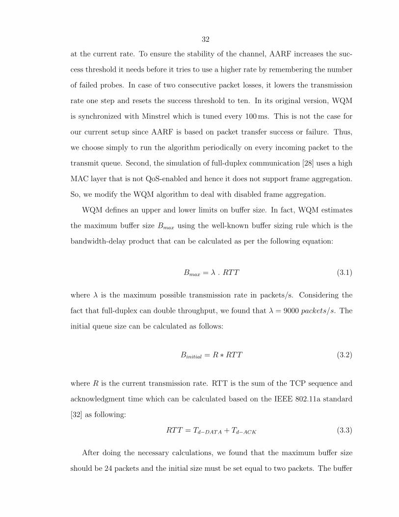
WQM defines an upper and lower limits on buffer size. In fact, WQM estimates
the maximum buffer size Bmax using the well-known buffer sizing rule which is the
bandwidth-delay product that can be calculated as per the following equation:
Bmax = λ . RTT (3.1)
where λ is the maximum possible transmission rate in packets/s. Considering the
fact that full-duplex can double throughput, we found that λ = 9000 packets/s. The
initial queue size can be calculated as follows:
Binitial = R ∗RTT (3.2)
where R is the current transmission rate. RTT is the sum of the TCP sequence and
acknowledgment time which can be calculated based on the IEEE 802.11a standard
[32] as following:
RTT = Td−DATA + Td−ACK (3.3)
After doing the necessary calculations, we found that the maximum buffer size
should be 24 packets and the initial size must be set equal to two packets. The buffer
33
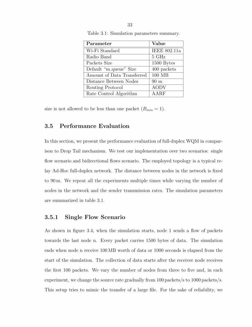
Table 3.1: Simulation parameters summary.
Parameter Value
Wi-Fi Standard IEEE 802.11aRadio Band 5 GHzPackets Size 1500 BytesDefault “m queue” Size 400 packetsAmount of Data Transferred 100 MBDistance Between Nodes 90 mRouting Protocol AODVRate Control Algorithm AARF
size is not allowed to be less than one packet (Bmin = 1).
3.5 Performance Evaluation
In this section, we present the performance evaluation of full-duplex WQM in compar-
ison to Drop Tail mechanism. We test our implementation over two scenarios: single
flow scenario and bidirectional flows scenario. The employed topology is a typical re-
lay Ad-Hoc full-duplex network. The distance between nodes in the network is fixed
to 90 m. We repeat all the experiments multiple times while varying the number of
nodes in the network and the sender transmission rates. The simulation parameters
are summarized in table 3.1.
3.5.1 Single Flow Scenario
As shown in figure 3.4, when the simulation starts, node 1 sends a flow of packets
towards the last node n. Every packet carries 1500 bytes of data. The simulation
ends when node n receive 100 MB worth of data or 1000 seconds is elapsed from the
start of the simulation. The collection of data starts after the receiver node receives
the first 100 packets. We vary the number of nodes from three to five and, in each
experiment, we change the source rate gradually from 100 packets/s to 1000 packets/s.
This setup tries to mimic the transfer of a large file. For the sake of reliability, we

34
have done at least two trials for each experiment, and the results are averaged. The
corresponding results are shown in figures 3.5, 3.6 and 3.7. We draw the attention of
the reader that we used the logarithmic scale for the y-axis in the latency figures for
more clarity.
Figure 3.4: Topology of single flow scenario.
As expected, WQM outperforms Drop Tail in terms of latency reduction. When
the network is bloated, WQM reduces the latency by an average of 109x for the three
nodes case, 208x for the four nodes case and 49x for the five nodes case. In com-
parison to Drop Tail, this reduction corresponds to 99 % of total network latency.
For example, in the four nodes setup and using a sender rate of 800 packets/s, WQM
reduces the end-to-end delay from 4094.51 ms in the default case to only 18.91 ms,
which represents two orders of magnitude reduction. In addition, in the three ex-
periments, we clearly see a latency in order of seconds for the default buffering case.
When the source rate reaches more than 300 packets/s, the network latency varies
around one second for the three nodes setup, around four seconds for the four nodes
setup and varies between 1.07 s and 1.48 s for the five nodes setup. On the contrary,
WQM maintains a latency less than 10.27 ms for the three nodes topology, less than
20.69 ms for the four nodes topology and less than 29.32 ms for the five nodes topol-
ogy. It is obvious from these figures that controlling the size of buffers and adapting
them to fast changes in the network results in significant queuing delay reduction.
We would like to note that WQM causes only 9 % average drop in goodput for the
three nodes case. However, when we increase the number of hops, WQM improves
the network goodput. In average, it achieves about 7.7 % and 25 % of increase in
35
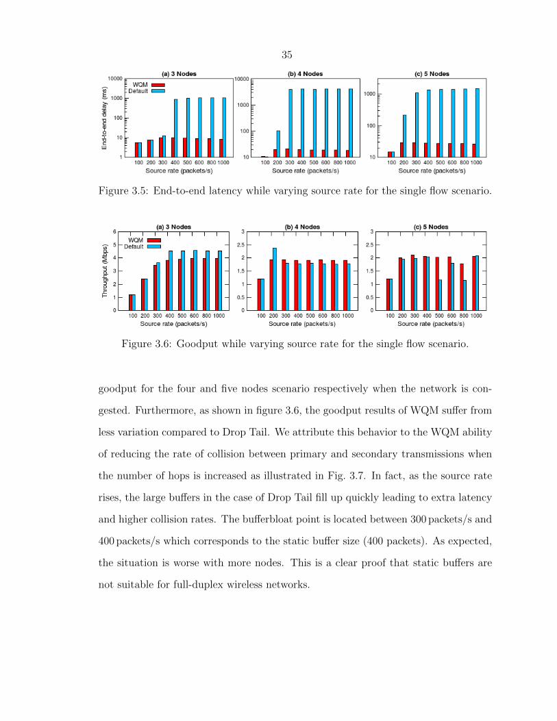
Figure 3.5: End-to-end latency while varying source rate for the single flow scenario.
Figure 3.6: Goodput while varying source rate for the single flow scenario.
goodput for the four and five nodes scenario respectively when the network is con-
gested. Furthermore, as shown in figure 3.6, the goodput results of WQM suffer from
less variation compared to Drop Tail. We attribute this behavior to the WQM ability
of reducing the rate of collision between primary and secondary transmissions when
the number of hops is increased as illustrated in Fig. 3.7. In fact, as the source rate
rises, the large buffers in the case of Drop Tail fill up quickly leading to extra latency
and higher collision rates. The bufferbloat point is located between 300 packets/s and
400 packets/s which corresponds to the static buffer size (400 packets). As expected,
the situation is worse with more nodes. This is a clear proof that static buffers are
not suitable for full-duplex wireless networks.
36
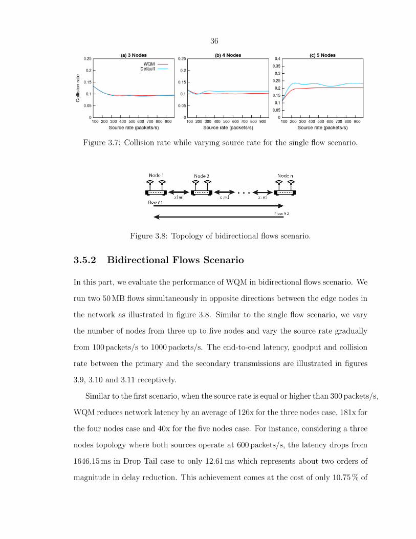
Figure 3.7: Collision rate while varying source rate for the single flow scenario.
Figure 3.8: Topology of bidirectional flows scenario.
3.5.2 Bidirectional Flows Scenario
In this part, we evaluate the performance of WQM in bidirectional flows scenario. We
run two 50 MB flows simultaneously in opposite directions between the edge nodes in
the network as illustrated in figure 3.8. Similar to the single flow scenario, we vary
the number of nodes from three up to five nodes and vary the source rate gradually
from 100 packets/s to 1000 packets/s. The end-to-end latency, goodput and collision
rate between the primary and the secondary transmissions are illustrated in figures
3.9, 3.10 and 3.11 receptively.
Similar to the first scenario, when the source rate is equal or higher than 300 packets/s,
WQM reduces network latency by an average of 126x for the three nodes case, 181x for
the four nodes case and 40x for the five nodes case. For instance, considering a three
nodes topology where both sources operate at 600 packets/s, the latency drops from
1646.15 ms in Drop Tail case to only 12.61 ms which represents about two orders of
magnitude in delay reduction. This achievement comes at the cost of only 10.75 % of

37
Figure 3.9: End-to-end latency while varying source rate for the bidirectional flowsscenario.
Figure 3.10: Goodput while varying source rate for the bidirectional flows scenario.
reduction in goodput. For the three nodes setup, in limited cases, we see some impor-
tant goodput drops, exactly at the measurement points 800 and 1000 packets/s, that
reach 50 %. However, sacrificing 50 % of throughput to get 99 % of latency reduction
still a good deal for some delay-sensitive applications.
Further, as long as we increase the number of nodes, the same effect as the first
scenario occurs: the goodput increases as well. In the five nodes setup, the average
increase in goodput is about 24 %. Unlike the single flow scenario, in the four nodes
topology, Drop Tail still have slightly better goodput in several cases even though
WQM succeed to reduce the collision rate as shown in figure 3.11. We investigate
this issue and finally, we find that WQM have inferior full-duplex ratio in this case
as shown in figure 3.12. This reduction varies between 2.87 % and 8.81 % in compar-
ison to Drop Tail and may limit the ability of WQM to increase goodput by taking
advantage of the improvement in the collision rate. Despite this limitation, WQM
38
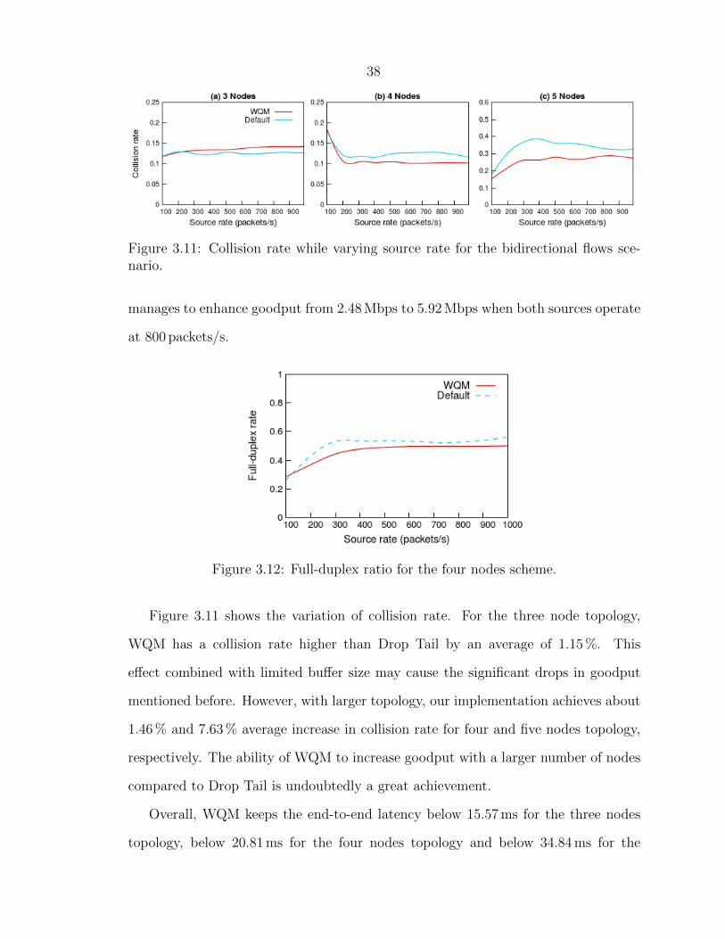
Figure 3.11: Collision rate while varying source rate for the bidirectional flows sce-nario.
manages to enhance goodput from 2.48 Mbps to 5.92 Mbps when both sources operate
at 800 packets/s.
Figure 3.12: Full-duplex ratio for the four nodes scheme.
Figure 3.11 shows the variation of collision rate. For the three node topology,
WQM has a collision rate higher than Drop Tail by an average of 1.15 %. This
effect combined with limited buffer size may cause the significant drops in goodput
mentioned before. However, with larger topology, our implementation achieves about
1.46 % and 7.63 % average increase in collision rate for four and five nodes topology,
respectively. The ability of WQM to increase goodput with a larger number of nodes
compared to Drop Tail is undoubtedly a great achievement.
Overall, WQM keeps the end-to-end latency below 15.57 ms for the three nodes
topology, below 20.81 ms for the four nodes topology and below 34.84 ms for the
39
five nodes topology, which is an acceptable delay for real-time applications like VoIP,
online gaming, video streaming, etc. As mentioned earlier, WQM manages the buffers
in an effective manner and prevents the large buffers buildup at the bottleneck links.
3.6 Conclusion
This chapter tackles the problem of buffer management in wireless full-duplex systems
and analyses the gains in terms of latency of implementing AQM on the top of such
systems. We proved through simulation using NS-3 over several scenarios that WQM,
an adaptive buffer sizing algorithm, can decrease latency in a relay full-duplex testbed
by two orders of magnitude. Besides, we provided some essential background material
about the evolution of wireless full-duplex systems. We believe that this work opens
a new research direction by evaluating the interaction between buffer management
techniques and full-duplex design.
40
Chapter 4
Latency Control in Wireless Networks Employing
Reinforcement Learning
4.1 Introduction
This chapter is devoted to introduce a novel design called “LearnQueue” based on
reinforcement learning that can effectively control the latency in wireless networks.
LearnQueue accounts for both delay and dropping to avoid the extra packet losses
introduced by most traditional AQM techniques. The rest of this chapter is organized
as follows. The next section describes the LearnQueue design. The third section
provides our testbed implementation details. After that, we present and analyze the
extracted results.
4.2 LearnQueue Scheme Design
In this section, we describe the design of LearnQueue, its parameters settings and the
learning process.
4.2.1 Overview
AQM generally adopts two approaches: dropping-based approach and dynamic buffer
sizing approach. To control the latency, LearnQueue adopts the second approach
and dynamically tunes the buffer size using reinforcement learning. Reinforcement
learning methods [34] learn by trial-and-error which actions are most valuable in
which states. Feedback is provided in the form of a scalar reward. The sequence of
41
actions that maximize the total reward defines a policy, which is simply a mapping
from states to probabilities of selecting each possible action [35]. The value of a
state is the total amount of reward an agent can expect to accumulate over the
future starting from that state. The reward function is estimated from the sequences
of observations that the agent makes over its entire lifetime. One of the prevalent
methods in reinforcement learning is Q-learning. Q-learning [36] [37] falls under the
scope of Temporal Difference (TD) learning algorithms [38], where we explore the
environment to observe the value of the next state and the immediate reward. The
value of current state is updated by checking the current estimate of state value and
the value of next state combined with the immediate reward.
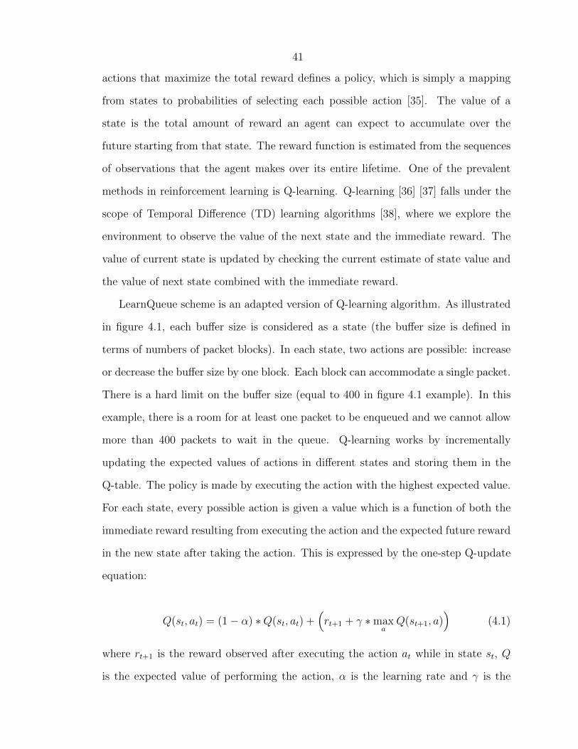
LearnQueue scheme is an adapted version of Q-learning algorithm. As illustrated
in figure 4.1, each buffer size is considered as a state (the buffer size is defined in
terms of numbers of packet blocks). In each state, two actions are possible: increase
or decrease the buffer size by one block. Each block can accommodate a single packet.
There is a hard limit on the buffer size (equal to 400 in figure 4.1 example). In this
example, there is a room for at least one packet to be enqueued and we cannot allow
more than 400 packets to wait in the queue. Q-learning works by incrementally
updating the expected values of actions in different states and storing them in the
Q-table. The policy is made by executing the action with the highest expected value.
For each state, every possible action is given a value which is a function of both the
immediate reward resulting from executing the action and the expected future reward
in the new state after taking the action. This is expressed by the one-step Q-update
equation:
Q(st, at) = (1− α) ∗Q(st, at) +(rt+1 + γ ∗max
aQ(st+1, a)
)(4.1)
where rt+1 is the reward observed after executing the action at while in state st, Q
is the expected value of performing the action, α is the learning rate and γ is the

42
Figure 4.1: Overview of LearnQueue design.
discount factor.
The discount factor γ determines the importance of future rewards. Thus, for the
sake of accelerating the learning process, we start with a low discount factor equal to
5 % and increase it with the number of the couples of action-state discovered towards
90 %.
4.2.2 Learning Process
Our algorithm should be completely goal-independent, allowing the mechanics of the
environment to be learned independently of the actions that are being undertaken.
In order to be goal-independent, the algorithm must also be policy-independent. Al-
though the Q-learning algorithm is independent of the policy [39], it is not goal-
independent. In our application, there exists no specific goal state to reach. Ad-
ditionally, the reward given by moving from one state to another is not predefined.
Moreover, the algorithm should be called periodically instead of running for a de-
fined number of iterations in order to keep adapting the queue length to the changing
network conditions. We modified the original Q-learning algorithm to meet those
requirements. The pseudocode of LearnQueue scheme is given in Algorithm 1 (see
Appendix A). Note that the algorithm was designed to cope with a system with
multiple queues being dequeued using a round-robin strategy. Also, we drew the
attention of the reader that the variable “queue size” controls the queue length ex-
43
pressed in number of packets. It includes both enqueued packets and empty slots. For
the sake of exploring the environment, our method makes use of adaptive ε-greedy
strategy for choosing actions. With a probability ε, we randomly select an action,
independently from the Q-values estimates. The exploration probability ε defines the
trade-off between discovering new possibilities (exploration) and refining current pro-
cedure (exploitation). We start by a high exploration probability ε = 0.9 and decrease
it non-linearly with the number of action-state combinations discovered towards its
final value ε = 0.1, thus ensuring optimal actions are discovered.
4.2.3 Reward Function
The learning process is governed by the reward function. The key challenge here
is to design a reward function that penalizes the actions resulting in longer delay
than a specified target without causing a significant increase in the dropping rate.
Indeed, there is a delicate balance between achieving low latency and maintaining
high enqueue rate. The reward function contains two components: “delay reward”
which is related to delay and “enq reward” which is related to dropping. The former
measures the deviation of the current queuing delay “curr delay” from the reference
latency value “delay ref” and calculated as:
delay reward = δ ∗ (delay ref − curr delay) (4.2)
The latter presents the enqueue rate scaled to the delay and calculated as:
enq reward = η ∗ (max delay − delay ref) ∗ enq rate (4.3)
where “enq rate” is computed by dividing the number of enqueued packets by the
total number of both enqueued and dropped packets over the update period of the
algorithm. “max delay” is the maximum required time to drain the queue calculated
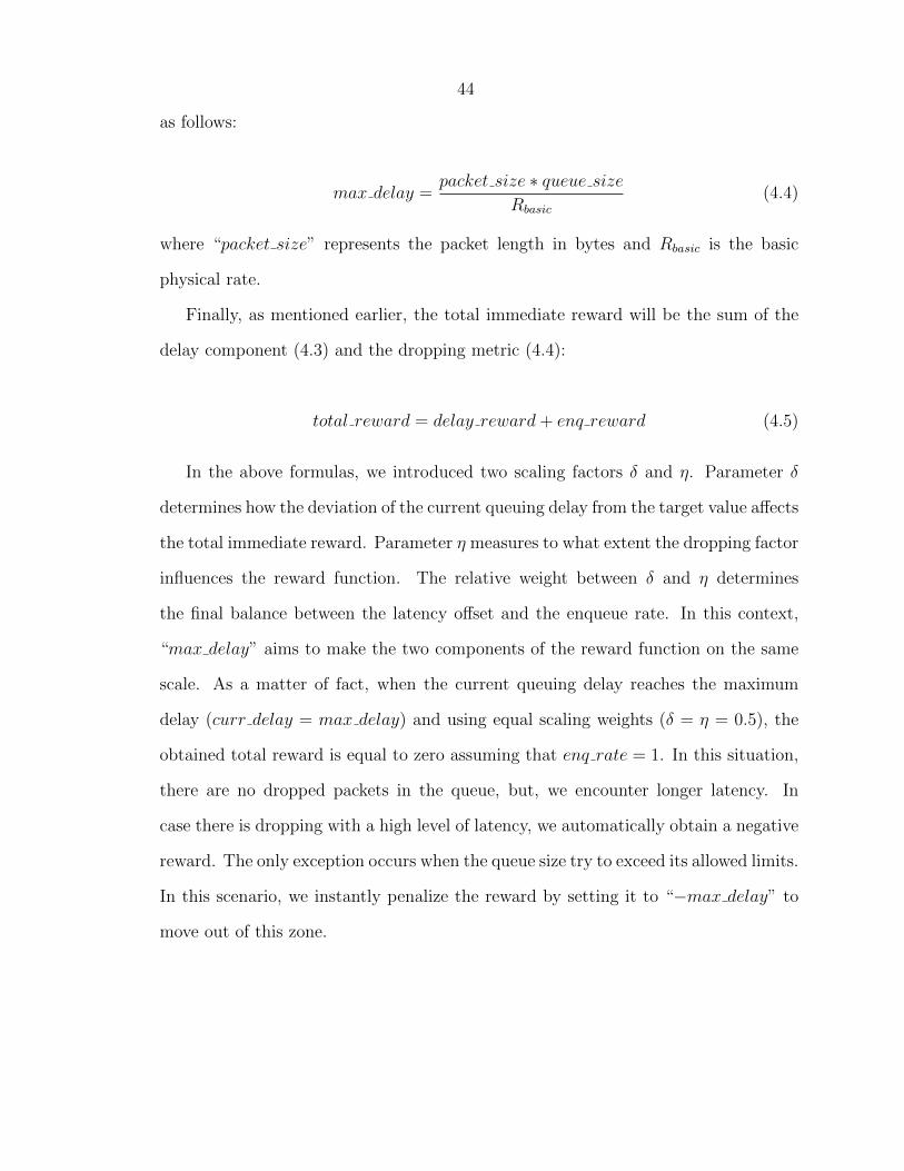
44
as follows:
max delay =packet size ∗ queue size
Rbasic
(4.4)
where “packet size” represents the packet length in bytes and Rbasic is the basic
physical rate.
Finally, as mentioned earlier, the total immediate reward will be the sum of the
delay component (4.3) and the dropping metric (4.4):
total reward = delay reward+ enq reward (4.5)
In the above formulas, we introduced two scaling factors δ and η. Parameter δ
determines how the deviation of the current queuing delay from the target value affects
the total immediate reward. Parameter η measures to what extent the dropping factor
influences the reward function. The relative weight between δ and η determines
the final balance between the latency offset and the enqueue rate. In this context,
“max delay” aims to make the two components of the reward function on the same
scale. As a matter of fact, when the current queuing delay reaches the maximum
delay (curr delay = max delay) and using equal scaling weights (δ = η = 0.5), the
obtained total reward is equal to zero assuming that enq rate = 1. In this situation,
there are no dropped packets in the queue, but, we encounter longer latency. In
case there is dropping with a high level of latency, we automatically obtain a negative
reward. The only exception occurs when the queue size try to exceed its allowed limits.
In this scenario, we instantly penalize the reward by setting it to “−max delay” to
move out of this zone.
45
4.3 Implementation
We have implemented our scheme using off-the-shelves WARP v3 boards [40]. We
modified the queuing system of the 802.11 Reference Design v1.6 [22]. The low-
level MAC of the reference design handles one packet at a time. The high-level MAC
manages many packets at once via a series of queues. In the reference implementation,
one queue is created per associated node plus one queue for all broadcast traffic and
one queue for all management packets. Whenever the low-level MAC finishes the
transmission of a packet, the next available packet is dequeued from the appropriate
queue and passed to CPU Low for transmission. The Access Point (AP) implements
a round-robin dequeuing procedure and alternates between different queues. When
new packet requiring wireless transmission is received, it will be added to the tail of
the queue associated with the node to which the packet is addressed. Similar to Wi-
Fi commercial devices, WARP v3 boards adopt Drop Tail as default queuing policy,
which means when the queue is filled to its maximum capacity, the newly arriving
packets are dropped until the queue has enough room to accept incoming traffic.
LearnQueue manages each queue independently from the others. We do not alter
multicast and management queues default behavior since our focus is only on data
frames queues. Our scheme is evaluated in a wireless testbed in our lab. The testbed
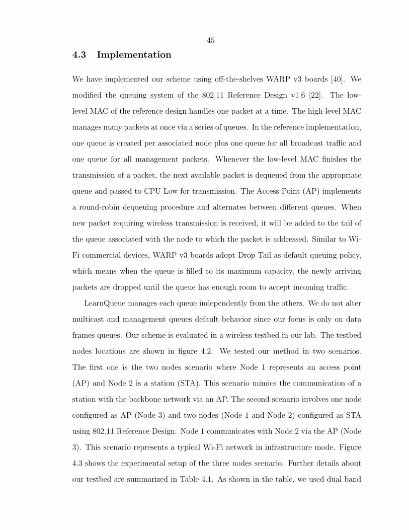
nodes locations are shown in figure 4.2. We tested our method in two scenarios.
The first one is the two nodes scenario where Node 1 represents an access point
(AP) and Node 2 is a station (STA). This scenario mimics the communication of a
station with the backbone network via an AP. The second scenario involves one node
configured as AP (Node 3) and two nodes (Node 1 and Node 2) configured as STA
using 802.11 Reference Design. Node 1 communicates with Node 2 via the AP (Node
3). This scenario represents a typical Wi-Fi network in infrastructure mode. Figure
4.3 shows the experimental setup of the three nodes scenario. Further details about
our testbed are summarized in Table 4.1. As shown in the table, we used dual band

46
Figure 4.2: The lab room plan showing testbed nodes locations.
omni-directional VERT 2450 antennas [41] for operation in the 5 GHz radio band to
avoid interference with our campus production network.
4.4 Performance Evaluation
In this section, we evaluate the performance of LearnQueue scheme in both two nodes
scenario and three nodes scenario. We choose to compare LearnQueue’s performance
Figure 4.3: Experimental setup of the three nodes scenario.

47
Table 4.1: Testbed parameters summary.
Parameter Value
Wi-Fi Standard IEEE 802.11nBasic Physical Rate 6.5 MbpsMaximum Physical Rate 65 MbpsRadio Band 5 GHzChannel 36TX Power 15 dBmPackets Size 1500 BytesMax Queue Size 400 packetsDistance Between Node 1 and Node 2 10 mDistance Between Node 1 and Node 3 7.3 mDistance Between Node 2 and Node 3 5.6 m
against a dropping-based method and a dynamic buffer sizing method. The most
recent state of the art methods are PIE and WQM discussed earlier. Those algorithms
are only implemented in Linux. Thus, we also implement both PIE and WQM in our
hardware. To the best of our knowledge, this is the first work that integrates AQM
techniques into WARP v3 boards instead of Linux devices. Unless otherwise stated,
all latency statistics are extracted from the sender node, and the experiments are done
using the physical rate of 26 Mbps. In all experiments, we set LearnQueue scaling
weights to their standard values δ = η = 0.5. PIE and WQM parameters are fixed
to their default values. However, for the sake of fair comparison, we define a unique
reference latency value for all the schemes (equal to 30 ms).
4.4.1 Two Nodes Scenario
To stress the queues inside our devices, we run a fully backlogged flow from the AP to
the STA for 100 s using a local Constant Bit Rate (CBR) traffic generator and measure
its queuing latency and throughput. We aim here to simulate a heavily congested
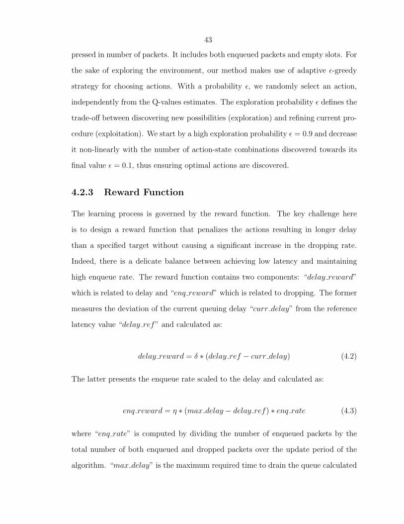
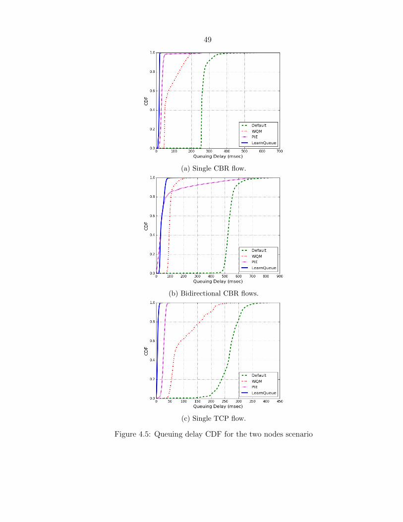
wireless link. Figure 4.5a plots the Cumulative Distribution Function (CDF) of the
queuing delay in the sender node for the four methods. More than 98 % of packets
under both LearnQueue and PIE experience less than 50 ms latency. But, it is clear
48
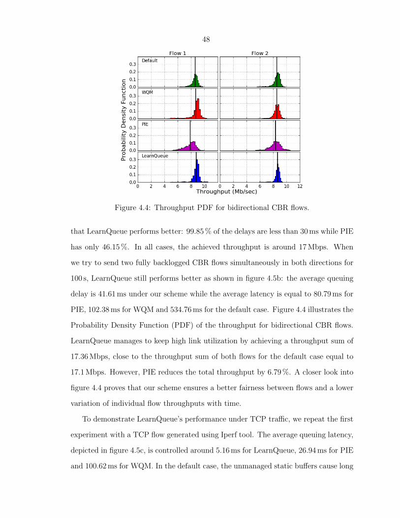
Figure 4.4: Throughput PDF for bidirectional CBR flows.
that LearnQueue performs better: 99.85 % of the delays are less than 30 ms while PIE
has only 46.15 %. In all cases, the achieved throughput is around 17 Mbps. When
we try to send two fully backlogged CBR flows simultaneously in both directions for
100 s, LearnQueue still performs better as shown in figure 4.5b: the average queuing
delay is 41.61 ms under our scheme while the average latency is equal to 80.79 ms for
PIE, 102.38 ms for WQM and 534.76 ms for the default case. Figure 4.4 illustrates the
Probability Density Function (PDF) of the throughput for bidirectional CBR flows.
LearnQueue manages to keep high link utilization by achieving a throughput sum of
17.36 Mbps, close to the throughput sum of both flows for the default case equal to
17.1 Mbps. However, PIE reduces the total throughput by 6.79 %. A closer look into
figure 4.4 proves that our scheme ensures a better fairness between flows and a lower
variation of individual flow throughputs with time.
To demonstrate LearnQueue’s performance under TCP traffic, we repeat the first
experiment with a TCP flow generated using Iperf tool. The average queuing latency,
depicted in figure 4.5c, is controlled around 5.16 ms for LearnQueue, 26.94 ms for PIE
and 100.62 ms for WQM. In the default case, the unmanaged static buffers cause long
49
(a) Single CBR flow.
(b) Bidirectional CBR flows.
(c) Single TCP flow.
Figure 4.5: Queuing delay CDF for the two nodes scenario
50
(a) Default (b) LearnQueue
Figure 4.6: Congestion window and Slow start threshold vs. Time
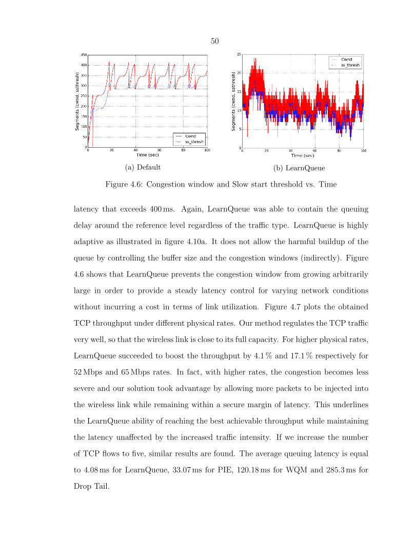
latency that exceeds 400 ms. Again, LearnQueue was able to contain the queuing
delay around the reference level regardless of the traffic type. LearnQueue is highly
adaptive as illustrated in figure 4.10a. It does not allow the harmful buildup of the
queue by controlling the buffer size and the congestion windows (indirectly). Figure
4.6 shows that LearnQueue prevents the congestion window from growing arbitrarily
large in order to provide a steady latency control for varying network conditions
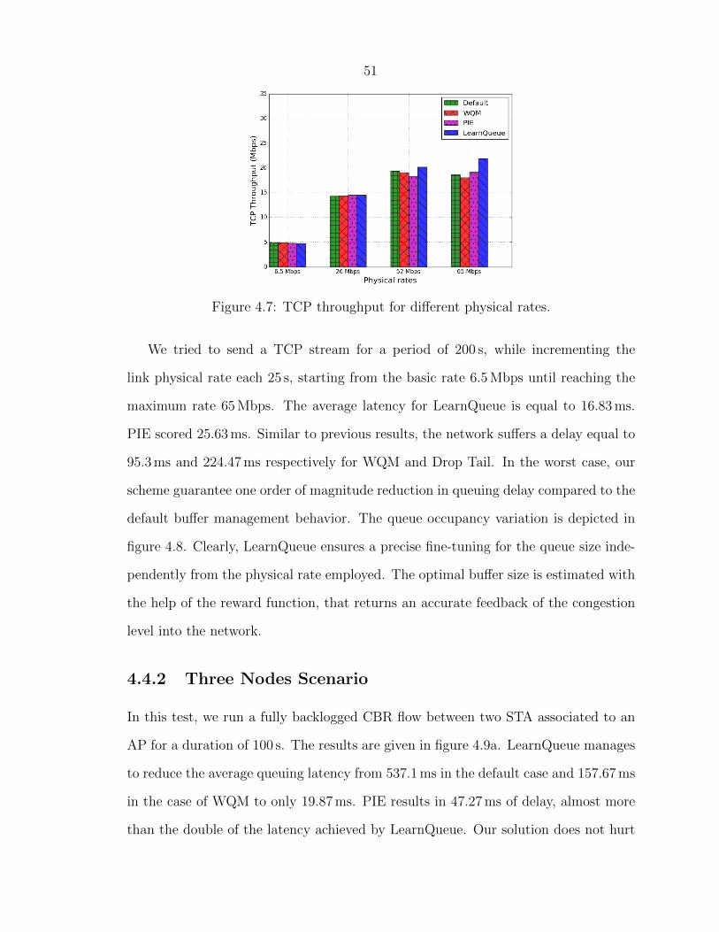
without incurring a cost in terms of link utilization. Figure 4.7 plots the obtained
TCP throughput under different physical rates. Our method regulates the TCP traffic
very well, so that the wireless link is close to its full capacity. For higher physical rates,
LearnQueue succeeded to boost the throughput by 4.1 % and 17.1 % respectively for
52 Mbps and 65 Mbps rates. In fact, with higher rates, the congestion becomes less
severe and our solution took advantage by allowing more packets to be injected into
the wireless link while remaining within a secure margin of latency. This underlines
the LearnQueue ability of reaching the best achievable throughput while maintaining
the latency unaffected by the increased traffic intensity. If we increase the number
of TCP flows to five, similar results are found. The average queuing latency is equal
to 4.08 ms for LearnQueue, 33.07 ms for PIE, 120.18 ms for WQM and 285.3 ms for
Drop Tail.
51
Figure 4.7: TCP throughput for different physical rates.
We tried to send a TCP stream for a period of 200 s, while incrementing the
link physical rate each 25 s, starting from the basic rate 6.5 Mbps until reaching the
maximum rate 65 Mbps. The average latency for LearnQueue is equal to 16.83 ms.
PIE scored 25.63 ms. Similar to previous results, the network suffers a delay equal to
95.3 ms and 224.47 ms respectively for WQM and Drop Tail. In the worst case, our
scheme guarantee one order of magnitude reduction in queuing delay compared to the
default buffer management behavior. The queue occupancy variation is depicted in
figure 4.8. Clearly, LearnQueue ensures a precise fine-tuning for the queue size inde-
pendently from the physical rate employed. The optimal buffer size is estimated with
the help of the reward function, that returns an accurate feedback of the congestion
level into the network.
4.4.2 Three Nodes Scenario
In this test, we run a fully backlogged CBR flow between two STA associated to an
AP for a duration of 100 s. The results are given in figure 4.9a. LearnQueue manages
to reduce the average queuing latency from 537.1 ms in the default case and 157.67 ms
in the case of WQM to only 19.87 ms. PIE results in 47.27 ms of delay, almost more
than the double of the latency achieved by LearnQueue. Our solution does not hurt

52
Figure 4.8: Queue occupancy when using multi physical rates.
the throughput since it achieves 8.97 Mbps, almost equal to the default throughput
(8.98 Mbps) while PIE slightly reduces the throughput to 8.89 Mbps. Considering
bidirectional flows, LearnQueue reduces the average queuing latency from 603.56 ms
in the default case and 183.73 ms in the case of PIE to only 60.19 ms. Compared to the
default case, this corresponds to 10x reduction, which is a significant improvement.
This time, in comparison to the default scheme, a small drop occurs in the network
throughput from 12.79 Mbps to 11.65 Mbps. However, LearnQueue still performing
better than PIE (11.24 Mbps) and WQM (11.44 Mbps).
The experiment is repeated using two bidirectional TCP flows. The latency CDF
curves are reported in figure 4.9c. In average, the packets experience a queuing delay

53
(a) Single CBR flow.
(b) Bidirectional CBR flows.
(c) Bidirectional TCP flows.
Figure 4.9: Queuing delay CDF for the three nodes scenario
equal to 5.61 ms for LearnQueue, 16.68 ms for PIE, 48.17 ms for WQM and 56.17 ms
for the static buffers. LearnQueue achieves 9.31 Mbps as throughput, almost the

54
(a) Two nodes - Single TCP flow (b) Three nodes - Two TCP flows
Figure 4.10: Queue occupancy vs. Time
same with Drop Tail (9.58 Mbps). Curiously, the latency results are considered lower
than expected. We investigate this issue and we found that there is limited queue
buildup even in the default case (see figure 4.10b), which can be explained by a higher
packet error rate in the wireless links. Certainly, higher interference will slow down
the sending rate of TCP, affecting the congestion level into the network. LearnQueue
interacts with the light traffic and allows for more packets to be enqueued (more than
65 packets in some cases as shown in figure 4.10b) while outperforming the other
techniques.
4.5 Conclusion
In this chapter, we introduced LearnQueue, a reinforcement learning based design
for controlling bufferbloat in wireless networks. The LearnQueue design periodically

55
tunes the queue size by predicting the reward or the penalty resulting from explored
actions along with exploiting the prior experience accumulated. LearnQueue is model-
free, and the learning process is fully automated. We conducted various experiments
in a real testbed to validate the performance of our scheme under realistic conditions
and with different traffic types. The testbed results demonstrate that our framework
can be trusted to mitigate the effects of bufferbloat in congested networks while being
conservative for links with high interference levels.

56
Chapter 5
Concluding Remarks
5.1 Summary
Wireless networking is expected to see a huge shift in the next few years. Mobiles
devices such as mobile phones and tablets are replacing the traditional desktops and
becoming primary computing devices. Most of our data and applications will live
in the cloud, and users will expect to have access to them anytime, anywhere. The
expansion of wireless usage has resulted in more demanding applications. As a result,
improving the performance of wireless systems such as latency and throughput seems
crucial for their development in the future. The past few years have witnessed a
significant increase in wireless data usage, and this trend is expected to continue in the
near future. Therefore, ubiquitous high-speed and low-latency wireless connectivity
is needed.
In this dissertation, we considered the problem of buffer management in wire-
less networks. We thoroughly investigated WQM’s behavior and performance over
bufferbloated wireless full-duplex networks. We revealed that the excessive buffers
hurt the optimal performance of full-duplex. We have demonstrated through simu-
lation that WQM can decrease the latency in a relay full-duplex 802.11 testbed by
two orders of magnitude. However, WQM still has some limitations. Indeed, it is
dependent from the Wi-Fi standard and the rate control algorithm which may differ
from one device to another. Besides, the algorithm is not highly responsive to sudden
changes. To overcome those issues, we come up with a novel reinforcement learn-
57
ing scheme, LearnQueue, which adapts the buffer size according to a learned policy
and a reward function based on a modified version of the Q-learning algorithm. We
have investigated LearnQueue performance in various scenarios with different trans-
port protocols. Experiment results show that our scheme reduces queening latency
drastically while preserving similar throughput in most of the cases.
The intellectual merit of this research is to contribute to the efforts of establish-
ing the milestone of next-generation wireless technology. Our work provides a good
starting point for employing artificial intelligence and machine learning techniques to
optimize wireless networks performance.
5.2 Future Work
The work presented in this thesis can be extended in the following directions:
5.2.1 Green Wireless Networking
The rapid adoption of smartphones and tablets is driving up the global energy con-
sumption of Information and Communication Technologies (ICT). According to a
recent study [42], the average annual power consumed by ICT reached the equivalent
of the power produced by 117 standard nuclear reactors. The network energy bill
represents about 10−15 % of the operational expense of telecommunication service
providers in mature markets and even up to 50 % in some developing markets. There
is no doubt that the network energy consumption significantly contributes to the
world emissions of greenhouse gasses. The energy challenge for ICT can only become
more stringent in the coming years if no specific action is taken. To realize the vi-
sion of energy efficient high-speed wireless connectivity, there is a pressing need to
develop reliable wireless systems that consume minimum energy. The investigation
of the effect of buffer management on the energy efficiency of wireless devices is one
of our future work targets. For instance, power-saving mechanisms can be combined
58
with the queuing routine in the transmission side. Typically, a radio is put to sleep
only when it has no packets to transmit. The transmit circuitry can be scheduled
in coordination with the AQM scheme to optimize the sleep time in accordance with
the on-going transmissions.
5.2.2 Real-Time Full-Duplex
In this work, we only tested AQM in wireless full-duplex using simulation. Buffer
management is implemented on high MAC layer. Most wireless full-duplex proposals
in the literature are pure physical layer designs. Moreover, the multiple access pro-
tocol CSMA/CA in the current 802.11 wireless networks is not suitable for operation
in full-duplex mode. As a future work, we will consider developing a real-time full-
duplex design along with a new MAC layer scheme that fully leverages full-duplex
capabilities to maximize network throughput and fairness while being backward com-
patible with existing large deployments of half-duplex wireless devices. The MAC
protocol needs to be redesigned to allow for simultaneous transmit and receive op-
erations without a significant increase in collisions while achieving close to optimal
channel capacity. Real-time full-duplex seems an ambitious project.
5.2.3 Impact of Buffering on Video Streaming
We thoroughly investigated the behavior of different buffering techniques using var-
ious transport protocols such as TCP and UDP. However, we did not focus on their
interaction with a specific application. Minimizing the buffer size will bring down the
latency, but, it can produce collateral problems for a video streaming application. In
fact, streaming video is sensitive to dropping and has strict packet loss requirements.
The acceptable packet loss should be between 1 % and 2.5 %. Higher dropping rate
in the transmit queue will automatically result in a poor video quality. For this pur-
pose, we intend to investigate the impact of buffering on video streaming applications.
59
One possible approach is to set the scaling weights of LearnQueue in a way to favor
enqueue rate over latency.
5.2.4 Buffer Management with Priority-Enabled Queues
To enhance the performance of AQM methods, we can place each flow on its own
queue and, then, use a scheduling algorithm like any variation of round-robin to select
which queue to dequeue from. A flow may be identified by application type, source
address, destination address, QoS metrics, etc. The AQM algorithm should be applied
separately to each queue. Alternatively, we can just use a scheduling algorithm to
insert incoming packets belonging to many active flows into their suitable positions
in one queue. In this case, we must pay attention to the possible conflicts between
AQM and the scheduler that mixes packets of competing flows in the same queue,
which acts to pace bursty flows and better fill the pipe.

60
REFERENCES
[1] “NS-3 Model Library.” [Online]. Available: https://www.nsnam.org/docs/
models/html/
[2] J. Gettys and K. Nichols, “Bufferbloat: Dark Buffers in the Internet,” Queue,
vol. 9, no. 11, pp. 40:40–40:54, Nov. 2011.
[3] “Average Historic Price of RAM, Statistic Brain Research Institute.” [Online].
Available: http://www.statisticbrain.com/average-historic-price-of-ram/
[4] “IEEE Standard for Information technology–Telecommunications and informa-
tion exchange between systems–Local and metropolitan area networks–Specific
requirements-Part 11: Wireless LAN Medium Access Control (MAC) and Phys-
ical Layer (PHY) Specifications Amendment 3: Enhancements for Very High
Throughput in the 60 GHz Band,” IEEE Std 802.11ad-2012 (Amendment to
IEEE Std 802.11-2012, as amended by IEEE Std 802.11ae-2012 and IEEE Std
802.11aa-2012), pp. 1–628, Dec 2012.
[5] M. Dischinger, A. Haeberlen, K. P. Gummadi, and S. Saroiu, “Characterizing
Residential Broadband Networks,” in Proceedings of the 7th ACM SIGCOMM
Conference on Internet Measurement, ser. IMC ’07, 2007.
[6] C. Kreibich, N. Weaver, B. Nechaev, and V. Paxson, “Netalyzr: Illuminating
the Edge Network,” in Proceedings of the 10th ACM SIGCOMM Conference on
Internet Measurement, ser. IMC ’10, 2010.
[7] H. Jiang, Y. Wang, K. Lee, and I. Rhee, “Tackling Bufferbloat in 3G/4G Net-
works,” in Proceedings of the 2012 Internet Measurement Conference, ser. IMC
’12, 2012.
[8] R. Pan, P. Natarajan, C. Piglione, M. S. Prabhu, V. Subramanian, F. Baker,
and B. VerSteeg, “PIE: A lightweight control scheme to address the bufferbloat
problem,” in 2013 IEEE 14th International Conference on High Performance
Switching and Routing (HPSR), July 2013.
[9] “How latency is killing online gaming.” [Online]. Available: http://venturebeat.
com/2016/04/17/how-latency-is-killing-online-gaming/

61
[10] D. B. Terry, V. Prabhakaran, R. Kotla, M. Balakrishnan, M. K. Aguilera, and
H. Abu-Libdeh, “Consistency-based Service Level Agreements for Cloud Stor-
age,” in Proceedings of the Twenty-Fourth ACM Symposium on Operating Sys-
tems Principles, ser. SOSP ’13, 2013.
[11] A. Showail, K. Jamshaid, and B. Shihada, “WQM: An Aggregation-aware Queue
Management Scheme for IEEE 802.11N Based Networks,” in Proceedings of the
2014 ACM SIGCOMM Workshop on Capacity Sharing Workshop, ser. CSWS
’14, 2014.
[12] B. Braden, D. Clark, J. Crowcroft, B. Davie, S. Deering, D. Estrin, S. Floyd,
V. Jacobson, G. Minshall, C. Partridge, L. Peterson, K. Ramakrishnan,
S. Shenker, J. Wroclawski, and L. Zhang, “Recommendations on Queue Man-
agement and Congestion Avoidance in the Internet,” RFC 2309, April 1998.
[13] S. Floyd and V. Jacobson, “Random Early Detection Gateways for Congestion
Avoidance,” IEEE/ACM Trans. Netw., vol. 1, no. 4, pp. 397–413, Aug. 1993.
[14] K. Nichols and V. Jacobson, “Controlling Queue Delay,” Queue, vol. 10, no. 5,
pp. 20:20–20:34, May 2012.
[15] T. Hoiland-Jorgensen, Battling Bufferbloat: An Experimental Comparison of
Four Approaches to Queue Management in Linux, 2012. [Online]. Available:
https://books.google.com.sa/books?id=X4KjnQAACAAJ
[16] T. B. Cardozo, A. P. C. da Silva, A. B. Vieira, and A. Ziviani, “Bufferbloat sys-
tematic analysis,” in 2014 International Telecommunications Symposium (ITS),
Aug 2014.
[17] “Prominent features in Linux 3.3.” [Online]. Available: https://kernelnewbies.
org/Linux 3.3
[18] J. I. Choi, M. Jain, K. Srinivasan, P. Levis, and S. Katti, “Achieving Single
Channel, Full Duplex Wireless Communication,” in Proceedings of the Sixteenth
Annual International Conference on Mobile Computing and Networking, ser. Mo-
biCom ’10, 2010.
[19] M. Jain, J. I. Choi, T. Kim, D. Bharadia, S. Seth, K. Srinivasan, P. Levis,
S. Katti, and P. Sinha, “Practical, Real-time, Full Duplex Wireless,” in Pro-
ceedings of the 17th Annual International Conference on Mobile Computing and
Networking, ser. MobiCom ’11, 2011.
[20] “Ettus Ressearch USRP.” [Online]. Available: https://www.ettus.com/product
62
[21] M. Duarte, A. Sabharwal, V. Aggarwal, R. Jana, K. K. Ramakrishnan, C. W.
Rice, and N. K. Shankaranarayanan, “Design and Characterization of a Full-
Duplex Multiantenna System for WiFi Networks,” IEEE Transactions on Ve-
hicular Technology, vol. 63, no. 3, pp. 1160–1177, March 2014.
[22] “WARP Project.” [Online]. Available: http://warpproject.org
[23] “CM-MMCX: WARP Clock Module with MMCX connectors.” [Online].
Available: https://www.mangocomm.com/products/modules/cm-mmcx
[24] S. S. Hong, J. Mehlman, and S. Katti, “Picasso: Flexible RF and Spectrum
Slicing,” in Proceedings of the ACM SIGCOMM 2012 Conference on Applica-
tions, Technologies, Architectures, and Protocols for Computer Communication,
ser. SIGCOMM ’12, 2012.
[25] D. Bharadia, E. McMilin, and S. Katti, “Full Duplex Radios,” in Proceedings
of the ACM SIGCOMM 2013 Conference on SIGCOMM, ser. SIGCOMM ’13,
2013.
[26] D. Bharadia and S. Katti, “Full Duplex MIMO Radios,” in Proceedings of the
11th USENIX Conference on Networked Systems Design and Implementation,
ser. NSDI’14, 2014.
[27] A. Showail, K. Jamshaid, and B. Shihada, “Buffer sizing in wireless networks:
challenges, solutions, and opportunities,” IEEE Communications Magazine,
vol. 54, no. 4, pp. 130–137, April 2016.
[28] “Implement wireless full-duplex communication in the ns-3 network simulator.”
[Online]. Available: https://github.com/yusuke-sugiyama/ns-3-fdwifi
[29] K. Tamaki, A. R. H., Y. Sugiyama, M. Bandai, S. Saruwatari, and T. Watanabe,
“Full Duplex Media Access Control for Wireless Multi-Hop Networks,” in 2013
IEEE 77th Vehicular Technology Conference (VTC Spring), June 2013.
[30] G. F. Riley and T. R. Henderson, “The ns-3 Network Simulator.” in Modeling and
Tools for Network Simulation, M. Wehrle, Klaus and J. Gross, Eds. Springer,
2010, pp. 15–34.
[31] “Reinventing Wireless LAN.” [Online]. Available: http://www.shihada.com/
node/106
[32] “IEEE Standard for Information technology–Telecommunications and informa-
tion exchange between systems Local and metropolitan area networks–Specific

63
requirements Part 11: Wireless LAN Medium Access Control (MAC) and Phys-
ical Layer (PHY) Specifications,” IEEE Std 802.11-2012 (Revision of IEEE Std
802.11-2007), pp. 1–2793, March 2012.
[33] M. Lacage, M. H. Manshaei, and T. Turletti, “IEEE 802.11 Rate Adaptation: A
Practical Approach,” in Proceedings of the 7th ACM International Symposium on
Modeling, Analysis and Simulation of Wireless and Mobile Systems, ser. MSWiM
’04, 2004.
[34] R. S. Sutton and A. G. Barto, Introduction to Reinforcement Learning, 1st ed.
Cambridge, MA, USA: MIT Press, 1998.
[35] C. Gaskett, D. Wettergreen, and A. Zelinsky, “Q-Learning in Continuous State
and Action Spaces,” in Proceedings of the 12th Australian Joint Conference on
Artificial Intelligence: Advanced Topics in Artificial Intelligence, ser. AI ’99,
1999.
[36] L. P. Kaelbling, M. L. Littman, and A. W. Moore, “Reinforcement Learning: A
Survey,” J. Artif. Int. Res., vol. 4, no. 1, pp. 237–285, May 1996.
[37] C. J. Watkins and P. Dayan, “Technical Note: Q-Learning,” Machine Learning,
vol. 8, no. 3, pp. 279–292, 1992.
[38] R. S. Sutton, “Learning to predict by the methods of temporal differences,”
Machine Learning, vol. 3, no. 1, pp. 9–44, 1988.
[39] R. Ollington and P. Vamplew, “Concurrent Q-learning: Reinforcement learning
for dynamic goals and environments,” Int. J. Intell. Syst., vol. 20, no. 10, pp.
1037–1052, 2005.
[40] “WARP v3 Kit.” [Online]. Available: https://www.mangocomm.com/products/
kits/warp-v3-kit
[41] “VERT2450 Antenna.” [Online]. Available: https://www.ettus.com/product/
details/VERT2450
[42] T. E. Klein and P. Richard, “ICT Energy Challenges, Impact and Solutions,”
in 19th International ICIN Conference - Innovations in Clouds, Internet and
Networks, March 2016.
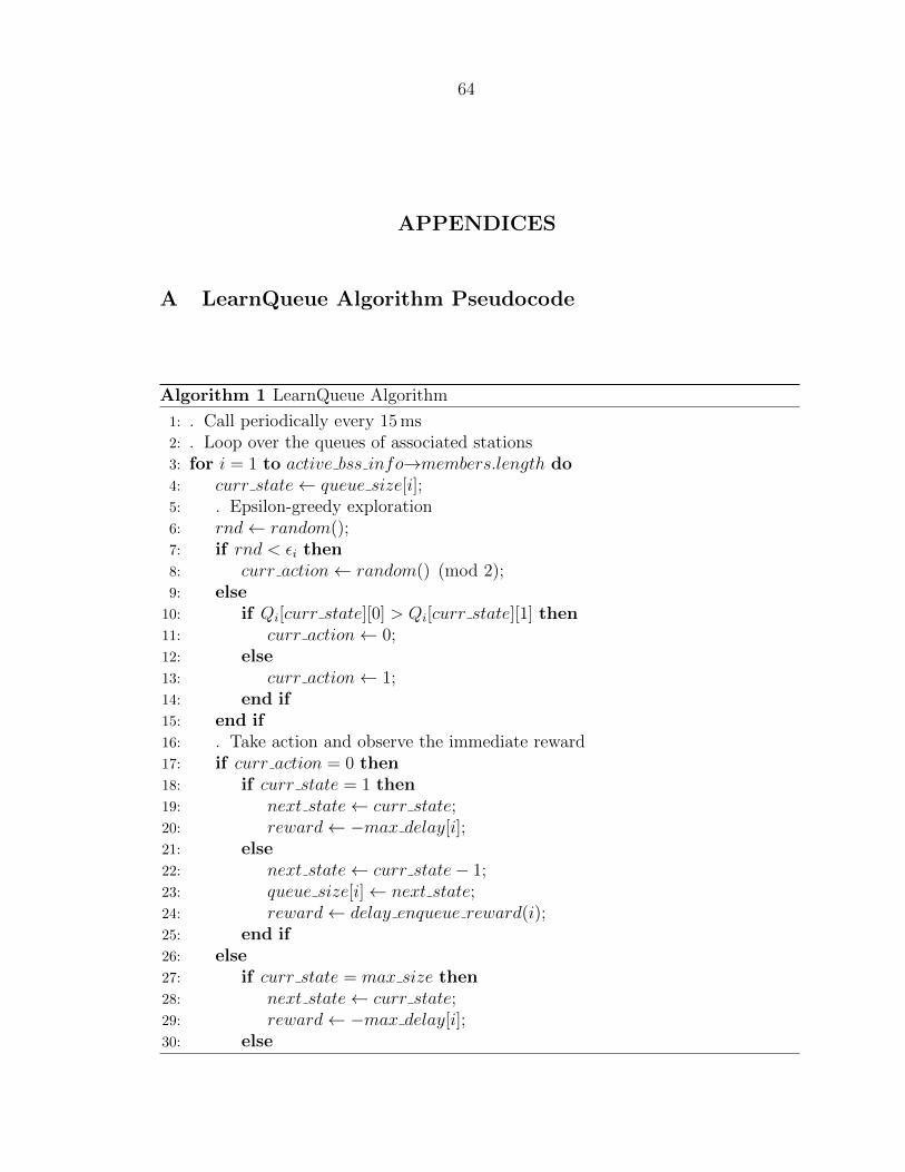
64
APPENDICES
A LearnQueue Algorithm Pseudocode
Algorithm 1 LearnQueue Algorithm
1: . Call periodically every 15 ms2: . Loop over the queues of associated stations3: for i = 1 to active bss info→members.length do4: curr state← queue size[i];5: . Epsilon-greedy exploration6: rnd← random();7: if rnd < εi then8: curr action← random() (mod 2);9: else
10: if Qi[curr state][0] > Qi[curr state][1] then11: curr action← 0;12: else13: curr action← 1;14: end if15: end if16: . Take action and observe the immediate reward17: if curr action = 0 then18: if curr state = 1 then19: next state← curr state;20: reward← −max delay[i];21: else22: next state← curr state− 1;23: queue size[i]← next state;24: reward← delay enqueue reward(i);25: end if26: else27: if curr state = max size then28: next state← curr state;29: reward← −max delay[i];30: else

65
31: queue size[i]← next state;32: reward← delay enqueue reward(i);33: end if34: end if35: . Tune exploration probability and discount factor36: if the state-action combination is not discovered then37: if εi > 0.1 then38: εi ← 0.995 ∗ εi;39: end if40: if γi < 0.9 then41: γi ← 1− (0.995 ∗ γi);42: end if43: end if44: . Update the Q-value for the current state-action45: s← curr state;46: a← curr action;47: Qi[s][a]← (1− α) ∗Qi[s][a] + (reward+ γi∗
max(Qi[next state][0], Qi[next state][1]));48: end for
66
B Papers Published and Under Review
• N. Bouacida, A. Showail and B. Shihada, “Buffer Management in Wireless Full-
Duplex Systems”, IEEE International Conference on Wireless and Mobile Computing,
Networking and Communications (WiMob), 2015.
• N. Bouacida, A. AlGhadhban, S. Al-Almaei, H. Mohammed and B. Shihada, “Fail-
ure Mitigation in Software Defined Networking Employing Load Type Prediction”,
Accepted in IEEE International Conference on Communications (ICC), 2017.
• N. Bouacida and B. Shihada, “LearnQueue: A Novel Reinforcement Learning
Scheme for Latency Control in Wireless Networks”, Submitted to IEEE Global Com-
munications Conference (GlobeCom), 2017.