Consist

ent *Complete *

Well D

ocumented*Easyt

oR

euse* *

Evaluated

*POPL*

Artifact

*AEC

Towards Automatic Resource Bound Analysis for OCaml

Jan Hoffmann Ankush DasCarnegie Mellon University

{jhoffmann, ankushd}@cs.cmu.edu

Shu-Chun WengYale University

scweng@gmail.com

AbstractThis article presents a resource analysis system for OCaml programs.The system automatically derives worst-case resource bounds forhigher-order polymorphic programs with user-defined inductivetypes. The technique is parametric in the resource and can derivebounds for time, memory allocations and energy usage. The derivedbounds are multivariate resource polynomials which are functionsof different size parameters that depend on the standard OCamltypes. Bound inference is fully automatic and reduced to a linearoptimization problem that is passed to an off-the-shelf LP solver.Technically, the analysis system is based on a novel multivariateautomatic amortized resource analysis (AARA). It builds on existingwork on linear AARA for higher-order programs with user-definedinductive types and on multivariate AARA for first-order programswith built-in lists and binary trees. This is the first amortizedanalysis, that automatically derives polynomial bounds for higher-order functions and polynomial bounds that depend on user-definedinductive types. Moreover, the analysis handles a limited form ofside effects and even outperforms the linear bound inference ofprevious systems. At the same time, it preserves the expressivityand efficiency of existing AARA techniques. The practicality ofthe analysis system is demonstrated with an implementation andintegration with Inria’s OCaml compiler. The implementation isused to automatically derive resource bounds for 411 functions and6018 lines of code derived from OCaml libraries, the CompCertcompiler, and implementations of textbook algorithms. In a casestudy, the system infers bounds on the number of queries that aresent by OCaml programs to DynamoDB, a commercial NoSQLcloud database service.

Categories and Subject Descriptors F.3.1 [Logics and Meaningsof Programs]: Specifying and Verifying and Reasoning about Pro-grams

General Terms Verification, Reliability

Keywords Resource Bound Analysis, Static Analysis, Type Sys-tems, Amortized Analysis, LP Solving, Type Inference

1. IntroductionThe quality of software crucially depends on the amount of resources—such as time, memory, and energy—that are required for its exe-cution. Statically understanding and controlling the resource usage

of software continues to be a pressing issue in software develop-ment. Performance bugs are very common and are among the bugsthat are most difficult to detect [40, 51]. Moreover, many securityvulnerabilities exploit the space and time usage of software [21, 42].

Developers would greatly profit from high-level resource-usageinformation in the specifications of software libraries and otherinterfaces, and from automatic warnings about potentially high-resource usage during code review. Such information is particularlyrelevant in contexts of mobile applications and cloud services, whereresources are limited or resource usage is a major cost factor.

Recent years have seen fast progress in developing frameworksfor statically reasoning about the resource usage of programs. Manyadvanced techniques for imperative integer programs apply abstractinterpretation to generate numerical invariants. The obtained size-change information forms the basis for the computation of actualbounds on loop iterations and recursion depths; using counterinstrumentation [27], ranking functions [2, 6, 15, 53], recurrencerelations [3, 4], and abstract interpretation itself [18, 60]. Automaticresource analysis techniques for functional programs are based onsized types [56], recurrence relations [23], term-rewriting [10], andamortized resource analysis [31, 34, 41, 52].

Despite major steps forward, there are still many obstacles toovercome to make resource analysis available to developers. On theone hand, typed functional programs are particularly well-suited forautomatic resource-bound analysis since the use of pattern matchingand recursion often results in a relatively regular code structure.Moreover, types provide detailed information about the shape ofdata structures. On the other hand, existing automatic techniques forhigher-order programs can only infer linear bounds [41, 56] or relyon defunctionalization [10]. Furthermore, techniques that can derivepolynomial bounds are limited to bounds that depend on predefinedlists and binary trees [29, 31], or integers [15, 53]. Finally, resourceanalyses for functional programs have been implemented for customlanguages that are not supported by mature tools for compilationand development [10, 31, 34, 41, 52, 56].

The goal of a long term research effort is to overcome theseobstacles by developing Resource Aware ML (RAML), a resource-aware version of the functional programming language OCaml.RAML is based on an automatic amortized resource analysis(AARA) that derives multivariate polynomials that are functions ofthe sizes of the inputs. In this paper, we report three research resultsthat are part of this effort.

1. We present the first implementation of an AARA that is inte-grated with an industrial-strength compiler.

2. We develop the first automatic resource analysis that infersmultivariate polynomial bounds that depend on size parametersof user-defined tree-like data structures.

3. We present the first AARA that infers polynomial bounds forhigher-order functions.

The techniques we develop are not tied to a particular resource butare parametric in the resource of interest. RAML infers tight bounds

for many complex example programs such as sorting algorithms withcomplex comparison functions, Dijkstra’s shortest-path algorithm,and the most common higher-order functions such as sequences ofnested maps, and folds. The technique is naturally compositional,tracks size changes of data across function boundaries, and can dealwith amortization effects that arise, for instance, from the use of afunctional queue. Local inference rules generate linear constraintsand reduce bound inference to off-the-shelf linear program (LP)solving, despite deriving polynomial bounds.

To ensure compatibility with OCaml’s syntax, we reuse the parserand type inference engine from Inria’s OCaml compiler [48]. Weextract a type-annotated syntax tree to perform (resource preserving)code transformations and the actual resource-bound analysis. Toprecisely model the evaluation of OCaml, we introduce a noveloperational semantics that makes the efficient handling of functionclosures in Inria’s compiler explicit. It can be seen as a big-stepformulation of the ZINC abstract machine [45]. The semantics iscomplemented by a new type system that refines function types.

To express a wide range of bounds, we introduce a novel class ofmultivariate resource polynomials that map data of a given type to anon-negative number. The set of multivariate resource polynomialsthat is available for bound inference depends on the types of inputdata. It can be parametric in (non-negative) integers, lengths of lists,or the number of particular nodes in an inductive data structure.As a special case, a resource polynomial can contain conditionaladditive factors. These novel multivariate resource polynomials are ageneralization of the resource polynomials that have been previouslydefined for lists and binary trees [31].

To deal with realistic OCaml code, we develop a novel multivari-ate AARA that handles higher-order functions. To this end, we drawinspirations from multivariate AARA for first-order programs [31]and linear AARA for higher-order programs [41]. However, our newsolution is more than the combination of existing techniques. Forinstance, we infer linear bounds for the curried append function forlists, which was not previously possible [41]. Moreover, we addressspecifics of Inria’s OCaml compiler such as efficiently avoidingfunction-closure creation.

OCaml is a complex language and resource bound analysis is anundecidable problem. As a result, there are many programs for whichRAML cannot derive bounds. We currently do not support severalOCaml features such as modules, object-oriented features, records,calls to native libraries, nested patterns, and optional arguments.The resource analysis is limited to polynomial bounds that dependon the sizes of inductive data structures that have nodes with fixedbranching factors. RAML can derive bounds for programs withexceptions, references, and arrays. However, we do not supportexception handlers and cannot derive bounds that depend on thesizes of data structures that are stored in arrays or references.

We performed experiments on more than 6018 lines of OCamlcode. Since RAML does not support some language features ofOCaml, it is not straightforward to automatically analyze completeexisting applications. However, the automatic analysis performs wellon code that only uses supported language features. For instance,we applied RAML to OCaml’s standard list library list.ml: RAMLautomatically derives evaluation-step bounds for 47 of the 51 top-level functions. All derived bounds are asymptotically tight.

It is also easy to develop and analyze real OCaml applications ifwe keep the current capabilities of the system in mind. In Section 9,we present a case study in which we automatically bound the numberof queries that an OCaml program issues to Amazon’s DynamoDBNoSQL cloud database service. Such bounds are interesting sinceAmazon charges DynamoDB users based on the number of queriesmade to the database.

Our experiments are easily reproducible: The source code ofRAML, the OCaml code for the experiments, and an easy-to-use

type (’a,’b) ablist = Acons of ’a * (’a,’b) ablist| Bcons of ’b * (’a,’b) ablist| Nil

let rec abmap f g abs = match abs with| Acons (a,abs’) → Acons(f a, abmap f g abs’)| Bcons (b,abs’) → Bcons(g b, abmap f g abs’)| Nil → Nil

let asort gt abs =abmap (quicksort gt) (fun x → x) abs

let asort’ gt abs =abmap (quicksort gt) (fun _ → raise Inv_arg) abs

let btick =abmap (fun a → a) (fun b → Raml.tick 2.5; b)

Excerpt of the RAML output for analyzing evaluation steps:

Simplified bound for abmap:3 + 12*L + 12*N

Simplified bound for asort:11 + 22*K*N + 13*K^2*N + 13*L + 15*N

Simplified bound asort’:13 + 22*K*N + 13*K^2*N + 15*N

Figure 1. Example bound analysis with RAML (0.23s run time).When reporting the linear bound for abmap to the user, we assumethat the higher-order arguments f and g have no resource consump-tion. L is the number of B-nodes, N is the number of A-nodes, andK is the maximal length of the lists in the A-nodes in the function’sarguments.

interactive web interface are available online [28]. The reviewersof the POPL’17 Artifact Evaluation found that RAML exceededor greatly exceeded their expectations. All technical details of thetheoretical development and an extensive description of the results ofthe experiments are available in a companion technical report [33].

2. OverviewBefore we describe the technical development, we give an overviewof the challenges and achievements of our work.

Example Bound Analysis. To demonstrate user interaction withRAML, Figure 1 contains an example bound analysis. The OCamlcode in Figure 1 will serve as a running example in this article. Thefunction abmap is a polymorphic map function for a user-definedlist that contains Acons and Bcons nodes. It takes two functions fand g as arguments and applies f to data stored in the A-nodes and gto data stored in the B-nodes. The function asort takes a comparisonfunction and an A-B-list in which the A-nodes contain lists. It thenuses quicksort (the code of quicksort is also automatically analyzedand available online [28]) to sort the lists in the A-nodes. The B-nodes are left unchanged. The function asort’ is a variation of asortthat raises an exception if it encounters a B-node in the list.

To derive a worst-case resource bound with RAML, the userneeds to pick a maximal degree of the search space of polynomialsand a resource metric. In the example analysis in Figure 1 we pickeddegree 4 and the steps metric which counts the number of evaluationsteps in the big-step semantics. RAML reports a bound for all top-level functions in 0.23 seconds. The shown output is only an excerpt.In this case, all derived bounds are tight in the sense that there areinputs for every size that exactly result in the reported number ofevaluation steps.

In the derived bound for abmap, RAML assumes that theresource cost of f and g is 0. So we get a linear bound. In thecase of asort we derive a bound which is quadratic in the maximallength of the lists that are stored in the A-nodes (22K + 13K2) forevery A-node in the list ((22K+13K2)N ) plus an additional linear

factor that also depends on the number of B-nodes that are simplytraversed (13L+ 15N ). For asort’ this linear factor only dependson the number of A-nodes: RAML automatically deduces that thetraversal is aborted in case we encounter a B-node.

The tick metric can be used to derive bounds on user definedmetrics. An instructive example is the function btick. With the tickmetric, RAML derives the bound 2.5L where L is the number ofB-nodes in the argument list. This is a tight bound on the sum of“ticks” that are executed in an evaluation of btick. Ticks can also benegative to express that resources become available.

Automatic Amortized Resource Analysis. The automatic resourceanalysis system of RAML is based on the potential method ofamortized analysis [54]. The idea is to introduce potential functionsthat depend on data structures. At every point in the program, theavailable potential needs to be sufficient to pay for the cost of thenext evaluation step and the potential at the next program point.

To be able to automate the analysis, we fix a set of possiblepotential functions for every data type. In RAML, potential functionsare non-negative linear combinations of a set of base polynomials.We integrate the coefficients of these linear combinations into atype system for OCaml. To this end, we use annotated types (A,Q)in which A is a standard type1 and Q is a family of non-negativecoefficients; one for every base polynomial. Given a value a oftype A, we define the potential Φ(a:(A,Q)) as a sum

∑i qi·pi(a)

where qi ranges over the coefficients in Q and pi ranges overthe base polynomials for type A. The type rules of RAML’s typesystem manipulate the coefficients Q to ensure correct accountingas potential is assigned to new data structures or used to pay forresource usage. The advantage of this setup is that we can expressthe relationships between different type annotations with linearconstraints. They can be collected during type inference and solvedby linear programming in a similar way as ordinary type constraintsare collected to be solved by unification.

Multivariate Resource Polynomials. Existing AARA systems areeither limited to linear bounds [34, 41] or to polynomial bounds thatare functions of the sizes of simple predefined lists and binary-treedata structures [31]. In contrast, this work presents the first analysisthat can derive polynomial bounds that depend on size parametersof complex user-defined data structures.

Consider for example the function btick of type (α∗β) ablist→(α ∗ β) ablist in Figure 1. The base polynomials for the argumentinclude

(mi

)·(nj

)where m denotes the number of A-nodes and n

denotes the number of B-nodes in the argument abs.2 The derivedbound 2.5n is represented by

∑i,j q(i,j)

(mi

)(nj

)where q(0,1) = 2.5

and q(i,j) = 0 otherwise. The corresponding function type is

btick : ((α ∗ β) ablist, Q)→ ((α ∗ β) ablist, P )

where Q contains the coefficients q(i,j), P contains coefficientsp(i,j), and p(i,j) = 0 for all (i, j). This reflects the fact that theinitial potential 2.5n is used up after the evaluation of btick.

Depending on the call side of btick, we might need differentpotential annotations P and Q. Usually, we pass on some potentialfrom the argument to the result of a function so that it can beconsumed in the remainder of the evaluation. Consider for examplethe inner call to btick in an expression like btick(btick abs). Here, weneed to cover the cost of the inner call (2.5n) and pass potential onto the resulting list (2.5n). This is reflected by a potential annotationin which q(0,1) = 5 and p(0,1) = 2.5.

In general, the bounds we derive are multivariate resourcepolynomials that can take into account individual sizes of inner data

1 This is not true in general since A can contain annotated function types butit is a good approximation to get a first impression.2 To be precise, these functions are sums of base polynomials.

structures. While it is possible to simplify the resource polynomialsin the user output, it is essential to have this more precise informationfor intermediate results to derive tight whole-program bounds. Ingeneral, the resource bounds are built of functions that count thenumber of specific tuples that one can form from the nodes in a tree-like data structure. In their simplest form (i.e., without consideringthe data stored inside the nodes), they have the form

λa.|{~a | ai is an Aki -node in a and if i < j then ai <apre aj}|

where a is an inductive data structure with constructorsA1, . . . , Am,~a = (a1, . . . , an), and <apre denotes the pre-order (tree traversal)on the tree a. For example, consider the aforementioned polynomialn·m for values of type ablist where m and n are the number A-and B-nodes, respectively. This is in fact the sum of the two basepolynomials λ`.|{(a, b) | a <`pre b}| and λ`.|{(b, a) | b <`pre a}|for A-B-lists (a ranges over A-nodes and b ranges over B-nodes).

We are able to keep track of changes of these quantities in patternmatches and data construction fully automatically by generatinglinear constraints. At the same time, they allow us to accuratelydescribe the resource usage of many common functions in thesame way it has been done previously for simple types [31]. Asan interesting special case, we can also derive bounds that describethe resource usage as a conditional statement. For instance, for anexpression such as

match x with | true → quicksort y | false → y

we derive a bound that is quadratic in the length of y if x is True andconstant if x is False.

Currying and Function Closures. Currying and function closurespose a challenge to automatic resource analysis systems that hasnot been addressed in the past. To see why, assume that we wantto design a type system to verify resource usage. Now consider forexample the curried append function which has the type append :α list → α list → α list in OCaml. At first glance, we might saythat the time complexity of append is O(n) if n is the length of thefirst argument. But a closer inspection of the definition of appendreveals that this is a gross simplification. In fact, the complexity ofthe partial function call app_par = append ` is constant. Moreover,the complexity of the function app_par is linear—not in the lengthof the argument but in the length of the list ` that is captured in thefunction closure. We are not aware of any existing approach that canautomatically derive a worst-case time bound for the curried appendfunction. For example, previous AARA systems would fail withoutderiving a bound [31, 41].

In general, we have to describe the resource consumption of acurried function f : A1 → · · · → An → A with n expressionsci(a1, . . . , ai) such that ci describes the complexity of the compu-tation that takes place after f is applied to i arguments a1, . . . , ai.In Inria’s OCaml implementation, the situation is even more com-plex since the resource usage (time and space) depends on how afunction is used at its call sites. If append is partially applied to oneargument then a function closure is created as expected. However,if append is applied to both of its arguments at the same time thenthe intermediate closure is not created and the performance of thefunction is even better than that of the uncurried version since wedo not have to create a pair before the application.

To model the resource usage of curried functions accurately,we refine function types to capture how functions are used attheir call sites. For example, append can have both of the typesα list → α list → α list and [α list, α list] → α list. The firsttype implies that the function is partially applied and the secondtype implies that the function is applied to both arguments at thesame time. Of course, it is possible that the function has both types(technically we achieve this using let polymorphism). For the secondtype, our system automatically derives tight time and space bounds

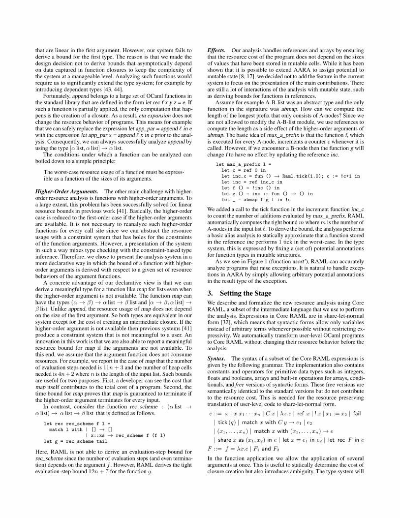
that are linear in the first argument. However, our system fails toderive a bound for the first type. The reason is that we made thedesign decision not to derive bounds that asymptotically dependon data captured in function closures to keep the complexity ofthe system at a manageable level. Analyzing such functions wouldrequire us to significantly extend the type system; for example byintroducing dependent types [43, 44].

Fortunately, append belongs to a large set of OCaml functions inthe standard library that are defined in the form let rec f x y z = e. Ifsuch a function is partially applied, the only computation that hap-pens is the creation of a closure. As a result, eta expansion does notchange the resource behavior of programs. This means for examplethat we can safely replace the expression let app_par = append ` in ewith the expression let app_par x = append ` x in e prior to the anal-ysis. Consequently, we can always successfully analyze append byusing the type [α list, α list]→ α list.

The conditions under which a function can be analyzed canboiled down to a simple principle:

The worst-case resource usage of a function must be express-ible as a function of the sizes of its arguments.

Higher-Order Arguments. The other main challenge with higher-order resource analysis is functions with higher-order arguments. Toa large extent, this problem has been successfully solved for linearresource bounds in previous work [41]. Basically, the higher-ordercase is reduced to the first-order case if the higher-order argumentsare available. It is not necessary to reanalyze such higher-orderfunctions for every call site since we can abstract the resourceusage with a constraint system that has holes for the constraintsof the function arguments. However, a presentation of the systemin such a way mixes type checking with the constraint-based typeinference. Therefore, we chose to present the analysis system in amore declarative way in which the bound of a function with higher-order arguments is derived with respect to a given set of resourcebehaviors of the argument functions.

A concrete advantage of our declarative view is that we canderive a meaningful type for a function like map for lists even whenthe higher-order argument is not available. The function map canhave the types (α → β) → α list → β list and [α → β, α list] →β list. Unlike append, the resource usage of map does not dependon the size of the first argument. So both types are equivalent in oursystem except for the cost of creating an intermediate closure. If thehigher-order argument is not available then previous systems [41]produce a constraint system that is not meaningful to a user. Aninnovation in this work is that we are also able to report a meaningfulresource bound for map if the arguments are not available. Tothis end, we assume that the argument function does not consumeresources. For example, we report in the case of map that the numberof evaluation steps needed is 11n+ 3 and the number of heap cellsneeded is 4n+2 where n is the length of the input list. Such boundsare useful for two purposes. First, a developer can see the cost thatmap itself contributes to the total cost of a program. Second, thetime bound for map proves that map is guaranteed to terminate ifthe higher-order argument terminates for every input.

In contrast, consider the function rec_scheme : (α list →α list)→ α list→ β list that is defined as follows.

let rec rec_scheme f l =match l with | [] → []

| x::xs → rec_scheme f (f l)let g = rec_scheme tail

Here, RAML is not able to derive an evaluation-step bound forrec_scheme since the number of evaluation steps (and even termina-tion) depends on the argument f . However, RAML derives the tightevaluation-step bound 12n+ 7 for the function g.

Effects. Our analysis handles references and arrays by ensuringthat the resource cost of the program does not depend on the sizesof values that have been stored in mutable cells. While it has beenshown that it is possible to extend AARA to assign potential tomutable state [8, 17], we decided not to add the feature in the currentsystem to focus on the presentation of the main contributions. Thereare still a lot of interactions of the analysis with mutable state, suchas deriving bounds for functions in references.

Assume for example A-B-list was an abstract type and the onlyfunction in the signature was abmap. How can we compute thelength of the longest prefix that only consists of A-nodes? Since weare not allowed to modify the A-B-list module, we use references tocompute the length as a side effect of the higher-order arguments ofabmap. The basic idea of max_a_prefix is that the function f, whichis executed for every A-node, increments a counter c whenever it iscalled. However, if we encounter a B-node then the function g willchange f to have no effect by updating the reference inc.

let max_a_prefix l =let c = ref 0 inlet inc_c = fun () → Raml.tick(1.0); c := !c+1 inlet inc = ref inc_c inlet f () = !inc () inlet g () = inc := fun () → () inlet _ = abmap f g l in !c

We added a call to the tick function in the increment function inc_cto count the number of additions evaluated by max_a_prefix. RAMLautomatically computes the tight boundmwherem is the number ofA-nodes in the input list `. To derive the bound, the analysis performsa basic alias analysis to statically approximate that a function storedin the reference inc performs 1 tick in the worst-case. In the typesystem, this is expressed by fixing a (set of) potential annotationsfor function types in mutable structures.

As we see in Figure 1 (function asort’), RAML can accuratelyanalyze programs that raise exceptions. It is natural to handle excep-tions in AARA by simply allowing arbitrary potential annotationsin the result type of the exception.

3. Setting the StageWe describe and formalize the new resource analysis using CoreRAML, a subset of the intermediate language that we use to performthe analysis. Expressions in Core RAML are in share-let-normalform [32], which means that syntactic forms allow only variablesinstead of arbitrary terms whenever possible without restricting ex-pressivity. We automatically transform user-level OCaml programsto Core RAML without changing their resource behavior before theanalysis.

Syntax. The syntax of a subset of the Core RAML expressions isgiven by the following grammar. The implementation also containsconstants and operators for primitive data types such as integers,floats and booleans, arrays and built-in operations for arrays, condi-tionals, and free versions of syntactic forms. These free versions aresemantically identical to the standard versions but do not contributeto the resource cost. This is needed for the resource preservingtranslation of user-level code to share-let-normal form.

e ::= x | x x1 · · ·xn | C x | λx.e | ref x | !x | x1 := x2 | fail| tick (q) | match x with C y → e1 | e2

| (x1, . . . , xn) | match x with (x1, . . . , xn)→ e

| share x as (x1, x2) in e | let x = e1 in e2 | let rec F in e

F ::= f = λx.e | F1 and F2

In the function application we allow the application of severalarguments at once. This is useful to statically determine the cost ofclosure creation but also introduces ambiguity. The type system will

S 6= · H(`) = (λx.e, V ′) V (x1):: · · · ::V (xn), V,HM`x ⇓ ` | (q, q′) S, V ′, HM`λx.e ⇓ w | (p, p′)S, V,HM`x x1 · · ·xn ⇓ w |Mapp

n ·(q, q′)·(p, p′)(E:APPAPP)

V (x1):: · · · ::V (xn), V,HM`x ⇓ w | (q, q′)·, V,HM`x x1 · · ·xn ⇓ w |Mapp

n ·(q, q′)(E:APP)

S 6= · H(V (x)) = (λx.e, V ′) S, V ′, HM`λx.e ⇓ w | (q, q′)S, V,HM`x ⇓ w |Mvar·(q, q′)

(E:VARAPP)

V (x) = `

·, V,HM`x ⇓ (`,H) |Mvar (E:VAR)S, V [x 7→ `], HM` e ⇓ w | (q, q′)

`::S, V,HM`λx.e ⇓ w |Mbind·(q, q′)(E:ABSBIND)

H′ = H, ` 7→ (λx.e, V )

·, V,HM`λx.e ⇓ (`,H′) |Mabs(E:ABSCLOS)

Figure 2. Selected rules of the operational big-step semantics.

determine if an expression like f x1 x2 is parsed as (f x1 x2) or(f x1) x2. The sharing expressions share x as (x1, x2) in e is notstandard and used to explicitly introduce multiple occurrences of avariable. It binds the free variables x1 and x2 in e. The expressionfail is used to raise exceptions. The expression tick(q) contains afloating point constant q. It can be used with the tick metric tospecify a constant cost. A negative floating point number q meansthat resources become available.

Big-Step Operational Cost Semantics. The resource usage ofRAML programs is defined by a big-step operational cost semantics.The semantics has three interesting non-standard features. First, itmeasures (or defines) the resource consumption of the evaluationof a RAML expression by using a resource metric that defines aconstant cost for each evaluation step. If this cost is negative thenresources are returned. Second, it models terminating and divergingexecutions by inductively describing finite subtrees of infiniteexecution trees. Third, it models OCaml’s stack-based mechanismfor function application, which avoids creation of intermediatefunction closure, similar to the ZINC abstract machine (ZAM) [45].

Since we also consider resources like memory that can becomeavailable during an evaluation, we have to track the high-water markof the resource usage, that is, the maximal number of resource unitsthat are simultaneously used during an evaluation. To derive a high-water mark of a sequence of evaluations from the high-water marksof the sub evaluations one has to also take into account the numberof resource units that are available after each sub evaluation.

Figure 2 contains selected big-step operational evaluation rules.They define an evaluation judgment of the form

S, V,H M` e ⇓ (`,H ′) | (q, q′) .

It expresses the following. If the resource metric M , the argumentstack S, the environment V , and the initial heap H are given thenthe expression e evaluates to the location ` and the new heap H ′.The evaluation of e needs q ∈ Q+

0 resource units (high-water mark)and after the evaluation there are q′ ∈ Q+

0 resource units available.The actual resource consumption is then δ = q − q′. The quantity δis negative if resources become available during the execution of e.

There are two other behaviors that we have to express in thesemantics: failure (i.e., array access outside array bounds) anddivergence. To this end, our semantic judgement not only evaluatesexpressions to values but also to an error ⊥ and to incompletecomputations expressed by ◦. The judgement has the general form

S, V,H M` e ⇓ w | (q, q′) where w ::= (`,H) | ⊥ | ◦ .

Intuitively, this evaluation statement expresses that the high-watermark of the resource consumption after some number of evaluationsteps is q and there are currently q′ resource units left. A resourcemetric M : K × N → Q defines the resource consumption ineach evaluation step of the big-step semantics where K is the set ofsyntactic forms. We write Mk

n for M(k, n) and Mk for M(k, 0).

The parameter n can be used to express the cost for steps that havedifferent costs for different types (e.g., creating an n-tuple).

It is handy to view the pairs (q, q′) in the evaluation judgmentsas elements of a monoidQ = (Q+

0 ×Q+0 , ·). The neutral element

is (0, 0), which means that resources are neither needed beforethe evaluation nor returned after the evaluation. The operation(q, q′) · (p, p′) defines how to account for an evaluation consistingof evaluations whose resource consumptions are defined by (q, q′)and (p, p′), respectively. We define

(q, q′) · (p, p′) =

{(q + p− q′, p′) if q′ ≤ p(q, p′ + q′ − p) if q′ > p

If resources are never returned (as with time) then we only haveelements of the form (q, 0) and (q, 0) · (p, 0) is just (q + p, 0). Weidentify a rational number q with an element ofQ as follows: q ≥ 0denotes (q, 0) and q < 0 denotes (0,−q). This notation avoidscase distinctions in the evaluation rules since the constants MK thatappear in the rules can be negative.

For efficiency reasons, Inria’s OCaml compiler evaluates func-tion applications e e1 · · · en from right to left, that is, it starts withevaluating en. In this way, one can avoid the expensive creationof intermediate function closures. A naive implementation wouldcreate n function closures when evaluating the aforementioned ex-pression: one for e, one for the application to the first argument, etc.By starting with the last argument, we are able to put the resultsof the evaluation on an argument stack and access them when weencounter a function abstraction during the evaluation. In this case,we do not create a closure but simply bind the value on the stack tothe name in the abstraction.

In the rules in Figure 2, we use a stack S on which we store thelocations of function arguments. The only rules that push locationsto S are E:APP and E:APPAPP. To pop locations from the stackwe modify the leaf rules that can return a function closure, namely,the rules E:VAR and E:ABS for variables and lambda abstractions:Whenever we would return a function closure (λx.e, V ) we inspectthe argument stack S. If S contains a location ` then we pop it fromthe stack S, bind it to the argument x, and evaluate the functionbody e in the new environment V [x 7→ `]. This is defined by therule E:ABSBIND and indirectly by the rule E:VARAPP.

As mentioned, these evaluation rules are a big-step version ofZAM. The benefit of using a big-step semantics is that the rules arecloser to the resource-aware type rules in Section 6 and simplifythe soundness proof of the type system (Theorem 1). Details suchas differences between eval-apply and push-enter or ZAM andZAM2 [46] are not modeled in the cost semantics. However, theycan be accounted for by using different cost metrics. The stack-based type system we present in Section 4 performs the analysisneeded for implementing eval-apply, which is also implementedby the OCaml compiler. This enables us to statically account forthe cost of eval-apply in the resource-annotated type system. Soour built-in cost metric for evaluation steps also models eval-applydespite the semantics being closer to push-enter.

·;x : [T1, . . . , Tn]→T, x1:T1, . . . , xn:Tn ` xx1 · · ·xn : T(T:APP)

Σ; Γ ` λx.e : T

·; Γ ` λx.e : Σ→ T(T:ABSPOP)

Σ; Γ, x:T1 ` e : T2

T1::Σ; Γ ` λx.e : T2(T:ABSPUSH)

Σ;x : [T1, . . . , Tn]→Σ→T, x1:T1, . . . , xn:Tn ` xx1 · · ·xn : T(T:APPPUSH)

·;x : T ` x : T(T:VAR)

Σ;x : Σ→ T ` x : T(T:VARPUSH)

Figure 3. Selected rules of the affine stack-based type system.

All evaluation rules and more details about the semantics can befound the companion technical report [33].

Example Evaluation. We use the running example defined inFigure 1 to illustrate how the operational cost semantics works.We use the metric steps which assigns cost 1 to every evaluationstep and the metric tick which assigns cost 0 to every evaluation stepexcept Raml.tick(q).

Let abs ≡ Acons ([1;2],Bcons (3, Bcons (4, Nil))) is a A-B-listand let e1 the expression that arises by concatenating the expressionasort (>) abs to the code in Figure 1. Then for every H and Vthere existsH ′ and ` such that ·, V,H tick` e1 ⇓ (`,H ′) | (0, 0) and·, V,H steps` e1 ⇓ (`,H ′) | (186, 0). Moreover, ·, V,H steps` e1 ⇓◦ | (n, 0) for every n < 186. Let e2 be the expression that resultsfrom appending btick abs to the code in Figure 1. Then for everyH and V there exists H ′ and ` such that ·, V,H tick` e2 ⇓ (`,H ′) |(5, 0) and ·, V,H tick` e2 ⇓ ◦ | (n, 0) for every n ∈ {2.5, 0}.

4. Stack-Based Type SystemIn this section, we introduce a type system that is a refinementof OCaml’s type system and mirrors the argument stack in thesemantics. We define simple types as

T ::= unit | X | T ref | T1 ∗ · · · ∗ Tn | [T1, . . . , Tn]→ T

| µX. 〈C1 : T1∗Xn1 , . . . , Ck : Tk∗Xnk 〉

Bracket function types [T1, . . . , Tn] → T correspond to the stan-dard function type T1 → · · · → Tn → T . The meaning of[T1, . . . , Tn]→ T is that the function is applied to its first n argu-ments at the same time. The type T1 → · · · → Tn → T indicatesthat the function is applied to its first n arguments one after another.These two uses of a function can result in a very different resourcebehavior. For instance, in the latter case we have to create n−1 func-tion closures. Also we have n different costs to account for: the eval-uation cost after the first argument is present, the cost of the closurewhen the second argument is present, etc. Of course, it is possiblethat a function is used in different ways in a program. We accountfor that with let polymorphism. Also note that [T1, . . . , Tn] → Tstill describes a curried function while T1 ∗ · · · ∗ Tn → T describesan uncurried function with n arguments.

For inductive types µX. 〈C1 : U1, . . . , Ck : Uk〉 we require thatevery constructor has a type Ui = Ti∗Xni such that Ti does notcontain type variables, including X . The type Xn is simply then-element product type X ∗ · · · ∗X . This makes it possible to trackcosts that depend on size parameters of values of such types. It is ofcourse possible to allow arbitrary inductive types and not to trackcost that depends on the size of data structures of other types. Fora constructor type C : T∗Xn we sometimes write C : (T, n). Wesay that T is the node type and n is the branching number of theconstructor C.

Let Polymorphism and Sharing. Following the design of theresource-aware type system, our simple type system is affine. Thatmeans that a variable in a context can be used at most once in anexpression. However, we enable multiple uses of a variable with thesharing expression share x as (x1, x2) in e that denotes that x canbe used twice in e using the (different) names x1 and x2. For inputprograms we allow multiple uses of a variable x in an expression e

in RAML. We then add sharing terms and remove multiple uses ofvariables before the analysis.

Interestingly, this mechanism is closely related to let polymor-phism. To see this relation, first note that our type system is poly-morphic but that a value can only be used with a single type in anexpression. In practice, that would mean for instance that we haveto define a different map function for every list type. A simple andwell-known solution to this problem that is often applied in prac-tice is let polymorphism. In principle, let polymorphism replacesvariables with their definitions before type checking. For our mapfunction, we would type the expression [map 7→ emap]e instead oftyping the expression let map = emap in e.

It would be possible to treat sharing of variables in a similarway as let polymorphism. But if we start from an expressionlet x = e1 in e2 and replace the occurrences of x in the expressione2 with e1 then we also change the resource consumption of theevaluation of e2 because we evaluate e1 multiple times. Interestingly,this problem coincides with the treatment of let polymorphism forexpressions with side effects (the so called value restriction).

In RAML, we support let polymorphism for function closuresonly. Assume we have a function definition let f = λx.ef in e thatis used twice in e. Then the usual approach to enable the analysis inour system would be to use sharing

let f = λx.ef in share f as (f1, f2) in e′ .

To enable let polymorphism, we will however define f twice andensure that we only pay once for the creation of the closure and thelet binding:

let f1 = λx.ef in let f2 = λx.ef in e′

The functions f1 and f2 can now have different types.

Type Judgements. Type judgements have the form Σ; Γ ` e : Twhere Σ = T1, . . . , Tn is a list of types, Γ : Var ⇀ T is a typecontext that maps variables to types, e is an expression, and T isa (simple) type. The intuitive meaning (which is formalized in theTR) is as follows. Given an evaluation environment that matches thetype context Γ and an argument stack that matches the type stack Σthen e evaluates to a value of type T (or does not terminate).

Even though function types can have multiple forms, a well-typed expression often has a unique type (in a given type context).This type is derived from the way a function is used. For instance,we have λf.λx.λy.f x y : ([T1, T2]→ T )→ T1 → T2 → T andλf.λx.λy.(f x) y : (T1 → T2 → T ) → T1 → T2 → T , and thetypes of the higher-order arguments are both unique.

A type T of an expression e has a unique type derivation thatproduces a type judgement ·,Γ ` e : T with an empty type stack.We call this a closed type judgement for e. If T is a function typeΣ → T ′ then there is a second type derivation for e that wecall an open type derivation. It derives the open type judgementΣ; Γ ` e : T ′ where |Σ| > 0.

Open and closed type judgements are not interchangeable. Anopen type judgement Σ; Γ ` e : T can only appear in a derivationwith an open root of the form Σ′,Σ; Γ ` e : T , or in a subtreeof a derivation whose root is a closed judgement of the form·; Γ ` e : Σ′′,Σ → T where |Σ′′| > 0. In other words, in anopen derivation Σ; Γ ` e : T , the expression e is a function that hasto be applied to n > |Σ| arguments at the same time. In a given type

context and for a fixed function type, a well-typed expression has atmost one open type derivation.

Type Rules. Figure 3 presents some type rules that modify the typestack. There is a close correspondence between the evaluation rulesand the type rules in the sense that every evaluation rule correspondsto exactly one type rule. For every leaf rule that can return a functiontype (e.g., T:APP), we add a second rule that derives the equivalentopen type (e.g., T:APPPUSH). The rules that directly control theshape of the function types are T:ABSPUSH and T:ABSPOP forlambda abstraction. While the other rules are (deterministically)syntax driven, the rules for lambda abstraction introduce a choicethat shapes function types.

All type rules, lemmas, and additional details about the stack-based type system can be found the TR [33].

5. Multivariate Resource PolynomialsWe now define the set of resource polynomials which is the searchspace of our automatic resource bound analysis. A resource poly-nomial p : JT K→ Q+

0 maps a semantic value of some simple typeT to a non-negative rational number. The definition of the set of re-source polynomials for each type T is one of our main contributions.The right choice of resource polynomials is the basis for obtainingan analysis system that is simple, expressive, and allows for typeinference via LP solving.

A key insight that we use is that the static type information wehave gives us important hints on how values of a given type can beused in a program. An analysis of typical polynomial computationsoperating on a list [a1, . . . , an] shows that they often consist ofoperations that are executed for every k-tuple (ai1 , . . . , aik ) with1 ≤ i1 < · · · < ik ≤ n. Simple examples are linear map operationsthat perform some operation for every ai or sorting algorithms thatperform comparisons for every pair (ai, aj) with 1 ≤ i < j ≤ n inthe worst case.

In this article, we generalize this observation to user-defined tree-like data structures. In lists of different node types with constructorsC1, C2 and C3, a linear computation is for instance often carriedout for all C1-nodes, all C2-nodes, or all C1 and C3 nodes. Ingeneral, a typical polynomial computation is carried out for alltuples (a1, . . . , ak) such that ai is a list element with constructorCj for some j and ai appears in the list before ai+1 for all i.

Semantics of Types and Well-Formed Environments. For eachsimple type T we inductively define a set JT K of values of type T .Inductive types are interpreted as trees, numbers as numbers, andother types as leaves (we are not interested in their domain).

JXK = LocJunitK = {()}

JT refK = {R(a) | a ∈ JT K}JΣ→ T K = {(λx.e, V ) | ∃Γ . H � V :Γ ∧ ·; Γ ` λx.e : Σ→T}

JT1 ∗· · ·∗ TnK = JT1K× · · · × JTnKJBK = Tr(B) if B = 〈C1:(T1, n1), . . . , Cn:(Tk, nk)〉

Here, T = Tr(〈C1:(T1, n1), . . . , Cn:(Tk, nk)〉) is the set oftrees τ with node labels C1, . . . , Ck which are inductively definedas follows. If i ∈ {1, . . . , k}, ai ∈ JTiK, and τj ∈ T for all1 ≤ j ≤ ni then Ci(ai, τ1, . . . , τni) ∈ T .

If H is a heap, ` is a location, A is a type, and a ∈ JAK thenwe write H � ` 7→ a :A to mean that ` defines the semanticvalue a ∈ JAK when pointers are followed in H in the obviousway. We write H � ` :A to indicate that there exists a, necessarilyunique, semantic value a ∈ JAK so that H � ` 7→ a :A . Wepointwise extend this to argument stacks and environments andwriteH � V : Γ andH � S : Σ. The concepts are formally definedin the TR [33].

Base Polynomials and Indices. The two key notions of this sec-tion are base polynomials and indices. They formalize the in-

λa. 1 ∈ P(T )

∀i : pi ∈ P(Ti)

λ~a.∏

i=1,...,k

pi(ai) ∈ P(T1 ∗ · · · ∗ Tk)

B = 〈C1 : (T1, n1), . . . , Cm : (Tm, nm)〉C = [Cj1 , . . . , Cjk ] ∀i : pi ∈ P(Tji )

λ b.∑

~a∈τB(C,b)

∏i=1,...,k

pi(ai) ∈ P(B)

Figure 4. Defining the set P(T ) of base polynomials for T .

? ∈ I(T )

∀j : Ij ∈ I(Tj)

(I1, . . . , Ik) ∈ I(T1 ∗ · · · ∗ Tk)

B = 〈C1 : (T1, n1), . . . , Cm : (Tm, nm)〉 ∀i : Iji ∈ I(Tji )

[〈I1, Cj1 〉 , . . . ,⟨Ik, Cjk

⟩] ∈ I(B)

Figure 5. Defining the set I(T ) of indices for type T .

tuition that has been described at the beginning of this section.While the definitions are succinct and simple, they define a veryrich structure that has important closure properties. First, basepolynomials are non-negative. Second, they are closed under thediscrete difference operators ∆i where ∆i p is defined through∆i p(x1, . . . , xn) = p(x1, . . . , xi + 1, . . . , xn)− p(x1, . . . , xn).

In Figure 4, we define for each simple type T a set P(T ) offunctions p : JT K→ N that map values of type T to natural numbers.The resource polynomials for type T are then given as non-negativerational linear combinations of these base polynomials.

Let B = 〈C1 : (T1, n1), . . . , Cm : (Tm, nm)〉 be an inductivetype. Let C = [Cj1 , . . . , Cjk ] and b ∈ JBK. We define a setτB(C, b) of k-tuples as follow: τB(C, b) is the set of k-tuples(a1, . . . , ak) such that Cj1(a1,~b1), . . . , Cjk (ak,~bk) are nodes inthe tree b ∈ JBK and Cj1(a1,~b1) <pre · · · <pre Cjk (ak,~bk) for thepre-order<pre on b. Like in the lambda calculus, we use the notationλa. e(a) for the anonymous function that maps an argument a tothe natural number that is defined by the expression e(a). Everyset P(T ) contains the constant function λa. 1. In the case of aninductive data type B this constant function arises also for C = [](one element sum, empty product).

To refer to the base polynomials in a systematic way we useindices to enumerate them. In Figure 5, we inductively define foreach simple type T a set of indices I(T ). For tuple types T1∗· · ·∗Tkwe identify the index ? with the index (?, . . . , ?). Similarly, weidentify the index ? with the index [] for inductive types.

Let T be a base type. For each index i ∈ I(T ), we define a basepolynomial pi : JT K→ N as follows.

p?(a) = 1

p(I1,...,Ik)(a1, . . . , ak) =∏

j=1,...,k

pIj (aj)

p[〈I1,C1〉,...,〈Ik,Ck〉](b) =∑

~a∈τB([C1,...,Ck],b)

∏j=1,...,k

pIj (aj)

Examples. To illustrate the definitions, we construct the set ofbase polynomials for different data types.

(a) We first consider the inductive type singleton that has onlyone constructor without arguments.

singleton = µX 〈Nil : unit〉

Then we have

JsingletonK = {Nil (())} and P(singleton) = {λa. 1, λ a. 0} .

To see why, consider the set T (C) = τsingleton(C, Nil (())) for dif-ferent list of tuples of constructors C. If |C| > 1 then T (C) = ∅because the tree Nil (()) does not contain any tuples of size 2.Thus we have p[〈I1,C1〉,...,〈Ik,Ck〉](Nil (())) = 0 in this case(empty sum). The only remaining constructor lists C are [] and[Nil ]. As always p[](Nil (())) = 1 (singleton sum). Further-more p[〈?,Nil 〉](Nil (())) = 1 because τsingleton([Nil ], Nil (())) ={Nil (())} and P (unit) = {λa. 1}.

(b) Let us now consider the usual sum type

sum(T1, T2) = µX 〈 Left : T1, Right : T2〉 .Then Jsum(T1, T2)K = { Left (a) | a ∈ JT1K} ∪ {Right (b) | b ∈JT2K}. If we define

σC(p)(C′(a))

{p(a) if C = C′

0 otherwise

then P(sum(T1, T2)) = {λx.1, λx.0}∪{σ Left (p) | p ∈ P(T1)}∪{σ Right (p) | p ∈ P(T2)}.

(c) The next example is the list type

list(T ) = µX 〈Cons : T∗X, Nil : unit〉 .Then Jlist(T )K = {Nil (()), Cons (a1, Nil (())), . . .} and we write

Jlist(T )K = {[], [a1], [a1, a2], . . . | ai ∈ JT K} .We then have τlist([Cons ], [a1, . . . , an]) = {a1, . . . , an} andτlist([Cons , Cons ], [a1, . . . , an]) = {(ai, aj) | 1≤ i< j≤n}.Let now C = [Cons , . . . , Cons ] or C = [Cons , . . . , Cons , Nil ]for lists of length k and k + 1, respectively. Then we haveτlist(C, [a1, . . . , an]) = {(ai1 , . . . , aik ) | 1≤ i1 < · · ·<ik ≤n}.On the other hand, τlist(D, [a1, . . . , an]) = ∅ if D = Nil ::D′

for some D′ 6= []. Since∑~a∈τlist(C,[a1,...,an]) 1 =

(nk

)and

λa. 1 ∈ P(T ), we have {λ b.(|b|n

)| n ∈ N} ⊆ P(list(T )) .

(d) Consider a list type with two different Cons -nodes (as in therunning example in Figure 1):

list2(T1, T2) = µX 〈C1 : T1∗X, C2 : T2 ∗X, Nil : unit〉Then we write Jlist2(T1, T2)K = {[], [a1], [a1, a2], . . . | ai ∈({C1} × JT1K) ∪ ({C2} × JT2K)} . Let b = [b1, . . . , bn]. We havefor example τlist2([C1 ], b) = {b1, . . . , bn | ∀i∃a : bi = (C1 , a)}and τlist2([C1 , C2 ], [b1, . . . , bn]) = {(bi, bj) | ∀i, j ∃a, a′ : bi =(C1 , a) ∧ bj = (C2 , a

′) ∧ 1 ≤ i < j ≤ n}.If C = [C1 , . . . , C1 ] and |C| = k then

∑~a∈τlist2(C,b) 1 =(|b| C1

k

)where |b| C1 denotes the number of C1 -nodes in the list

b. Therefore we have {λ b.(|b|C1

n

)| n ∈ N} ⊆ P(list2(T ))

and {λ b.(|b|C2

n

)| n ∈ N} ⊆ P(list2(T )). Now consider the

set D of constructor lists D such that D contains exactly k1

constructors C1 and k2 constructors C2 . If S =⋃D∈D τlist2(D, b)

then∑~a∈S 1 =

(|b| C1k1

)(|b| C2k2

). This means that such products of

binomial coefficients are sums of base polynomials.(e) Coinductive types like stream(T ) = µX 〈 St : T∗X〉 are

not inhabited in our language since we interpret them inductively.A data structure of such a type cannot be created since we allowrecursive definitions only for functions.

Spurious Indices. The previous examples illustrate that for someinductive data structures, different indices encode the same re-source polynomial. For example, for the type list(T ) we havep[〈?,Nil 〉](a) = p[](a) = 1 for all lists a. Additionally, some in-dices encode a polynomial that is constantly zero. For the type

list(T ) this is for example the case for p〈?,Nil 〉 ::C if |C| > 0. Wecall such indices spurious.

In practice, it is not beneficial to have spurious indices in the in-dex sets since they slow down the analysis without being useful com-ponents of bounds. It is straightforward to identify spurious indicesfrom the data type definition. The index [〈I1, C1〉 , . . . , 〈Ik, Ck〉] isfor example spurious if k > 1 and the branching number of Ci is 0for an i ∈ {1, . . . , k − 1}.

Resource Polynomials. A resource polynomial p : JT K → Q+0

for a simple type T is a non-negative linear combination of basepolynomials, i.e., p =

∑i=1,...,m qi · pi for m ∈ N, qi ∈ Q+

0 andpi ∈ P(T ). We write R(T ) for the set of resource polynomials forthe base type T .

Example. Consider again our running example from Figure 1.For the function abmap, we derived the evaluation-step bound3 + 12L + 12N . It corresponds to the following resource poly-nomial. 12p(?,?,[〈?, Acons 〉]) + 12p(?,?,[〈?, Bcons 〉]) + 3p(?,?,[]) . Forthe function asort’, we derived the evaluation-step bound 13 +22KN + 13K2N + 15N , which corresponds to the resourcepolynomial 26p(?,[〈[〈?,::〉,〈?,::〉], Acons 〉]) + 35p(?,[〈[〈?,::〉], Acons 〉]) +15p(?,[〈[], Acons 〉]) + 13p(?,[]) .

Selecting a Finite Index Set. Every resource polynomial is de-fined by a finite number of base polynomials. In an implementation,we also have to fix a finite set of indices to make possible an effec-tive analysis. The selection of the indices to track can be customizedfor each inductive data type and for every program. However, wecurrently allow the user only to select a maximal degree of thebounds.

6. Resource-Aware Type SystemIn the following, we give an overview of the resource-aware typesystem. All type rules—with detailed descriptions, details of thesoundness proof, and additional explanations—have been includedin the companion technical report [33].

Type Annotations. We use the indices and base polynomials todefine type annotations and resource polynomials.

A type annotation for a simple type T is a family

QT = (qI)I∈I(T ) with qI ∈ Q+0

We writeQ(T ) for the set of type annotations for type T .An annotated type is a pair (A,Q) where Q is a type annotation

for the simple type |A| where A and |A| are defined as follows.

A ::= X | A ref | A1 ∗ · · · ∗An | 〈[A1, . . . , An]→ B,Θ〉| unit | µX. 〈C1 : A1∗Xn1 , . . . , Ck : Ak∗Xnk 〉

|A| is the simple type that can be obtained from A by remov-ing all type annotations from function types. A function type〈[A1, . . . , An]→ B,Θ〉 is annotated with a set

Θ ⊆ {(QA, QB) | QA ∈ Q(|A1 ∗ · · · ∗An|) ∧QB ∈ Q(|B|)} .

The set Θ can contain multiple valid resource annotations forarguments and the result of the function.

Potential of Annotated Types and Contexts. Let (A,Q) be anannotated type. Let H be a heap and let v be a value with H � ` 7→a : |A|. Then the annotation Q defines the potential

ΦH(v : (A,Q)) =∑

I∈I(T )

qI · pI(a)

where only finitely many qI are non-zero. For use in the typesystem we need to extend the definition of resource polynomialsto type contexts and stacks. We treat them like tuple types. Let

Γ = x1:A1, . . . , xn:An be a type context and let Σ = B1, . . . , Bmbe a list of types. The index set I(Σ; Γ) is defined throughI(Σ; Γ)={(I1, . . . , Im, J1, . . . , Jn) | Ij∈I(|Bj |), Ji∈I(|Ai|} .

A type annotation Q for Σ; Γ is a family Q = (qI)I∈I(Σ;Γ) withqI ∈ Q+

0 . We denote a resource-annotated context with Σ; Γ;Q.Let H be a heap and V be an environment with H � V : Γ whereH � V (xj) 7→ axj : |Γ(xj)| . Let furthermore S = `1, . . . , `m bean argument stack with H � S : Σ where H � `i 7→ bi : |Bi| forall i. The potential of Σ; Γ;Q with respect to H and V is

ΦS,V,H(Σ; Γ;Q) =∑

~I∈I(Σ;Γ)

q~I

m∏j=1

pIj (bj)

m+n∏j=m+1

pIj (axj )

Here, ~I = (I1, · · · , Im+n). In particular, if Σ = Γ = · thenI(Σ; Γ) = {()} and ΦV,H(Σ; Γ; q()) = q().

Folding of Potential Annotations. A key notion in the type systemis the folding for potential annotations that is used to assign potentialto typing contexts that result from a pattern match (unfolding) orfrom the application of a constructor of an inductive data type(folding). Folding of potential annotations is conceptually similar tofolding and unfolding of inductive data types in type theory.

Let B = µX. 〈. . . , C : A∗Xn, . . .〉 be an inductive datatype. Let Σ be a type stack, Γ, b:B be a context and let Q =(qI)I∈I(Σ;Γ,y:B) be a context annotation. The C-unfolding CCB(Q)

of Q with respect to B is an annotation CCB(Q) = (q′I)I∈I(Σ;Γ′)

for a context Γ′ = Γ, x:A∗Bn that is defined by

q′(I,(J,L1,...,Ln)) =

{q(I,〈J,C〉 ::L1···Ln) + q(I,L1···Ln) J = 0q(I,〈J,C〉 ::L1···Ln) J 6= 0

Here, L1 · · ·Ln is the concatenation of the lists L1, . . . , Ln.The C-unfolding CCB(Q) of Q is used in construction and

destruction of inductive data types to pass the potential from thecontext to the resulting data structures without loss. It can beencoded with simple linear constraints.

Lemma 1. Let B = µX. 〈. . . , C : A∗Xn, . . .〉 be an inductivedata type. Let Σ; Γ, x:B;Q be an annotated context, H � V :Γ, x:B, H � S : Σ, H(V (x)) = (C, `), and V ′ = V [y 7→`]. Then H � V ′ : Γ, y:A∗Bn and ΦS,V,H(Σ; Γ, x:B;Q) =ΦS,V ′,H(Σ; Γ, y:A∗Bn;CCB(Q)).

Sharing. Let Σ; Γ, x1:A, x2:A;Q be an annotated context. Thesharing operation . Q defines an annotation for a context ofthe form Σ; Γ, x:A. It is used when the potential is split betweenmultiple occurrences of a variable. Lemma 2 shows that sharing is alinear operation that does not lead to any loss of potential.

Lemma 2. Let A be a data type. Then there are natural numbersc(i,j)k for i, j, k ∈ I(|A|) such that the following holds. For

every context Σ; Γ, x1:A, x2:A;Q and every H,V with H � V :Γ, x:A and H � S : Σ it holds that ΦS,V,H(Σ,Γ, x:A;Q′) =ΦS,V ′,H(Σ; Γ, x1:A, x2:A;Q) where V ′ = V [x1, x2 7→ V (x)]

and q′(`,k) =∑i,j∈I(A) c

(i,j)k q(`,i,j).

The coefficients c(i,j)k can be computed effectively. We werehowever not able to derive a closed formula for the coefficients.The proof is similar as in previous work [32]. For a contextΣ; Γ, x1:A, x2:A;Q we define .Q to be Q′ from Lemma 2.

Type Judgements. A resource-aware type judgement has the form

Σ; Γ;QM` e : (A,Q′)where Σ; Γ;Q is an annotated context, M is a resource metric, A isan annotated type, and Q′ is a type annotation for |A|. The intendedmeaning of this judgment is that if there are more than Φ(Σ; Γ;Q)resource units available then this is sufficient to cover the evaluationcost of e under metricM . In addition, there are at least Φ(v:(A,Q′))resource units left if e evaluates to a value v.

Notations. For K ∈ Q we write Q = Q′ + K to state thatq? = q′? +K ≥ 0 and qI = q′I for I 6= ? ∈ I. Let Γ = Γ1,Γ2 bea context, let I = (I1, . . . , Ik) ∈ I(Γ1) and J = (J1, . . . , J`) ∈I(Γ2) . We write (I, J) for the index (I1, . . . , Ik, J1, . . . , J`) ∈I(Γ). Let Q be an annotation for a context Σ; Γ1,Γ2. For J ∈I(Γ2) we define the projection πΓ1

(J,J′)(Q) of Q to Γ1 to be theannotation Q′ for ·; Γ1 with q′I = q(J,I,J′). In the same way, wedefine the annotations πΣ

J (Q) for Σ; · and πΣ;Γ1J (Q) for Σ; Γ1.

Cost Free Types. We write Σ; Γ;Q cf` e : (A,Q′) to refer to cost-free type judgments where cf is the cost-free metric with cf(K) = 0for constants K. We use it to assign potential to an extended contextin the let rule. More info is available in previous work [30].

Subtyping. As usual, subtyping is defined inductively so that typeshave to be structurally identical. The most interesting rule is the onefor function types:

Θ′ ⊆ Θ ∀i : A′i <: Ai B <: B′

〈[A1, . . . , An]→ B,Θ〉 <:⟨[A′1, . . . , A

′n]→ B′,Θ′

⟩ (S:FUN)

A function type is a subtype of another function type if it allowsmore resource behaviors (Θ′ ⊆ Θ). Result types are treatedcovariant and arguments are treated contravariant.

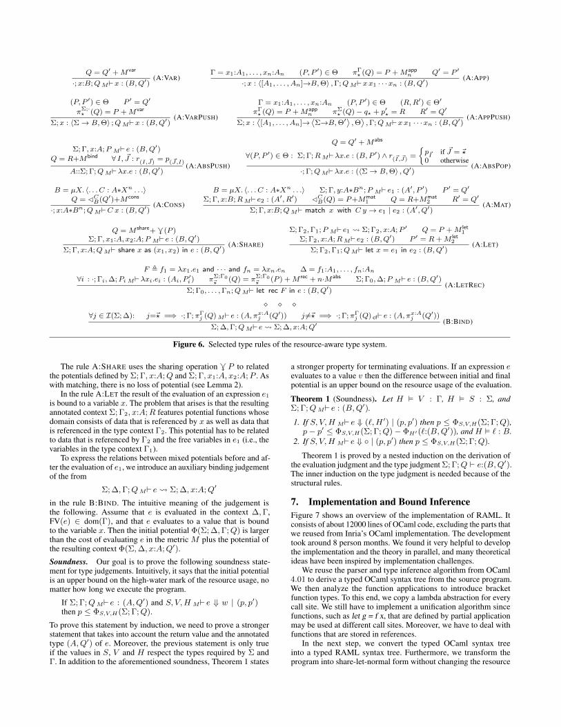
Type Rules. Figure 6 shows selected type rules for annotated types.All rules can be found in the TR.

The rule A:VAR can only be applied if the type stack Σ is empty.It then simply accounts for the cost M var and passes the potentialthat is assigned to the variable by the type context to the result type.If the type stack is not empty then the rule A:VARPUSH has tobe applied. In this case, the variable x must have a function type.We then look up a possible type annotation for the arguments andthe result (P, P ′) ∈ Θ in the type context, account for the cost ofvariable look-up (M var) and behave as specified by (P, P ′). We donot account for the cost of the “function application” because is costis handled in the rules A:APP and A:APPPUSH.

The rules A:APP and A:APPPUSH correspond to the simple typerules T:APP and T:APPPUSH. In A:APP we assume that the typestack is empty. We account for the cost M app

n of applying a functionto n arguments and look up valid potential annotations (P, P ′) forthe function body in the function annotation Θ. We then require thatwe have the potential specified by P available and return potentialas specified by P ′. In the rule A:APPPUSH we account for twoapplications: We first account for the function application as in therule A:APP. We then assume that the return type is a function typeand apply the arguments that are stored on the type stack Σ as wedo in the rule A:VARPUSH.

The rules A:ABSPUSH and A:ABSPOP for lambda abstractioncorrespond the rules T:ABSPUSH and T:ABSPOP. As in the simpletype system we can use them to non-deterministically pop the typestack Σ. When we do so in the rule A:ABSPOP, we create thefunction annotation Θ by essentially deriving Σ; Γ;P M`λx.e :(B,P ′) for every (P, P ′) ∈ Θ. However, we throw away allpotential that depends on the context Γ and only use the potentialthat is assigned the arguments Σ (annotation R).

The rule A:CONS assigns potential to a new node of an induc-tive data structure. The The C-unfolding CCB(Q′) transforms theannotation Q′ to an annotation Q for the context ·;x:A∗Bn. InA:MAT, the initial potential defined by the annotation Q of thecontext Σ; Γ, x:B has to be sufficient to pay the costs of the evalu-ation of e1 or e2 and the potential defined by the annotation Q′ ofthe result type. To type the expression e2 we basically just use theannotationQ. To type the expression e1, we rely on the C-unfoldingCCB(Q) that results in an annotation for the context Σ; Γ, y:A∗Bn.In both rules, there is no loss of potential (see Lemma 1).

Q = Q′ +Mvar

·;x:B;QM`x : (B,Q′)(A:VAR)

Γ = x1:A1, . . . , xn:An (P, P ′) ∈ Θ πΓ? (Q) = P +Mapp

n Q′ = P ′

·;x : 〈[A1, . . . , An]→B,Θ〉 ,Γ;QM`xx1 · · ·xn : (B,Q′)(A:APP)

(P, P ′) ∈ Θ P ′ = Q′

πΣ;·? (Q) = P +Mvar

Σ;x : 〈Σ→ B,Θ〉 ;QM`x : (B,Q′)(A:VARPUSH)

Γ = x1:A1, . . . , xn:An (P, P ′) ∈ Θ (R,R′) ∈ Θ′

πΓ? (Q) = P +Mapp

n πΣ? (Q)− q? + p′? = R R′ = Q′

Σ;x :⟨[A1, . . . , An]→

⟨Σ→B,Θ′

⟩,Θ⟩,Γ;QM`xx1 · · ·xn : (B,Q′)

(A:APPPUSH)

Σ; Γ, x:A;P M` e : (B,Q′)

Q = R+Mbind ∀ I, ~J : r(I, ~J)

= p(~J,I)

A::Σ; Γ;QM`λx.e : (B,Q′)(A:ABSPUSH)

Q = Q′ +Mabs

∀(P, P ′) ∈ Θ : Σ; Γ;RM`λx.e : (B,P ′) ∧ r(~I, ~J)

=

{p~I if ~J = ~?0 otherwise

·; Γ;QM`λx.e : (〈Σ→ B,Θ〉 , Q′)(A:ABSPOP)

B = µX. 〈. . . C : A∗Xn . . .〉Q = CCB(Q′)+M cons

·;x:A∗Bn;QM`C x : (B,Q′)(A:CONS)

B = µX. 〈. . . C : A∗Xn . . .〉 Σ; Γ, y:A∗Bn;P M` e1 : (A′, P ′) P ′ = Q′

Σ; Γ, x:B;RM` e2 : (A′, R′) CCB(Q) = P+Mmat1 Q = R+Mmat

2 R′ = Q′

Σ; Γ, x:B;QM` match x with C y → e1 | e2 : (A′, Q′)(A:MAT)

Q = M share+ .(P )Σ; Γ, x1:A, x2:A;P M` e : (B,Q′)

Σ; Γ, x:A;QM` share x as (x1, x2) in e : (B,Q′)(A:SHARE)

Σ; Γ2,Γ1;P M` e1 Σ; Γ2, x:A;P ′ Q = P +M let1

Σ; Γ2, x:A;RM` e2 : (B,Q′) P ′ = R+M let2

Σ; Γ2,Γ1;QM` let x = e1 in e2 : (B,Q′)(A:LET)

F , f1 = λx1.e1 and · · · and fn = λxn.en ∆ = f1:A1, . . . , fn:An∀i : ·; Γi,∆;Pi M`λxi.ei : (Ai, P

′i ) πΣ;Γ0

~?(Q) = πΣ;Γ0

~?(P ) +M rec + n·Mabs Σ; Γ0,∆;P M` e : (B,Q′)

Σ; Γ0, . . . ,Γn;QM` let rec F in e : (B,Q′)(A:LETREC)

� � �∀j ∈ I(Σ; ∆): j=~? =⇒ ·; Γ;πΓ

j (Q)M` e : (A, πx:Aj (Q′)) j 6=~? =⇒ ·; Γ;πΓ

j (Q) cf` e : (A, πx:Aj (Q′))

Σ; ∆,Γ;QM` e Σ; ∆, x:A;Q′(B:BIND)

Figure 6. Selected type rules of the resource-aware type system.

The rule A:SHARE uses the sharing operation . P to relatedthe potentials defined by Σ; Γ, x:A;Q and Σ; Γ, x1:A, x2:A;P . Aswith matching, there is no loss of potential (see Lemma 2).

In the rule A:LET the result of the evaluation of an expression e1

is bound to a variable x. The problem that arises is that the resultingannotated context Σ; Γ2, x:A;R features potential functions whosedomain consists of data that is referenced by x as well as data thatis referenced in the type context Γ2. This potential has to be relatedto data that is referenced by Γ2 and the free variables in e1 (i.e., thevariables in the type context Γ1).

To express the relations between mixed potentials before and af-ter the evaluation of e1, we introduce an auxiliary binding judgementof the from

Σ; ∆,Γ;QM` e Σ; ∆, x:A;Q′

in the rule B:BIND. The intuitive meaning of the judgement isthe following. Assume that e is evaluated in the context ∆,Γ,FV(e) ∈ dom(Γ), and that e evaluates to a value that is boundto the variable x. Then the initial potential Φ(Σ; ∆,Γ;Q) is largerthan the cost of evaluating e in the metric M plus the potential ofthe resulting context Φ(Σ,∆, x:A;Q′).

Soundness. Our goal is to prove the following soundness state-ment for type judgements. Intuitively, it says that the initial potentialis an upper bound on the high-water mark of the resource usage, nomatter how long we execute the program.

If Σ; Γ;QM` e : (A,Q′) and S, V,H M` e ⇓ w | (p, p′)then p ≤ ΦS,V,H(Σ; Γ;Q).

To prove this statement by induction, we need to prove a strongerstatement that takes into account the return value and the annotatedtype (A,Q′) of e. Moreover, the previous statement is only trueif the values in S, V and H respect the types required by Σ andΓ. In addition to the aforementioned soundness, Theorem 1 states

a stronger property for terminating evaluations. If an expression eevaluates to a value v then the difference between initial and finalpotential is an upper bound on the resource usage of the evaluation.

Theorem 1 (Soundness). Let H � V : Γ, H � S : Σ, andΣ; Γ;QM` e : (B,Q′).

1. If S, V,H M` e ⇓ (`,H ′) | (p, p′) then p ≤ ΦS,V,H(Σ; Γ;Q),p− p′ ≤ ΦS,V,H(Σ; Γ;Q)− ΦH′(`:(B,Q′)), and H � ` : B.

2. If S, V,H M` e ⇓ ◦ | (p, p′) then p ≤ ΦS,V,H(Σ; Γ;Q).

Theorem 1 is proved by a nested induction on the derivation ofthe evaluation judgment and the type judgment Σ; Γ;Q ` e:(B,Q′).The inner induction on the type judgment is needed because of thestructural rules.

7. Implementation and Bound InferenceFigure 7 shows an overview of the implementation of RAML. Itconsists of about 12000 lines of OCaml code, excluding the parts thatwe reused from Inria’s OCaml implementation. The developmenttook around 8 person months. We found it very helpful to developthe implementation and the theory in parallel, and many theoreticalideas have been inspired by implementation challenges.

We reuse the parser and type inference algorithm from OCaml4.01 to derive a typed OCaml syntax tree from the source program.We then analyze the function applications to introduce bracketfunction types. To this end, we copy a lambda abstraction for everycall site. We still have to implement a unification algorithm sincefunctions, such as let g = f x, that are defined by partial applicationmay be used at different call sites. Moreover, we have to deal withfunctions that are stored in references.

In the next step, we convert the typed OCaml syntax treeinto a typed RAML syntax tree. Furthermore, we transform theprogram into share-let-normal form without changing the resource

Parser

Type Inference

Source Code

Typed OCamlSyntax Tree

OCamlBytecode

RAML Compiler

Bracket-Type Inference

Stack-Based Type Checking

Explicit Let Polymorphism

Typed RAML Syntax Tree

OCaml-C Bindings

RAML Analyzer

Resource Type Interpretation

LP Solver Frontend

Multivariate AARA

CLP

Resource Metrics

Resource Bounds

Share-Let Normal Form

Figure 7. Implementation of RAML.

behavior. For this purpose, each syntactic form has a free flagthat specifies whether it contributes to the cost of the originalprogram. For example, all share expressions that are introduced inthe transformation are free. We also insert eta expansions wheneverthey do not influence resource usage.

After this compilation phase, we perform the actual multivariateAARA on the program in share-let-normal form. Resource metricscan be easily specified by a user. We include a metric for heapcells, evaluation steps, and ticks. Ticks allows the user to flexiblyspecify the resource cost of programs by inserting tick commandsRaml.tick(q) where q is a (possibly negative) floating-point number.In principle, the bound inference works similarly as in previousAARA systems [31, 34]: First, we fix a maximal degree of thebounds and annotate all types in the derivation of the simple typeswith variables that correspond to type annotations for resourcepolynomials of that degree. Second, we generate a set of linearinequalities, which express the relationships between the addedannotation variables as specified by the type rules. Third, wesolve the inequalities with Coin-Or’s LP solver CLP. A solutionof the linear program corresponds to a type derivation in whichthe variables in the type annotations are instantiated accordingto the solution. The objective function contains the coefficientsof the resource annotation of the program inputs to minimize theinitial potential. Modern LP solvers provide support for iterativesolving that allows us to prioritize minimization of higher-degreeannotations.

The type system we use in the implementation significantlydiffers from the declarative version we describe in this article. Forone thing, we have to use algorithmic versions of the type rules inthe inference in which the non-syntax-directed rules are integratedinto the syntax-directed ones [32]. For another thing, we annotatefunction types not with a set of type annotations but with a functionthat returns an annotation for the result type if presented with anannotation of the argument type. These annotations are symbolic andthe actual numbers are yet to be determined. So function annotationshave the side effect of sending constraints to the LP solver.

To make the resource analysis more expressive, we also allowresource-polymorphic recursion. This means that the type annotationin the recursive call differs from the annotations in the argumentand result types of the function. To infer such types we successivelyinfer type annotations of higher degree [30, 32].

Most of the generated constraints have the form of a so-callednetwork-flow problem [55]. LP solvers can handle network problemsvery efficiently and in practice CLP solves the constraints RAMLgenerates in linear time.

Apart from the analysis itself, we also implemented the con-version of the derived resource polynomials into easily-understoodpolynomial bounds and a pretty printer for RAML types and expres-sions. Additionally, we implemented an efficient RAML interpreterthat we use for debugging and to determine the quality of the bounds.

8. Experimental EvaluationThe development of RAML has been driven by an ongoing experi-mental evaluation with OCaml code. Our goal has been to ensure

let comp f x g = fun z → f x (g z)

let rec walk f xs =match xs with | [] → (fun z → z)| x::ys → match x with

| Left _ →fun y → comp (walk f) ys (fun z → x::z) y

| Right l →let x’ = Right (quicksort f l) infun y → comp (walk f) ys (fun z → x’::z) y

let rev_sort f l = walk f l []

RAML output for rev_sort (0.68s run time; steps metric):

10 + 23*K’ + 32*L’ + 20*L’*Y + 13*L’*Y^2

Figure 8. Modified challenge example from Avanzini et al. [10]and shortened output of the automatic bound analysis. We assume0 cost of the higher-order argument f. The derived bound on thenumber of steps is tight. L′ is the number of Right-nodes in theinput list,K′ is the number Left-nodes, and Y is the maximal lengthof the lists in the Right-nodes.

that the derived bounds are precise, that different programmingstyles are supported, that the analysis is efficient, and that existingcode can be analyzed. During the evaluation, we applied our auto-matic resource bound analysis to 411 functions and 6018 lines ofcode. The experiments have been performed with a 2.6 GHz IntelCore i5 MacBook Pro with 16GB RAM. The source code of RAMLas well as all OCaml files used in the experiments are availableonline [28]. The website also provides an easy-to-use web interfacethat can be used to experiment with RAML.

Analyzed Code and Limitations. The experiments have been per-formed with code from four sources: extracted OCaml code fromCoq specifications in CompCert [47], code from an OCaml tuto-rial [49], the OCaml standard library, and code written by us. Forthe handwritten code, we mostly implemented classical textbookalgorithms and use cases inspired from real-word applications. Thetextbook algorithms include algorithms for matrices, graph algo-rithms, search algorithms, and classic examples from amortizedanalysis such as functional queues and binary counters. The usecases include energy management in an autonomous mobile deviceand calling Amazon’s Dynamo DB from OCaml (see Section 9).

OCaml is a complex programming language and RAML doesnot yet support all language features of OCaml. This includesmodules, object-oriented features, record types, built-in equality,strings, nested patterns, and calls to native C functions. If RAMLcan be applied to existing code then the results are often satisfactory.For instance, we applied RAML to OCaml’s standard list librarylist.ml: In 3.2 seconds RAML automatically derives evaluation-stepbounds for 47 of the 51 top-level functions. All derived bounds areasymptotically tight. The 4 functions that cannot be bounded byRAML all rely on functions whose termination (and thus resourceusage) depends on an arithmetic integer operations, which arecurrently unsupported. The file list.ml consists of 428 LOC.

RAML fails if the resource usage can only be bounded by ameasure that depends on a semantic property of the program ora measure that depends on the difference of the sizes of two datastructures. Loose bounds are often the result of inter-proceduraldependencies. For instance, the worst-case behaviors of two func-tions f and g might be triggered by different inputs. However, theanalysis would add up the worst-case behaviors of both functions ina program such as f(a);g(a). Another reason for loose bounds is thata tight bound cannot be represented by our resource polynomials.

Example Experiment. To give an impression of the experimentswe performed, Figure 8 contains the output of an analysis of achallenging function in RAML. The code is an adoption of anexample that has been recently presented by Avanzini et al. [10] asa function that can not be handled by existing tools. To illustrate thechallenges of resource analysis for higher-order programs, Avanziniet al. implemented a (somewhat contrived) reverse function rev forlists using higher-order functions. RAML automatically derives atight linear bound on the number of steps used by rev.

To use more features of our analysis, we modified Avanziniet al.’s rev in Figure 8 by adding an additional argument f and apattern match to the definition of the function walk. The resultingtype of walk is α → α → bool) → [(β ∗ α list) either list; (β ∗α list) either list]→ (β∗α list) either list . Like before the modifica-tion, walk is essentially the rev_append function for lists. However,we assume that the input lists contain nodes of the form Left a orRight b so that b is a list. During the reverse process of the firstlist in the argument, we sort each list that is contained in a Right-node using the standard implementation of quick sort (not givenhere). RAML derives the tight evaluation-step bound that is shownin Figure 8. Since the comparison function for quicksort (argumentf) is not available, RAML assumes that it does not consume anyresources. If rev_sort is applied to a concrete argument f then theanalysis is repeated to derive a bound for this instance.

CompCert Evaluation. We also performed an evaluation with theOCaml code that is created by Coq’s code extraction mechanismduring the compilation of the verified CompCert compilers [47]. Wesorted the files topologically from their dependency requirements,and analyzed 13 files from the top. We could not process the filesfurther down the dependency graph because they heavily relied onmodules which we do not currently support. Using the evaluation-step metric, we analyzed 164 functions, 2740 LOC in 1300 seconds.

Figure 9 shows example functions from the CompCert codebase. As an artifact from the Coq code extraction, CompCert usestwo implementations of the reverse function for lists. The functionrev is a naive quadratic implementation that uses append and thefunction rev’ is an efficient tail-recursive linear implementation.RAML automatically derives precise evaluation step bounds forboth functions. As a result, a Coq user who is inspecting the derivedbounds for the extracted OCaml code is likely to spot performanceproblems resulting from the use of rev.

Summary of Results. Table 1 contains a compilation of the ex-perimental results. The first 3 rows show the results for OCamllibraries, handwritten code, and the OCaml tutorial [49]. The lastrow shows the results for CompCert [47]. The column LOC containsthe total number of lines of OCaml code that has been analyzed withthe respective metric. Similarly, the column Time contains the totaltime of all analyses with this metric. The column #Poly containsthe number of functions for which RAML automatically derived abound. The columns #Const, #Lin, #Quad, and #Cubic show thenumber of derived bounds that are constant, linear, quadratic, andcubic. Finally, columns #Failed and Asym.Tight contain the numberof examples for which RAML is unable to derive a bound and thenumber of bounds that are asymptotically tight, respectively. Wealso experimented with example inputs to determine the precisionof the constant factors in the bounds. In general, the bounds are veryprecise and often match the actual worse-case behavior.

The reported numbers result from the analysis of 411 non-trivialfunctions that are (with a few exceptions) recursive and higher order.The TR contains a short description of every function that is part ofthe evaluation, along with its type, the run time of the analysis, andthe derived bounds. The functions have been automatically analyzedusing the steps metric that counts the number of evaluation stepsand the heap metric that counts the number of allocated heap cells.

let rec app l m = match l with | [] → m| a :: l1 → a :: (app l1 m)

let rec rev = function | [] → []| x :: l’ → app (rev l’) (x :: [])

let rec rev_append l l’ = match l with | [] → l’| a :: l0 → rev_append l0 (a :: l’)

let rev’ l = rev_append l []

RAML output for rev (0.1s run time; steps metric):3 + 9.5*M + 4.5*M^2

RAML output for rev’ (0.05s run time; steps metric):7 + 9*M

Figure 9. Two implementations of list reverse that are used in theCompCert C compiler [47]; one is linear and the other is quadratic.

Moreover, we have used the tick metric to add custom cost measuresto some of the functions. These measures vary from program toprogram and include number of function calls, energy consumption,and amount of data sent to the cloud. Details can be found in thesource code [28].

There are two main reasons for the difference between theruntime of the analysis per function for the CompCert code (7.9s)and the other evaluated code (0.29s). First, the CompCert codecontains more complex data structures and we thus track morecoefficients. Second, there is a larger percentage of functions forwhich we cannot derive a bound (15.8% vs. 1.6%). As a result,RAML looks for bounds of higher degree before giving up. Bothleads to a larger number of constraints to solve for the LP solver.Finally, there are a few outlier functions that cause an unusuallylong analysis time. This is possibly due to a performance bug.

In general, the analysis is efficient in practice. However, RAMLis slowing down if the analyzed program contains many variables orfunctions with many arguments. Another source of complexity is themaximal degree of polynomials in the search space. Depending onthe complexity of the program, the analysis becomes unusable whensearching for bounds with maximal degree 7 − 9. The efficiencycould be improved by combining amortized resource analysis withdata-flow analyses and heuristics that predict the parts of the inputthat cause higher-degree resource usage.

9. Case Study: Bounds for DynamoDB QueriesHaving integrated the analysis with Inria’s OCaml compiler enablesus to analyze and compile real programs. An interesting use caseof our resource bound analysis is to infer worst-case bounds onDynamoDB queries. DynamoDB is a commercial NoSQL clouddatabase service, which is part of Amazon Web Services (AWS).Amazon charges DynamoDB users on a combination of numberof queries, transmitted fields, and throughput. Since DynamoDBis a NoSQL service, it is often only possible to retrieve the wholetable—which can be expensive for large data sets—or single entriesthat are identified by a key value. The DynamoDB API is availablethrough the Opam package aws. We make the API available to theanalysis by using tick functions that specify resource usage. Sincethe query cost for different tables can be different, we provide onefunction per action and table.

let db_query student_id course_id =Raml.tick(1.0); Awslib.get_item ...

In the following, we describe the analysis of a specific OCamlapplication that uses a database that contains a large table that stores

Metric #Funs LOC Time #Const #Lin #Quad #Cubic #Poly #Failed Asym.Tightsteps 243 3218 72.10s 16 130 60 28 239 4 225heap 243 3218 70.36s 41 112 60 22 239 4 225

tick 174 2144 64.68s 19 79 53 19 174 0 160CompCert steps 164 2740 1300.91s 32 99 7 0 138 26 137

Table 1. Overview of experimental results.

grades of students for different courses. Our first function computesthe average grade of a student for a given list of courses.

let avge_grade student_id course_ids =let f acc cid =

let (length,sum) = acc inlet grade = match db_query student_id cid with

| Some q → q| None → raise (Not_found (student_id,cid))

in (length +. 1.0, sum +. grade)inlet (length,sum) = foldl f (0.0,0.0) course_ids insum /. length

In 0.03s RAML computes the tight bound 1 · m where m is thelength of the argument course_ids. We omit the standard definitionsof functions like foldl and map. However, they are not built-in intoour systems but the bounds are derived form first principles.

Next, we sort a given list of students based on the average gradesin a given list of classes using quick sort. As a first approximationwe use a comparison function that is based on average_grade.

let geq sid1 sid2 cour_ids =avge_grade sid1 cour_ids >= avge_grade sid2 cour_ids

This results in O(n2m) database queries where n is the number ofstudents andm is the number of courses. The reason is that there areO(n2) comparisons during a run of quick sort. Since the resourceusage of quick sort depends on the number of courses, we have tomake the list of courses an explicit argument and cannot store it inthe closure of the comparison function.

let rec partition gt acc l =match l with

| [] → let (cs,bs,_) = acc in (cs,bs)| x::xs → let (cs,bs,aux) = acc in

let acc’ = if gt x aux then (cs,x::bs,aux)else (x::cs,bs,aux)

in partition gt acc’ xs

let rec qsort gt aux l = match l with | [] → []| x::xs →

let ys,zs = partition (gt x) ([],[],aux) xs inappend (qsort gt aux ys) (x::(qsort gt aux zs))

let sort_students s_ids c_ids = qsort geq c_ids s_ids

In 0.31s RAML computes the tight bound n2m − nm forsort_students where n is the length of the argument s_ids andm is the length of the argument c_ids. The negative factor arisesfrom the translation of the resource polynomials to the standardbasis.

Given the alarming cubic bound, we reimplement our sortingfunction using memoization. To this end we create a table thatlooks up and stores for each student and course the grade inthe DynamoDB. We then replace the function db_query with thefunction lookup.

let lookup sid cid table =let cid_map = find (fun id → id = sid) table infind (fun id → id = cid) cid_map

For the resulting sorting function, RAML computes the tight boundnm in 0.87s.

10. Related WorkOur work builds on past research on automatic amortized resourceanalysis (AARA). AARA has been introduced by Hofmann andJost for a strict first-order functional language with built-in datatypes [34]. The technique has been applied to higher-order func-tional programs and user defined types [41], to derive stack-spacebounds [16], to programs with lazy evaluation [52, 58], to object-oriented programs [35, 38], to imperative integer programs [17] andto heap-manipulating programs by integrating it with separationlogic [8]. All the aforementioned amortized-analysis–based systemsare limited to linear bounds. Hoffmann et al. [29, 31, 32] presenteda multivariate AARA for a first-order language with built-in listsand binary trees. Hofmann and Moser [37] have proposed a gener-alization of this system in the context of (first-order) term rewritesystems. However, it is unclear how to automate this system. In thisarticle, we introduce the first AARA that is able to automaticallyderive (multivariate) polynomial bounds that depend on user-definedinductive data structures. Our system is the only one that can de-rive polynomial bounds for higher-order functions. Even for linearbounds, our analysis is more expressive than existing systems forstrict languages [41]. For instance, we can for the first time derivean evaluation-step bound for the curried append function for lists.Moreover, we integrated AARA for the first time with an existingindustrial-strength compiler.

Type systems for inferring and verifying resource bounds havebeen extensively studied. Vasconcelos et al. [56, 57] described anautomatic analysis system that is based on sized-types [39] andderives linear bounds for higher-order functional programs. Herewe derive polynomial bounds.

Dal Lago et al. [43, 44] introduced linear dependent types toobtain a complete analysis system for the time complexity of the call-by-name and call-by-value lambda calculus. Crary and Weirich [20]presented a type system for specifying and certifying resourceconsumption. Danielsson [22] developed a library for complexityanalyses of lazy functional programs that is based on dependenttypes and manual cost annotations. The advantage of our techniqueis that it is fully automatic.

Classically, cost analyses are often based on deriving and solvingrecurrence relations. This approach was pioneered by Wegbreit [59]and is actively studied for imperative languages [1, 5, 7, 25]. Theseworks are not concerned with higher-order functions and boundsdo not depend on user-defined data structures. Benzinger [11] hasapplied Wegbreit’s method in an automatic complexity analysisfor Nuprl terms. However, complexity information for higher-orderfunctions has to be provided explicitly. Grobauer [26] reported amechanism to automatically derive cost recurrences from DMLprograms using dependent types. Danner et al. [23, 24] propose atechnique to derive higher-order recurrence relations from higher-order programs. Solving the recurrences is not discussed in theseworks and in contrast to our work they are not able to automaticallyinfer closed-form bounds.

In an active area of research, techniques from term rewritingare applied to complexity analysis [9, 15, 50]; sometimes in combi-nation with amortized analysis [36]. These techniques are usuallyrestricted to first-order programs and time complexity. Avanzini etal. [10] proposed a complexity preserving defunctionalization to

deal with higher-order programs. While the transformation is asymp-totically complexity preserving, it is unclear whether this techniquecan derive bounds with precise constant factors. The implementationof the defunctionalization is combined with an existing first-orderbound analysis based on term rewriting. In contrast to RAML, theresulting analysis tool can derive bounds for functions whose costdepends on the sizes of data captured in closures. Advantages ofRAML include more precise (non-asymptotic) bounds, amortizedanalysis, and efficient bound inference using LP solving.

Abstract interpretation based approaches to resource analysis [12,18, 27, 53, 60] focus on first-order integer programs with loops.Çiçek et al. [19] study a type system for incremental complexity. Asimilar approach can be used to reason about the difference of theresource usage of two programs [61]. An advantage of our approachis that it is automatic.

Finally, there exists research that studies cost models to formallyanalyze parallel programs. Blelloch and Greiner [13] pioneeredthe cost measures work and depth. There are more advanced costmodels that take into account caches and IO (see, e.g., Blelloch andHarper [14]), However, these works do not provide machine supportfor deriving static cost bounds.

11. ConclusionWe have presented important steps towards a practical automaticresource bound analysis for OCaml. Our three main contributionsare (1) a novel automatic resource analysis system that infers multi-variate polynomial bounds that depend on size parameters of user-defined data structures, (2) the first AARA that infers polynomialbounds for higher-order functions, and (3) the integration of AARAwith the OCaml compiler.

As the title of this article indicates, there are many open problemsleft on the way to a resource analysis system for OCaml that can beused in every-day development. In the future, we plan to improvethe bound analysis for programs with side effects and exceptionsby adding potential to exceptions and mutable heap cells. We willalso work on mechanisms that allow user interaction for manuallyderiving bounds if the automation fails. Another future researchtopic is modules and generating efficient function summaries. Weare also working on generalization of our resource polynomials toenable the inference of non-polynomial bounds and bounds thatdepend on records, heights of data structures, and integers [17].

To make the system more practical, we will work on taking intoaccount garbage collection and the runtime system when derivingtime and space bounds. Finally, we will investigate techniques tolink the high-level bounds with hardware and the low-level codethat is produced by the compiler. These open questions are certainlychallenging but we are now in a good position to further push theboundaries of resource bound analysis.

AcknowledgmentsWe thank Zhong Shao, Quentin Carbonneaux, and the members ofthe PoP Group at Carnegie Mellon for discussions, comments, andsuggestions that improved this article and RAML. A special thanksgoes to Martin Hofmann, whose suggestion to integrate RAML withOCaml at POPL’14 in San Diego started this work. Finally, we thankthe anonymous reviewers for their helpful feedback.

This article is based on research that has been supported, in part,by AFRL under DARPA STAC award FA8750-15-C-0082, by NSFunder grant 1319671 (VeriQ), and by a Google Research Award.Any opinions, findings, and conclusions contained in this documentare those of the authors and do not necessarily reflect the views ofthe sponsoring organizations.

References[1] E. Albert, P. Arenas, S. Genaim, G. Puebla, and D. Zanardini. Cost

Analysis of Java Bytecode. In 16th European Symposium on Program-ming (ESOP’07), pages 157–172, 2007.

[2] E. Albert, P. Arenas, S. Genaim, and G. Puebla. Closed-Form UpperBounds in Static Cost Analysis. Journal of Automated Reasoning,pages 161–203, 2011.

[3] E. Albert, P. Arenas, S. Genaim, M. Gómez-Zamalloa, and G. Puebla.Automatic Inference of Resource Consumption Bounds. In Logic forProgramming, Artificial Intelligence, and Reasoning, 18th Conference(LPAR’12), pages 1–11, 2012.

[4] E. Albert, P. Arenas, S. Genaim, G. Puebla, and D. Zanardini. CostAnalysis of Object-Oriented Bytecode Programs. Theoretical ComputerScience, 413(1):142 – 159, 2012.

[5] E. Albert, J. C. Fernández, and G. Román-Díez. Non-cumulativeResource Analysis. In Tools and Algorithms for the Construction andAnalysis of Systems - 21st International Conference, (TACAS’15), pages85–100, 2015.

[6] C. Alias, A. Darte, P. Feautrier, and L. Gonnord. Multi-dimensionalRankings, Program Termination, and Complexity Bounds of FlowchartPrograms. In 17th International Static Analysis Symposium (SAS’10),pages 117–133, 2010.

[7] D. E. Alonso-Blas and S. Genaim. On the limits of the classicalapproach to cost analysis. In 19th International Static AnalysisSymposium (SAS’12), pages 405–421, 2012.

[8] R. Atkey. Amortised Resource Analysis with Separation Logic. In19th European Symposium on Programming (ESOP’10), pages 85–103,2010.

[9] M. Avanzini and G. Moser. A Combination Framework for Complex-ity. In 24th International Conference on Rewriting Techniques andApplications (RTA’13), pages 55–70, 2013.

[10] M. Avanzini, U. D. Lago, and G. Moser. Analysing the Complexityof Functional Programs: Higher-Order Meets First-Order. In 29thInternational Conference on Functional Programming (ICFP’15),pages 152–164, 2012.

[11] R. Benzinger. Automated Higher-Order Complexity Analysis. Theoret-ical Computer Science, 318(1-2):79–103, 2004.

[12] R. Blanc, T. A. Henzinger, T. Hottelier, and L. Kovács. ABC: AlgebraicBound Computation for Loops. In Logic for Programming, ArtificialIntelligence, and Reasoning - 16th International Conference (LPAR’10),pages 103–118, 2010.

[13] G. E. Blelloch and J. Greiner. A Provable Time and Space EfficientImplementation of NESL. In First International Conference onFunctional Programming (ICFP’96), pages 213–225, 1996.

[14] G. E. Blelloch and R. Harper. Cache and I/O Efficent Functional Algo-rithms. In 40th Symposium on Principles of Programming Languages(POPL’13), pages 39–50, 2013.

[15] M. Brockschmidt, F. Emmes, S. Falke, C. Fuhs, and J. Giesl. Alternat-ing Runtime and Size Complexity Analysis of Integer Programs. InTools and Algorithms for the Construction and Analysis of Systems:20th International Conference (TACAS’14), pages 140–155, 2014.

[16] B. Campbell. Amortised Memory Analysis using the Depth of DataStructures. In 18th European Symposium on Programming (ESOP’09),pages 190–204, 2009.

[17] Q. Carbonneaux, J. Hoffmann, and Z. Shao. Compositional CertifiedResource Bounds. In 36th Conference on Programming LanguageDesign and Implementation (PLDI’15), pages 467–478, 2015.

[18] P. Cerný, T. A. Henzinger, L. Kovács, A. Radhakrishna, and J. Zwirch-mayr. Segment Abstraction for Worst-Case Execution Time Analysis.In 24th European Symposium on Programming (ESOP’15), pages 105–131, 2015.

[19] E. Çiçek, D. Garg, and U. A. Acar. Refinement Types for IncrementalComputational Complexity. In 24th European Symposium on Program-ming (ESOP’15), pages 406–431, 2015.

[20] K. Crary and S. Weirich. Resource Bound Certification. In 27thSymposium on Principles of Programming Languages (POPL’00),pages 184–198, 2000.

[21] S. A. Crosby and D. S. Wallach. Denial of service via algorithmiccomplexity attacks. In 12th USENIX Security Symposium (USENIX’12),pages 3–3, 2003.

[22] N. A. Danielsson. Lightweight Semiformal Time Complexity Analysisfor Purely Functional Data Structures. In 35th Symposium on Principlesof Programming Languauges (POPL’08), pages 133–144, 2008.

[23] N. Danner, D. R. Licata, and R. Ramyaa. Denotational Cost Semanticsfor Functional Languages with Inductive Types. In 29th InternationalConference on Functional Programming (ICFP’15), pages 140–151,2012.

[24] N. Danner, J. Paykin, and J. S. Royer. A Static Cost Analysis for aHigher-Order Language. In 7th Workshop on Programming LanguagesMeets Program Verification (PLPV’13), pages 25–34, 2013.

[25] A. Flores-Montoya and R. Hähnle. Resource Analysis of ComplexPrograms with Cost Equations. In Programming Languages andSystems - 12th Asian Symposium (APLAS’14), pages 275–295, 2014.

[26] B. Grobauer. Cost Recurrences for DML Programs. In 6th InternationalConference on Functional Programming (ICFP’01), pages 253–264,2001.

[27] S. Gulwani, K. K. Mehra, and T. M. Chilimbi. SPEED: Precise and Effi-cient Static Estimation of Program Computational Complexity. In 36thSymposium on Principles of Programming Languauges (POPL’09),pages 127–139, 2009.

[28] J. Hoffmann. RAML Web Site. http://raml.co, 2016.[29] J. Hoffmann and M. Hofmann. Amortized Resource Analysis with

Polynomial Potential. In 19th European Symposium on Programming(ESOP’10), pages 287–306, 2010.

[30] J. Hoffmann and M. Hofmann. Amortized Resource Analysis withPolymorphic Recursion and Partial Big-Step Operational Semantics.In Programming Languages and Systems - 8th Asian Symposium(APLAS’10), pages 172–187, 2010.

[31] J. Hoffmann, K. Aehlig, and M. Hofmann. Multivariate AmortizedResource Analysis. In 38th Symposium on Principles of ProgrammingLanguages (POPL’11), pages 357–370, 2011.

[32] J. Hoffmann, K. Aehlig, and M. Hofmann. Multivariate AmortizedResource Analysis. ACM Transactions on Programming Languagesand Systems, 34:14:1–14:62, 2012.

[33] J. Hoffmann, A. Das, and S.-C. Weng. Towards Automatic ResourceBound Analysis for OCaml. ArXiv e-prints, 2016.

[34] M. Hofmann and S. Jost. Static Prediction of Heap Space Usage forFirst-Order Functional Programs. In 30th Symposium on Principles ofProgramming Languages (POPL’03), pages 185–197, 2003.

[35] M. Hofmann and S. Jost. Type-Based Amortised Heap-Space Analysis.In 15th European Symposium on Programming (ESOP’06), pages 22–37, 2006.

[36] M. Hofmann and G. Moser. Amortised Resource Analysis and TypedPolynomial Interpretations. In Rewriting and Typed Lambda Calculi(RTA-TLCA;14), pages 272–286, 2014.

[37] M. Hofmann and G. Moser. Multivariate Amortised Resource Analysisfor Term Rewrite Systems. In 13th International Conference on TypedLambda Calculi and Applications (TLCA’15), pages 241–256, 2015.

[38] M. Hofmann and D. Rodriguez. Automatic Type Inference for Amor-tised Heap-Space Analysis. In 22nd European Symposium on Program-ming (ESOP’13), pages 593–613, 2013.

[39] J. Hughes, L. Pareto, and A. Sabry. Proving the Correctness of ReactiveSystems Using Sized Types. In 23rd Symposium on Principles ofProgramming Languages (POPL’96), pages 410–423, 1996.

[40] G. Jin, L. Song, X. Shi, J. Scherpelz, and S. Lu. Understanding andDetecting Real-World Performance Bugs. In 33rd Conference onProgramming Language Design and Implementation PLDI’12, pages77–88, 2012.

[41] S. Jost, K. Hammond, H.-W. Loidl, and M. Hofmann. Static Determi-nation of Quantitative Resource Usage for Higher-Order Programs. In

37th Symposium on Principles of Programming Languages (POPL’10),pages 223–236, 2010.

[42] P. C. Kocher. Timing Attacks on Implementations of Diffie-Hellman,RSA, DSS, and Other Systems. In Advances in Cryptology - 16thAnnual International Cryptology Conference (CRYPTO’96), pages 104–113, 1996.

[43] U. D. Lago and M. Gaboardi. Linear Dependent Types and RelativeCompleteness. In 26th IEEE Symposium on Logic in Computer Science(LICS’11), pages 133–142, 2011.

[44] U. D. Lago and B. Petit. The Geometry of Types. In 40th Symposiumon Principles of Programming Languages (POPL’13), pages 167–178,2013.

[45] X. Leroy. The ZINC Experiment: An Economical Implementation ofthe ML Language. Technical report 117, INRIA, 1990.

[46] X. Leroy. From Krivine’s Machine to the Caml Implementation. http://pauillac.inria.fr/~xleroy/talks/zam-kazam05.pdf,2005. Invited talk, May 17, Workshop on the Krivine and ZINCAbstract Machines.

[47] X. Leroy. Formal Verification of a Realistic Compiler. Communicationsof the ACM, 52(7):107–115, 2009.

[48] X. Leroy, D. Doligez, A. Frisch, J. Garrigue, D. Rémy, and J. Vouillon.The OCaml system release 4.02. Technical report, Institut National deRecherche en Informatique et en Automatique, 2014.

[49] V. Nicollet. 99 problems (solved) in ocaml. https://ocaml.org/learn/tutorials/99problems.html, 2016.

[50] L. Noschinski, F. Emmes, and J. Giesl. Analyzing Innermost RuntimeComplexity of Term Rewriting by Dependency Pairs. Journal ofAutomated Reasoning, 51(1):27–56, 2013.

[51] O. Olivo, I. Dillig, and C. Lin. Static Detection of Asymptotic Per-formance Bugs in Collection Traversals. In Conference on Program-ming Language Design and Implementation (PLDI’15), pages 369–378,2015.

[52] H. R. Simões, P. B. Vasconcelos, M. Florido, S. Jost, and K. Hammond.Automatic Amortised Analysis of Dynamic Memory Allocation forLazy Functional Programs. In 17th International Conference onFunctional Programming (ICFP’12), pages 165–176, 2012.

[53] M. Sinn, F. Zuleger, and H. Veith. A Simple and Scalable Approachto Bound Analysis and Amortized Complexity Analysis. In ComputerAided Verification - 26th International Conference (CAV’14), page743–759, 2014.

[54] R. E. Tarjan. Amortized Computational Complexity. SIAM J. AlgebraicDiscrete Methods, 6(2):306–318, 1985.

[55] R. J. Vanderbei. Linear Programming: Foundations and Extensions.Springer US, 2001.

[56] P. Vasconcelos. Space Cost Analysis Using Sized Types. PhD thesis,School of Computer Science, University of St Andrews, 2008.

[57] P. B. Vasconcelos and K. Hammond. Inferring Costs for Recursive,Polymorphic and Higher-Order Functional Programs. In 15th In-ternational Conference on Implementation of Functional Languages(IFL’03), pages 86–101, 2003.

[58] P. B. Vasconcelos, S. Jost, M. Florido, and K. Hammond. Type-BasedAllocation Analysis for Co-recursion in Lazy Functional Languages.In 24th European Symposium on Programming (ESOP’15), pages 787–811, 2015.

[59] B. Wegbreit. Mechanical Program Analysis. Communications of theACM, 18(9):528–539, 1975.

[60] F. Zuleger, M. Sinn, S. Gulwani, and H. Veith. Bound Analysisof Imperative Programs with the Size-change Abstraction. In 18thInternational Static Analysis Symposium (SAS’11), pages 280–297,2011.

[61] E. Çiçek, G. Barthe, M. Gaboardi, D. Garg, and J. Hoffmann. RelationalCost Analysis. In 44th Symposium on Principles of ProgrammingLanguages (POPL’17), 2017. Forthcoming.