Workshop  Report

Towards achieving global closure of ocean heat and freshwater budgets: Recommendations for advancing research in air-sea fluxes through collaborative activities

Report of the CLIVAR/GSOP/WHOI Workshop

on Ocean Syntheses and Surface Flux Evaluation Woods Hole, Massachusetts, 27-30 November 2012

Lisan Yu, Keith Haines, Mark Bourassa, Meghan Cronin, Sergey Gulev, Simon Josey, Seiji Kato, Arun Kumar, Tony Lee, Dean Roemmich

May 2013

WCRP Informal/Series Report No. 13/2013 ICPO Informal Report 189/13

 

2    

CLIVAR is a component of the World Climate Research Programme (WCRP). WCRP is sponsored by the World Meterorological Organisation, the International Council for Science and the Intergovernmental Oceanographic Commission of UNESCO. The scientific planning and development of CLIVAR is under the guidance of the JSC Scientific Steering Group for CLIVAR assisted by the CLIVAR International Project Office. The Joint Scientific Committee (JSC) is the main body of WMO-ICSU-IOC formulating overall WCRP scientific concepts. Bibliographic Citation Lisan Yu, Keith Haines, Mark Bourassa, Meghan Cronin, Sergey Gulev, Simon Josey, Seiji Kato, Arun Kumar, Tony Lee, Dean Roemmich: Towards achieving global closure of ocean heat and freshwater budgets: Recommendations for advancing research in air-sea fluxes through collaborative activities. INTERNATIONAL CLIVAR PROJECT OFFICE, 2013: International CLIVAR Publication Series No 189. (not peer reviewed).

 

3    

The Organisers of the CLIVAR/GSOP/WHOI Workshop on Ocean Syntheses and Surface Flux Evaluation would like to thank the financial contribution provided by several agencies, whose support enabled the workshop to take place. Sponsor Agencies: NASA Physical Oceanography (Eric Lindstrom) NOAA Ocean Climate Observations (David Legler) US CLIVAR (Mike Patterson) WCRP/CLIVAR

 

4    

Table of Content 1. Workshop background and objectives 5

2. Workshop recommendations 12

2.1) Collaborative activities 13

2.1.1) Regional heat/salt budget analysis 13

2.1.2) Direct pointwise comparison with selected OceanSITES 15

2.2) Metrics for surface flux evaluation and improvements 19

2.2.1) Global 19

2.2.2) Regional 19

2.2.3) Local 19

2.2.4) Transport information from observations 19

2.3) Accuracy and resolution requirements 20

2.4) Data requirements and infrastructure to be enhanced 23

2.4.1) Mooring flux database 23

2.4.2) Research vessel flux database 23

2.5) Perspective of CAGE experiments 24

2.6) Argo’s current status and future enhancement plan 26

3. Summary of recommendations and future planning 27

Acknowledgements 29

References 30

Appendix A CLIVAR GSOP WHOI Workshop Agenda 35

Appendix B Author Affiliations 42

 

5    

1. Workshop background and objectives

The oceans have the largest heat capacity in the climate system and therefore control the rate of

climate change (Levitus et al. 2005; Lyman et al., 2010; Trenberth and Fasullo 2010; Loeb et al. 2012).

Ocean circulation redistributes heat and regulates air–sea fluxes, thus influencing climate variability

and change. The distribution and rate of change of ocean heat content is one of key observational

metrics for the IPCC and serves as a benchmark reference both for calibrating and evaluating climate

models such as CMIP5 and for the emerging decadal climate prediction effort (Hansen et al., 2005;

Meehl et al. 2011; Palmer et al. 2011). Improving the quantification of air–sea fluxes is identified as a

critical research area for advancing our understanding of atmosphere–ocean interactions related to

Earth’s climate variability and change, and for improving our ability to account for ocean signals in

short- and long-term climate fluctuations due to modes of natural variability and human influence.

Air–sea fluxes provide the fundamental links in virtually every atmosphere–ocean feedback

process. Any persistent changes to the energy balance will cause global and regional temperature

distributions to change, leading to changes in evaporation and precipitation that will then cause changes

in ocean salinity (and thus density). Both the atmosphere and oceans will respond with circulation

changes, if the air temperatures or ocean densities are altered, and with wind stress changes that lead to

further feedbacks on ocean circulation. There are many pathways by which regional energy and

freshwater budgets may be altered. Interactions between surface fluxes and atmospheric and ocean

transport variations are therefore complex and depend on the time scales of externally induced changes

(e.g., Bjerknes 1964; Shaffrey and Sutton 2006) driven by anthropogenic greenhouse gases, by

fluctuations in natural forcings (e.g., volcanic aerosols and solar output), and by internal variability of

the Earth’s coupled climate system (e.g., various modes of climate variability). Knowing how local

energy and freshwater budgets vary and contribute to both climate variability and change is deemed

 

6    

critically important toward evaluating the consequences of climate change on the energy and water

cycle (Trenberth et al., 2009).

Gridded air–sea flux products on basin and global scales are now produced by (i) atmospheric

reanalyses, (ii) ocean syntheses, and (iii) parameterized flux analyses using empirical bulk formulae

and available surface meteorological variables from satellite and ship observations and, in some

products, combined with atmospheric reanalyses (WCRP 1989; Fairall et al. 2010). One seemingly

unavoidable obstacle in air–sea flux estimation is the lack of sufficient direct flux measurements to

quantify the errors in the products and to assess climate-related signals with certainty. All flux products

suffer from uncertainties arising primarily from sampling issues, subgrid-scale parameterizations,

empirical estimates of parameters, and changes related to the observational systems (e.g., changes in

satellite sampling, aging of satellite sensors (e.g. Shie 2012)), transition from an in situ-dominated

observing system to a satellite-dominated observing system, etc). The errors involved in deriving these

products can accumulate and have major impacts on the accuracy of the flux products. This could lead

to, for example, large imbalances in the energy and freshwater budgets over the global oceans. The

uncertainties in existing gridded flux products preclude reliable estimates and assessment of the

sensitivity of air–sea exchange processes to long-term climate signals.

Air–sea variables and flux measurements by moored buoys and research vessels (Bradley and

Fairall 2007) are important benchmarks in evaluating basin- and global-scale parameterized flux

products (Josey and Smith 2006). However, they are available only at selected locations. These in situ

flux measurements alone are insufficient for addressing the imbalance problem in the global energy and

freshwater budget because of two limitations. The first is that in situ measurements are too limited in

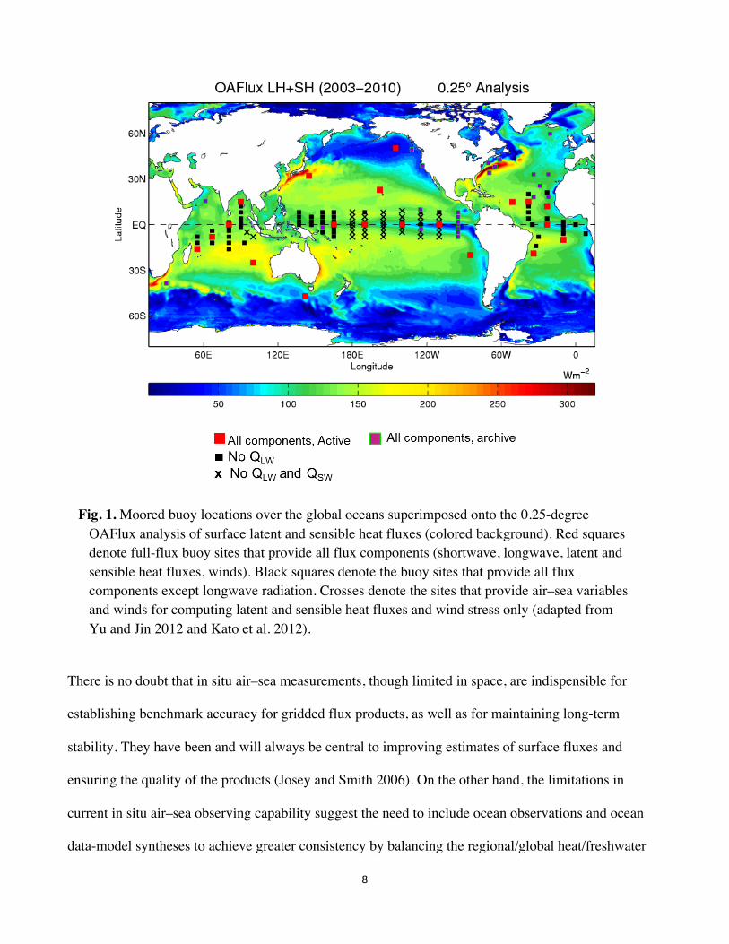
both spatial and temporal sampling. Figure 1 shows the locations of ~120 archived and active moored

buoys that provide measurements of partial or full-flux components useful for evaluating air–sea heat

fluxes. More than 85% of these buoys are located in the tropical oceans within 25 degrees north and

 

7    

south. The midlatitudes are covered by only a few long-term buoys, and the high latitudes have barely

any long-term stations. The geographic distribution of moored buoys is sparse and highly uneven,

which is particularly so for buoy longwave radiation measurements. There are currently only ~20

active buoys that are equipped with a pyrgeometer (longwave radiation sensor) over the global oceans.

Since the net air–sea heat flux is the sum of latent heat, sensible heat, and longwave and shortwave

radiation, this sets the limit for the number of full-flux buoy sites that can be used to validate global net

heat flux products. The ~20 “full-flux” sites are far from sufficient to quality-check the global accuracy

of the gridded products, let alone to address the imbalance problem in the global energy budget and the

freshwater budget. Even fewer buoys measure wave and current characteristics that are important for

accurate determination of turbulent fluxes.

The second limitation is that buoys do not have direct measurements of all flux components.

Buoy latent and sensible heat fluxes are computed from bulk flux algorithms, such as the COARE

algorithm by Fairall et al. (2003), using buoy measurements of air–sea variables (e.g., wind speed and

direction, near-surface air temperature/humidity, sea surface temperature, barometric pressure,

precipitation, incoming longwave and shortwave radiation). Since the same bulk flux algorithm is used

in constructing global gridded flux products, the buoy fluxes may not be completely independent of the

flux products being evaluated—although buoy air–sea observations are independent provided they are

not assimilated/synthesized. In recent years, direct measurements of latent heat, sensible heat, and

momentum flux components have been made possible by eddy-covariance methods (Edson et al.

1998), thus providing parallel sampling that helps to improve bulk flux algorithms. These direct and

indirect in situ flux time series datasets are both important benchmarks. When used together, they can

be beneficial to both algorithm improvement and flux product evaluation.

 

8    

Fig. 1. Moored buoy locations over the global oceans superimposed onto the 0.25-degree OAFlux analysis of surface latent and sensible heat fluxes (colored background). Red squares denote full-flux buoy sites that provide all flux components (shortwave, longwave, latent and sensible heat fluxes, winds). Black squares denote the buoy sites that provide all flux components except longwave radiation. Crosses denote the sites that provide air–sea variables and winds for computing latent and sensible heat fluxes and wind stress only (adapted from Yu and Jin 2012 and Kato et al. 2012).

There is no doubt that in situ air–sea measurements, though limited in space, are indispensible for

establishing benchmark accuracy for gridded flux products, as well as for maintaining long-term

stability. They have been and will always be central to improving estimates of surface fluxes and

ensuring the quality of the products (Josey and Smith 2006). On the other hand, the limitations in

current in situ air–sea observing capability suggest the need to include ocean observations and ocean

data-model syntheses to achieve greater consistency by balancing the regional/global heat/freshwater

 

9    

budgets. Studies by Wunsch and Heimbach (2009) and Douglass et al. (2010) are examples of the

applications of ocean observations and ocean synthesis to analyze regional and global heat and

freshwater budgets. The ENSO region is another example of where regional heat content is sufficient to

test models. Climate models have difficulty in correctly capturing air–sea fluxes of energy and

momentum, as demonstrated in an examination of El Nino–Southern Oscillation (ENSO)

characteristics found in the recent CMIP5 climate model comparison (Michael et al. 2013). In the

eastern tropical Pacific, thermocline depth is a proxy for heat content. Figure 2 shows that the CMIP5

model’s thermocline feedback (as described by the regression slope of SST anomalies to thermocline

depth anomalies) is too active in comparison with observations, which affect the air–sea fluxes

associated with ENSO. More work is required to provide observation-based fluxes for model

evaluation.

The Argo program over the past 10 years has grown into a near-global observing system for the

subsurface ocean with more than 3000 free-drifting, profiling floats monitoring the upper 2000 m of the

open oceans (Roemmich et al. 2009). The Argo subsurface temperature and salinity observations,

together with surface temperature and salinity observations from satellites (Lagerloef et al. 2008),

provide a new means to direct estimates of the total integrated air–sea fluxes of heat and freshwater

averaged on some spatial and temporal scales (Willis et al. 2004;

 

10    

Fig. 2. Comparison of two related ENSO characteristics as determined from ocean observations and the CMIP5 output. The ovals represent the best fit to anomalies in the eastern equatorial Pacific sea surface temperature (SSTa) and the thermocline depth as seen in observations (black ellipse) and 17 model runs (where only the first member of ensemble runs is examined). All the models have an exaggerated change in SST associated with changes in thermocline depth, suggesting that thermocline feedback associated with ENSO could be too strong, thus leading to errors in surface fluxes (from Michael et al. 2013)

von Schuckmann and Traon 2011). These ocean data potentially offer important regional references for

calibration of air–sea flux estimates in a way similar to flux buoy and ship measurements for pointwise

calibration information. However, they represent an integration, and they lack the sampling needed for

short-lived strong events that have large contributions to regional air–sea fluxes. Recent improvements

in satellite observations of stress, air temperature, and humidity are also expected to contribute to

improved accuracy of such exchanges.

 

11    

Air–sea fluxes represent an important crosscut area within WCRP that link the interests of

different core projects, including CLIVAR, GEWEX, and CLiC for the high-latitude areas including

sea ice zones. The twin challenges of constraining global ocean heat and freshwater budgets using both

models and observations, along with the importance of improving surface forcing functions for ocean

and coupled climate modeling purposes, highlight the need for close collaboration between the

observation (both in situ and remote sensing), modeling, and synthesis communities. The recent WCRP

action plan on Surface Fluxes published in January 2012, specifically states that “The evaluation of

model-based fluxes (NWP, atmospheric and ocean reanalysis) should be seen as an aspect of the

evaluation of global surface flux datasets, and handled through the establishment of specific task

groups.” In recognizing the challenges and opportunities ahead, the Global Synthesis and Observational

Panel (GSOP) of International CLIVAR worked closely with the air–sea flux and ocean synthesis

communities to organize a joint workshop to address the pressing challenges and needs through

collaboration. The workshop was held 27-30 November 2012, at the Woods Hole Oceanographic

Institution, Woods Hole, Massachusetts, and was sponsored jointly by NASA Physical Oceanography,

NOAA Ocean Climate Observations, US CLIVAR, and WCRP.

The workshop convened 60 researchers working on ocean observations, ocean syntheses, and

air–sea fluxes to (1) review achievements we have made collectively in recent decades in improving

air–sea flux observations and estimates; (2) discuss gaps and current limitations in global air–sea flux

products, with particular reference to constraining (even balancing) ocean heat and freshwater budgets;

(3) discuss challenges and advantages we have in planning our activities in the coming years; (4)

propose areas of collaboration with the ocean observation (in situ and satellite) community, the flux

modeling community, and the ocean data assimilation community that benefit air–sea flux activities;

and (5) develop recommendations and requirements for the areas of research that we could demonstrate

benefits through collaboration on both a 2-year and a 5-year timescale.

 

12    

NASA sponsor, Eric Lindstrom, put forth the following questions for the workshop attendees to

address and react to. (1) Reducing large uncertainties in air–sea flux products needs help from ocean

reanalysis. It seems that the advent of scatterometers, Argo, GHRSST, and Aquarius/SMOS should

have helped reduce uncertainty. Why hasn’t uncertainty been reduced more? (2) Is there a set of

principles and standards for generating flux products so that they all can be compared and contrasted

easily? (3) What is the best way to define “truth” against which flux products are judged? (4) What

are the key areas of research for which individual PI efforts or stove-piped efforts by individual

agencies fall short? What kind(s) of team effort can you imagine that CLIVAR could spearhead?

NOAA sponsor, David Legler, expanded the list with additional questions. What mechanisms are in

place and what evidence is there to indicate that flux fields are improving (e.g., uncertainties are better

characterized, and errors or error spread is reduced)? How do you know (or how do you not know)?

The 3.5-day meeting covered seven main themes, including (1) review of the present state of

air–sea flux estimation, (2) topical issues in air–sea flux estimation techniques, (3) topical issues in

regional air–sea flux estimation, (4) integrating air–sea fluxes with temperature and salinity

observations, (5) fluxes in coupled models and synthesis products, (6) synthesis evaluation and

intercomparison, and (7) synthesis applications and the way forward. The workshop evaluated flux

production activities and recommended flux-oriented comparisons based on essential ocean variable

metrics. These activities are highly relevant to the interests of the WOAP, WGSF, and the WCRP Data

Council. There were 58 oral/poster presentations. The workshop agenda, which contains the list of

presentations, is included in Appendix A.

2. Workshop recommendations

Given the gaps in present-day knowledge and understanding, a consensus was reached during

the workshop that achieving globally balanced energy and freshwater budgets is a long- term challenge,

 

13    

and should be broken down into incremental steps with achievable targets at each stage. Guided by the

NASA and NOAA perspectives and objectives, the workshop discussions were directed toward seeking

areas of collaborative research by maximizing the use of existing observations made at the ocean

surface and subsurface, and by integrating regional budget analysis with direct pointwise comparison

with in situ buoy/ship measurements. The following recommendations are developed and generalized

from the stimulating and productive discussion sessions during the workshop.

2.1) Collaborative activities

2.1.1) Regional heat/salt budget analysis

The advent of the complete Argo program is allowing upper ocean heat and salinity content to

be monitored both regionally and near globally (excluding polar areas and marginal seas). This

monitoring should be regarded as a means of providing direct estimates of the total integrated air–sea

fluxes of heat and freshwater averaged on some spatial and temporal scale, against which, in the future,

parameterized air–sea flux products may be calibrated. Rates of change in these integrated results can

be used to evaluate air–sea fluxes and local transport. These budgets, if estimates of uncertainty

included, can be examined for a wide variety of regions and on various time scales to provide insights

into the probability distribution of temporally averaged surface fluxes. Thus ocean data should be

capable of providing regional references for calibration of temporally integrated air–sea flux estimates

in the same way that flux buoy and ship measurements have previously provided pointwise calibration

information. Extending the calibration of air–sea flux products using regional scale constraints

provided by ocean data should greatly help to resolve the issues of regional biases and global

imbalance that currently affect almost all flux products constructed from satellites, ships, and

atmospheric reanalyses.

 

14    

However, there are several important caveats to achieving these goals. Regional ocean heat

budgets can provide information on the integrated heat flux but not the components, although the

regional freshwater budgets do provide a separate constraint on the latent heat flux through

evaporation. In addition, advective convergence and divergence of heat may be important in the

regional heat budgets, and if they cannot be sufficiently constrained these transport terms may

dominate the error estimate on the regional air–sea flux budgets.

Two solutions to this problem are proposed from the workshop.

a. Using ocean synthesis and reanalysis products, the advective convergence of heat and

freshwater can be constrained. In principle, the ocean transports ought to be well constrained

geostrophically by the assimilation of Argo and other in situ data. In practice, the synthesis

results have probably yet to attain the needed consistency in transports, and need to be properly

assessed.

b. Select budget study regions from which advective transports and their variability are likely to be

small to minimize the errors introduced into assessments of the surface fluxes.

A number of suggestions were made at the workshop to help in the selection of ocean regions

for flux budget studies. These included

a. Seek areas away from boundary currents where advective convergence is minimal. It is possible

that ocean synthesis or other modeling products could be used to assess the likely transports in

or out of such regions. Areas could include enclosed and semi-enclosed basins such as the

Mediterranean and the Red and Black seas.

b. Seek areas that include within them one or more flux buoys (e.g., the OceanSITES flux buoys or

an ongoing field program such as SPURS, particularly buoys associated with process study data

(e.g., STRATUS and PAPA) to allow for a direct regionalization and cross-referencing. It was

 

15    

also recommended that satellite data and other in situ data (ships and drifters) be used to

observe and/or assess the regional variability around the buoys.

c. Analyze areas of particular interest for ocean processes (e.g., other areas of water formation).

d. Choose areas with the best Argo sampling over the longest period.

These cross-reference studies would be a joint effort between the flux analysis, Argo, ocean

syntheses, and process study communities. It is recommended that a working group should be set

up to define regional flux budget areas that have good sampling of ocean properties and to define

the needed intercomparison studies. This activity would be closely allied to the development of a

buoy and research vessel flux database infrastructure where calibrated time series products could be

used for intercomparison with regional or global products on different time scales.

2.1.2) Direct pointwise comparison with selected OceanSITES

In situ air–sea flux measurements set the accuracy standard for gridded flux products. It is

recommended to proceed with regional heat/salt budget analyses in conjunction with direct

pointwise comparisons of different ocean synthesis products using air–sea buoy measurements at

selected full-flux sites (OceanSITES). Preliminary effort has been initiated for this workshop, and it is

recommended that these comparisons should be carried out for all global flux products, including

atmospheric reanalyses, ocean syntheses, and parameterized flux products. The analysis of the heat and

freshwater budgets from the different products around the calibration sites should yield insight into

synthesis product consistency, distributions and scaling effects, and areas of common biases, as well as

enable flux component comparisons. It is also suggested that these observations be compared to

satellite data for appropriate variables, with the goal of determining the importance of spatial and

 

16    

temporal variability (e.g., May and Bourassa 2011) in the unavoidable random errors associated with

comparison to the individual buoys.

There are ~20 full-flux buoy sites currently operating (Fig. 1). The OceanSITES buoys at the

following key climate locations are recommended.

a. The Tropical Oceans (20°S-20°N, 9 buoys)

The tropical moored buoy arrays of TAO, PIRATA, and RAMA

(http://www.pmel.noaa.gov/tao/oceansites/flux/main.html) deliver real-time measurements of

air–sea conditions for improved detection, description, understanding, and prediction of

regional climate variability on seasonal, intraseasonal, interannual, and longer time scales, that

include but are not limited to regional phenomena such as ENSO, monsoons, the Madden-Julian

oscillation, the Indian Ocean dipole, and tropical Atlantic variability. The selected buoys

include (i) two TAO buoys, one located in the eastern equatorial Pacific cold tongue at EQ,

110ºW and the other in the western equatorial Pacific warm pool at EQ, 165ºE; (ii) two RAMA

buoys, one in the central equatorial Indian Ocean at EQ, 80ºE, and the other in the Bay of

Bengal warm water pool at 15ºN, 90ºE; and (iii) three PIRATA buoys, one in the central

equatorial Atlantic at EQ, 23ºW, one in the tropical southwest Atlantic at 10ºS, 10ºW, and one

in the tropical northwest Atlantic at 15ºN, 38ºW.

In addition to the buoys from the tropical moored arrays, two OceanSITES buoys

deployed by WHOI Upper Ocean Process Group (http://uop.whoi.edu/) are selected to provide

vital air–sea measurements in regions that are not covered by the tropical arrays. The two

WHOI buoys are from (i) the STRATUS (20ºS, 85ºW) project that studies long-term evolution

and coupling of the boundary layers in the STRATUS deck regions of the eastern tropical

Pacific, and (ii) the Northwest Tropical Atlantic Station (NTAS) (15ºN, 51ºW), both of which

 

17    

are well suited for investigations of surface forcing and oceanographic response in a region of

strong SST anomalies and significant local air–sea interactions.

b. The subtropical region (20–40 degrees north and south, 6 buoys)

The subtropics are regions of relatively large latent heat flux due to strong evaporation, with

maximum latent heat loss occurring over the western boundary currents (WBC) and extensions

during fall and winter seasons. Six buoys in these regions can be used to evaluate the

performance of gridded flux products; three are located in the open oceans and three are in the

regime of the WBC. The three buoys in the open oceans are (i) the RAMA buoy in the Indian

Ocean southeast trade wind regime at 20ºS, 100ºE

(http://www.pmel.noaa.gov/tao/oceansites/flux/main.html), (ii) the WHOI Hawaii Ocean Time-

series Station (WHOTS) in the north Pacific at 22.5ºN, 158ºW (http://uop.whoi.edu/), and (iii)

the Salinity Processes in the Upper Ocean Regional Study (SPURS) buoy in the north Atlantic

deployed by WHOI at 24.5ºN, 38ºW (http://uop.whoi.edu/). The three WBC-related buoys are

(i) the Kuroshio Extension Observatory (KEO) buoy located in the recirculation gyre south of

the Kuroshio Extension at 144.6°E, 32.4°N (http://www.pmel.noaa.gov/keo/), (ii) the

JAMSTEC Kuroshio Extension Observatory (JKEO) in the north Kuroshio Extension region at

38ºN, 146.5ºE (http://www.jamstec.go.jp/iorgc/ocorp/ktsfg/data/jkeo/), and (iii) the CLIVAR

Mode Water Dynamic Experiment (CLIMODE) buoy deployed by WHOI in the core of the

mean Gulf Stream at 38.5ºN, 65ºW (http://uop.whoi.edu/).

c. Higher latitudes (poleward of 40 degrees north and south, 2 buoys)

Higher latitude surface fluxes differ markedly from those in temperate regions because of

changes of several key air–sea variables, such as strong seasonality, very low winter air

temperatures, frequent extreme weather events with high wind speeds, large local variability

associated with mesoscale eddies and ocean fronts, etc. Uncertainties in gridded flux products

 

18    

are large at higher latitudes and in situ validation datasets are sparse. Two reference stations are

recommended, including (i) Ocean Station PAPA (http://www.pmel.noaa.gov/stnP/index.html)

located at 50ºN, 145ºW to monitor air–sea interaction for the harsh conditions of the North

Pacific region, and (ii) the Southern Ocean Flux Station (SOFS; http://imos.org.au/SOTS.html)

located in the sub-Antarctic Zone near 47ºS, 140ºE, the site critical for studying air–sea

interaction that affects regional climate variability on a wide range of time scales. The site is

particularly vulnerable to the extreme weather events that typify the area, including very large

waves, strong currents, and severe storms.

It is recommended that, to obtain independent comparisons, reference station data

(identified by an “84” in its WMO number) be withheld from assimilation in reanalyses to

provide an independent verification of these products and their parameterization schemes.

Likewise, it is recommended that the WMO numbers of data that are assimilated into NWP be

listed and made available.

It is also recommended that, to facilitate the comparisons between different products,

ocean synthesis and reanalysis groups separately archive the components of the air–sea heat flux,

i.e., short and longwave radiation and sensible and latent heat fluxes, in addition to the other

variables needed for net budget studies. This is not commonly done and these components need to be

separately compared with observations to improve understanding of the flux exchange processes.

Importantly, the point comparisons should be supported with scaling analysis and estimation of

the uncertainties imposed by spatial/temporal variations in surface fluxes and flux-related variables

when point measurements are co-located with the gridded products or/and grid cell averages.

 

19    

2.2) Metrics for surface flux evaluation and improvements

A white paper on “Guidelines for Evaluation of Air-Sea Heat, Freshwater and Momentum Flux

Datasets” was developed previously under GSOP (Josey and Smith 2006). It provides a basis for flux

evaluation using global, regional, and local metrics as summarized below.

2.2.1) Global:

Metrics should include global mean Qnet and means for individual flux components along

with characteristics of the statistical distributions of surface fluxes presented as climate maps

and zonal means.

2.2.2) Regional:

Metrics should include the following two sets of computation.

a. Comparison of integrated net surface heat flux estimates for regions bound by reliable

oceanographic heat transport estimates with the corresponding heat transport implied value.

b. Integrated surface flux estimates of individual flux components for selected regions with

reasonably good coverage by in-situ observations and likely small impact of ocean dynamics

and lateral advection, heat and freshwater budgets of selected semi-enclosed seas (Red,

Mediterranean, Black, Baltic—with a caveat on the Gulf of Bothnia and the Great Lakes).

The time series of these statistics is also highly desirable. Care needs to be taken here as

conclusions reached for enclosed seas may not be valid for the open ocean.

2.2.3) Local:

Metrics should include time series analysis along with probability and spectral characteristics

of fluxes in the buoy and OWS locations.

2.2.4) Transport information from observations

It is important that relevant metrics should be combined wherever possible as this will help

avoid biases developing in surface flux products derived through parameterization over

 

20    

large scales, for which nonlinearities make parameter estimation problematic. Ocean

transports, whether determined traditionally from hydrographic sections, or monitored

continuously (e. g. as in the RAPID array (Cunningham et al 2007)), or using sections

adjusted by inverse modeling (e. g. Lumpkin and Speer 2007), or through transports

evaluated from ocean syntheses or reanalyses, can provide valuable constraints for

evaluating regional air-sea fluxes.

One of the drawbacks of using such data in the past has been the asynoptic sampling and

therefore the need to assume a steady state to infer surface flux information. However, the

RAPID array is providing continuous monitoring of flow across an entire ocean section, and

synthesis or reanalysis studies allow transports to be derived from asynoptic ocean

observations without assuming steady state conditions. A number of studies are currently

underway to use the RAPID data as a constraint on the heat budget changes in the North

Atlantic and similarly for the freshwater budgets. Although still in their early stages, results

are promising.

It is recommended that using ocean transport monitoring across key ocean sections

including RAPID would be of considerable benefit to the reduction in uncertainty of surface

fluxes and would contribute to proper closure of regional budgets, which are of great importance

for understanding regional climate change.

2.3) Accuracy and resolution requirements

The accuracy goals for net surface heat flux measurement were set at ±10 Wm-2 on annual time

scales during the WOCE observing program (WCRP 1989) and the TOGA-COARE process study

(Webster and Lukas 1992; Weller et al. 2004). However, accuracy and resolution requirements for air–

sea fluxes are highly dependent on the spatial and temporal scales of the specific process studied. The

 

21    

need for imposing an accuracy standard that is better than 10Wm-2 has been articulated by many

applications. Figure 3 summarizes the accuracies for net heat flux and surface winds desired by

applications to key processes in meteorology, oceanography, and climate. In particular, the flux

products would be required to be as accurate as 0.1Wm-2 (averaged over large space and time scales)

when used for detecting long-term climate change signals.

Fig. 3. A first-order estimation of flux and wind accuracies desired for various applications (Adapted from Bourassa et al. 2013). Fluxes expressed in W m-2 refer to total heat fluxes (including radiative and turbulent processes). Wind speeds expressed in ms-1 refer to surface winds. On short time scales, inaccuracies are usually dominated by random errors. On long time scales, the averaging is so great that random errors are small compared to biases.

At present, the global imbalance in the gridded products ranges between 2 Wm-2 and 30 Wm-2,

which is far from meeting the accuracy requirements for many applications. One difficulty is the lack

 

22    

of precision in knowing the net downward flux of energy associated with global warming, although we

know this cannot be large, likely no more than a few tenths of 1 Wm-2 on decadal time scales as

indicated from ocean temperature observations. Even atmospheric reanalyses and ocean syntheses each

use fixed surface boundary conditions and therefore lack consistent feedbacks that would allow air-sea

fluxes to be properly constrained against local observations. The newly developing field of coupled

data assimilation and coupled reanalysis should start to overcome this problem in future, but the

parameterized flux products which will be available for comparison are still usually a combination of

products from very different groups. While surface turbulent latent and sensible heat fluxes are

constructed by both meteorologists and oceanographers, and surface shortwave and longwave radiation

products are usually constructed by atmospheric scientists. Inconsistency in input surface data used in

turbulent and radiative flux products, and the lack of common platforms to compare and cross-validate

the flux components estimated by oceanographers and atmospheric scientists contribute to the errors in

the net surface heat flux product. Surface net flux evaluation and uncertainty estimate, therefore, must

be done in collaborative work by two communities. For example, observations of radiative flux at

moored buoys are particularly useful in evaluating radiative flux products over the oceans, which is

demonstrated by Kato et al. (2012). In addition, collaborations in estimating surface net flux over time

periods and regions where some components are observed with small errors could identify net flux

components that have larger uncertainties. Furthermore, evaluating turbulent and radiative flux

products together is useful to identify bias errors because the global mean net surface flux averaged

over a sufficiently long time (e.g. annual) must balance with ocean heating.

In seeking solutions through integrating regional budget analysis with direct pointwise

buoy/ship measurements, the workshop recommended that we should identify those applications for

which the required flux accuracy is met with the present observations, and those applications for which

the required flux accuracy is not met. Altogether, these analyses should contribute to define the flux

 

23    

accuracy that gridded flux products should aim at, to provide insights into the underrepresented

processes that may hold keys to global imbalance, and to articulate a stepwise approach to achieving

the long-term goals for air–sea flux improvements over the coming years.

2.4) Data requirements and infrastructure to be enhanced

The need to standardize and increase the availability and presentation of existing in situ flux

datasets has been articulated by many as one primary means to improve their value as evaluation

standards for large-scale flux products.

2.4.1) Mooring flux database

It is recommended that a simple table with ftp links should be created to facilitate access

to daily averaged and higher resolution net heat flux, components, and meteorological state

variables from each mooring site (initially those listed above, subsequently all 130 sites). This

archive can be enriched by addition of datasets from OWSs (covering the period from the late 1940s to

the mid-1970s and selected stations continued to the 1990s) as well as high-resolution data from field

programs (like SECTIONS [Gulev 1999] covering more than 10-year periods). Ideally, the flux files

should reside on the OceanSITES data product server. It is recommended that GSOP/CLIVAR

communicate this need to the OceanSITES group and follow up to ensure that action is taken. In the

midterm this regularly updated table should become an online catalogue.

2.4.2) Research vessel flux database

a. Bulk Flux Estimates. Most RVs do not measure direct fluxes, but with appropriate caution they

can be used to determine good bulk fluxes. We recommend that fluxes should be calculated

on the time resolution at which the data are available. The algorithm(s) used in the

 

24    

calculation should be clearly stated with references to published literature. The

assumptions that are not clear in these publications should be identified and articulated.

b. Direct Flux Data. A great deal of direct flux data were made available on the Seaflux Web site.

We recommend that this Web site (recently revitalized, http://seaflux.org) be updated

with recent data (since roughly 1999) as well as other missing datasets. We further

recommend that at least modest metadata accompany the data files. Experience has shown

that the metadata in the NOAA Environmental Technology Laboratory (ETL) datasets have

been quite effective. We recommend that the datasets include sufficient information to

distinguish direct flux estimates from bulk estimates, label the units, explain quality assurance

data, and provide accuracy estimates. We further recommend that datasets with fluxes

calculated only with bulk methods (e.g., PACS) be separated from datasets containing direct

fluxes.

2.5) Perspective of CAGE experiments

The proposed integration of regional budget analyses, coupled with direct pointwise comparison

with in situ buoy measurements to improve surface flux estimates, has much in common with the

CAGE concept envisaged in the early 1980s (Bretherton et al. 1982). The design of a CAGE

experiment recognized (i) the importance of meridional heat transport in Earth's climate, (ii) the need

for obtaining an accurate estimate of the mean state of the world climate and of the ocean's role in

maintaining that state, and (iii) uncertainties in existing surface flux products and ocean observations

that preclude realistic assessment of the changes in ocean heat transport and storage. Three approaches

for computing meridional heat transport by the oceans were proposed, including using the ocean

temperature and velocity observations, air–sea heat fluxes, and the net radiation at the top of the

atmosphere coupled with the atmospheric flux divergence. The CAGE experiment was designed to

 

25    

intercompare the three types of product in a single basin under favorable circumstances to establish the

random and systematic errors associated with each approach, and hence to determine the changes in

ocean heat storage. The region of the north Atlantic 20ºN–60ºN was recommended to attempt the use

of the Bryden and Hall (1980) assumption on long coast-to-coast zonal sections every 5-degrees from

24 to 60ºN.

Uncertainties in air–sea heat fluxes and wind stress were recognized as a major difficulty for the

CAGE concept, and validating surface flux estimates in the context of a heat budget that can be

completely balanced was proposed. In particular, two questions were posed with regard to surface flux

(radiation) parameterization. One was how well the available surface measurements validate the flux

climatology, and the other was how to design a sampling network to do a proper validation. The CAGE

feasibility study included careful analysis of observational strategies at various levels of effort,

assessing likely scientific returns in terms of the probable errors in estimating regional heat budget

terms in both the ocean and the atmosphere. The CAGE experiment would have mainly relied upon the

World Ocean Circulation Experiment (WOCE), as well as on satellite measurements including

scatterometer, altimeter, and the international satellite cloud climatology project (ISCCP). However,

the global ocean observational network has progressed significantly in recent decades. Today, Argo has

more than 3000 free-drifting, profiling floats that provide global monitoring of subsurface temperature

and salinity fields, one section, 26.5ºN in the Atlantic, is continuously monitored by the RAPID array

(Cunningham et al. 2007), and satellites now provide real-time monitoring of ocean surface

temperature, salinity, winds, and the solar irradiance at the top of the atmosphere along with cloud

vertical profiles. The Argo data in particular would potentially allow much greater flexibility in choice

of CAGE regions, including the possibility to avoid near-coast regions with strong currents. In

conclusion, the concept that was envisioned 30 years ago during the CAGE experiment is still highly

valuable and may be much more feasible today.

 

26    

2.6) Argo’s current status and future enhancement plan

The Argo 3000-float target was achieved in late 2007, and so there are only 5 years so far of

"complete" global Argo coverage, maybe 7 years with "reasonable" coverage. The quality of delayed-

mode Argo profile data continues to improve, and the Argo (trajectory) velocity data is also improving

and becoming more accessible for users. The recommendations of regional and global studies outlined

in subsections 2.1) “collaborative activities” and 2.2) “Metrics for surface flux evaluation and

improvements” are dependant on Argo for heat and freshwater storage estimates as well as for

advective corrections. The time-scales of interest for these studies are seasonal, interannual, decadal,

and multi-decadal. With ~7 years of Argo data, the seasonal variability is fairly well-sampled, and

interannual variability is beginning to be seen in the dataset. However, addressing variability on

decadal and longer timescales requires a time series of 20 years and longer. The present Argo time

series may not be able to allow us to answer the regional-to-global scale questions to the full extent;

nonetheless, it provides sufficient means to start addressing integrated approaches on combining air-sea

fluxes/storage/advection.

There is a broad community consensus (e.g. OceanObs09 (Freeland et al. 2010)) that the Argo

array needs to be enhanced and improved in a number of ways. They include:

a. Western boundary regions in each ocean will have increased float density (at least 2x the original

design). Enhanced sampling in the Kuroshio region (by KESS, OKMC, and Argo) has provided

strong arguments in favor of this.

b. Argo coverage will be extended through the seasonal ice zones, especially in the Southern Ocean.

Present sampling in the ACC and farther south is not sufficient.

c. Coverage will be extended into the marginal seas that are not presently sampled. Some of these

have significant impacts on global integrals of heat and freshwater (e.g. Indonesian seas).

 

27    

d. Argo coverage in the equatorial wave guide will be increased for better estimation of storage and

zonally-propagating signals down to intra-seasonal timescales.

e. Deep Argo: prototype floats are now being deployed that eventually will extend Argo profiling to

the ocean bottom (6000 m). This will enable heat content estimates to be extended to full water

column.

f. Parallel programs (e.g. Bio-Argo) are beginning to deploy float arrays with additional sensors.

The coverage enhancements a-d will require that the original Argo array of 3000 floats be

increased to 4000 or more. A summary map and document is being prepared by the Argo Information

Centre (draft at http://www.argo.ucsd.edu/Argo_Enhancements.pdf). These recommended

enhancements will increase substantially Argo's value for understanding air-sea fluxes either through

extended spatial domains or higher signal-to-noise ratio.

3. Summary of recommendations and future planning

In summary, the group of 60 researchers from the surface fluxes, ocean observations (both in

situ and satellite), atmospheric reanalysis, and ocean synthesis communities attending the workshop

reviewed the recent progress in surface fluxes research, identified gaps, and made recommendations for

the way forward. The recommendations can be summarized into the following:

1) Establish a working group to develop the strategy for regional heat/salt budget analysis and

regional flux assessment (as described in “2.1) Collaborative activities: 2.1.1) Regional heat/salt

budget analysis”, and 2.2) “Metrics for surface flux evaluation and improvements”). The

working group will draw from surface flux, observation, atmospheric modeling, and synthesis

communities to identify the CAGE regions where such regional study and assessment are

suitable and potentially reliable. These regions include areas with abundant ocean- and surface-

flux-related observations for an extended period of time, as well as areas bounded by lands and

 

28    

sections or channels that have reliable estimates of heat/salt transports derived from

observations or synthesis products with known accuracy, or sections or channels that are known

to have little heat/salt transport. A smaller task team of the working group will then select a

region or regions (“CAGE” or “CAGEs”) to perform an analysis as a pilot project. It is

envisioned that the working group and subtask team will form in 2013 to begin implementation

of the recommended work. The working groups and the task team should co-operate with the

other interested WCRP activities under, for example, GEWEX SEAFLUX and WGNE. The

working group and subtask team can report directly to either CLIVAR SSG or GSOP.

2) Proceed with further direct pointwise comparisons of different ocean synthesis and atmospheric

reanalysis products with flux buoy and OceanSITES measurements, including scaling analysis

to estimate uncertainties from spatial/temporal variability (as described under 2.1)

“Collaborative activities”, 2.1.2) “Direct pointwise comparison with selected OceanSITES” and

2.3) “Accuracy and resolution requirements”).

3) Ocean synthesis and reanalysis groups should separately archive the components of the air–sea

heat flux i.e., short- and longwave radiation and sensible and latent heat fluxes, to facilitate

comparisons with the flux observation sites.

4) A simple Web-based table with ftp links should be created to facilitate access to daily averaged

and higher resolution net heat flux, components, and meteorological state variables from each

mooring site (as described under “2.4) Data requirements and infrastructure needing to be

enhanced”).

5) Reference station data (indicated by WMO “84”) should be withheld from reanalyses.

Furthermore, WMO numbers of all data that are assimilated into NWP should be listed and

made available.

 

29    

6) The Seaflux Web site (recently revitalized, http://seaflux.org ) should be updated with recent

data (since roughly 1999) as well as other missing datasets, and appropriate metadata should

accompany the data files. Ideally, a common set of variable names and self-describing formats

would be chosen and applied across platforms to facilitate the use of these datasets. It is

recognized that the metadata and quality assessment information are dependent on the

instruments. It would also be timely to revive the Fluxnews Letter, as an electronic review of

surface flux research, coordinated experiments, and relevant dataset publication.

7) GSOP should continue the evaluation of surface fluxes and ocean transports inferred from

ocean syntheses and identify regions that are suitable for regional heat/salt budget study and

flux evaluation as described in recommendation (1). An ESF COST (European Science

Foundation Cooperation in Science and Technology) proposal is being prepared as part of the

effort to sustain the intercomparisons of CLIVAR ocean syntheses.

8) The workshop also recommended that the surface fluxes and synthesis communities continue to

enhance the interaction with relevant programs funded by different agencies (e.g., NASA and

ESA Science Teams, NOAA program activities) in performing the activities summarized above,

especially 1), 2), and 7).

Acknowledgements

We are very grateful to WCRP, US-CLIVAR, NOAA and NASA for providing financial support for

this workshop, without which the meeting could not have taken place. We would also like to thank Carl

Wunsch for instructive comments on the initial draft of the report and for providing his own hardcopy

of the CAGE experiment report. Chung-Lin Shie provided detailed and thoughtful comments.

 

30    

References

Bjerknes, J.,1964: Atlantic air-sea interaction. Adv. Geophys., 10, 1–82.

Bourassa, M. A, S. Gille, C. Bitz, D. Carlson, I. Cerovecki, M. Cronin, W. Drennan, C. Fairall, R.

Hoffman, G. Magnusdottir, R. Pinker, I. Renfrew, M. Serreze, K. Speer, L. Talley, and G. Wick,

2013: High-latitude ocean and sea ice surface fluxes: requirements and challenges for climate

research. Bull. Amer. Meteor. Soc. 94, 403-423.

Bradley, E. F., C. W. Fairall, 2007: A Guide to Making Climate Quality Meteorological and Flux

Measurements at Sea. NOAA Technical Memorandum OAR PSD-311, NOAA/ESRL/PSD,

Boulder, CO, 108 pp.

Bretherton, F. P., D. M. Burridge, J. Crease, F. W. Dobson, E. B. Kraus, and T. H. Vonder Haar, 1982:

The 'CAGE' experiment: A feasibility study. Final report, January 1982, Commissioned by the

JSC/CCCO Liaison Panel, 134 pp.

Bryden, H. L., and M. H. Hall, 1980: Heat transport by currents across 25°N in the Atlantic Ocean.

Science, 207, 884–886.

Cunningham, S. A., Kanzow, T., Rayner, D., Baringer, M. O., Johns, W. E. and co-authors. 2007.

Temporal variability of the Atlantic meridional overturning circulation at 26.5°N. Science,

317(5840), 935–938.

Douglass, E., D. Roemmich, and D. Stammer et al., 2010: Interannual variability of North Pacific heat

and freshwater budgets. Deep-Sea Res. Part II-Topical Studies in Oceanogr., 57, 13–14, 1127–

1140, doi:10.1016j.drs2.2010.01.001.

Edson, J. B., A. A. Hinton, K. E. Prada, J. E. Hare, and C.W. Fairall, 1998: Direct covariance flux

estimates from mobile platforms at sea. J. Atmos. Oceanic Technol., 15, 547–562.

Fairall, C. W., E. F. Bradley, J. E. Hare, A. A. Grachev, and J. B. Edson, 2003: Bulk Parameterization

of Air-Sea Fluxes: Updates and Verification for the COARE Algorithm, J. Climate, 16, 571-591.

 

31    

Fairall, C. & Co-Authors, 2010: Observations to Quantify Air-Sea Fluxes and their Role in Climate

Variability and Predictability, in Proceedings of OceanObs’09: Sustained Ocean Observations and

Information for Society (Vol. 2), Venice, Italy, 21-25 September 2009, Hall, J., Harrison, D.E. &

Stammer, D., Eds., ESA Publication WPP-306, doi:10.5270/OceanObs09.cwp.27.

Freeland, H. & Co-Authors, 2010: Argo - A Decade of Progress, in Proceedings of OceanObs’09:

Sustained Ocean Observations and Information for Society (Vol. 2), Venice, Italy, 21-25 September

2009, Hall, J., Harrison, D.E. & Stammer, D., Eds., ESA Publication WPP-306,

doi:10.5270/OceanObs09.cwp.32.

Gulev, S. K., 1999: Comparison of COADS Release 1a winds with instrumental measurements in the

North-West Atlantic. J. Atmos. Oceanic Technol., 16, 133–145.

Hansen, J., et al., 2005: Earth's energy imbalance: Confirmation and implications. Science, 308, 1431–

1435, doi:10.1126/science.1110252.

Josey, S. A. and S. R. Smith, 2006: Guidelines for Evaluation of Air-Sea Heat, Freshwater and

Momentum Flux Datasets, CLIVAR Global Synthesis and Observations Panel (GSOP) White Paper,

July 2006, pp. 14. At http://www.clivar.org/sites/default/files/gsopfg.pdf.

Kato, S, N. G. Loeb, F. G. Rose, D. R. Doelling, D. A. Rutan, T. E. Caldwell, L. Yu, R. A. Weller,

2012: Surface irradiances consistent with CERES-derived top-of-atmosphere shortwave and

longwave irradiances. J. Climate,. doi: http://dx.doi.org/10.1175/JCLI-D-12-00436.1.

Lagerloef, G., F. R. Colomb, D. Le Vine, F. Wentz, S. Yueh, C. Ruf, J. Lilly, J. Gunn, Y. Chao, A.

deCharon, G. Feldman, and C. Swift, 2008: The Aquarius/SAC-D mission: Designed to meet the

salinity remote-sensing challenge. Oceanography, 21, 68-81.

Levitus, S., J. I. Antonov, T. P. Boyer, 2005: Warming of the World Ocean, 1955-2003. Geophys. Res.

Lett. , 32, L02604, doi:10.1029GL021592.

 

32    

Loeb, N. G., J. M. Lyman, G. C. Johnson, D. R. Doelling, T. Wong, R. P. Allan, B. J. Soden, and G. L.

Stephens. 2012. Observed changes in top-of-the-atmosphere radiation and upper-ocean heating

consistent within uncertainty. Nature Geoscience, 5, 110-113, doi:10.1038/ngeo1375.

Lumpkin, Rick, Kevin Speer, 2007: Global Ocean Meridional Overturning. J. Phys. Oceanogr., 37,

2550–2562. doi: http://dx.doi.org/10.1175/JPO3130.1.

Lyman, J. M., S. A. Good, V. V. Gouretski, M. Ishii, G. C. Johnson, M. D. Palmer, D. A. Smith, and J.

K. Willis. 2010. Robust warming of the global upper ocean. Nature, 465, 334-337,

doi:10.1038/nature09043.

May, J., and M. A. Bourassa, 2011: Quantifying variance due to temporal and spatial difference

between ship and satellite winds. J. Geophys. Res., 116, doi:10.1029/2010JC006931.

Meehl, G. A., J.M. Arblaster, J.T. Fasullo, A. Hu, and K.E. Trenberth, 2011: Model-based evidence of

deep-ocean heat uptake during surface-temperature hiatus periods", Nature Climate Change, 1, pp.

360-364.

J. -P. Michael, V. Misra, and E. P. Chassignet, 2013: The El Niño and Southern Oscillation in the

historical centennial integrations of the new generation of climate models. Regional Environmental

Change, doi:10.1007/s10113-013-0452-4

Palmer, M. D., D.J. McNeall, and N.J. Dunstone, 2011: Importance of the deep ocean for estimating

decadal changes in Earth's radiation balance, Geophys. Res. Let., 38, , L13707,

doi:10.1029/2011GL047835.

Roemmich, D. and the Argo Steering Team, 2009: Argo: the challenge of continuing 10 years of

progress, Oceanography, 22, 26–35.

Shaffrey, L. C. and R.T. Sutton, 2006: Bjerknes Compensation and the Decadal Variability of Energy

Transports in a Coupled Climate Model. J. Climate, 19, 1167–1181.

 

33    

Shie, C.-L., 2012: Science background for the reprocessing and Goddard Satellite-based Surface

Turbulent Fluxes (GSSTF3) Data Set for Global Water and Energy Cycle Research. Science

Document for the Distributed GSSTF3 via Goddard Earth Sciences (GES) Data and Information

Services Center (DISC), 21 pp. (Available online at:

http://disc.sci.gsfc.nasa.gov/measures/documentation/Science_of_the_data.GSSTF3.pdf)

Trenberth, K. E., and J. T. Fasullo, 2010: Tracking Earth's Energy. Science, 328(5976), 316-317.

Trenberth, Kevin E., John T. Fasullo, Jeffrey Kiehl, 2009: Earth's Global Energy Budget. Bull. Amer.

Meteor. Soc., 90, 311–323.

von Schuckmann, K. and Le Traon, P.-Y., 2011: How well can we derive Global Ocean Indicators

from Argo data?, Ocean Sci. Discuss., 8, 999-1024, doi:10.5194/osd-8-999-2011.

WCRP, 1989: WOCE Surface Flux Determinations – A strategy for in situ measurements. Working

Group on in situ measurements for Fluxes WCRP-23 (WMO/TD No.304), WMO, Geneva.

Webster, P.J. and R. Lukas, 1992: The Coupled Ocean-Atmosphere Response Experiment. Bull. Am.

Met. Soc., 73, 1377-1416.

Weller, R.A., E.F. Bradley, and R. Lukas, 2004: The interface or air-sea flux component of the TOGA

Coupled Ocean-Atmosphere Response Experiment and its impact on subsequent air-sea interaction

studies. J. Atmos. Oceanic Tech., 21, 223-257.

Willis, J. K., D. Roemmich, and B. Cornuelle, 2004: Interannual variability in upper ocean heat

content, temperature, and thermosteric expansion on global scales, J. Geophys. Res., 109, C12036,

doi:10.1029/2003JC002260.

Wunsch, C., and P. Heimbach, 2009: The global zonally integrated ocean circulation, 1992-2006:

seasonal and decadal variability. J. Phys. Oceanogr., 39, 2, 351–368. Doi:10.1175/2008JPO4012.1.

 

34    

Yu, L., X. Jin, and R. Weller, 2008: Multidecade Global Flux Datasets from the Objectively Analyzed

Air-sea Fluxes (OAFlux) Project: Latent and Sensible Heat Fluxes, Ocean Evaporation, and Related

Surface Meteorological Variables, OAFlux Project Tech. Rep. OA-2008-01, 64 pp.

Yu, L. and X. Jin, 2012: Buoy perspective of a high-resolution global ocean vector wind analysis

constructed from passive radiometers and active scatterometers (1987–present), J. Geophys. Res.,

117, C11013, doi:10.1029/2012JC008069.

 

35    

Appendix A

CLIVAR GSOP WHOI Workshop Agenda

Meeting Room: WHOI Quissett Campus, Clark 507

Day 1 (Tuesday, November 27th)

7:30-8:30 Continental breakfast

Opening: Agencies and program perspectives on surface fluxes and synthesis

8:30-8:40 Lisan Yu and Keith Co-chairs of the workshop 8:40-8:50 Antonio Caltabiano ICPO perspectives 8:50-9:00 Mike Patterson US CLIVAR perspectives Theme I: Review of Present state of air-sea flux estimation (Chair: Lisan Yu)

9:00-9:20 Simon Josey Air-Sea Fluxes: An Overview of Developments in the Past Decade 9:20-9:40 Chris Fairall Synthesis of surface observations of turbulent flux transfer coefficients:

Updates on the COARE flux algorithms 9:40-10:00 Bob Weller The present state of surface meteorological observations and sustained air-sea flux observations from moored buoys and plans for the future 10:00-10:20 Break Theme II: Topical issues in air-sea flux estimation (Chair: Simon Josey) 10:20-10:40 Carl Wunsch Data assimilation, reanalyses, state estimates, all that, and the problems of

understanding the ocean 10:40-11:00 Bill Large Flux variability and trends in nature versus the CESM Climate Model

 

36    

11:00-11:20 Seiji Kato Surface irradiances derived from NASA A-train observations: CERES EBAF-surface product 11:20-11:40 Lisan Yu On balancing heat and freshwater budgets at the ocean surface 11:40-12:20 Discussion with Rapporteur (Simon Josey and Lisan Yu lead) 12:20-14:00 Lunch (Box lunch provided) Theme II continued: Topical issues in air-sea flux estimation (Chair: Mark Bourassa) 14:00-14:20 Arun Kumar Comparison of air-sea interaction between different reanalyses

14:20-14:40 Sergey Gulev Comparative assessment of air-sea turbulent fluxes in reanalyses and climate models

14:40-15:00 Gary Wick The impact of uncertainties in the input parameters on the uncertainty of satellite-derived flux estimates

15:00-15:20 Carol Ann Clayson Issues with satellite ocean evaporation budgets in the context of global water cycles

15:20-15:40 Tim Liu Spacebased estimation of sea-air water flux and evaporation

15:40-16:00 Break

Theme II continued: Topical issues in air-sea flux estimation (Chair: Sergey Gulev) 16:00-16:20 Chung-Lin Shie A Rice Cooker Theory -- the Equally Important Quality of Model/Algorithm

(Rice Cooker) and Input Parameters (Rice) in Retrieving the Satellite-Based Air-Sea Turbulent Fluxes (the Cooked Rice!)

16:20-16:40 Masahisa Kubota Topics related to construction of J-OFURO Ver.3 16:40-16:55 Arun Kumar Summary of the Reanalysis workshop in May, Silver Spring, MD 16:55-17:40 Discussion with Rapporteur (Mark Bourassa and Sergey Gulev lead)

 

37    

End of day

Day 2 (Wednesday, November 28th)

7:30-8:30 Continental breakfast

Theme III: Topical issues in regional air-sea flux estimation (Chair: Ivana Cerovecki) 8:30-8:50 Mark Bourassa High-latitude Ocean Surface Fluxes

8:50-9:10 Praveen Kumar TropFlux

9:10-9:30 Meghan Cronin Reference time series from the Kuroshio Extension Observatory, Station Papa, and the Agulhas Return Current station

9:30-9:50 Jiping Liu High-Resolution satellite surface latent heat fluxes in North Atlantic hurricanes 9:50-10:10 Break

Theme IV: Integrating air-sea fluxes with temperature/salinity observations (Chair: Meghan Cronin)

10:10-10:30 Dean Roemmich Ocean heat storage observed by Argo: Separating components due to air-sea flux and ocean dynamics

10:30-10:50 Gary Lagerloef/Hsun-Ying Kao Global freshwater budgets from Aquarius satellite salinity measurements

10:50-11:10 Ray Schmitt The ocean and the global water cycle

11:10-11:30 Ivana Cerovecki Can oceanic data improve air-sea buoyancy flux estimates? The Southern Ocean State Estimate example

11:30-11:50 Nadya Vinogradova How good is surface salinity as a proxy for surface freshwater flux?

11:50-12:30 Discussion with Rapporteur (Ivana Cerovecki and Meghan Cronin lead) 12:30-14:00 Lunch (Box lunch provided)

 

38    

Theme V: Fluxes in coupled models & synthesis products (joint with ocean synthesis) (Chairs: Keith Haines/Tong Lee) 14:00-14:20 Tong Lee How well do CMIP models represent momentum and heat fluxes climatology? 14:20-14:40 Keith Haines Surface fluxes from ocean and/or coupled synthesis 14:40-15:00 Yan Xue Air-sea coupled variability of tropical instability wave simulated by the NCEP CFSR 15:00-15:20 Magdalena Balmaseda Budget analysis of global ocean heat content in ORAS4 15:20-15:40 Break 15:40-16:00 Introduction to the poster session (A 3-min (2slides) presentation per poster presenter) Maria Aleksandrova New global short-wave radiation climatology from VOS based on highly accurate parameterization Mike Brunke Recent Work on Understanding the Uncertainties in Ocean Surface Turbulent

Fluxes in Reanalysis, Satellite-Derived, and Combined Global Datasets Masanori Konda An evaluation of directly measured surface turbulent fluxes and

their influence on the ocean mixing layer Alison McDonald The relationship between heat and carbon transports in Pacific Xiangzhou Song Sensitivity of high latitude water formation to the air-sea heat fluxes

16:00-17:00 Discussion with Rapporteur (Keith Haines lead) 17:00-18:30 Reception & Poster viewing

End of day

Day 3 (Thursday, November 29th) 7:30-8:30 Continental breakfast

8:30-8:40 Keith Haines Metrics; collaboration with other program/panel (GODAE, OOPC);

 

39    

8:40-8:50 Magdalena Balmaseda Introduction to the synthesis products Intercomparisons Theme V continued: Fluxes in global ocean synthesis products (chair: Tong Lee) 8:50-9:10 Maria Valdivieso Surface fluxes intercomparison results 9:10-9:30 Veronica Nieves Insight into the energy balance over the global oceans: a comparison of ECCO2 net heat flux estimates with other products 9:30-9:50 Dimitris Menemenlis Comparison of surface wind stress from global, eddying ocean state estimation with QuikSCAT retrievals 9:50-10:00 Break 10:00-11:00 WHOI PO seminar by Simon Josey 11:00-11:20 Break 11:20-11:50 Outcomes and Further Actions: Surface fluxes and syntheses (Lisan Yu and Keith Haines lead) Theme VI: synthesis evaluation and Intercomparison (chair: Magdalena Balmaseda) 11:50-12:10 Takahiro Toyoda Mixed-layer depth intercomparison results 12:10-12:30 Fabrice Hernandez Sea level and D20 intercomparison results 12:30-2:00 Lunch (Box lunch provided) Theme VI continued: Synthesis evaluation and Intercomparison (chair: Fabrice Hernandez) 14:00-14:20 Andrea Storto (or Magdalena Balmaseda) Steric height intercomparison results 14:20-14:40 Matt Palmer Heat content intercomparison results 14:40-15:00 Keith Haines

 

40    

AMOC transports intercomparison 15:00-15:20 Greg Smith (presented by Hal Ritchie) Sea ice intercomparison 15:20-15-40 Robin Wedd Upper Ocean salinity intercomparison results 15:40 Break and Poster session Poster Session:

Catia Domingues Human-induced Global Ocean Warming on Multidecadal Timescales

Stephanie Guinehut Monitoring the ocean from observations

Drew Peterson The GloSea ocean analysis

Karina von Schuckmann A new in situ database for global ocean reanalyses (CORA): validation and diagnostics of ocean temperature and salinity in situ measurements

16:40-17:40 Discussion with Rapporteur (synthesis evaluation and intercomparison focus, Magdalena Balmaseda leads)

End of day

Day 4 (Friday, November 30th)

7:30-8:30 Continental breakfast

Theme VII: Synthesis applications and the way forward (chair: Tony Lee) 8:30-8:50 Jim Carton SODA and some alternative syntheses/reanalyses on longer time scales 8:50-9:10 Yosuke Fujii Intercomparison of data-free and data-assimilated ocean simulations with a common ocean model forced by CORE II data 9:10-9:30 Guillaume Vernieres The GMAO ocean sea ice synthesis 9:30-9:50 Magdalena Balmaseda Coupled synthesis initiative at ECMWF and ECMWF Coupled Synthesis workshop summary

 

41    

9:50-10:10 Jake Gebbie Development of a Physically-consistent Coupled Ocean-Atmosphere Re-analysis 10:10-10:30 Break 10:30-11:30 Discussion with Rapporteur (Synthesis applications and the way forward, Tony Lee leads) 11:30-12:30 Summary and discussion for all themes; Workshop Recommendations (Lisan Yu and Keith Haines lead) 12:30 Workshop ends

 

42    

Appendix B: Author Affiliations

Lisan Yu Woods Hole Oceanographic Institution Woods Hole, Massachusetts, USA Email: lyu@whoi.edu Keith Haines University of Reading Reading, UK Email: k.haines@reading.ac.uk Mark Bourassa Florida State University Tallahassee, Florida, USA Email: mbourassa@fsu.edu Meghan Cronin NOAA Pacific Marine Environmental Laboratory Seattle, Washington, USA Email: Meghan.F.Cronin@noaa.gov Sergey Gulev P.P.Shirshov Institute of Oceanology Moscow, Russia Email: gul@sail.msk.ru

Simon Josey National Oceanography Centre Southampton, UK Email: simon.josey@noc.ac.uk Seiji Kato NASA Langley Research Center Hampton, Virginia, USA Email: seiji.kato@nasa.gov Arun Kumar NOAA/NCEP/Climate Prediction Center College Park, Maryland, USA Email:Arun.Kumar@noaa.gov Tony Lee Jet Propulsion Laboratory Pasadena, California, USA Email: Tony.Lee@jpl.nasa.gov Dean Roemmich Scripps Institution of Oceanography, UCSD La Jolla, California, USA Email: droemmich@ucsd.edu