Towards absolute quantification of perfusion using

dynamic, susceptibility-weighted, contrast-enhanced

(DSC) MRI

by

Vishal Patil

A dissertation submitted in partial fulfillment

Of the requirements for the degree of

Doctor of Philosophy

Department of Basic Medical Sciences

Center for Biomedical Imaging

New York University

May, 2013

_____________________________

Glyn Johnson Ph.D.

©Vishal Patil

All Rights Reserved, 2013

iv

DEDICATION

To Mom – you are the strongest person I know

v

ACKNOWLEDGEMENTS

First and foremost, I would like to thank my thesis committee: Drs. Dan

Turnbull, Gene Kim, Eric Sigmund and Roman Fleysher. The quality of my thesis

and its direction are a product of their expert insights. It is evident from the amount

of time they spent reflecting on this document how much care and pride they take

in mentoring their students. I feel very fortunate to have been in their presence

during my time as a graduate student. I also want to thank those that have mentored

and helped me publish papers, Drs. Jens H. Jensen and Ivan Kirov. Of course,

thanks to those in room 420 and CBI who have made my time in the office most

enjoyable.

The encouragement to pursue a PhD came from two faculty members

during my undergraduate studies at Purdue University. Dr. Rob Stewart was the

best lecturer I ever had. After completing his Radiation Science Fundamentals

course in the fall of 2005, I knew I wanted explore the field of medical physics. He

introduced me to Dr. Jian Jian Li and the following week I started conducting

independent scientific research. I have not stopped since. Dr. Li taught me so much

about research and how to think like a scientist. I cannot describe how grateful I am

to him for taking me on as an undergraduate research assistant and giving me the

quality of education I needed to be successful moving forward.

vi

I could not have gone through the grind without my closest friends here at

NYU. Garrett and Caleb – even though smart money should have been against us,

it is only fitting we start and end our PhDs together. You two will always be my

brothers. Gene – I could not have kept sane without all those rounds of golf. And

thanks for being my Eurotrip travel buddy. Erik – my roomie, I cannot wait to

attend your thesis defense. Thanks for always being there for me.

Finally, and most importantly, thanks to Dr. Glyn Johnson who has

mentored me throughout my graduate studies. Our time together was perfect. I

thank you for everything you have done for me – the papers we published, the

freedom to pursue projects I thought were interesting, the moral support when

things were not looking good, and of course, the rare pat on the back. I will never

forget all of those hours spent in your office talking about everything but science.

You letting me get to know you as a person was the best thing you have ever given

me. I am forever in your debt.

vii

ABSTRACT

Measuring perfusion in brain tissue is important for characterizing and

assessing neuronal physiology in vascular neurological diseases. Studies have

shown estimates of cerebral blood volume (CBV) and flow (CBF) are able to grade

tumors and determine a prognosis in patients suffering from cancer and stroke. One

powerful tool able to estimate perfusion is contrast based magnetic resonance

imaging (MRI), the most common application being dynamic, susceptibility-

weighted, contrast-enhanced (DSC) MRI. Generally, DSC MRI is performed by

acquiring a series of images during the time course of an intravenously

administered contrast agent. CBV and CBF quantification depend on estimating

contrast agent concentration from the signal-time series and then applying the

intravascular-indicator dilution theory.

Although abnormalities can be visualized by hyper or hypo-intensities in

signal relative to normal appearing tissue, leading to relative perfusion

measurements, the ability to characterize pathological tissue in a reliable manner

depends on the accuracy of absolute perfusion measurements. Unfortunately,

absolute quantification of CBV and CBF are difficult to make and irreproducible

due to imaging limitations and simplistic assumptions; the most detrimental being

assuming a linear relaxivity – the relationship between signal and contrast agent

viii

concentration. Most all DSC MRI studies, whether technical or clinically related,

have assumed linearity because the true relationship in tissue and venous blood in

vivo are unknown.

The purpose of this thesis is to: 1.) Provide an overview of intravascular-

indicator dilution theory and quantitative DSC MRI. 2.) Present an analytical

function used to model DSC MRI time series. 3.) Investigate the errors associated

with assuming linearity. 4.) Determine reliable nonlinear relaxivity functions for

tissue and venous blood. 5.) Quantify perfusion measurements in a clinical study

using nonlinear relaxivity functions. 6.) Test the accuracy of a new imaging method

called magnetic field correlation imaging to estimate contrast agent concentration

in vitro.

ix

TABLE OF CONTENTS

DEDICATION ..........................................................................................................iv

ACKNOWLEDGEMENTS .......................................................................................v

ABSTRACT............................................................................................................ vii

LIST OF FIGURES ................................................................................................ xii

LIST OF TABLES ................................................................................................ xvii

LIST OF APPENDICES...................................................................................... xviii

INTRODUCTION .....................................................................................................1

A Brief History of Measuring Perfusion........................................................1

Perfusion Imaging with MRI .........................................................................6

CHAPTER 1: On the Theory of Measuring Perfusion ............................................11

The Central Volume Theorem .....................................................................11

Applying the Intravascular-Indication Dilution Theory to DSC MRI.........12

CHAPTER 2: Fundamentals of Quantitative DSC MRI .........................................16

Image Acquisition ........................................................................................16

Signal Theory...............................................................................................16

Deconvolution ..............................................................................................18

Sources of Quantification Error ...................................................................21

CHAPTER 3: The Single Compartment Recirculation Model ................................23

x

Abstract ........................................................................................................24

Introduction ..................................................................................................25

Methods........................................................................................................26

Results ..........................................................................................................30

Discussion ....................................................................................................33

CHAPTER 4: *

2R∆ Relaxivity in Brain Tissue ........................................................37

Abstract ........................................................................................................38

Introduction ..................................................................................................40

Methods........................................................................................................44

Results ..........................................................................................................49

Discussion ....................................................................................................57

CHAPTER 5: *

2R∆ Relaxivity in Venous Blood .....................................................64

Abstract ........................................................................................................65

Introduction ..................................................................................................66

Methods........................................................................................................67

Results ..........................................................................................................70

Discussion ....................................................................................................73

CHAPTER 6: Perfusion in Normal Appearing White Matter in Glioma Patients

Treated with Bevacizumab: A Clinical Study..........................................................77

Abstract ........................................................................................................78

Introduction ..................................................................................................79

xi

Methods........................................................................................................79

Results ..........................................................................................................82

Discussion ....................................................................................................87

CHAPTER 7: Estimating Contrast Agent Concentration with Magnetic Field

Correlation Imaging: A Future Direction.................................................................90

Abstract ........................................................................................................91

Introduction ..................................................................................................92

Methods........................................................................................................94

Results ..........................................................................................................97

Discussion ..................................................................................................102

CHAPTER 8: Conclusions and Future Directions.................................................104

Conclusions ................................................................................................104

Future Directions........................................................................................105

APPENDICES .......................................................................................................108

REFERENCES.......................................................................................................114

xii

LIST OF FIGURES

Fig. I.1 – Portrait of G.N. Stewart..............................................................................5

Fig. I.2 – Portraits of S.S. Kety (left) and C.F. Schmidt (right).................................5

Fig. I.3 – Portraits of F. Bloch (top left), E. Purcell (top right), P. Lauterbur (bottom

left) and Sir P. Mansfield (bottom right)..................................................................10

Fig. 3.1 – Diagram of a typical signal time curve illustrating how the last fitted

point for the gamma variate was selected for each method: i) third point after the

bolus minimum, ii) point of the half drop of the bolus after the bolus minimum, iii)

the point after the minimum at which the signal exceeds the post bolus signal minus

the standard deviation of the pre bolus signal (σ ) and iv) by visual determination.

..................................................................................................................................29

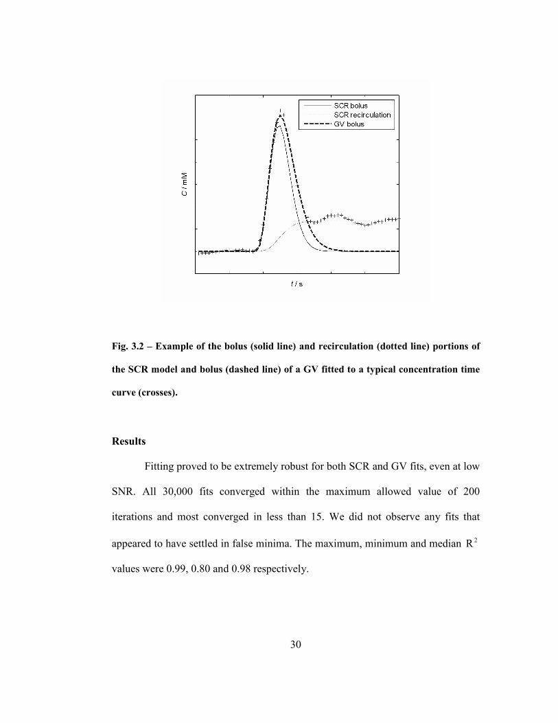
Fig. 3.2 – Example of the bolus (solid line) and recirculation (dotted line) portions

of the SCR model and bolus (dashed line) of a GV fitted to a typical concentration

time curve (crosses)..................................................................................................30

Fig. 3.3 – Fits (line) to concentration time curves (crosses). The left column gives

the “noiseless” concentration time curves and the right has added noise to give an

SNR of 25.................................................................................................................32

xiii

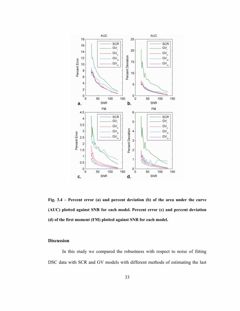
Fig. 3.4 – Percent error (a) and percent deviation (b) of the area under the curve

(AUC) plotted against SNR for each model. Percent error (c) and percent deviation

(d) of the first moment (FM) plotted against SNR for each model..........................33

Fig. 4.1 – *

2T -weighted DSC MRI image acquired at 3 T. Region of interests and

single pixels were drawn to measure signal intensities in, WM, normal appearing

white matter; and GM, caudate nucleus. ..................................................................51

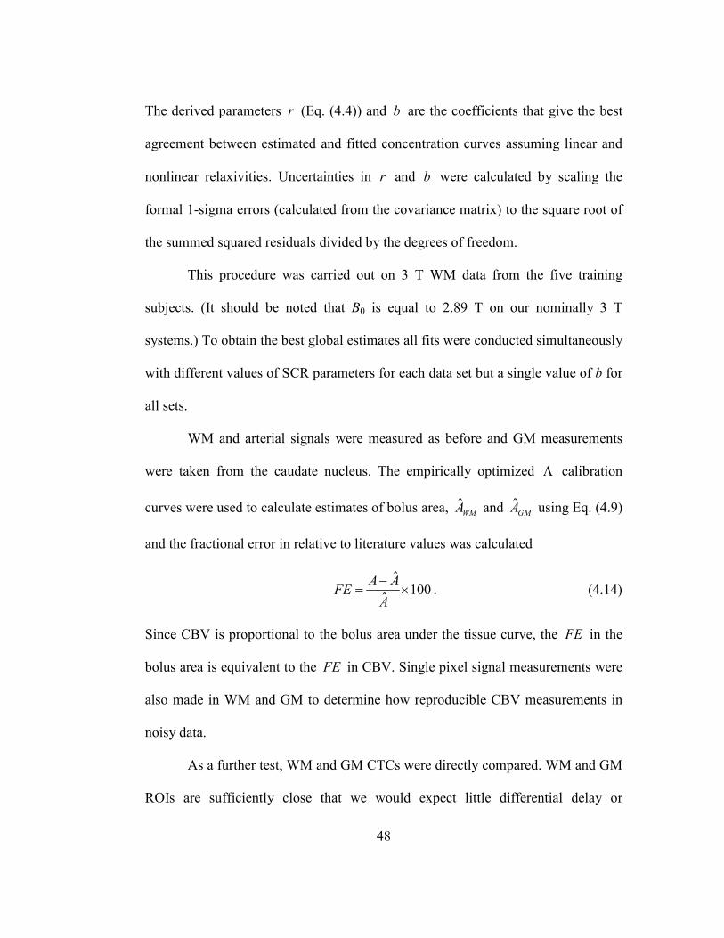
Fig. 4.2 – Plots of measured (+) and fitted values of log ratio, λ . Each plot is the

concatenation of 5 data sets at 3 T, ET = 32 ms. a) Linear formulation. b) Nonlinear

formulation...............................................................................................................52

Fig. 4.3 – Plots of Λ vs. C for the optimized linear (dashed) and SDR (solid)

formulations ( 0B = 3 T; ET = 32 ms). .....................................................................52

Fig. 4.4 – Plots of estimated blood contrast agent concentration from a single

patient at a) 1.5 T and b) 3 T. The concentration estimates were obtained from

signals in arteries (red line), white matter using the linear (blue line) and nonlinear

(green line) formulations. The arterial and white matter concentrations calculated

using the nonlinear formulation is in excellent agreement when considering delay

and dispersion. .........................................................................................................53

Fig. 4.5 – Box and whisker plots of fractional error in ROI and single pixel

measurements in white matter (a and b) and grey matter (c and d) CBV estimates

obtained using the linear and nonlinear formulations at 1.5 T and 3 T. In each box,

the central line represents the median of measurements in five test patients, the

xiv

upper and lower boundaries of the box represent the upper and lower quartiles and

the whiskers represents the range.............................................................................54

Fig. 4.6 – Blood concentration-time curves in WM (blue) and GM (green) from a

single test patient calculated using linear and non-linear formulations at 1.5 T (Figs.

4.6a and e) and 3 T (Figs. 4.6c and g), respectively. Differences between scaled

GM and WM curves from the beginning of the bolus to 30 seconds after are plotted

against WM concentration over all test patients at using linear and non-linear

formulations at 1.5 T (Fig. 4.6b and f) and 3 T (Fig. 4.6d and f), respectively. ......56

Fig. 5.1 – Measured (points) and fitted (solid lines) venous signal intensity time

curves from five patients at 1.5T (a) and 3 T (b). The fitted curves were calculated

using the relaxivity parameters that gave the best agreement between the area under

the bolus, and steady state amplitude of arterial and venous concentration time

curves. .....................................................................................................................71

Fig. 5.2 – Arterial (red) and venous (in vitro – black; in vivo – blue) relaxivity

calibration curves at 1.5 T (a) and 3 T (b). Curve coefficients are given in Table

5.1. ...........................................................................................................................72

Fig. 5.3 – Arterial and venous CTCs at 1.5T (a) and 3T (b). The discontinuities in

the in vitro venous curves are because the same value of *

2R∆ corresponds to two

different concentrations below about 2 mM (see Fig. 5.2). The curve was therefore

obtained by interpolation between zero and the first unambiguous value of *

2R∆ ..73

xv

Fig. 6.1 – Perfusion parameters for the different subject groups measured pre-

(deep gray) and post-treatment (light grey). White and grey matter measurements

are given in the top and bottom rows respectively. Statistically significant

differences are indicated by asterisks (p values can be found in Table 6.2). ...........83

Fig. 6.2 – Fractional rates of change of each parameter per month (i.e., the vertical

scale is in units of month-1) for CBF (left), CBV (middle) and MTT (right) for

white (top) and grey (bottom) matter. Rates of change that are significantly non-

zero are marked by an asterisk (p values can be found in Table 6.3). .....................85

Fig. 7.1 – Cell suspension signal intensities with 4 mM Gd-DTPA versus a: the

MFC refocusing pulse shift ( st ≤ 8 ms), b: IT in 1T measurements ( ≤ 1000 ms),

c: ET in 2T measurements ( ET ≤ 67 ms), and d: ET in *

2T measurements ( ET ≤ 60

ms). The lines are fits to Eq. (7.6) (a), Eq. (7.7) (b) and Eq. (7.8) (c, d). Standard

error estimates for all data points are shown with error bars. ..................................98

Fig. 7.2 – MFC (a) and relaxation rates 1R (b), 2R (c) and *

2R (d) plotted against

Gd-DTPA concentration for cell suspensions and water phantoms. MFC in the cell

suspensions is fitted to a quadratic polynomial. In the relaxation rate plots, solid

and dashed lines represent a linear extrapolations, based on the [Gd] = 0 and [Gd] =

1 mM data points for the cell suspension and water phantom respectively. Standard

error estimates for all data points are shown with error bars. ..................................99

Fig. 7.3 – Plot of MFC difference as a function of Gd-DTPA concentration (Eq.

(7.4)).......................................................................................................................100

xvi

Fig. 7.4 – Bland-Altman plots for MFC (a) and relaxation rates 1R (b), 2R (c) and

*

2R (d). The y axis represents the difference and the x axis the mean of estimated

and true Gd concentrations respectively. The solid line indicates the mean

difference and the dashed lines show ± 95% limit agreements (i.e., approximately

twice the standard deviation of the difference). .....................................................101

xvii

LIST OF TABLES

Table 4.1 – Fractional error in white and grey matter CBV estimates (%) relative to

literature values by the linear and nonlinear equations at 1.5 and 3T for both ROI

and single voxel measurements................................................................................55

Table 5.1 – Relaxivity coefficients for Eq. (5.3) (curves shown in Fig. 5.2)...............72

Table 6.1 – Patient demographics for each group....................................................83

Table 6.2 – The values of each perfusion measure (Mean ± SD) at the last time

point pre-treatment and the first time point post-treatment; the change in value and

the p value from a paired sample t test. Units are as follows: CBF, ml/100 g/min;

CBV, ml/100g; MTT, s. Statistically significant changes are shown in bold..........84

Table 6.3 – Fractional rates of change of each parameter per month in serial

measurements. Statistically significant results are shown in bold. CBV declined at a

statistically significant rate after treatment with bevacizumab. No other rates of

change were significantly different from zero. Note that pre-treatment rates of

change were only available in recurrent glioma patients, Group III, since only a

single initial pre-treatment scan was available for each newly diagnosed patient...86

xviii

LIST OF APPENDICES

APPENDIX A ........................................................................................................108

APPENDIX B ........................................................................................................111

APPENDIX C ........................................................................................................113

1

INTRODUCTION

A Brief History on Measuring Perfusion

In 1897 G.N. Stewart attempted to develop a method to measure cardiac

output applicable to animals of any size (1). Stewart’s motivation came from the

large discrepancies in estimates between previous studies dating back to 1850.

Before Stewart’s study, measuring cardiac output in animals (rabbits, dogs and

horses) employed rather crude methods. Direct measurements involved cutting off

circulation by ligature and measuring the amount of blood passing through the

system (2) or inserting a rheometer in the aorta (3). Indirect measurements

estimated the amount of oxygen added to blood as it passed through the lungs (4)

using the Fick principle – blood flow is proportional to the difference in

concentration of a substance in blood as it enters and leaves an organ (5). Stewart

had the idea of injecting an indicator (sodium chloride) directly into an

anaesthetized dog, taking samples of blood before and after injection during crucial

time points, and then quantifying the amount of indicator in each sample by the

Kohlrausch method – an ingenious method which measures electrolyte resistance in

a solution by a Wheatstone bridge connected to a telephone. Stewart’s

groundbreaking paper paved the way for thousands of future studies measuring

perfusion by means of an indicator.

2

The first study measuring blood flow in the human brain was conducted by

S.S. Kety and C.F. Schmidt in 1945 (6). Subjects were instructed to inhale a

mixture of gas consisting of 15% nitrous oxide and 85% oxygen through an

anesthesia mask for 20 minutes. Nitrous oxide was used because it is

physiologically inert, capable of diffusing across the blood-brain barrier and

quantifiable in blood. During 2, 4, 6, and 10 minute intervals samples of arterial

and venous blood were taken from the femur and right internal jugular vein,

respectively, and the volume of nitrous oxide in the samples are quantified. Then

finally cerebral blood flow was calculated using the Fick principle.

In the early 1960s regional cerebral blood flow measurements could be

made using radioactive indicators. In 1961 N.A. Lassen and D.H. Ingvar injected a

saline and krypton85

solution into cats to detect low energy beta particles with a

Geiger-Muller tube (cats underwent a craniotomy and resection of the dura before

injection). One of the first studies to measure cerebral blood flow with nuclear

medicine in humans was conducted by D.H. Ingvar et al. in 1965 (7). Xenon133

was

injected into the internal carotid artery and the emitted gamma-rays are measured

externally using a scintillation detector around four regions of the brain. Although

using radioactive isotopes to measure perfusion invasively has its advantages i.e. it

is inexpensive and easy to conduct, there are a number of disadvantages both in

methodology and quantification. The topographical detection field cannot be

precisely defined which may result in overlapping counts between regions.

3

Quantitatively, clearance curves exhibit multi-exponentiality making it difficult to

determine an accurate extraction curve (8).

Invasive methods started giving way to noninvasive methods for sampling

indicator, and with the advent of proton emission tomography (PET) by D.E. Kuhl

and colleagues in the 1960s (9), cerebral blood flow measurements could be

quantified from images which displayed indicator concentration levels. PET

imaging is conducted by intravenously introducing a diffusible radioactive

indicator which is converted into a biologically useful molecule, waiting a short

period of time (~2-120 min) until the tracer has reached a substantial concentration

in the tissue of interest and then imaging to measure the indicator concentration as

it decays.

PET provides important clinical information regarding metabolic

functionality and is still considered the “gold standard” for measuring blood flow,

but there are a number of disadvantages. The radioactive indicators may be

dangerous to patients who are sensitive to radiation – it is generally advised for

women who are pregnant or breast feeding to avoid PET scans. Compared to other

imaging modalities, PET is expensive and provides low spatial resolution.

Furthermore, a typical PET scan lasts between ~45-60 min making it

uncomfortable for the patient who is expected to be lying still.

Another imaging modality able to measure perfusion is computerized

tomography (CT). CT was first developed by G.N. Hounsfield in 1973 (10), and a

well formulated theory for estimating perfusion via CT was presented by L. Axel in

4

1980 (11). By the early 1990s, perfusion measurements could be estimated using

conventional CT scanners, and with the introduction of fast multi-detector CT in

the late 1990s, measuring perfusion via CT became a practical clinical technique

(12). Perfusion CT is typically conducted by administering an iodinated contrast

agent (CA) intravenously and dynamically imaging the anatomy of interest as the

first-pass moves through the vasculature.

The main advantages of perfusion CT: 1) wide availability of scanners and

commercial perfusion analysis software. 2) Simplicity of contrast enhancement

quantification – iodinated contrast medium has a linear relationship with X-ray

attenuation. 3) Repeatability and relatively low inter-operator variability. Of course,

the main disadvantage of CT (or any technique dependent on ionizing radiation) is

radiation exposure to the patients. This can be further exacerbated by attempting to

increase the already limited anatomical coverage.

5

Fig. I.1 – Portrait of G.N. Stewart.

Fig. I.2 – Portraits of S.S. Kety (left) and C.F. Schmidt (right)..

6

Perfusion Imaging with MRI

The basis of magnetic resonance imaging (MRI) is nuclear magnetic

resonance (NMR) which was first described by F. Bloch and E. Purcell in 1946.

Both won the 1952 Nobel Prize for Physics. Bloch and Purcell independently found

that certain atoms absorbed energy in the radiofrequency (RF) range when placed

in a magnetic field and emanated this same energy when returning back to their

original energy state. In 1973 the physics of NMR was adapted by P. Lauterbur and

Sir P. Mansfield, the inventors of what we know to be MRI, and were awarded the

2003 Nobel Prize for Physiology or Medicine.

In short, MRI works by exploiting the unique magnetic properties of the

body’s tissue to create high resolution images without the use of radiation. When a

sample abundant in water is placed in a high magnetic field (on the order of 105

times stronger than the Earth’s), the hydrogen nuclei align along the direction of

the external magnetic field. RF energy tuned to the exact resonating frequencies of

the nuclei is deposited in the sample – spatial resolution is obtained by altering the

strength of local magnetic fields using gradient coils. Once the transmitting RF

energy source is turned off, the affected nuclei emit RF energy while returning to a

resting state. The emitted energy is detected by receiver coils placed around the

sample and is used to construct MRI images. The time it takes for the nuclei to

return to a resting state is termed “relaxation rate” and is measured in two

components, longitudinal and transverse. Because tissues have distinct intrinsic

7

relaxation rates, the imaging protocol can be altered to emphasize a particular tissue

in an MRI image.

There are two main types of techniques for measuring perfusion using MRI,

one which utilizes an endogenous and another which uses exogenous indicator.

Arterial spin labeling (ASL), uses labeled blood as an endogenous indicator and

was first introduced by Williams et al. in 1992 (13). A general overview of the

method is as follows: First, water molecules in arterial blood which feeds the tissue

of interest are labeled by inverting their magnetization. Next, an image is acquired

as the labeled molecules enter the tissue of interest and then subtracted from

another image of the same tissue of interest but without the labeled molecules.

Since the absolute signal intensity difference is small, the experiment is repeated

multiple times and perfusion maps are calculated using equations which relate

cerebral blood flow to changes in magnetization. Many derivatives of the initial

ASL method have been proposed and researchers continue to improve the

technique especially with higher field strength scanners. Despite the advancements

in technique and use of an endogenous indicator, ASL is not routinely used in the

clinic. This is because of the low level of perfusion signal (approximately 2% of the

raw signal) compared to the noise levels due to the rapid decay of labeled

molecules. The high noise levels produce large random errors in the blood flow

calculations (14).

The two methods which uses an exogenous indicator are dynamic, contrast-

enhanced (DCE) and dynamic, susceptibility-weighted, contrast-enhanced (DSC)

8

MRI. The main advantages of contrast based MRI versus ASL is a substantially

higher signal-to-noise (20-200) and ability to image a larger portion of the brain.

Both contrast based MRI methods are typically performed by acquiring a series of

images ( 1T for DCE and *

2T for DSC) before, during and after an injection of a

paramagnetic CA called, gadolinium diethylenetriaminepentaacetic acid (Gd-

DTPA). The series of images are used to construct signal-time curves and then are

transformed into concentration-time curves which are used in both DCE and DSC

MRI analyses. DCE data is mainly used for pharmacokinetic modeling (calculating

vasculature permeability and transK , the volume transfer constant between blood

and extracellular-extravascular space) while DSC data is used in first-pass

perfusion analysis to calculate absolute and relative cerebral blood volume (CBV),

flow (CBF), and mean transit time (MTT) – the average time the CA remains in the

tissue. DSC MRI will be the focus of this thesis.

DSC MRI was first developed in the late 1980s and early 90s by Rosen et

al. (15) and is used to assess the hemodynamics of patients suffering from brain

tumors (16-18), ischemia (19,20) and multiple sclerosis (19,21). Previous studies

have shown that perfusion measurements made via DSC MRI can be used to grade

tumors (22), quantitatively assess the degree of angiogenesis (23), guide directed

biopsy (24) and evaluate the efficacy of anti-cancer therapies (25).

There are five main steps when performing a quantitative DSC MRI

experiment.

9

1) Acquiring a series of images with a temporal resolution on the order of

approximately 1 second before, during, and after a bolus of contrast agent is

administered intravenously. Scan times usually range from 1-3 minutes and

the first-pass of the contrast agent is the primary focus of analysis.

2) Making signal measurements to produce signal-time curves in an artery and

in tissue which is further discussed in chapter 2.

3) Converting signal measurements to estimates of contrast agent

concentration. Inaccurate estimates of concentration propagate throughout

the entire subsequent analysis and are arguably the largest source of error.

This step is the main focus of this thesis.

4) Modeling the first-pass by an analytical function to smooth the raw data,

quantify the amount tracer injected and to reduce the effects of contrast

agent leakage and recirculation (these effects, if great, can invalidate

analysis). This is the subject of chapter 3. Modeling the first-pass simplifies

the final step.

5) Calculating perfusion parameters. The equations necessary for calculating

absolute CBV, CBF and MTT will be presented in chapter 1.

A major issue with quantitative DSC MRI is the poor reproducibility and accuracy

of perfusion measurements in tissue. Lack of reproducibility has obvious

consequences for the sensitivity and specificity for DSC based diagnoses. Lack of

accuracy prevents meaningful comparison of results from different modalities e.g.

PET or CT, and between MRI studies using different imaging protocols. For

10

example, the optimal rCBV cutoff for distinguishing low and high grade gliomas has been

reported as anywhere between 1.5 and 5.6 (26-30).

Therefore, the overarching aim of the work presented in this thesis is to

improve the reproducibility and accuracy of DSC methods.

Fig. I.3 – Portraits of F. Bloch (top left), E. Purcell (top right)†, P. Lauterbur

(bottom left) and Sir P. Mansfield (bottom right)‡.

† “The Nobel Prize in Physics 1952”. Nobelprize.org 9 Apr 2013

http://www.nobelprize.org/nobel_prizes/physics/laureates/1952/ ‡ “The Nobel Prize in Physiology or Medicine 2003”. Nobelprize.org 9 Apr 2013

http://www.nobelprize.org/nobel_prizes/medicine/laureates/2003/

11

CHAPTER 1: On the Theory of Measuring Perfusion

The Central Volume Theorem

It took twenty-four years after G.N. Stewart’s 1897 study when he realized

that no study had measured the minute volume in the heart, V , volume of blood in

the lungs, Q , and the mean pulmonary circulation time, M , in the same animal. In

1921, G.N. Stewart achieved the aforementioned and determined that if two of the

quantities are know then by the following relationship,

V QM= (1.1)

the third can be calculated (31).

As more sophisticated injection techniques developed, so did the

understanding of the mathematical basis of indicator-dilution methods. In 1931,

W.F. Hamilton et al. conducted experiments on humans which involved injecting

an indicator (dye) and then using a 19 G. needle to collect serial samples of blood

every 1-2 seconds from the femoral artery. The concentration of dye was

determined colorimetrically, plotted against time and then a smooth curve was fit

by hand through the data points thus giving rise to a concentration-time curve

(CTC). From the CTC, flow, F , and mean circulation time, M , can be calculated

n n

n

c tmF M

ct c= = ∑ (1.2)

12

where m is the mass of dye, c is the average concentration during the first bolus

pass, t is the time during the first bolus pass and nc and nt are the concentration

and times at the nth reading, respectively. The volume of the system, V , can then

be calculated using what is known as the central volume theorem:

V FM= (1.3)

A proof of the central volume theorem can be found in Appendix A.

Applying the Intravascular Indicator Dilution Theory to DSC MRI

In 1954 P. Meier and K.L. Zierler provided the first direct mathematical

proof of Eq. (1.3) considering both an instantaneous and constant fusion under the

following assumptions which make up the intravascular indicator dilution theory

(32). 1.) Stationarity of flow – indicator entering a system will be dispersed exiting

the system in the same manner as indicator entering the system at any other time.

This assumption will be violated in systems where volume and flow change

phasically, like the heart. 2.) Flow of indicator in a system is representative of the

flow of the fluid in the system. 3.) There are no stagnant pools in the system. 4.)

Recirculation is not present. It is apparent that depending on the injection protocol,

some of the aforementioned assumptions will be violated. If the injection is

instantaneous and the system displays non-stationarity properties then the injection

time and phasic cycle must be taken into account which may lead to unreliable

measurements. However, measurements may be insensitive using a constant

infusion in a non-stationary system. Conversely, depending on the length of the

13

system, recirculation effects may be introduced in measurements if the injection is

constant (i.e. constant infusion); in which case perhaps an instantaneous injection

would be most advantageous.

The central equation for a DSC MRI experiment is

( ) ( ) ( )Ht a

kC t FC t R t

ρ= ⊗ (1.4)

where ( )aC t is contrast agent concentration estimated from an artery feeding a

tissue of interest, ( )tC t . Hk is a constant which accounts for the difference

between arterial and capillary hematocrit, ρ is the tissue density, ⊗ denotes

convolution, F is CBF and ( )R t is the residue function to be defined below. It

should be noted that in much of the literature ρ is ignored since it is very close to

unity. However, it is necessary for Eq. (1.4) to be dimensionally correct.

Eq. (1.4) can be derived by the following equations. The volume of blood

(i.e. CBV), bv , entering a volume of tissue, tV , in time dτ is

Hb t

kv FV dτ

ρ= (1.5)

where F is in standard units of mL/100 g of tissue/min. The quantity of indicator,

q , entering tV at time τ is then

( )Ha t

kdq FC V dτ τ

ρ= (1.6)

14

and the amount of indicator remaining at time t , by the definition of ( )R t – the

residue function, is

( ) ( ) ( )dq t dq R tτ τ= − . (1.7)

Thus, the total quantity of indicator at time t is then obtained by integrating Eq.

(1.7) between τ = 0 and t

( ) ( )0

tH

t a

kq FV C R t dτ τ τ

ρ= −∫ , (1.8)

and can be rewritten as a convolution

( ) ( ) ( )Ht a

t

kqC t FC t R t

V ρ= = ⊗ . (1.9)

F and ( )R t can be calculated by deconvolution methods discussed in the next

chapter.

To calculate the mean transit time, MTT in standard units of s (i.e. M in

the previous section), it can be proven that

( )0

MTT R t dt∞

= ∫ . (1.10)

A proof of Eq. (1.10) can be found in Appendix B.

The central volume theorem (Eq. (1.3)) can now be written in terms of

absolute DSC MRI perfusion measurements to calculate CBV:

CBV CBF MTT= ⋅ . (1.11)

Alternatively, CBV can be calculated in standard units of mL/100 g of tissue using

the following equation,

15

( )( )

CBVtH

a

C t dtk

C t dtρ= ∫

∫ (1.12)

A proof of Eq. (1.12) can also be found in Appendix B.

16

CHAPTER 2: Fundamentals of Quantitative DSC MRI

Image Acquisition

Images for a DSC MRI experiment can be acquired using single or multi-

shot gradient or spin echo echo planar imaging (EPI) – the vast majority of DSC

MRI studies are performed using single-shot gradient echo EPI to create *

2T -

weighted images and will only be considered throughout this document. These

pulse sequences are able to produce temporal resolutions (i.e. the repetition time,

RT ) of ~1 s, are able to cover 5-12 slices with a matrix size of 128×128 and a

resolution of ~1.8×1.8 mm2 . The echo time, ET , ranges from 30-50 ms and the flip

angle, FA , ranges from 30-90° with a slice thickness of 3-5 mm. Gd-DTPA is

injected at a dose of 0.1-0.2 mmol/kg at a rate of 5 mL/s followed by a 10 mL bolus

of saline to flush any residual contrast agent in the blood stream. Typically, the

total image acquisition time is 1-3 min and starts ~10 s before the bolus arrival

time.

Signal Theory

The essential first step in quantitative DSC MRI is the conversion of signal

intensity as a function of time, ( )S t , to Gd-DTPA concentration, ( )C t , and are

related by the following equation

17

( ) ( )( )( ) ( )( )( )

( ) ( )( )( ) ( )

( ) ( )1 1 1 1*

0 2 * *1 2 2

sin 1 exp 0exp ;

1 cos exp

R

E

R

FA R t T R t R rCS t S R t T

FA R t T R t r C t

− − = += −∆

− − ∆ =

where 0S is a constant describing proton density and scanner gain, ( )*

2R t∆ is the

change in transverse relaxation rate ( * *

2 21R T≡ ) due to the presence of ( )C t , *

2r is

a proportionality constant (a.k.a. the relaxivity constant) and 1r is the relaxivity

constant used to relate ( )C t to longitudinal relaxation rate, 1R ( 1 11R T≡ ).

Fortunately, 1T effects can be ignored if imaging parameters, such as FA

and ET , are chosen to minimize 1T sensitivity (reducing FA and increasing ET ).

Dropping the 1T contribution from the equation above and substituting ( )CΛ , a

unitless function describing the change in *

2T due to the presence of CA, for *

2 ER T∆

yields,

( ) ( )( )exppreS t S C= −Λ (2.1)

where preS is the average signal intensity before the bolus arrives. Eq. (2.1) is

considered the fundamental signal equation for a DSC MRI experiment.

The transverse relaxation rate ( *

2T ) is affected by two processes:

microscopic dipole-dipole interactions and “mesoscopic” interactions due to

magnetic field perturbations caused by tissue structures in close proximity with

differing susceptibilities. The mesoscopic effects are determined by

compartmentalization of Gd-DTPA (that is to say CA in blood vessels) which

creates susceptibility gradients between the vessel and surrounding tissue. Water

18

molecules lose phase coherence as they diffuse through these manufactured

gradients, resulting in shorter *

2T and in turn a decrease in signal intensity (33-35).

Before any DSC MRI analysis, signal measurements from arterial and tissue

must be made. Generally, arterial voxels are detected either manually or

automatically. Manual detection is conducted by an experienced researcher or

radiologist who determines individual signal-time series curves which appear to fit

the profile of an arterial voxel (large signal drop, early bolus arrival and narrow

bolus). Automatic detection entails implementing an algorithm which screens each

voxel and selects the likeliest arterial candidates (36-38). In some instances,

multiple arterial signals are averaged to increase SNR. Tissue measurements are

made by drawing regions of interest (ROI) around a tissue of interest. ROIs

encompass ~10 voxels and are averaged. Alternatively analysis may be performed

on every voxel to create perfusion maps. Once signal measurements are made, Eq.

(2.1) can be used to calculate ( )aC t and ( )tC t , and finally CBV, CBF and MTT

can be calculated.

Deconvolution

Eq. (1.4), ( ) ( ) ( )Ht a

kC t FC t R t

ρ= ⊗ , is considered an ill-posed convolution

equation because both F and ( )R t are unknown ( Hk

ρ is an estimated constant and

will be omitted from following equations for simplicity but it is imperative that it is

19

taken into account during all analyses). There are two approaches for solving Eq.

(1.4), either by assuming or not assuming a known function to model ( )R t . The

model dependent approach generally assumes an exponential or Lorentzian

function for ( )R t as a function of MTT (for example ( ) t MTTR t e−= ) and uses

general nonlinear least squares minimization to calculate F and MTT (39,40). This

approach is usually taken during computer simulations, however in practice a

model independent approach is taken due to the uncertainty in assuming a model

for ( )R t .

The two main methods for model independent deconvolution are

transformation and an algebraic approach. Transformation uses the convolution

theorem of Fourier i.e. the transform is multiplicative to convolution. Thus, F and

( )R t can be solved by the following equations ( { }f̂ denotes the Fourier

transform and its inverse, { }1f̂ − ),

( ){ } ( ){ } ( ){ }ˆ ˆ ˆt af C t Ff C t f R t= (2.2)

which can be rearranged to show,

( )( ){ }( ){ }

1ˆ

ˆˆ

t

a

f C tFR t f

f C t

−

=

. (2.3)

This approach is time efficient and easy to implement from a computational

standpoint but is severely sensitive to noise. For this reason a Weiner filter and

other dampening filters must be used to reduce noise sensitivity (36,41).

20

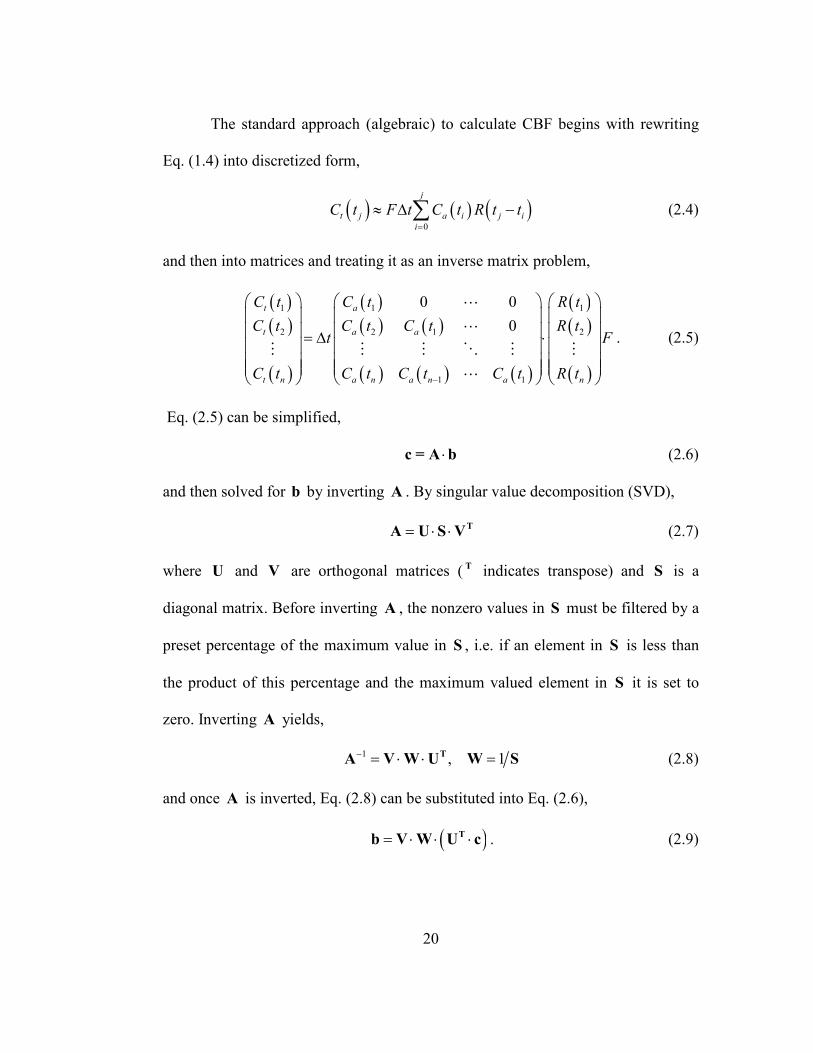
The standard approach (algebraic) to calculate CBF begins with rewriting

Eq. (1.4) into discretized form,

( ) ( ) ( )0

j

t j a i j i

i

C t F t C t R t t=

≈ ∆ −∑ (2.4)

and then into matrices and treating it as an inverse matrix problem,

( )( )

( )

( )( ) ( )

( ) ( ) ( )

( )( )

( )

1 1 1

2 2 1 2

1 1

0 0

0

t a

t a a

t n a n a n a n

C t C t R t

C t C t C t R tt F

C t C t C t C t R t−

= ∆ ⋅

⋯

⋯

⋮ ⋮ ⋮ ⋱ ⋮ ⋮

⋯

. (2.5)

Eq. (2.5) can be simplified,

⋅c = A b (2.6)

and then solved for b by inverting A . By singular value decomposition (SVD),

= ⋅ ⋅ TA U S V (2.7)

where U and V are orthogonal matrices ( T indicates transpose) and S is a

diagonal matrix. Before inverting A , the nonzero values in S must be filtered by a

preset percentage of the maximum value in S , i.e. if an element in S is less than

the product of this percentage and the maximum valued element in S it is set to

zero. Inverting A yields,

1 , 1− = ⋅ ⋅ =TA V W U W S (2.8)

and once A is inverted, Eq. (2.8) can be substituted into Eq. (2.6),

( )= ⋅ ⋅ ⋅Tb V W U c . (2.9)

21

Because b is scaled by F , it can be calculated by taking the maximum value of b

(40).

To improve the standard SVD approach, advanced algebraic techniques

have been investigated such as block-circulant deconvolution (42) and

regularization (43,44).

Sources of Quantification Error

There are many errors that can influence DSC MRI estimates such as the

deconvolution process (42,45-47) and the effects of CA leakage into extracellular-

extravascular space on signal (48,49). Another source of error comes from arterial

measurements. Even if relatively large arteries such as the middle cerebral artery

are sampled, the resolution is sufficiently low that sampled “arterial” voxels are

likely to be contaminated by brain parenchyma. The two major issues addressed by

the following chapters are outlined below.

The first source of error is modeling the first-pass bolus as an analytical

function. This is important because it smoothes raw data and simplifies perfusion

quantification (see Eq. (1.12)). The errors concerning the aforementioned along

with a practical solution will be discussed in chapter 3.

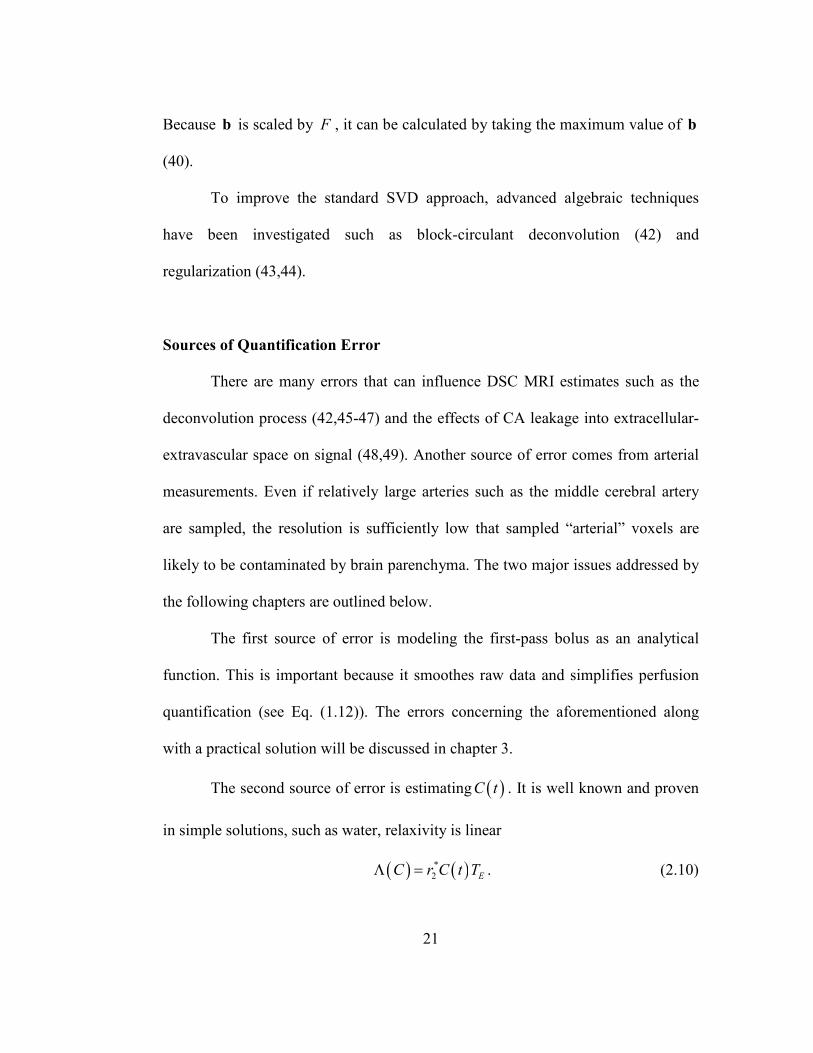
The second source of error is estimating ( )C t . It is well known and proven

in simple solutions, such as water, relaxivity is linear

( ) ( )*

2 EC r C t TΛ = . (2.10)

22

However, in heterogeneous material such as tissue, blood and yeast the relationship

is decidedly nonlinear (34,35,50-59). The exact magnitude of these errors are

unknown, however Calamante et al. suggest that the effects on relative perfusion

measurements may be small when compared to absolute (60). The relaxivity in

arterial blood has been empirically determined using bulk blood phantoms and

follows a quadratic form,

( ) ( )2

EC pC qC TΛ = + (2.11)

where p and q are coefficients which depend on factors such as hematocrit and

field strength (53,54). The relaxivity of tissue, venous blood and yeast will be

further investigated in chapters 4, 5 and 7, respectively.

23

CHAPTER 3: The Single Compartment Recirculation Model

The work in this chapter appears in Medical Physics under the following citation:

Patil V, Johnson G. An Improved Model for Describing the Contrast Bolus in

Perfusion MRI. . Med Phys 2011;38(12):6380-6383.

This study was funded in part by NIH grant RO1CA111996.

Author Contributions:

Vishal Patil – Project concept and design, data acquisition and analysis,

manuscript drafting and revisions.

Glyn Johnson – Project concept and design, manuscript drafting and

revisions, final approval for publication.

24

Abstract

Quantification of perfusion measurements using dynamic, susceptibility-

weighted contrast-enhanced (DSC) MRI depends on estimating the size and shape

of the tracer bolus. Typically, the bolus is described as a gamma variate function fit

directly to the tracer concentration time curve (CTC), however, there are problems

associated with this method. First, the last point to fit is arbitrary and more

importantly, direct fitting also includes a portion of the recirculation curve, which

in turn overestimates and distorts the true bolus. In this study, we present a model

which also describes the bolus as a gamma variate but takes into account

recirculation during the bolus and is fit to the entire CTC.

25

Introduction

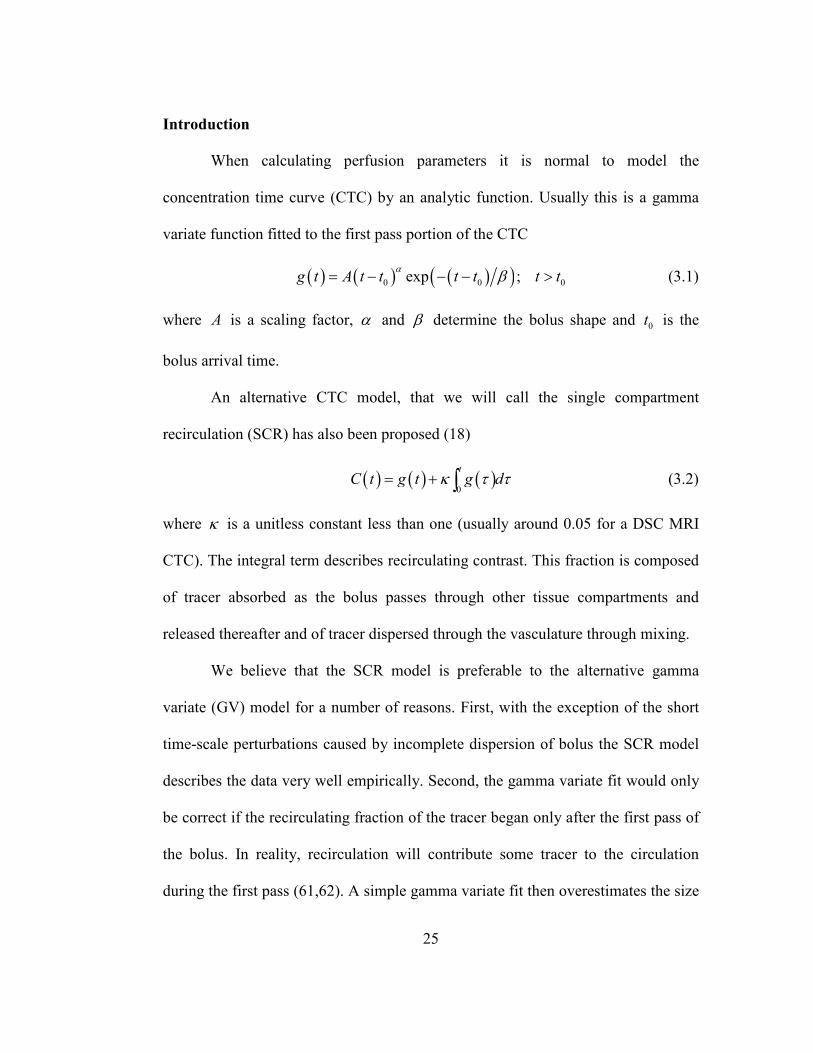
When calculating perfusion parameters it is normal to model the

concentration time curve (CTC) by an analytic function. Usually this is a gamma

variate function fitted to the first pass portion of the CTC

( ) ( ) ( )( )0 0 0exp ;g t A t t t t t tα β= − − − > (3.1)

where A is a scaling factor, α and β determine the bolus shape and 0t is the

bolus arrival time.

An alternative CTC model, that we will call the single compartment

recirculation (SCR) has also been proposed (18)

( ) ( ) ( )0

t

C t g t g dκ τ τ= + ∫ (3.2)

where κ is a unitless constant less than one (usually around 0.05 for a DSC MRI

CTC). The integral term describes recirculating contrast. This fraction is composed

of tracer absorbed as the bolus passes through other tissue compartments and

released thereafter and of tracer dispersed through the vasculature through mixing.

We believe that the SCR model is preferable to the alternative gamma

variate (GV) model for a number of reasons. First, with the exception of the short

time-scale perturbations caused by incomplete dispersion of bolus the SCR model

describes the data very well empirically. Second, the gamma variate fit would only

be correct if the recirculating fraction of the tracer began only after the first pass of

the bolus. In reality, recirculation will contribute some tracer to the circulation

during the first pass (61,62). A simple gamma variate fit then overestimates the size

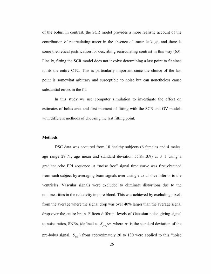
26

of the bolus. In contrast, the SCR model provides a more realistic account of the

contribution of recirculating tracer in the absence of tracer leakage, and there is

some theoretical justification for describing recirculating contrast in this way (63).

Finally, fitting the SCR model does not involve determining a last point to fit since

it fits the entire CTC. This is particularly important since the choice of the last

point is somewhat arbitrary and susceptible to noise but can nonetheless cause

substantial errors in the fit.

In this study we use computer simulation to investigate the effect on

estimates of bolus area and first moment of fitting with the SCR and GV models

with different methods of choosing the last fitting point.

Methods

DSC data was acquired from 10 healthy subjects (6 females and 4 males;

age range 29-71, age mean and standard deviation 55.8±13.9) at 3 T using a

gradient echo EPI sequence. A “noise free” signal time curve was first obtained

from each subject by averaging brain signals over a single axial slice inferior to the

ventricles. Vascular signals were excluded to eliminate distortions due to the

nonlinearities in the relaxivity in pure blood. This was achieved by excluding pixels

from the average where the signal drop was over 40% larger than the average signal

drop over the entire brain. Fifteen different levels of Gaussian noise giving signal

to noise ratios, SNRs, (defined as preS σ where σ is the standard deviation of the

pre-bolus signal, preS ) from approximately 20 to 130 were applied to this “noise

27

free” data. This process was repeated 200 times giving a total of 30,000 different

simulated signals.

CTCs were modeled by both SCR and GV, converted to signal and fitted to

the noisy signal data. Signal, S , was calculated using the standard expression.

Fitting to the signal is preferable because the weighting for each data point is equal

for all signal intensities and because preS can be included as a fitting parameter,

making optimum use of the available data in finding this parameter.

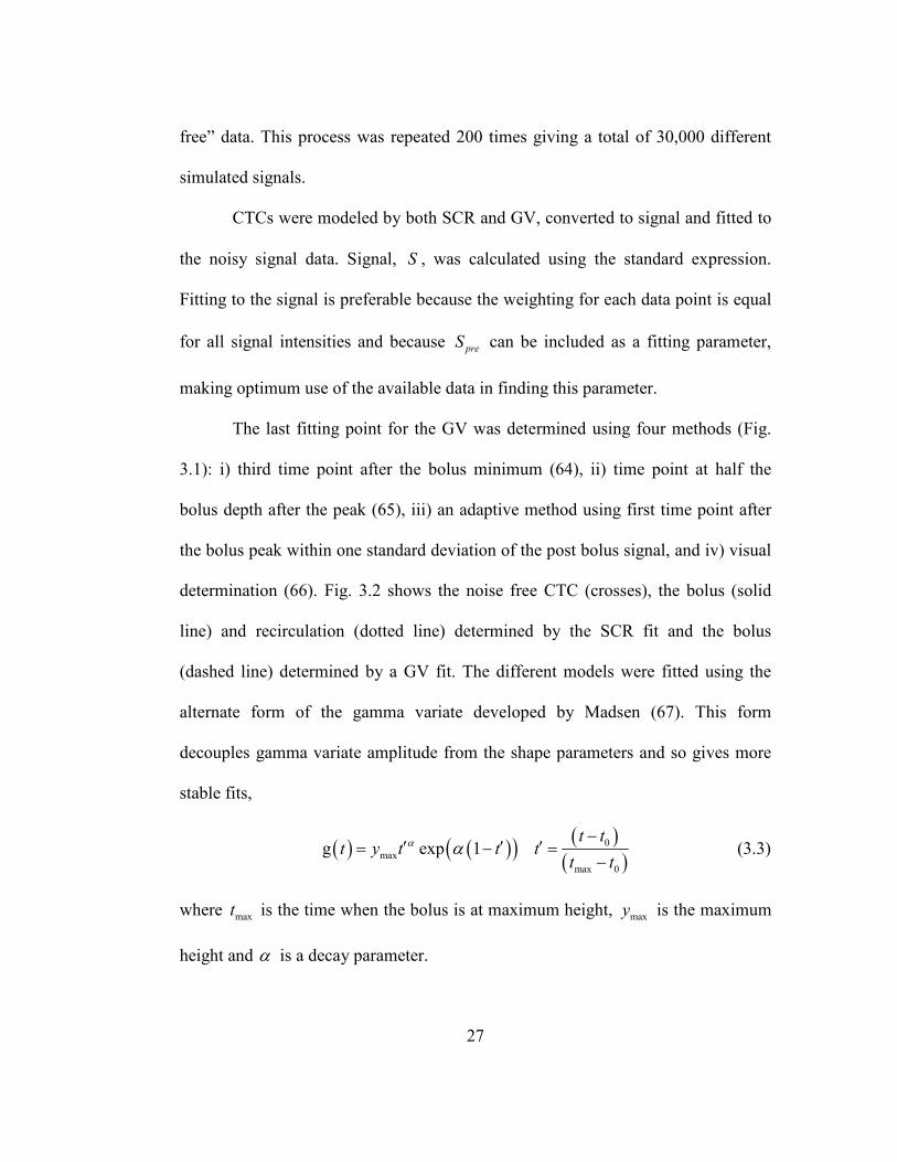
The last fitting point for the GV was determined using four methods (Fig.

3.1): i) third time point after the bolus minimum (64), ii) time point at half the

bolus depth after the peak (65), iii) an adaptive method using first time point after

the bolus peak within one standard deviation of the post bolus signal, and iv) visual

determination (66). Fig. 3.2 shows the noise free CTC (crosses), the bolus (solid

line) and recirculation (dotted line) determined by the SCR fit and the bolus

(dashed line) determined by a GV fit. The different models were fitted using the

alternate form of the gamma variate developed by Madsen (67). This form

decouples gamma variate amplitude from the shape parameters and so gives more

stable fits,

( ) ( )( ) ( )( )

0

max

max 0

g exp 1t t

t y t t tt t

α α−

′ ′ ′= − =−

(3.3)

where maxt is the time when the bolus is at maximum height, maxy is the maximum

height and α is a decay parameter.

28

Next, for each fit the area under the curve (AUC) and the normalized first

moment (FM) of the bolus (i.e., the gamma variate portion of both SCR and GV

models) were calculated using the following equations,

( ) ( )1

maxmax

0AUC 1

tg t dt y

α

αα

+∞ = = Γ +

∫ (3.4)

( )

( )( )0 max

0

0

FM 1tg t dt t

tg t dt

αα

∞

∞= = + +∫∫

(3.5)

where Γ is the gamma function. CBV is proportional to AUC and CBF is a

function of FM so these two parameters determine the errors that poor fits will

introduce into perfusion estimates.

Finally, the percent error (Eq. (3.6)) and percent deviation (Eq. (3.7))

relative to values for the “noiseless” fit, respectively, were calculated

P.E. 100SNR

SNR i

SNR

x x

x

=∞=

=∞

−= × (3.6)

( )21

P.D. 100SNR i

x xN

x=

−= ×

∑ (3.7)

where N is the number of trials.

29

Fig. 3.1 – Diagram of a typical signal time curve illustrating how the last fitted point

for the gamma variate was selected for each method: i) third point after the bolus

minimum, ii) point of the half drop of the bolus after the bolus minimum, iii) the

point after the minimum at which the signal exceeds the post bolus signal minus the

standard deviation of the pre bolus signal (σ ) and iv) by visual determination.

30

Fig. 3.2 – Example of the bolus (solid line) and recirculation (dotted line) portions of

the SCR model and bolus (dashed line) of a GV fitted to a typical concentration time

curve (crosses).

Results

Fitting proved to be extremely robust for both SCR and GV fits, even at low

SNR. All 30,000 fits converged within the maximum allowed value of 200

iterations and most converged in less than 15. We did not observe any fits that

appeared to have settled in false minima. The maximum, minimum and median 2R

values were 0.99, 0.80 and 0.98 respectively.

31

Fig. 3.3 shows typical fits for the SCR model (Fig. 3.3a and b) and for each

GV method (i-iv) (Fig. 3.3c-j) for the “noiseless” data and with noise added to

reduce the SNR to 25.

The percent error and percent deviation of AUC (Fig. 3.4a and b) and FM

(Fig. 3.4c and d) for the different models are plotted against SNR in Fig. 3.4. In

general GVi (third point) performs poorly for both error and deviation. The SCR

model, GVii (half depth) and GViv (visual inspection) give similar errors while

GViii (adaptive) performs acceptably for AUC but poorly for FM. The SCR model

performs as well as the best GV methods for AUC and rather better for FM.

Mean values of AUC and FM were smaller for the SCR model than values

for all gamma variate fitting procedures as one would expect from Fig. 3.2. There

were only small differences between mean values for the different GV methods.

For example at an SNR of 100, SCR AUC and FM were 7.6 ± 1.73 a.u. and 8.8 ±

2.40 s respectively whereas GV values were 9.4 ± 1.88 a.u. and 10.0 ± 2.51 s.

32

Fig. 3.3 – Fits (line) to concentration time curves (crosses). The left column gives the

“noiseless” concentration time curves and the right has added noise to give an SNR of

25.

33

Fig. 3.4 – Percent error (a) and percent deviation (b) of the area under the curve

(AUC) plotted against SNR for each model. Percent error (c) and percent deviation

(d) of the first moment (FM) plotted against SNR for each model.

Discussion

In this study we compared the robustness with respect to noise of fitting

DSC data with SCR and GV models with different methods of estimating the last

34

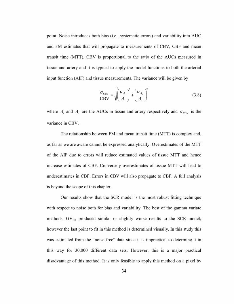
point. Noise introduces both bias (i.e., systematic errors) and variability into AUC

and FM estimates that will propagate to measurements of CBV, CBF and mean

transit time (MTT). CBV is proportional to the ratio of the AUCs measured in

tissue and artery and it is typical to apply the model functions to both the arterial

input function (AIF) and tissue measurements. The variance will be given by

2 2

CBV

CBV

t aA A

t aA A

σ σσ = +

(3.8)

where tA and aA are the AUCs in tissue and artery respectively and CBVσ is the

variance in CBV.

The relationship between FM and mean transit time (MTT) is complex and,

as far as we are aware cannot be expressed analytically. Overestimates of the MTT

of the AIF due to errors will reduce estimated values of tissue MTT and hence

increase estimates of CBF. Conversely overestimates of tissue MTT will lead to

underestimates in CBF. Errors in CBV will also propagate to CBF. A full analysis

is beyond the scope of this chapter.

Our results show that the SCR model is the most robust fitting technique

with respect to noise both for bias and variability. The best of the gamma variate

methods, GViv, produced similar or slightly worse results to the SCR model;

however the last point to fit in this method is determined visually. In this study this

was estimated from the “noise free” data since it is impractical to determine it in

this way for 30,000 different data sets. However, this is a major practical

disadvantage of this method. It is only feasible to apply this method on a pixel by

35

pixel basis if it is assumed that the length of the bolus is the same for all pixels.

Clearly this is not the case and will result in significant errors.

The SCR model corrects for errors that are likely to be smaller than others

often associated with DSC MRI. However many of these errors can also be

addressed effectively by improved processing and acquisition methods. For

example, partial volume effects due to inadequate spatial resolution can be reduced

using reference signals acquired from the sagittal sinus (68); signal “clipping”

(saturation) can be reduced by reducing tracer dose or echo time; and the

nonlinearity between relaxation and concentration can be addressed by using

empirically derived calibration curves (53).

There are a number of limitations of the SCR model and of this study. First,

the model is based on the assumption that recirculation starts at the beginning of

the bolus and increases as a gamma function. Neither of these assumptions can be

fully justified. There may be a delay before recirculation contrast arrives and some

other function may describe its arrival more accurately. Nonetheless the form of

the function must be approximately sigmoidal similar to the form we suggest.

Second, we did not consider the possible effects of cardiac output on our results.

However, our subjects covered a wide age range (29-71) suggesting that cardiac

output has relatively little effect. Third, the SCR model takes no account of errors

introduced by incomplete dispersion leading to second or even third pass peaks.

These errors might be particularly severe if too few measurements are taken after

the bolus so that the steady-state portion of the curve is not reached. We are

36

currently investigating more sophisticated models that explicitly account for

secondary peaks. Conversely, if too many data points are acquired after the bolus,

the steady state portion of the curve will start to decline because of tracer clearance

through the kidneys. However, this can be accounted for by multiplying the SCR

model by an exponential decay term. The model introduces one additional fitting

parameter, κ , giving the possibility of over-fitting and instability. However, the

effect of κ on the shape of the function is so different from those of the other

parameters that this is not a serious risk in practice. Finally, the SCR model is

subject to many of the same errors as the GV model such as tracer leakage, 1T

contamination and partial volume effects.

In conclusion, we have demonstrated that the SCR model gives a more

robust fit in the presence of noise while giving a more realistic representation of

tracer boluses than the gamma variate.

37

CHAPTER 4: *

2R∆ Relaxivity in Brain Tissue

The work in this chapter appears in NMR in Biomedicine under the following

citation:

Patil V, Jensen JH, Johnson G. Intravascular contrast agent T(2) (*) relaxivity in

brain tissue. NMR Biomed 2013;26(4):392-399.

This study was funded in part by NIH grant RO1CA093992.

Author Contributions:

Vishal Patil – Project concept and design, data acquisition and analysis,

manuscript drafting and revisions.

Jens H. Jensen – Project concept and design, manuscript drafting and

revisions.

Glyn Johnson – Project concept and design, manuscript drafting and

revisions, final approval for publication.

38

Abstract

Dynamic, susceptibility-weighted, contrast-enhanced (DSC) MRI perfusion

measurements depend on estimating intravascular contrast agent (CA)

concentration (C ) from signal intensity changes in *

2T -weighted images after bolus

injection. Generally, linearity is assumed between relaxation and C , but previous

studies have shown that compartmentalization of CA and secondary magnetic field

perturbations generate deviations from linearity. Physical phantoms using bulk

blood have been used to empirically determine the relationship between relaxation

rate and C in large vessels. However, the relaxivity of CA in the microvasculature

is not easily estimated since constructing appropriate phantoms is difficult. Instead,

theoretical relaxivity models have been developed. In this study we empirically

tested both linear models of tissue relaxivity and a theoretical model based on the

static dephasing regime. Signal-time curves in white matter (WM) and grey matter

(GM) were converted to concentration-time curves (CTCs) using a nonlinear

expression based on the static dephasing regime (SDR) and a linear approximation.

Parameters for both the linear and nonlinear formulations were adjusted to give the

best agreement between cerebral blood volumes (CBV) calculated from the WM

and arterial CTCs in a group of normal subjects scanned at 3 T. The optimized

parameters were used to calculate blood volume in WM and GM in healthy

subjects scanned at 3 T and in meningioma patients scanned at 1.5 T. Results from

this study show the nonlinear SDR formulation gives an acceptable functional form

39

for tissue relaxivity, giving reliable CBV estimates at different field strengths and

echo times.

40

Introduction

If 1T effects are neglected, the signal, S , in a DSC MRI experiment is

given by

( )( )exppreS S C= −Λ (4.1)

where preS is the signal before contrast injection and ( )CΛ is a function describing

signal loss due to the presence of CA in the vasculature. (It should be noted ( )CΛ

is a unitless function).

In general, CA concentration corresponding to a particular signal is

estimated by first calculating signal log ratios, λ

lnpre

S

Sλ

= −

(4.2)

and applying the inverse of ( )CΛ either analytically or by means of a lookup table:

( )1

0C λ−= Λ Λ + . (4.3)

In most studies a linear relationship between C and relaxation rate is

assumed so that

ErCTΛ = (4.4)

where r is the CA relaxivity constant. However, studies have demonstrated that

this linear relationship, while valid in simple solutions, may fail in more structured

media and thus can lead to systematic errors in C quantification in vivo (57,60).

Worse, relaxivity is generally dependent on both magnetic field and echo time so

that DSC results are protocol dependent and cannot be meaningfully compared

41

across studies. For example, the optimal relative CBV (rCBV) cutoff for

distinguishing low and high grade gliomas has been reported as anywhere between

1.5 and 5.6 (26-30).

The exact expression for relaxivity depends on the compartmentalization of

CA in different tissue types (34,35,51,57,69-72). Studies of gadolinium

diethylenetriaminepentaacetic (Gd-DTPA) in bulk blood (and hence large vessels)

have found a quadratic relaxivity so that (53,55,71,72)

( )2

EpC qC TΛ = + (4.5)

where p and q are constants.

However, tissue microvasculature is difficult to replicate in a physical

phantom and in vivo calibration measurements are difficult to perform. For these

reasons, researchers have resorted to theoretical models and Monte Carlo

simulations to determine tissue CA relaxivity (34,35,69,73). Two theoretical

limiting cases of *

2T relaxivity have been described: the static dephasing regime

(SDR) and the diffusion narrowing regime (DNR). In the latter, the signal

dephasing time is long enough for molecular diffusion to average out phase shifts

caused by different magnetic moments (74). DNR holds when the diffusion length

of a water proton is much greater than the characteristic distance describing the

distribution of contrast agent in tissue. Conversely, the SDR holds when diffusion

lengths are small.

42

The SDR, first formulated by Yablonskiy and Haacke (33) for randomly

oriented cylinders, is divided into short and long dephasing time regimes:

( )

( )

20.3 1.5

1 1.5

E E

E E

T T

T T

ς ω ως ω ω

≤Λ =

− ≥ (4.6)

where

( )0 0kC Bω ηπγ χ= + (4.7)

ς is the tissue vascular fraction, η is a constant that depends on the geometry of

the vasculature network, γ is the gyromagnetic ratio, 0B is the external magnetic

field, 0χ is the magnetic susceptibility due to deoxygenated red blood cells, and k

is a coefficient relating susceptibility to Gd-DTPA concentration. Yablonskiy and

Haacke also give an interpolation formula valid over all ET (33):

( )0

1

20

31

1 22 1

3

EJ T u

u u duu

ως

− Λ = + −∫ (4.8)

where 0J is the zeroth order Bessel function and we have included a simplified

form for ω in the second form of the equation.

A later study by Kjølby et al. using Monte Carlo and suggested that a linear

relationship is adequate to describe relaxivity for ET > 10 ms when using double-

dose contrast (73). However, a more recent simulation study (75) suggests a

nonlinear relationship is more accurate for single dose.

43

The purpose of this study was to determine a functional form for Λ that

allows reliable estimates of C in WM and GM at different field strengths and echo

times. To this end, we compared the full (Eq. (4.8)) and linear approximation (the

long ET approximation of Eq. (4.6)) of the SDR model. Constants in these

equations can be estimated theoretically (33,73) but depend on factors such as

vessel geometry, etc., that are not accurately known. We therefore assumed

ω = rCB

0for the linear model and determined empirically the value of r that gave

the best agreement between tissue and arterial bolus curves in control subjects.

Similarly, we assumed that ω = a + bC( )B0

for the full SDR model and found best

agreement values of a and b . However, during development we observed that the

procedure was very insensitive to the a term giving similarly good fits and similar

b values (within about 2%) when it was constrained to be zero. This lack of

sensitivity can be explained by the shape of the calibration curve (Fig. 4.3).

Altering the value of the constant term shifts the relaxivity curve along the

concentration axis close to the origin. Because the slope of the curve is close to

zero at that point, the change in relaxivity is very small. Our final results were

therefore derived with a set to zero. (Note that although this also gives a linear

relationship between C and ω , Λ is nonlinear with C .)

The empirically determined values of r and b were then validated in WM

and GM at different field strengths and echo times in a different set of subjects.

44

Methods

This retrospective study was approved by our Institutional Review Board.

Data were obtained from 5 meningioma patients scanned at 1.5 T who had

undergone DSC MRI as part of their standard clinical examination and 10 healthy

subjects who had been scanned at 3 T. A series of 60 *

2T -weighted single-shot EPI

images were acquired from each subject at one second intervals during injection of

a standard dose of Gd-DTPA (0.1 mmol/kg) at a rate of 5 ml/sec followed by a 20

ml bolus of saline also at 5 ml/sec. Imaging parameters at 1.5 T were: ET = 40 ms:

RT = 1000 ms, field of view, 228×228 mm2; 7 slices; section thickness, 5 mm;

matrix, 128×128; in-plane voxel size, 1.78×1.78 mm

2; FA = 90° and at 3 T were:

RT = 1000 ms, ET = 32 ms, field of view, 230×230 mm2; 12 slices; section

thickness, 3 mm; matrix, 128×128; in-plane voxel size, 1.79×1.79 mm

2; FA = 30°.

All software was written in-house in IDL (ITT Visual Information

Solutions, Boulder, CO) and Matlab (Mathworks, Natick, MA). Subject data were

divided into two groups: 5 sets at 3 T were used to determine the optimum

coefficients in the linear and SDR formulations; 10 test sets were used to test the

accuracy of those coefficients.

WM signals were measured in regions of interest (ROIs) of approximately

10 pixels in the frontal lobes. Arterial pixels were automatically selected using the

criterion described by Rempp et al. (36). Selected pixels were ordered by fractional

45

signal drop and the first ten pixels which did not exhibit signal saturation and phase

cancellation were averaged.

A basic tenet of DSC MRI is that, in the absence of leakage, the area under

the bolus portion of the plasma concentration-time curve (CTC) is equal at all

points in the vasculature. The area under the tissue CTC is therefore proportional to

the vascular fraction (or blood volume), ς . Hence, if we know the area, AA , under

the bolus estimated in large vessels, we can predict the area under the bolus in

white matter, ˆWMA , using literature values of white matter ς , and taking into

account the different hematocrits found in small and large vessels so that

1ˆ1

SVWM A

LV

HA A

Hς

−=

− (4.9)

where ς is the vascular fraction in white matter. In this study we assumed: ς =

0.025 (76); LVH = 0.4 (77); and SVH = 0.28 (78).

To find AA , arterial signals were first converted to estimates of log ratio,

Aλ (Eq. (4.2)) then converted to arterial contrast agent concentration, AC , using the

empirically derived quadratic calibration curves, Eq. (4.5), with constants p and q

those found in bulk blood with 40% Hct (53,71): 1.5 T, p = 7.2 s-1

mM-1

, q = 0.74

s-1

mM-2

; 3 T, p = 0.49 s-1

mM-1

, q = 2.61 s-1

mM-2

.

To smooth out noise and simplify calculation of the bolus area, AC , was

modeled by an analytic bolus shape function. The most commonly used bolus

shape function is the gamma variate function

46

( ) ( )( )max max maxg : , , exp 1t y t y t tαα α′ ′= − (4.10)

where

( )

( )0

max 0

t tt

t t

−′ =

− (4.11)

0t is the start of the bolus, maxt is the time when the bolus is at maximum height,

maxy is the maximum height and α is a decay parameter. (This is the modified

form of the gamma variate function introduced by Madsen (67) which is more

robust for least squares fitting.) However, the gamma variate does not describe

recirculation well. We therefore use a model called the single compartment

recirculation (SCR) model (79):

( ) ( ) ( )0

t

C t g t g dκ τ τ= + ∫ (4.12)

where κ is a constant less than one (usually about 0.04). This equation is

composed of the gamma variate given in Eq. (4.10) and an integral term that

describes recirculating contrast. There is some theoretical justification for this

model (61) and, empirically, it describes the data well.

The bolus per se is represented by the gamma variate portion of Eq. (4.12),

so that AA is given by

( ) ( )1

maxmax max maxg : , , 1A

tA t y t dt y

α

α αα

+ = = Γ + ∫ (4.13)

where Γ is the gamma function.

47

White matter concentrations were also modeled by the SCR (Eq. (4.12)). In

general, 0t , maxt and α will be different in WM and arteries due to delay and

dispersion. However, the area under the bolus is set to equal to the predicted value,

ˆWMA (Eq. (4.9)), which constrains the value of maxy . Similarly κ will be equal to

the arterial value since the post-bolus concentration is equal in all vessels (35,38).

This constrained model for white matter concentration is converted to log ratio

values using the linear or nonlinear formulations and fitted to measured values with

0t , maxt , α and b as free parameters.

In summary, the process proceeds as follows:

1. Measure arterial signal and convert to log ratio estimates, Aλ .

2. Model arterial concentration, AC , and fit to the SCR model with 0t , maxt , maxy ,

α and κ as free parameters.

3. Calculate the area under the arterial bolus, AA , and calculate the predicted area

under the white matter bolus, ˆWMA .

4. Measure WM signal and convert to log ratio estimates, WMλ .

a. Model WM concentration, WMC , by the SCR model, convert to log ratio

with either the linear or nonlinear formulations and fit to WMλ with κ equal

to that found in arteries, maxy constrained to give bolus area WMA′ and 0t ,

maxt , α , and b as free parameters.

48

The derived parameters r (Eq. (4.4)) and b are the coefficients that give the best

agreement between estimated and fitted concentration curves assuming linear and

nonlinear relaxivities. Uncertainties in r and b were calculated by scaling the

formal 1-sigma errors (calculated from the covariance matrix) to the square root of

the summed squared residuals divided by the degrees of freedom.

This procedure was carried out on 3 T WM data from the five training

subjects. (It should be noted that B0 is equal to 2.89 T on our nominally 3 T

systems.) To obtain the best global estimates all fits were conducted simultaneously

with different values of SCR parameters for each data set but a single value of b for

all sets.

WM and arterial signals were measured as before and GM measurements

were taken from the caudate nucleus. The empirically optimized Λ calibration

curves were used to calculate estimates of bolus area, ˆWMA and ˆ

GMA using Eq. (4.9)

and the fractional error in relative to literature values was calculated

ˆ

100ˆ

A AFE

A

−= × . (4.14)

Since CBV is proportional to the bolus area under the tissue curve, the FE in the

bolus area is equivalent to the FE in CBV. Single pixel signal measurements were

also made in WM and GM to determine how reproducible CBV measurements in

noisy data.

As a further test, WM and GM CTCs were directly compared. WM and GM

ROIs are sufficiently close that we would expect little differential delay or

49

dispersion between the two. The only difference should then be in amplitude.

Specifically the GM curve should be larger by a factor 3.8 2.5 1.52GM WMς ς = =

(76). The GM CTC values were therefore divided by 1.52 and compared with WM

CTCs for both linear and nonlinear formulations.

Results

Fig. 4.1 shows a typical *

2T -weighted EPI image at 3 T and the positions of

the WM and GM ROIs and pixels. Fig. 2 shows measured (+) and fitted log ratio

( λ ) white matter curves in the optimization sets ( 0B = 3 T; ET = 32 ms) for both

linear (Fig. 4.2a) and nonlinear formulations (Fig. 4.2b). Data from all patients

have been concatenated. The linear formulation clearly underestimates the bolus

peak and width and overestimates the recirculation portion (tail) of the curves,

while the nonlinear formulation yields an excellent fit.

Final optimum coefficients and uncertainty in estimated parameters were r

= 28.9 ± 0.48 s-1

T-1

mM-1

and b = 114.4 ± 0.84 s-1

T-1

mM-1

. Fig. 4.3 shows the two

blood calibration curves for WM, 0B = 3 T and ET = 32 ms.

Fig. 4.4 shows calculated blood CTCs derived from arteries (red) and WM

in control patients using the linear (blue) and nonlinear (green) formulations in

typical test patients at 1.5 T and 3 T (Fig. 4.4a and b), respectively (tissue CTCs

were normalized by ς to give blood CTCs). At both field strengths, the arterial

curve starts before and is narrower, with higher peak height than the SDR WM

50

curves, consistent with delay and dispersion between brain and artery. The heights

of the arterial and nonlinear curves are very similar in the recirculation phase, after

complete bolus dissipation. With the linear formulation, the 1.5 T WM curve

appears to somewhat underestimate concentration during both bolus and

recirculation phases, at 3 T the linear formulation markedly underestimates

concentration during both phase. Similar effects are seen in fits used to determine

b (Fig. 4.2a). This suggests that finding a single value of b for the linear

formulation that reliably describes relaxivity at different field strengths and echo

times is difficult.

Fig. 4.5 gives box and whisker plots of fractional errors of measured CBV

(i.e. A ) from the test data at both 1.5 and 3 T and for both linear and nonlinear

formulations taking ROI and single pixel measurements in WM (Fig. 4.5a-b) and

GM (Fig. 4.5c-d) and in Table 4.1. With the nonlinear model all values are very

close to literature values and the variance is relatively small. The linear model

produces a marked bias and large variance in all measurements Results from the

individual voxels are noisier than those from the ROIs (as would be expected), but

are otherwise similar to the ROI results.

Blood CTCs calculated using linear and nonlinear formulations in WM

(blue) and GM (green) from a single test patient are shown at 1.5T (Figs. 4.6a and

e) and 3 T (Figs. 4.6c and g), respectively. The remarkable agreement between the

two tissue curves at both field strengths suggests that the nonlinear SDR

formulation is an excellent functional form for brain tissue relaxivity. Differences

51

between scaled GM and WM curves from the beginning of the bolus to 30 seconds

after are plotted against WM concentration over all test patients at using linear and

nonlinear formulations at 1.5 T (Fig. 4.6b and f) and 3 T (Fig. 4.6d and f),

respectively. The linear formulation appears to systematically overestimate GM

concentration and high concentrations. By contrast, there appears to be no

systematic bias to concentration estimates obtained with the nonlinear SDR form.

Fig. 4.1 – *

2T -weighted DSC MRI image acquired at 3 T. Region of interests and

single pixels were drawn to measure signal intensities in, WM, normal appearing

white matter; and GM, caudate nucleus.

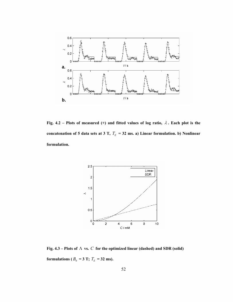
52

Fig. 4.2 – Plots of measured (+) and fitted values of log ratio, λ . Each plot is the

concatenation of 5 data sets at 3 T, ET = 32 ms. a) Linear formulation. b) Nonlinear

formulation.

Fig. 4.3 – Plots of Λ vs. C for the optimized linear (dashed) and SDR (solid)

formulations ( 0B = 3 T; ET = 32 ms).

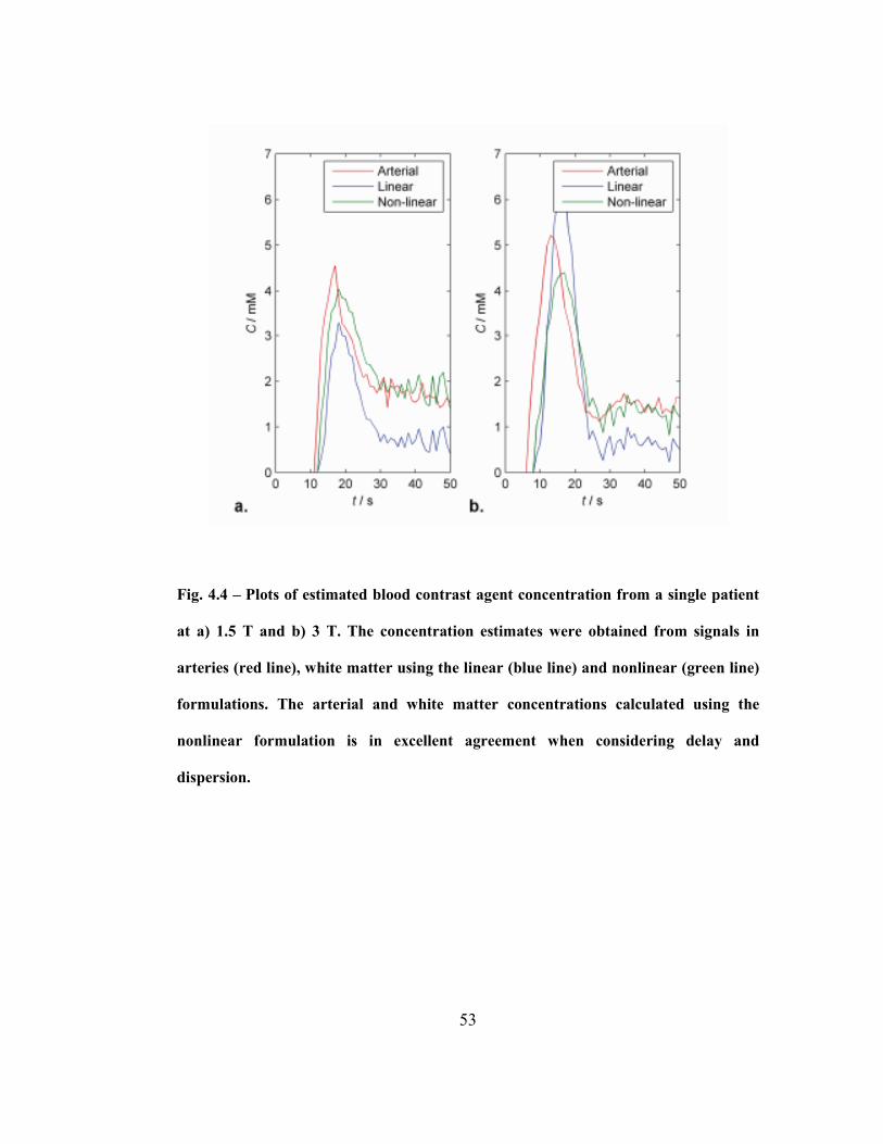
53

Fig. 4.4 – Plots of estimated blood contrast agent concentration from a single patient

at a) 1.5 T and b) 3 T. The concentration estimates were obtained from signals in

arteries (red line), white matter using the linear (blue line) and nonlinear (green line)

formulations. The arterial and white matter concentrations calculated using the

nonlinear formulation is in excellent agreement when considering delay and

dispersion.

54

Fig. 4.5 – Box and whisker plots of fractional error in ROI and single pixel

measurements in white matter (a and b) and grey matter (c and d) CBV estimates

obtained using the linear and nonlinear formulations at 1.5 T and 3 T. In each box,

the central line represents the median of measurements in five test patients, the upper

and lower boundaries of the box represent the upper and lower quartiles and the

whiskers represents the range.

55

Table 4.1 – Fractional error in white and grey matter CBV estimates (%) relative to

literature values by the linear and nonlinear equations at 1.5 and 3T for both ROI

and single voxel measurements.

1.5 T 3 T

ROI Voxel ROI Voxel

Linear -10.1% ± 18.8 17.2% ± 17.7 46.2% ± 9.4 45.1% ± 10.2

WM

Nonlinear 0.5% ± 3.1 6.5% ± 9.1 -0.3% ± 1.8 0.7% ± 6.9

Linear 40.7% ± 18.6 57.0% ± 23.6 123.9% ± 19.1 121.5% ± 20.0

GM

Nonlinear -1.1% ± 5.1 -1.6% ± 11.4 0.7% ± 1.8 -6.7% ± 5.5

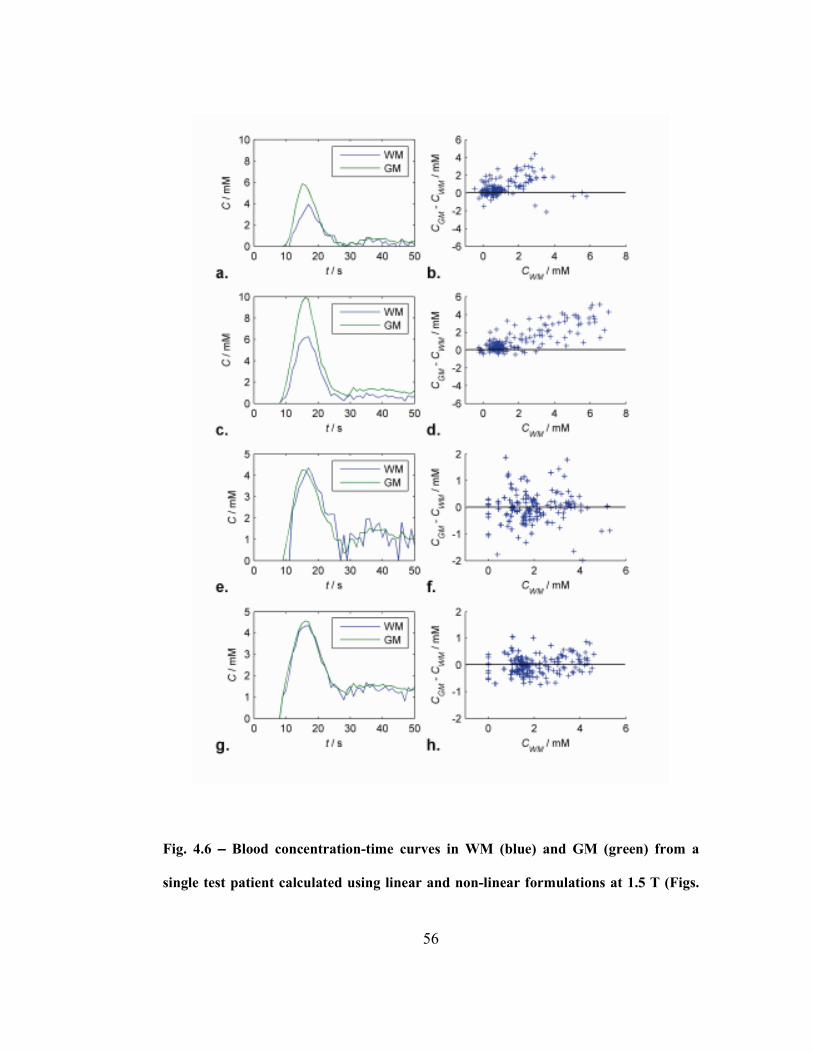
56

Fig. 4.6 – Blood concentration-time curves in WM (blue) and GM (green) from a

single test patient calculated using linear and non-linear formulations at 1.5 T (Figs.

57

4.6a and e) and 3 T (Figs. 4.6c and g), respectively. Differences between scaled GM

and WM curves from the beginning of the bolus to 30 seconds after are plotted

against WM concentration over all test patients at using linear and non-linear

formulations at 1.5 T (Fig. 4.6b and f) and 3 T (Fig. 4.6d and f), respectively.

Discussion

Estimating contrast agent concentration from changes in relaxation rate is

the essential first step in making contrast-based MRI perfusion measurements.

Without an accurate relationship, absolute quantification of perfusion parameters is

impossible. Furthermore, because relaxivity in tissues may be a complex function

of contrast agent concentration, field strength and echo time (i.e., it is not

necessarily a simple linear function), an accurate comparison of results between

sites using different imaging protocols is challenging. Although the theory of

relaxivity is quite well established it consists of a number of different regimes and

it is sometimes unclear which is applicable in practice. We believe that this study

represents the first attempt to compare different functional forms for relaxivity – a

linear approximation and a nonlinear interpolation formula – empirically.

It is clear from Figs. 4.2 and 4.3 that the linear approximation

underestimates high values of concentration and overestimates low values.

Difficulty in reconciling the over- and underestimates with the measured data will

contribute to the errors in accuracy seen in Fig. 4.5, and it seems likely may also

contribute to the poor precision. All patients underwent the same injection protocol,

58

if a different injection rate were used or if patients had variable cardiac output, we

would expect to see greater errors. Finally, the apparently systematic difference in

errors at 1.5 and 3 T suggest that a single linear relaxivity constant cannot

adequately describe relaxivity at different field strengths or echo times.

The results using the linear function suggest that the correct function should

have an increasing slope. That is relaxation rate must change relatively slowly with

concentration at low concentration and faster at high concentration. The nonlinear

formulation is therefore of the more appropriate form (Fig. 4.3) and gives excellent

agreement between: 1) experimental and fitted curves (Fig. 4.2); 2) arterial and

WM derived blood CTCs (Fig. 4.4) after considering dispersion; 3) CBV values for

WM and GM (Fig. 4.5); 4) WM and GM CTCs (Fig. 4.6). The agreement appears

equally good at the two field strengths and echo times suggesting that the

formulation should hold good for a variety of different imaging protocols.

The very low values of fractional error seen with the nonlinear model in

Fig. 4.5 are partially because the calibration method used here forces measured

values towards the assumed, literature value. (I.e., fractional error is relative to the

assumed value not to the true value which is unknown.) However, calibration

coefficients were derived from white matter measurements and then applied to grey

matter in test subjects. Agreement with literature values of grey matter (which had

not been used in the calibration) were nonetheless excellent. Furthermore, the same

calibration procedure was used to obtain optimum linear coefficients which still

produced an apparent bias in estimates, once again confirming that a linear model is

59

inadequate for describing relaxivity. The systematic overestimation of CBV at 3 T

relative to 1.5 T emphasizes the problems in finding a single linear relaxation

relationship that fits multiple field strengths. The bias in the linear results is due to

the inability of linear expression to adequately track the bolus portion of the curve

(Fig. 4.4).

Calibration values were calculated on the basis of PET literature values of

WM blood volume, the gold standard. The low fractional error in WM test

estimates relative to the same literature values seen in Fig. 4.5 might therefore be

expected. However, GM literature values were not used in the calibration

procedure, only in testing, and therefore cannot explain the low fractional error in

these estimates. Furthermore, the same literature values of WM were used to obtain

the linear calibration curves which nonetheless demonstrate large biases. Also, the

low variance of these estimates at both field strengths suggests that even if not

accurate they should at least be consistent across field strengths and echo times.

Note also, that although it is not often made explicit, the use of literature values of

brain blood volumes is universal. Since the relaxivity of contrast in brain

microvasculature is unknown, but much greater than that in arteries, it is necessary

to introduce a calibration factor to obtain realistic estimates of CBV.

The values for the coefficient b can be found theoretically using Eq. (4.7);

γ = 2.675·108

rad·s-1

T-1

, k = 0.027 ppm·mM-1

(80), b is 30 for isotropically

distributed vessels ( ( )4 3η π= (33)) and 45 for vessels perpendicular to the

60

external magnetic field ( 2η π= (81)). This compares quite well with the optimum

value of 28.9 found for the linear formulation, but is very far from the optimum of

114.4 found for the nonlinear formulation. There are number of possible

explanations for this. First, Hct and oxygen extraction fraction (OEF) levels vary

depending on age, gender and medical conditions and treatment. However,

although a rather large effect is seen in the empirical studies of whole blood

(53,55,82), it is much reduced when plasma concentration is considered. That is,

the relaxivity of X moles of CA per ml of plasma is very similar regardless of Hct

or OEF. Since our calibration procedure (Eq. (4.9)) takes Hct explicitly into

account, the effect on our results will be small. Second, the SDR formula is based

on modeling the vasculature as infinitely long straight cylinders, which is an

idealization that may introduce errors into theoretical estimates. However, it again

seems unlikely that these errors will be sufficient to explain the discrepancy. The

most likely explanation may lie in inaccuracies in the interpolation formula, Eq.

(4.8). Although the formula is reliable at low and high concentrations, and is of a

reasonable functional form, its accuracy is unknown at intermediate concentrations.

The slope of the linear asymptote of Eq. (4.6) may critically affect the curvature of

the interpolation section. Since the brain parenchyma concentrations on which our

calibration is based fall into this intermediate range, our results will be biased

towards finding good agreement in this range at the expense of accuracy at high

concentrations. Support for the hypothesis that the form of the interpolation

determines the empirical optimum of b is given by our finding that the alternative

61

interpolation formula of Kiselev (35) gives a very different optimum (~220, even

farther from the theoretical value). Better agreement may therefore be found with

alternative interpolation formulae. Nonetheless, the empirically optimum value of

b used with Eq. (4.8) gives excellent agreement over the range of concentrations

found in normal brain with standard doses of contrast. Furthermore, the success of

our calibration values in predicting grey matter CBV suggests applicability when

vascular density is moderately increased. However, these values should be used

with caution at very high values of C where the linear range applies. Moreover, in

areas where vessel density is greatly increased, the effects of diffusional narrowing

may begin to invalidate Eq. (4.6). Thus, oncological applications of this

methodology to highly vascularized neoplasms should be considered carefully and

quantitatively.

The close agreement between grey and white matter measurements seen in

Fig. 4.6 suggests that the static dephasing regime is adequate to describe relaxivity

in normal tissue and therefore that diffusional narrowing (83) is negligible in these

circumstances.

There are a number of limitations in this study. 1) We did not attempt to

measure Hct or OEF. 2) The empirically determined bulk blood relaxivity curves

used in this study were created using a different Gd chelating agent, Optimark

gadoversetamide (Gd-DTPA-BMEA), than that used in our study. However

calibration curves obtained at 1.5 T using different compounds show only small

differences. 3) We have considered only Gd contrast agents. Different calibration

62

values are likely to be found with other paramagnetic agents or superparamagnetic

agents (e.g., ultra-small, superparamagnetic iron oxide particles). 4) Our control

subjects at 1.5 T were meningioma patients. Although it would have been

preferable to use healthy subjects, it proved difficult to recruit subjects given

concerns over nephrogenic systemic fibrosis. However, meningiomas are extra-

axial tumors that do not infiltrate into normal brain, and there is no reason to

suppose they substantially alter the vasculature. This is confirmed by our finding

that CBV estimates in these patients agree with values obtained in controls at 3 T.

5) It would have been preferable to obtain our calibration values of WM blood

volume by direct measurements of our subjects using the gold standard of PET. We

cannot therefore claim that our results in Fig. 4.5 are accurate but merely consistent

with expected values. 6) Finally, this calibration was based on estimates of the

arterial input function. This is notoriously difficult to estimate due to partial volume

effects. To some extent the procedure presented here is self-correcting in that the

coefficients are chosen to give the expected, literature values. That is, if the area

under the AIF were reduced by a factor α, then the empirical coefficients r and b

would be increased by a similar factor to generate the expected CBV value. (Note,

however, that in the nonlinear case this would also produce distortions in the CTC.

That none are seen in Figs. 4.4 and 4.6 provides evidence that AIF partial volume

effects were small in this study.) Provided partial volume effects in our subjects

were typical, it should not affect the consistency across protocols (rather than

precision) of results obtained with these calibration values. Furthermore, the small

63

variance in measured results suggests that AIFs were, in practice, relatively

reproducible from patient to patient. This may be because we took particular care to

exclude pixels where “spiky” boluses or saturation suggested phase cancellation

due to partial volume effects.

In conclusion, we have derived a calibration curve that gives consistent

estimates of contrast agent concentration from measured relaxivity changes in

white matter and grey matter at different values of ET and 0B and which should be

applicable in a wide range of conditions. The function has the same functional form

as the nonlinear interpolation formula of Yablonskiy and Haacke (Eq. (4.8)) with

ω = 114.4 0CB . Linear approximations are not adequate to describe relaxivity in

brain parenchyma. To our knowledge, this study represents the first attempt to

confirm any theoretical form of *

2T relaxivity in tissue experimentally and the first

to provide a reliable expression for relaxivity in the brain.

64

CHAPTER 5: *

2R∆ Relaxivity in Venous Blood

The work in this chapter appears in Magnetic Resonance in Medicine under the

following citation:

Patil V, Johnson G. DeltaR2 (*) gadolinium-diethylenetriaminepentacetic acid

relaxivity in venous blood. Magn Reson Med 2013;69(4):1104-1108.

This study was funded in part by NIH grant RO1CA111996.

Author Contributions:

Vishal Patil – Project concept and design, data acquisition and analysis,

manuscript drafting and revisions.

Glyn Johnson – Project concept and design, manuscript drafting and

revisions, final approval for publication.

65

Abstract

The accuracy of perfusion measurements using dynamic susceptibility

contrast (DSC) MRI depends on estimating contrast agent concentration in an

artery, i.e., the arterial input function (AIF). One of the difficulties associated with

obtaining an AIF are partial volume effects (PVEs) when both blood and brain

parenchyma occupy the same pixel. Previous studies have attempted to correct

AIFs which suffer from PVEs using contrast concentration in venous blood.

However, the relationship between relaxation and concentration (C ) in venous

blood has not been determined in vivo. In this chapter a previously employed fitting

approach is used to determine venous relaxivity in vivo. In vivo relaxivity is

compared to venous relaxivity measured in vitro in bulk blood. The results show

that the fitting approach produces relaxivity calibration curves which give excellent

agreement with arterial measurements.

66

Introduction

Measurements of venous concentration can be used to automate arterial

pixel selection and correct for partial volume effects in the arterial input function

(AIF, i.e., the concentration of tracer in arteries) (84-86). These methods have

assumed that the relaxivity of arterial and venous blood are the same. However, this

is not generally the case as the presence of paramagnetic deoxyhemoglobin in will

contribute to venous relaxivity. A recent study by Blockley et al. empirically

determined the relaxivity of venous blood in vitro at different field strengths using

a blood phantom doped with a Gd based tracer (56). This study found that

relaxivity was quadratic with the minimum at some positive value of Gd

concentration, C . I.e., that relaxivity initially decreases with increasing C , as the

presence of paramagnetic Gd decreases field differences between diamagnetic

plasma and paramagnetic deoxygenated red blood cells. This would result in an

increase in signal intensity at the beginning of the bolus but this behavior does not

appear to be observable in vivo.

The aim of this note is therefore to determine the relaxivity of venous blood

by a fitting approach previously used in Ch. 4 to determine brain parenchyma

relaxivity (87). The approach determines the quadratic venous relaxivity function

that gives the best agreement between the areas under arterial and venous

concentration-time curves (CTCs).

67

Methods

The study was approved by the Institutional Review Board of this

institution. DSC data was acquired from 6 meningioma subjects at 1.5 T ( RT = 1 s;

ET = 47 ms; FA = 40°; matrix 128 × 128; FOV 228 × 228 mm2; 7 × 5 mm slices)

and 3 T ( RT = 1 s; ET = 32ms; FA = 30°; matrix 128 × 128; FOV 230 × 230 mm2;

10 × 5 mm slices) using a gradient echo EPI sequence during injection of 0.1

mmol/kg Gd-DTPA.

Arterial and venous pixels are detected semi-automatically using

adaptations of techniques first suggested by Rempp et al. (36). First, signal was

averaged over all images at each time point to obtain an average brain signal.

Although it might be preferable to extract the brain first, in practice this average is

dominated by brain pixels. The following parameters are then measured: fractional

signal drop (FSD), full width at half drop (FWHD) and arrival time (AT, defined as

the time at which signal is decreased by 10% of the maximum FSD). Candidate

arterial pixels were defined as those with a FWHD at least 1 s less than the average

brain value and an AT at least 1 s before the average brain value. Similarly

candidate venous pixels were defined as those 1s wider and 1s later than the

average. Candidate pixels were visually inspected and the ten with the greatest FSD

that showed no evidence of signal saturation, “spiky” boluses, indicative of phase

cancellation with surrounding parenchymal pixels (54) were averaged to produce

arterial and venous measurements for each patient.

68

Signal intensity in a *

2T -weighted EPI acquisition (neglecting T1 effects) is

given by

( ) ( )( )exp 0preS S C= Λ − Λ (5.1)

where preS is the pre-bolus signal and Λ is a function of concentration. The

relaxivity of arterial bulk blood has been measured empirically at multiple field

strengths and has been found to follow a quadratic form:

( ) ( )2

EC qC pC TΛ = + . (5.2)

At 1.5 T, q = 0.74 s-1

mM-2

and p = 7.62 s-1

mM-1

(71); at 3 T, q = 2.61 s-1

mM-2

and p = 0.5 s-1

mM-1

(53). (Hematocrit was 40% in both cases.)

The in vitro relaxivity of venous bulk blood with a 30% oxygen extraction

fraction (OEF) follows a parabola but with a shift (a ) along the concentration axis

( ) ( )( )2

EC q C a pC TΛ = − + . (5.3)

At 1.5T, q = 6 s-1

mM-2

, p = -11 s-1

mM-1

and a = -0.046 mM; 3T, q = 18 s-1

mM-

2, p = -35 s

-1mM

-1 and a = 0.037 mM (hematocrit 42%) (56).

In this study we assumed the same form for relaxivity as found in bulk

blood, Eq. [3], but found the parameters q , p and a that gave the best agreement

between arterial and venous CTCs by the following fitting procedure similar to that

used previously used to determine parenchymal relaxivity (87).

69

All CTCs were fitted to the SCR model (Eq. (3.2) (79). The SCR model is

preferable to the alternative of fitting a gamma variate to the bolus portion of the

CTC alone for a number of reasons.

The procedure is based on the basic postulates of DSC MRI that 1) the area

under the bolus (Eq. (3.4)), A , must be equal for arterial and venous (and all other

vascular) CTCs and 2) the height of the recirculation portion of the CTCs must also

be equal. The values of q , p and a that best realize these conditions were found

by simultaneously fitting CTCs from 5 patients at both 1.5 and 3 T. Briefly, for

each patient, A and κ are estimated in the artery by modeling the CTC as Eq.

(3.2), converting to signal using Eq. (5.1) and the bulk arterial blood relaxivity

curves (Eq. (5.2)) and fitting to the measured signal with preS , maxy , 0t , maxt , α

and κ as free parameters. Similarly each vascular CTC is modeled by Eq. (3.2),

converted to signal using Eqs. (5.1) and (5.3) and fitted to the measured signal.

However, the venous fit is constrained to give equal values of A and κ to those

found in the artery but with the relaxivity parameters q , p and a as fitting

parameters in addition to preS , 0t , maxt and α . Fits to all 5 patients were performed

simultaneously with different gamma variate parameters for each patient but the

same relaxivity parameters for all. Since we are comparing two pools of blood with

the same hematocrit, it is not necessary to correct for this. Fitting to signal rather

than estimates of concentration avoids errors associated with the nonlinear

70

relationship between noise and concentration (55,88). Including preS as a fitting

parameter is somewhat unusual but should provide the best overall fit of the data.

Results

Fig. 5.1 shows measured (points) and fitted (line) venous signal

measurements for 5 patients at 1.5 (a) and 3 T (b). Table 5.1 gives the coefficients

for venous relaxivity (Eq. (5.3)) derived from in vivo fitting. It should be noted the

a term is very small and can in practice be neglected. This finding is in contrast to

that in in vitro bulk blood (56) measurements. Fig. 5.2 shows relaxivity calibration

curves for arterial (red) blood, in vitro bulk venous blood (56) (black; coefficients

are given in the methods section) and in vivo venous blood (blue) at 1.5 (a) and 3 T

(b).

Fig. 5.3 shows CTCs derived for arterial signals (red), and venous signals

using in vitro bulk blood relaxivity (black) and in vivo venous relaxivity

expressions (blue) at 1.5 (a) and 3 T (b). (The discontinuities in the in vitro curves

are due to the ambiguity in relaxivity estimation caused by the non-mononotic

nature of the in vitro relaxivity curve. Values between zero concentration and the

first non-ambiguous concentration have therefore been derived by interpolation.)

With the in vivo relaxivity, the relative widths, heights and arrival times of the

arterial and venous curves are consistent with what would be expected from delay

and dispersion: the arterial bolus starts before and is narrower and higher than the

venous, the recirculation portion of the curve is of similar height. The venous CTC

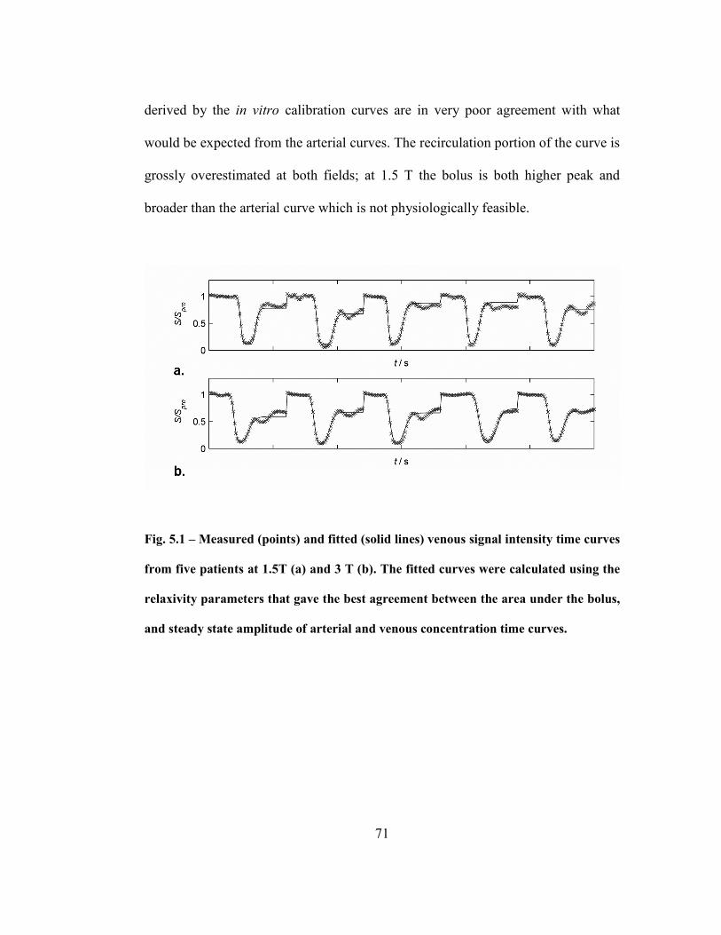
71

derived by the in vitro calibration curves are in very poor agreement with what

would be expected from the arterial curves. The recirculation portion of the curve is

grossly overestimated at both fields; at 1.5 T the bolus is both higher peak and

broader than the arterial curve which is not physiologically feasible.

Fig. 5.1 – Measured (points) and fitted (solid lines) venous signal intensity time curves

from five patients at 1.5T (a) and 3 T (b). The fitted curves were calculated using the

relaxivity parameters that gave the best agreement between the area under the bolus,

and steady state amplitude of arterial and venous concentration time curves.

72

Table 5.1 – Relaxivity coefficients for Eq. (5.3) (curves shown in Fig. 5.2).

q p a

1.5 T 0.74 7.62 0

Arterial

3 T 2.61 0.5 0

1.5 T 0.0018 19.0 0.0086

In vivo fitting

3 T 0.74 12.1 0.0095

1.5 T 6 -11 -0.046

In vitro bulk blood

3 T 18 -35 0.037

Fig. 5.2 – Arterial (red) and venous (in vitro – black; in vivo – blue) relaxivity

calibration curves at 1.5 T (a) and 3 T (b). Curve coefficients are given in Table 5.1.

73

Fig. 5.3 – Arterial and venous CTCs at 1.5T (a) and 3T (b). The discontinuities in the

in vitro venous curves are because the same value of *

2R∆ corresponds to two different

concentrations below about 2 mM (see Fig. 5.2). The curve was therefore obtained by

interpolation between zero and the first unambiguous value of *

2R∆ .

Discussion

Theoretical modeling of Gd relaxivity in blood is a difficult problem and, as

far as we are aware, has not yet proved amenable to analysis. Relaxivity

expressions have therefore been found empirically using phantoms and been shown

to resemble a quadratic for both arterial and venous blood. In this study we

therefore empirically determined the quadratic function that best describes

relaxivity in in vivo venous blood at 1.5 and 3 T. The excellent fits in Fig. 5.1

confirm that quadratic functions adequately describe venous relaxivity although

74

they do not prove that this is the true functional form. The agreement between

arterial and venous CTCs derived from the in vivo relaxivity expressions (Fig. 5.3)

further confirm this.

The quadratic term in the 1.5 T in vivo relaxivity expression is very small,

unlike that in other measurements. Again, theoretical modeling is difficult and we

have no good explanation for this finding. However, we do note that similar

findings are seen in arterial measurements.

The in vitro relaxivity curves (Fig. 5.2) give negative *

2R∆ over a critical

range of concentrations that include those seen during recirculation (between 0.5

and 1 mM – Fig. 5.3). If the arterially derived concentrations are correct the in vitro

curves would predict a distinct signal increase at the beginning of the bolus and a

recirculation portion greater than preS . Neither of these are seen in any venous

measurements (Fig. 5.1).

Relaxivity is largely determined by magnetic field inhomogeneities caused

by susceptibility differences between diamagnetic plasma, paramagnetic

deoxyhemoglobin confined to the red blood cells (RBCs), paramagnetic contrast

agent within the plasma and the diamagnetic surroundings (tissue in vivo, air or

water in vitro). In large phantoms, inhomogeneities will be dominated by

differences between plasma and RBCs. As the concentration of contrast agent

increases these inhomogeneities will initially decrease until the susceptibility of the

plasma equals that of the RBCs, creating a minimum in the relaxivity curve shifted

to the right along the concentration axis. In small vessels, however, susceptibility

75

differences between the lumen and surrounding tissue will also contribute to

inhomogeneity and hence relaxivity. The initial dose of contrast agent will increase

these inhomogeneities thus potentially negating the effect of RBC/plasma

differences. This could explain the discrepancy between in vitro and in vivo

relaxivities. If this explanation is correct it suggests that the relaxivity parameters

derived here will be somewhat dependent on vascular diameter and should

therefore be used with caution in veins different in size from cerebral veins. (Note

that this effect would have less effect on in vitro measurements of arterial blood

since oxygenated RBCs are diamagnetic.)

There a number of limitations to this study: First, DSC data must be

acquired with sufficient temporal resolution to capture the passage of the bolus so

relatively low spatial resolution acquisitions are employed. Blood vessels are

therefore likely to be smaller than the dimensions of pixels so that vascular

measurements are contaminated by partial volume effects (PVEs). This study is

partially resistant to errors from simple PVEs where the bolus is reduced in

amplitude without distortion since the calibration procedure uses the relative size of

different portions of the CTC (by constraining κ ) (38). However, PVEs can also

result in phase cancellation of signal between vessels and surrounding tissue

(54,89). Such phase errors can introduce distortions in bolus shape and errors into

the calibration. These errors also usually cause characteristically “spiky” and

square signal drops that approach zero. For this reason we visually inspected the

candidate arterial and venous curves and rejected those showing these effects.

76

Although this procedure is not certain, the consistent fits achieved (Fig. 5.1)

suggest that any residual effects are relatively small. Second, hematocrit and OEF

will influence relaxivity (55) so that large variations in these parameters will reduce

the accuracy of our calibration values. However, a previous study by Akbudak et al.

demonstrates that provided plasma concentrations are compared, hematocrits

between 30% and 40% do not produce large differences in *

2R within the range of

concentration in which we are interested (0-5 mM) (53). Thirdly, the in vitro

experiments used ProHance as a gadolinium chelate, not Gd-DTPA. This may

explain some of the discrepancies though there appears to be little evidence in the

literature to suggest major relaxivity differences between most contrast agents.

Lastly, the in vitro relaxivity curve was determined over a smaller range of

concentrations than the in vivo so that the latter may be more reliable at high

concentrations.

77

CHAPTER 6: Perfusion in Normal Appearing White Matter in

Glioma Patients Treated with Bevacizumab: A Clinical Study

The work in this chapter is undergoing review in a peer-reviewed journal and

appears in Proceedings of ISMRM 20th Annual Meeting, Melbourne, Australia

under the following citation:

Patil V., Johnson G., Reductions in blood volume in normal white matter are found

in glioma patients treated with bevacizumab. Proceedings of ISMRM 20th

Annual Meeting, Melbourne, Australia, 2012.

This study was funded in part by NIH grant RO1CA093992.

Author Contributions:

Vishal Patil – Project concept and design, data acquisition and analysis.

Manu Singh – Data analysis.

Maya Mathew – Data acquisition.

Ashwathan Narayana – Project concept and design.

James Babb – Data analysis.

David Zagzag – Project concept and design.

Glyn Johnson – Project concept and design, manuscript drafting and

revisions.

78

Abstract

We previously made the incidental observation that MRI estimates of

cerebral blood volume (CBV) were reduced in the contralateral white matter (WM)

of glioma patients treated with bevacizumab. The purpose of the study was

therefore to investigate changes in MRI perfusion measurements that accompany

treatment with bevacizumab. Dynamic, susceptibility-weighted, contrast-enhanced

(DSC) MRI was performed on three groups of glioma patients: Group I. Newly

diagnosed patients treated without bevacizumab. Group II. Newly diagnosed

patients receiving bevacizumab. Group III. Patients receiving bevacizumab on

recurrence. Serial post-treatment scans were performed in all groups. Serial pre-

treatment scans were available for Group III. Estimates of CBV and cerebral blood

flow (CBF) were obtained in contralateral white and grey matter (GM) from all

scans. Statistically significant reductions in CBV were seen in WM and GM in

Groups II (p < 0.01) and III (p < 0.0001). CBF was reduced in WM in Group II and

WM and GM in groups II and III (p < 0.05). No significant changes were seen in

group I. Post-treatment rates of change CBV were negative in WM and GM (p <

0.01) in Groups II and III. No significant rate of change of CBV was found in

group I or in the pre-treatment measurements of Group III. No significant rate of

change was found in CBF in either tissue in any group. Reductions in CBV and

CBF are seen in normal appearing contralateral brain tissue in glioma patients

treated with bevacizumab. CBV reductions increase with time even after treatment

has ended.

79

Introduction

Bevacizumab (Avastin®, Genentech, San Francisco, CA) was the first FDA

approved anti-angiogenic agent and has shown efficacy in a number of different

tumors including glioma when used in combination with conventional cytotoxic

agents (90,91). We have recently been investigating the use of perfusion

measurements obtained by dynamic, susceptibility-weighted, contrast-enhanced

(DSC) MRI in assessing response in glioma patients treated with bevacizumab.

During the course of this investigation we made the incidental observation that

blood volumes in normal appearing white matter (NAWM) appeared reduced in

these patients. In this study we therefore investigated whether this observation

could be confirmed and whether it was associated specifically with bevacizumab

treatment.

Methods

This retrospective study was approved by the Institutional Review Board of

this institution. DSC MRI scans 1.5 T were: ( 0B = 1.5 T; ET = 40-47 ms, RT =

1000 ms; field of view, 228×228 mm2; 10 slices; section thickness, 5 mm; matrix,

128×128; in-plane voxel size, 1.78×1.78 mm

2; FA = 40-90°) were acquired using a

gradient echo EPI sequence during injection of 0.1 mmol/kg Gd-DTPA from three

groups of patients: Group I received a combination of radiotherapy and

chemotherapy but no bevacizumab at initial diagnosis. Group II received

bevacizumab and temozolomide after surgery and radiotherapy following initial

80

diagnosis. Group III received bevacizumab and irinotecan after tumor recurrence,

having previously received radio- and chemotherapy without bevacizumab at initial

diagnosis. Most patients underwent resection at initial diagnosis. Newly diagnosed

patients were scanned immediately before treatment and at 2-3 month intervals

thereafter. Recurrent glioma patients were scanned at 2-3 month intervals between

initial diagnosis and recurrence and at similar intervals subsequently.

Absolute cerebral blood volume (CBV), cerebral blood flow (CBF) and

mean transit time (MTT) were calculated using standard methods that will be

summarized here. Tracer concentration is first calculated from the measured signal

change using empirically derived calibration curves (59). Total tissue concentration

of tracer, tC , is given by the expression:

( ) ( ) ( )CBFt aC t R t C t= ⋅ ⊗ (6.1)

where ( )R t is the tissue residue function, i.e., the fraction of tracer arriving in the

tissue at time zero that remains at time t , aC is the concentration in the artery

feeding the tissue ⊗ represents convolution and we have neglected terms related to

tissue density and hematocrit. Since ( )0R equals one by definition, estimates of

CBF can be obtained by deconvolving tC by aC . This was achieved using block-

circulant singular value decomposition (40,42) with Tikonov regularization (44).

Other parameters are calculated from the following expressions (32):

( )0

MTT R t dt

∞

= ∫ (6.2)

81

and

CBV CBF MTT= ⋅ (6.3)

aC was measured using a semiautomatic approach adapted from techniques first

suggested by Rempp et al. (36).

Signal time curves were measured in normal appearing grey and white

matter in the caudate nucleus and frontal lobes contralateral to the tumor. CBV,

CBF and MTT were calculated for these ROIs as described above. Measurements

were made both before and after treatment. Most patients had multiple post-

treatment measurements between 2 and 120 months after treatment. Most recurrent

glioma patients (Group III) had multiple measurements both before and after

treatment.

The change in each perfusion parameter between the last pre-treatment and

first post-treatment scan was assessed using a paired sample t test. Where multiple

pre- (Group III) or post-treatment measurements (all groups) were available the rate

of change (i.e., slope vs. time) of each parameter was assessed by mixed model

regression. The analysis was stratified by measure, tissue type (grey or white

matter) and epoch (before vs. after treatment). In each case, the perfusion measures

at all pertinent available time points constituted the dependent variable and the

model included elapsed time from baseline (in months) as a fixed numeric factor

and subject ID as a random classification factor (to account for inter-subject

differences in mean perfusion levels and to account for the correlation among

82

measures from the same subject). Statistical tests were conducted at the two-sided

5% comparison-wise significance level using SAS 9.3 (SAS Institute, Cary, NC).

Results

Table 6.1 summarizes the demographics and histological diagnoses of the

different patient groups.

Fig. 6.1 and Table 6.2 the value of each perfusion measure at the last time

point before treatment and the first time point after treatment for each group. No

statistically significant changes were seen in any perfusion parameter in the group

that did not receive bevacizumab (Group I). CBF fell by between 19% and 25% in

all tissues in the two groups that did receive bevacizumab (Groups II and III). All

changes but that in GM in Group II were statistically significant (p = 0.04 or less;

values are given in Table 6.2). CBV fell by between 9% and 15% in all tissues in

both groups treated with bevacizumab (p = 0.002 or less). All changes were

statistically significant. No statistically significant changes were seen in MTT

values.

Fig. 6.2 and Table 6.3 give the rates of change of each perfusion measure

before and after treatment. No rate of change of any parameter in any pre-treatment

groups was significantly different from zero i.e., all pre-treatment parameters were

constant to within the measurement precision. However, in both groups treated with

bevacizumab (Groups II and III) CBV fell significantly in both GM and WM in the

83

months after treatment. No other statistically significant rates of change were

observed.

Table 6.1 – Patient demographics for each group.

Group N M/F Age Median (range) Grade (II/III/IV)

I 8 7/1 59 (41-77) 0/5/3

II 10 8/2 56 (33-75) 0/3/10

III 24 15/9 42 (12-78) 2/8/14

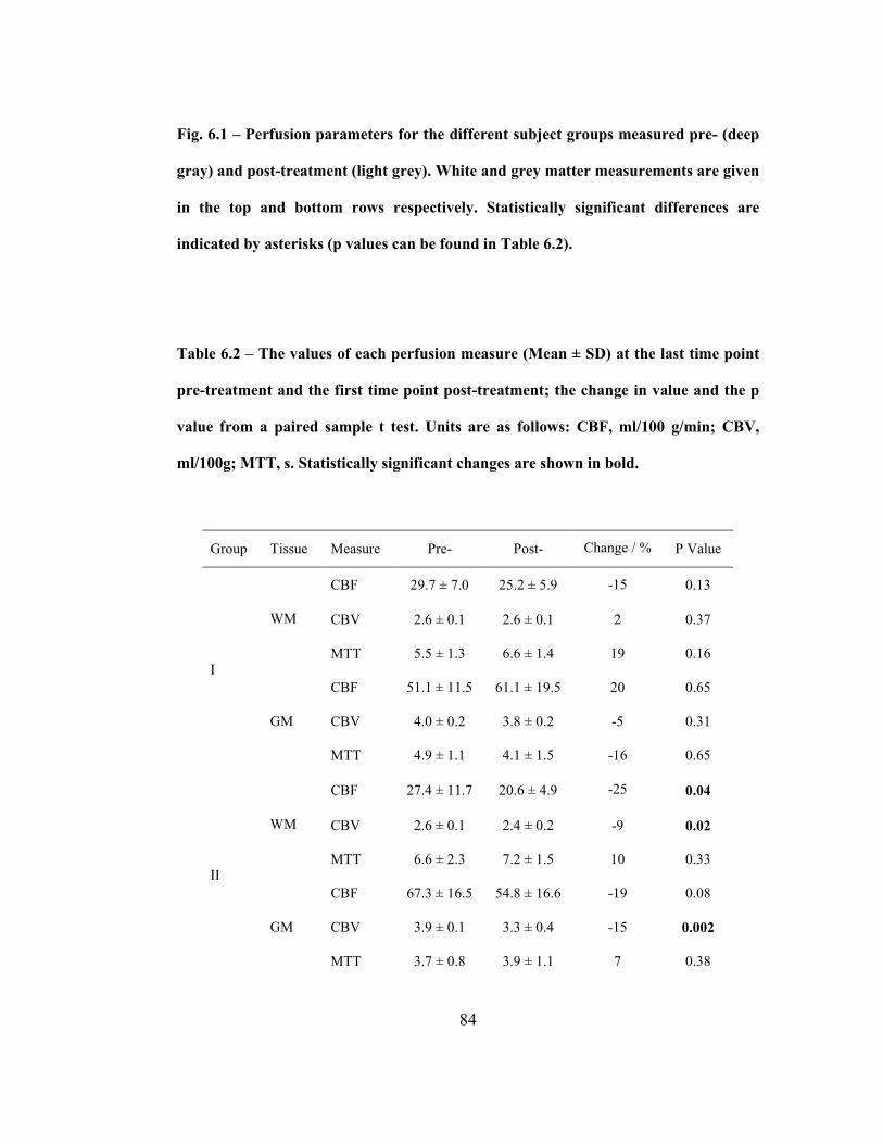
84

Fig. 6.1 – Perfusion parameters for the different subject groups measured pre- (deep

gray) and post-treatment (light grey). White and grey matter measurements are given

in the top and bottom rows respectively. Statistically significant differences are

indicated by asterisks (p values can be found in Table 6.2).

Table 6.2 – The values of each perfusion measure (Mean ± SD) at the last time point

pre-treatment and the first time point post-treatment; the change in value and the p

value from a paired sample t test. Units are as follows: CBF, ml/100 g/min; CBV,

ml/100g; MTT, s. Statistically significant changes are shown in bold.

Group Tissue Measure Pre- Post- Change / % P Value

CBF 29.7 ± 7.0 25.2 ± 5.9 -15 0.13

CBV 2.6 ± 0.1 2.6 ± 0.1 2 0.37 WM

MTT 5.5 ± 1.3 6.6 ± 1.4 19 0.16

CBF 51.1 ± 11.5 61.1 ± 19.5 20 0.65

CBV 4.0 ± 0.2 3.8 ± 0.2 -5 0.31

I

GM

MTT 4.9 ± 1.1 4.1 ± 1.5 -16 0.65

CBF 27.4 ± 11.7 20.6 ± 4.9 -25 0.04

CBV 2.6 ± 0.1 2.4 ± 0.2 -9 0.02 WM

MTT 6.6 ± 2.3 7.2 ± 1.5 10 0.33

CBF 67.3 ± 16.5 54.8 ± 16.6 -19 0.08

CBV 3.9 ± 0.1 3.3 ± 0.4 -15 0.002

II

GM

MTT 3.7 ± 0.8 3.9 ± 1.1 7 0.38

85

CBF 26.9± 8.4 20.3 ± 5.5 -24 0.006

CBV 2.6 ± 0.2 2.3 ± 0.3 -15 0.0001 WM

MTT 6.3 ± 1.5 7.2 ± 1.5 14 0.07

CBF 65.4 ± 15.3 51.9 ± 14.9 -21 0.0008

CBV 3.9 ± 0.2 3.3 ± 0.4 -15 < 0.0001

III

GM

MTT 3.8 ± 0.9 4.2 ± 1.4 10 0.15

Fig. 6.2 – Fractional rates of change of each parameter per month (i.e., the vertical

scale is in units of month-1

) for CBF (left), CBV (middle) and MTT (right) for white

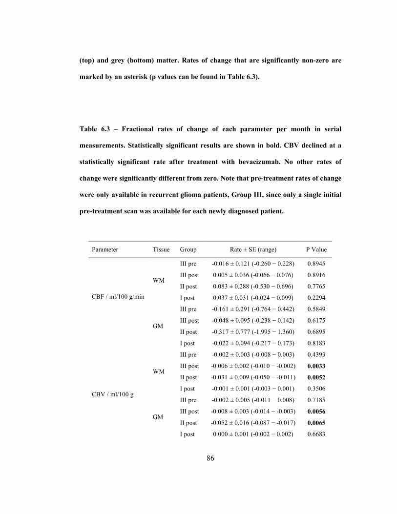
86

(top) and grey (bottom) matter. Rates of change that are significantly non-zero are

marked by an asterisk (p values can be found in Table 6.3).

Table 6.3 – Fractional rates of change of each parameter per month in serial

measurements. Statistically significant results are shown in bold. CBV declined at a

statistically significant rate after treatment with bevacizumab. No other rates of

change were significantly different from zero. Note that pre-treatment rates of change

were only available in recurrent glioma patients, Group III, since only a single initial

pre-treatment scan was available for each newly diagnosed patient.

Parameter Tissue Group Rate ± SE (range) P Value

III pre -0.016 ± 0.121 (-0.260 − 0.228) 0.8945

III post 0.005 ± 0.036 (-0.066 − 0.076) 0.8916

II post 0.083 ± 0.288 (-0.530 − 0.696) 0.7765 WM

I post 0.037 ± 0.031 (-0.024 − 0.099) 0.2294

III pre -0.161 ± 0.291 (-0.764 − 0.442) 0.5849

III post -0.048 ± 0.095 (-0.238 − 0.142) 0.6175

II post -0.317 ± 0.777 (-1.995 − 1.360) 0.6895

CBF / ml/100 g/min

GM

I post -0.022 ± 0.094 (-0.217 − 0.173) 0.8183

III pre -0.002 ± 0.003 (-0.008 − 0.003) 0.4393

III post -0.006 ± 0.002 (-0.010 − -0.002) 0.0033

II post -0.031 ± 0.009 (-0.050 − -0.011) 0.0052 WM

I post -0.001 ± 0.001 (-0.003 − 0.001) 0.3506

III pre -0.002 ± 0.005 (-0.011 − 0.008) 0.7185

III post -0.008 ± 0.003 (-0.014 − -0.003) 0.0056

II post -0.052 ± 0.016 (-0.087 − -0.017) 0.0065

CBV / ml/100 g

GM

I post 0.000 ± 0.001 (-0.002 − 0.002) 0.6683

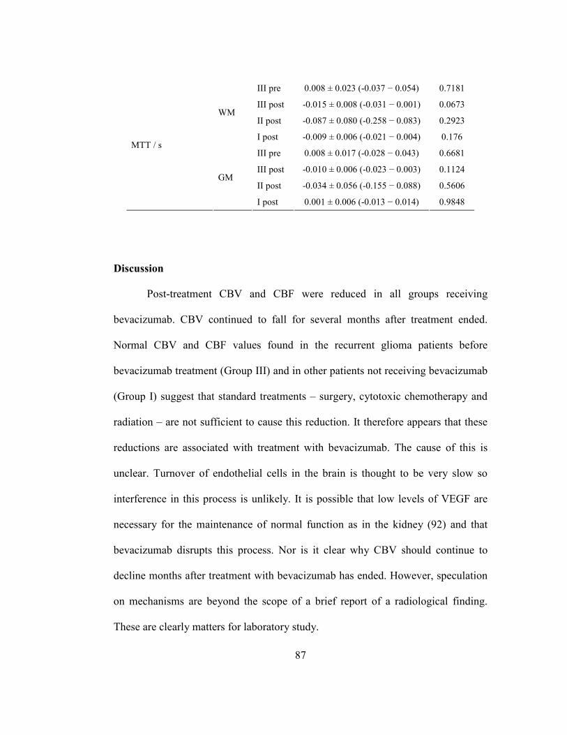
87

III pre 0.008 ± 0.023 (-0.037 − 0.054) 0.7181

III post -0.015 ± 0.008 (-0.031 − 0.001) 0.0673

II post -0.087 ± 0.080 (-0.258 − 0.083) 0.2923 WM

I post -0.009 ± 0.006 (-0.021 − 0.004) 0.176

III pre 0.008 ± 0.017 (-0.028 − 0.043) 0.6681

III post -0.010 ± 0.006 (-0.023 − 0.003) 0.1124

II post -0.034 ± 0.056 (-0.155 − 0.088) 0.5606

MTT / s

GM

I post 0.001 ± 0.006 (-0.013 − 0.014) 0.9848

Discussion

Post-treatment CBV and CBF were reduced in all groups receiving

bevacizumab. CBV continued to fall for several months after treatment ended.

Normal CBV and CBF values found in the recurrent glioma patients before

bevacizumab treatment (Group III) and in other patients not receiving bevacizumab

(Group I) suggest that standard treatments – surgery, cytotoxic chemotherapy and

radiation – are not sufficient to cause this reduction. It therefore appears that these

reductions are associated with treatment with bevacizumab. The cause of this is

unclear. Turnover of endothelial cells in the brain is thought to be very slow so

interference in this process is unlikely. It is possible that low levels of VEGF are

necessary for the maintenance of normal function as in the kidney (92) and that

bevacizumab disrupts this process. Nor is it clear why CBV should continue to

decline months after treatment with bevacizumab has ended. However, speculation

on mechanisms are beyond the scope of a brief report of a radiological finding.

These are clearly matters for laboratory study.

88

No changes were seen in MTT suggesting that the reductions in blood flow

directly reflect changes in volume and that there is no compensatory increase in

blood velocity.

The introduction of anti-angiogenic therapy to the conventional treatment

regimen for both newly diagnosed and recurrent HGG has shown a marked

radiologic response of 50-80% with an improvement in quality of life secondary to

the anti-edema effect (93,94). However, the increase in overall survival in glioma

has been only moderate, of about 3 months. After VEGF blockade with

bevacizumab, there has been a shift toward diffuse invasive relapse as a function of

an especially hypoxic microenvironment, increasing the expression of factors that

promote invasion (91,95-98). The relative absence of contrast-enhancing tumor

compared with the non-contrast enhancing phenotype in many of the patients might

serve to underscore the effect bevacizumab has on reducing vessel leakiness and

thereby preventing contrast from entering areas with tumor as well as promoting

tumor invasion. As a result, there is intense interest in imaging modalities like

perfusion studies to help in predicting the response to therapy. This study suggests

that care need be exercised in the use of relative CBV measurements (which use a

reference in normal WM) to monitor treatment with bevacizumab and possibly

other anti-angiogenic agents. Tumor relative CBV measurements are likely to

underestimate initial reductions in blood volume after bevacizumab treatment.

Furthermore the continued reduction in CBV in NAWM may suggest an apparent

increase in blood volume in stable tumors.

89

There are several limitations to this study. First, there were small variations

in imaging protocol across the subject group, in particular in flip angle. However,

this will only have a large effect when contrast agent extravasation reduces 1T

significantly (99). Since measurements were made in NAWM where the blood

brain barrier is intact we do not expect to see any major effects. Furthermore, there

appeared to be no systematic association between a particular protocol and patient

group so that any effects would appear as random noise rather than a systematic

bias. Moreover, this limitation did not apply in Group III where only scans that

used identical flip angles were analyzed.

Second, numbers of subjects, particularly in Groups I and II were small.

However, the consistency of the results from these groups with the larger Group III,

and the high statistical significance of, in particular, the CBV results give us

confidence that the measurements are broadly correct. The heterogeneity of tumor

grade within our patient group might also be seen as a limitation. However, if this

effect were somehow dependent on grade, then this confounding factor would tend

to reduce statistical significance rather than produce a false positive.

90

CHAPTER 7: Estimating Contrast Agent Concentration with

Magnetic Field Correlation Imaging: A Future Direction

The work in this chapter appears in Magnetic Resonance in Medicine under the

following citation:

Patil V, Johnson G, Jensen JH. Robust quantification of contrast agent (CA)

concentration with magnetic field correlation (MFC) imaging. Magn Reson

Med 2009;62(4):1002-1006.

This study was funded in part by NIH grants RO1CA093992 and RO1CA093992.

Author Contributions:

Vishal Patil – Project concept and design, data acquisition and analysis,

manuscript drafting and revisions.

Glyn Johnson – Project concept and design, data acquisition, manuscript

drafting and revisions.

Jens H. Jensen – Project concept and design, data acquisition, manuscript

drafting and revisions, final approval for publication.

91

Abstract

Contrast-enhanced perfusion studies of the brain by means of magnetic

resonance imaging (MRI) are used to estimate a number of important brain tissue

parameters, including cerebral blood flow and volume. In order to calculate these

parameters, the contrast agent (CA) concentration must first be estimated. This is

usually accomplished by measurement of a nuclear magnetic resonance (NMR)

relaxation rate with the assumption of a linear relationship between the rate and the

CA concentration. However, such a linear relationship does not necessarily hold in

biological tissues due to compartmentalization of the CA in either the intravascular

or extracellular spaces. Here we propose an alternative MRI method of CA

quantification based on measurement of the magnetic field correlation (MFC),

which is theoretically predicted to have a robust quadratic dependence on the CA

concentration even when the CA is compartmentalized. In this study, CA

concentration estimation by means of MFC is shown to be more accurate than

established methods based on relaxation rates in yeast cell suspensions.

92

Introduction

Estimation of contrast agent (CA) concentration, C , is an essential first step

in the measurement, of a number of different brain tissue parameters, such as

cerebral blood flow, cerebral blood volume and vascular transfer constant by

contrast enhanced perfusion MRI. To accomplish this, a linear relationship between

C and the change in relaxation rate due to the presence of CA is usually assumed,

i.e.

tissueR R rC= + (7.1)

where R is the relaxation rate ( 1R , 2R , or *

2R ), tissueR is the relaxation rate in the

absence of CA and r is a constant expressing the relaxivity of CA (which in

general is tissue dependent). However, it is known that this linear relationship is

only strictly valid for simple solutions and may not hold in tissues due to

compartmentalization of the CA in either the intravascular or extracellular spaces

(35,51). As a consequence, the application of Eq. (7.1) to the analysis of contrast

enhanced perfusion MRI data can lead to systematic quantification errors.

Another CA sensitive parameter is the magnetic field correlation (MFC),

which may also be estimated with MRI (100,101). The MFC is defined by

( ) 2

2 1 1 2MFC ( ) ( )t t B t B tγ δ δ− = (7.2)

where )(tBδ is the local magnetic field shift (relative to the uniform background

field) experienced by a water proton at a time t and γ is the proton gyromagnetic

ratio. That the MFC is a function of the time difference, 12 tt − , rather than 1t and

93

2t individually is a consequence of time translation invariance. The dependence of

the MFC on the CA concentration is, to an excellent approximation (see Appendix

C), given by

( ) ( )2

2 1 1 2 3MFC t t a C a a− = + + (7.3)

where 1a , 2a , and 3a are tissue specific parameters (that may also depend on the

time difference 12 tt − ). The principal assumptions required for the validity Eq.

(7.3) are that the local magnetic field shift is much smaller than the applied field

strength and that the CA concentration can be regarded as constant during the

interval between 1t and 2t . Since both of these conditions are well satisfied for a

typical MRI experiment, the accuracy of Eq. (7.3) is, in practice, likely to be higher

than that of Eq. (7.1). In particular, CA compartmentalization is expected to have a

much smaller effect on the accuracy of Eq. (7.3), than it does for Eq. (7.1).

The parameter 2a is often relatively small and may be neglected. One can

then invert Eq. (7.3) to give

0MFC MFCC k≈ − (7.4)

where 1/1 ak ≡ and 0MFC is the MFC for C = 0. Eq. (7.4) shows explicitly how

MFC measurements can be used to quantify a CA concentration up to an overall

tissue specific scaling factor.

The goal of this study is to test the accuracy of Eqs. (7.3) and (7.4) for yeast

cell suspensions by measuring the MFC for a range of concentrations of

94

gadolinium diethylenetriaminepentaacetic (Gd-DTPA). Yeast was used in the cell

suspension phantom both for convenience and because their size and intrinsic

properties mimic brain cells to some degree. Yeast cells are oblong shaped ranging

from 7-10 µm in diameter, similar to microglial cells, and have 1R (0.67 s-1

) and

2R (12.3 s-1

) values which lie within the range of certain brain tissues (34,102-

105). The accuracy of Eq. (7.1) for 1R , 2R and *

2R relaxation rates is also assessed

in the same yeast suspensions as a comparison.

Methods

Cell suspensions were prepared by mixing 63 g of yeast, Saccharomyces

cerevisia, (Fleischmann’s Active Dry Baker’s Yeast) in 1 L of distilled water and

allowing the mixture to settle for 48 hours at room temperature. After yeast

activation, 500 mL of the supernatant was removed and the concentrated yeast

suspension was mixed and aliquotted to six 60 mL plastic bottles. Gd-DTPA

(Magnevist, Berlex Laboratories, Wayne, NJ) was added to each NMR bottle in

varying amounts to yield concentrations of 0, 1, 2, 4, 7, and 10 mM. Six more 60

mL plastic bottles were filled with distilled water and the same concentrations of

Gd-DTPA as the cell suspension bottles. MFC values are expected to be close to

zero, and show no dependence on Gd concentration, for simple solutions. Bottles

were shaken vigorously before imaging to ensure uniform distribution of cells and

Gd-DTPA through the suspension. Six bottles at a time were submerged in a corn

syrup bath to minimize susceptibility effects and imaged as a group. Corn syrup

95

was used because its extremely short 2T eliminates its signal and any associated

artifacts (100).

Imaging was performed on a Siemens 3 T Trio MRI scanner (Siemens

Medical Solutions, NJ) with a multi-channel head coil. Single horizontal slices

were acquired through the center of the array of bottles with segmented (multi-shot)

EPI sequences to decrease imaging time. Common image parameters were as

follows: RT = 2000 ms; FOV 200 × 200 mm; slice thickness 1.7 mm, matrix 128 ×

128; EPI factor 13; NEX 1.

Raw signal intensities ( S′ ) in each bottle and mean background noise (σ )

were measured within regions of interest (ROIs) using ImageJ 1.40 g (Wayne

Rasband, National Institutes of Health, USA). Signal intensities were corrected for

rectified noise using the formula

2 2S S σ′ = + (7.5)

where S is the corrected signal intensity. MFC and relaxation time estimates were

obtained by fitting the appropriate equations to the corrected signal intensities using

non-linear least squares fitting routines (LAB Fit Curve Fitting Software, Silva).

MFC was measured with an asymmetric spin echo sequence with Hahn

echo time 24 ms, and refocusing pulse time shifts, st = 0, -1, -2, -3, -4, -5, -6, -7

and -8 ms (100). Negative values for st indicate that the interval between the initial

90° excitation pulse and 180° refocusing pulse is reduced from the usual spin-echo

96

value of 2ET ). ROI signal intensities were corrected for noise (Eq. (7.5)) and

fitted to Eq. (7.6).

It can be shown (100) that signal intensity is quadratically related to st

2

0 exp( 2 )sS S t MFC= − (7.6)

MFC may then be estimated by a non-linear least squares fit of Eq. (7.6) to

measured values of S .

1T measurements were performed using an inversion-recovery (IR)

sequence with ET of 17 ms and 10 different inversion times, IT = 35, 55, 75, 95,

115, 200, 400, 600, 800, and 1000 ms). Since magnitude reconstruction was

employed negative ROI signal intensities appear positive. These were therefore

corrected manually before correcting for noise. Corrected signal intensities were

fitted to the following expression to estimate 1T .

1 1

0

/ /(1 2 )I RT T T T

S S e e− −= − + (7.7)

2T measurements were obtained using a spin-echo sequence with six

different values of ET (17, 27, 37, 47, 57, and 67 ms). Similarly, *

2T measurements

were made using a gradient echo (GRE) sequence with 12 different echo times ET

(5, 10, 15, 20, 25, 30, 35, 40, 45, 50, 55, and 60 ms). Noise corrected signal

intensities were then fitted to a simple monoexponential decays.

0 exp E

D

TS S

T

= −

(7.8)

97

where DT is 2T or *

2T for spin and gradient echo sequences respectively.

Eq. (7.3) was fitted to a plot of MFC vs. Gd concentration, C by non-linear

least squares fitting to yield estimates of 1a , 2a , and 3a . Estimated values of Gd

concentration, estC were then obtained for each bottle using these values and the

measured value of MFC. Similarly Eq. (7.1) was fitted to plots of 1R , 2R , and *

2R

vs. C by linear least squares fitting to yield estimates of relaxivities 1r , 2r , and *

2r

and hence estC for each bottle.

Bland-Altman plots (i.e., plots of estC C− vs. 2estC C+ ) were then

generated to compare the agreement between true values of C , and estimates

obtained by the MFC method and each relaxivity method.

Results

Typical measured signal intensities and fitted curves are given in Fig. 7.1.

Fig. 7.2 gives plots of MFC and relaxation rates plotted against Gd-DTPA

concentration ([Gd]) for both cell suspensions and water phantoms. MFC values

were fitted to a quadratic model (Eq. (7.4)). This provided an excellent fit (R2 =

0.9991) for the cell suspension (Fig. 7.2a). As expected, MFC values of the water

phantoms are close to zero (-0.19-0.06) consistent with the absence of magnetic

field inhomogeneities and show no variation with [Gd]. Figs. 8.7b-d gives plots of

relaxation rate against [Gd] for both yeast and water phantoms. As expected

relaxation rate varies linearly with [Gd] for the water phantoms (the dashed line

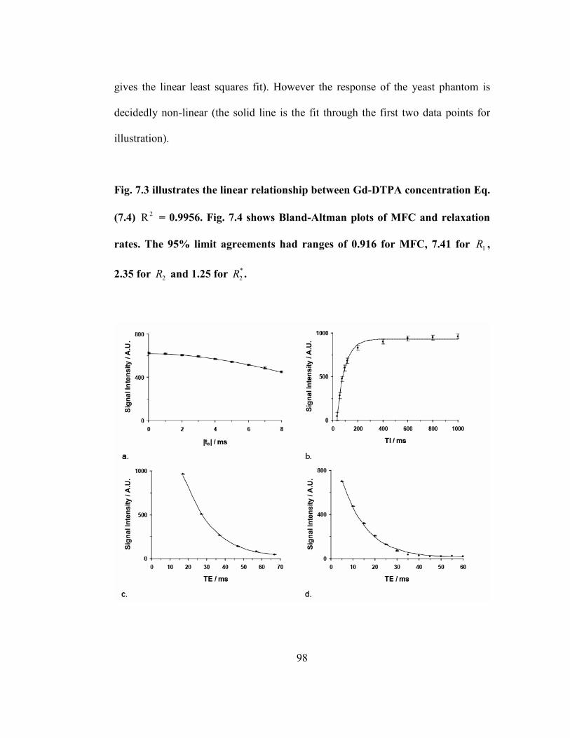
98

gives the linear least squares fit). However the response of the yeast phantom is

decidedly non-linear (the solid line is the fit through the first two data points for

illustration).

Fig. 7.3 illustrates the linear relationship between Gd-DTPA concentration Eq.

(7.4) 2R = 0.9956. Fig. 7.4 shows Bland-Altman plots of MFC and relaxation

rates. The 95% limit agreements had ranges of 0.916 for MFC, 7.41 for 1R ,

2.35 for 2R and 1.25 for *

2R .

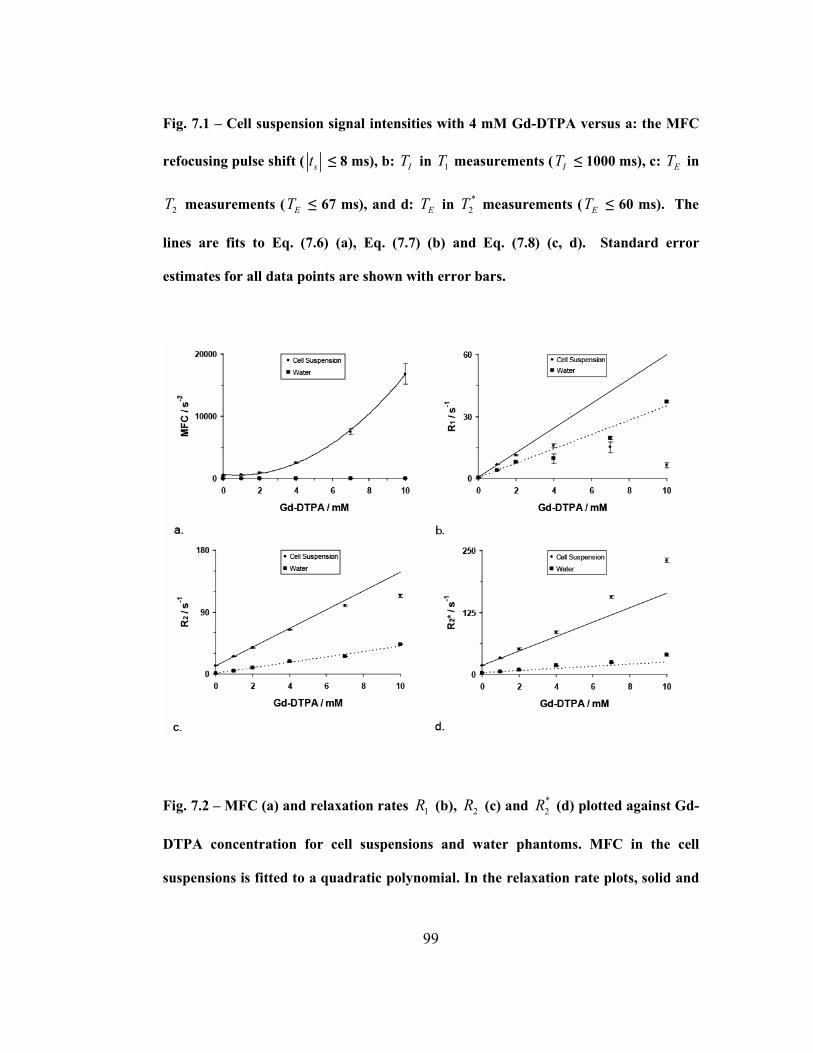
99

Fig. 7.1 – Cell suspension signal intensities with 4 mM Gd-DTPA versus a: the MFC

refocusing pulse shift ( st ≤ 8 ms), b: IT in 1T measurements ( IT ≤ 1000 ms), c: ET in

2T measurements ( ET ≤ 67 ms), and d: ET in *

2T measurements ( ET ≤ 60 ms). The

lines are fits to Eq. (7.6) (a), Eq. (7.7) (b) and Eq. (7.8) (c, d). Standard error

estimates for all data points are shown with error bars.

Fig. 7.2 – MFC (a) and relaxation rates 1R (b), 2R (c) and *

2R (d) plotted against Gd-

DTPA concentration for cell suspensions and water phantoms. MFC in the cell

suspensions is fitted to a quadratic polynomial. In the relaxation rate plots, solid and

100

dashed lines represent a linear extrapolations, based on the [Gd] = 0 and [Gd] = 1

mM data points for the cell suspension and water phantom respectively. Standard

error estimates for all data points are shown with error bars.

Fig. 7.3 – Plot of MFC difference as a function of Gd-DTPA concentration (Eq. (7.4)).

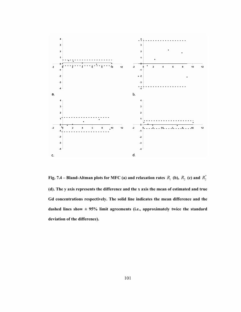
101

Fig. 7.4 – Bland-Altman plots for MFC (a) and relaxation rates 1R (b), 2R (c) and *

2R

(d). The y axis represents the difference and the x axis the mean of estimated and true

Gd concentrations respectively. The solid line indicates the mean difference and the

dashed lines show ± 95% limit agreements (i.e., approximately twice the standard

deviation of the difference).

102

Discussion

This study confirms that MFC measurements depend quadratically on Gd-

DTPA concentration in yeast cell suspensions to a high degree of accuracy. This

dependence is significantly more accurate than the generally assumed linear

dependence of relaxation rates on concentration, supporting the potential of MFC

to more accurately quantify CA concentrations. Comparison of the results from

chapter 4 may not be appropriate since the contrast agent in this study was modeled

to be extravascular and not intravascular.

A study by Tanimoto (2001) demonstrated a linear increase in an agar gel

phantom between superparamagnetic iron oxide (SPIO) contrast agent

concentration and relaxation rates ( 1R , 2R , and *

2R ). However, this linear increase

was not shown in Sephadex bead phantoms except for *

2R rates (52). Fig. 7.2

exhibits substantial deviations from linearity in the cell suspension phantom for

relaxation rates in bottles with [Gd] over 7 mM. Also shown in Fig 7.2. is the

strong quadratic relationship between MFC and Gd-DTPA at all concentrations up

to 10 mM in a cell suspension.

Bland-Altman plots were used to compare each method of measuring [Gd].

These plots are preferable to comparing correlation coefficients a high correlation

does not necessarily imply strong agreement (106). Fig. 7.4 shows that MFC and

*

2R give the best agreement between estimated and true [Gd], with 1R , 2R at least

an order of magnitude worse. *

2R measurements are somewhat easier to make than

103

MFC measurements but the images are heavily susceptible to imaging artifacts due

to macroscopic field inhomogeneities and low signal to noise ratios with increasing

[Gd], both of which may be avoided by using MFC imaging (100).

The range of Gd concentrations used in this study is somewhat larger than

would typically be found in tissues at equilibrium (an average of 0.1 mM with a

standard dose) but might be seen during the first pass of a standard or multiple dose

bolus. Moreover, errors in estimates are of similar size throughout the entire range

of concentrations used here (Fig. 7.4).

This study used gadolinium diethylenetriaminepentaacetic (Gd-DTPA), a

low-molecular weight (< 1000 Da) paramagnetic CA that is the most widely used

contrast agent for human studies. However similar results are expected with other

paramagnetic contrast agents and also those based on iron oxide particles. It should

be noted that Gd-DTPA is water-soluble and homogeneous throughout the cell

suspension. In this study, the distribution of Gd-DTPA was modeled after the

extravascular extracellular space, not the intravascular space. Other factors that

contribute to the complexity of estimating [Gd] are compartmentalization of CA,

geometry of the compartments and the water diffusion rates associated with these

compartments (34).

Finally, the effect that the errors in concentration estimates found here have

on the accuracy of measured perfusion parameters is beyond the scope of this paper

and is the subject of ongoing investigation.

104

CHAPTER 8: Conclusions and Future Directions

Conclusions

This thesis has presented:

1.) An analytical function which models the first-pass of a DSC MRI

concentration-time curve that can be separated into bolus and recirculation

components. Most previous studies model the first-pass by a gamma variate which

does not account for recirculation and requires a method for determining the last

point to fit. These limitations cause inaccuracies and imprecise estimates of the area

under the curve and first moment of the bolus in the presence of noise. However,

the SCR model accurately describes the fist pass plus recirculation and does not

require determination of the last point to fit since it fits the entire concentration-

time curve. The SCR model is less affected by noise.

2.) Empirically determined relaxivity functions in tissue. The results in

chapter 4 confirm that using a linear relaxivity function for quantifying tissue

concentration decreases both accuracy and precision in perfusion estimates. In

contrast, the empirically derived nonlinear function yields precise and accurate

estimates over a range of field strengths and echo times.

3.) Empirically determined relaxivity functions in venous blood. In vitro

experiments using bulk blood phantoms provide useful calibration relaxivity curves

for arterial blood. However, similar experiments with venous blood provide

105

anomalous results. Specifically, an initial decrease in relaxivity as contrast agent

concentration increases which is not seen in vivo. Using the fitting procedure

devised for tissue, we were able to provide accurate relaxivity functions for venous

blood that did not show this anomaly (Chapter 5)

4.) An observation of the reduction of perfusion in normal appearing tissue

in brain cancer patients treated with bevacizumab. Typically, normal appearing

tissue contralateral to the tumor is used as a reference tissue when making relative

CBV measurements. The study conducted in chapter 6 provides strong evidence

that perfusion in the normal appearing tissue of patients treated with bevacizumab

is reduced and thus that relative measurements must be treated with caution.

4.) In vitro demonstration of the accuracy of a new imaging technique,

MFC, in estimating contrast agent concentration. The major advantage of MFC

over traditional relaxation rate measurement is that MFC dependence on

concentration does not depend on contrast agent compartmentalization (i.e., intra-

or extra-vascular).

Future Directions

There still remain a number of issues which must be addressed before DSC

MRI is considered the “gold standard” for measuring brain perfusion.

First, although the SCR model appears empirically to match actual

concentration measurements, it has not theoretical justification. It may be possible

to derive theoretically expressions that take into account i) second pass effects, ii)

106

the exchange of contrast between intra- and extra-vascular spaces that occur before

contrast arrives in the brain and iii) the different path lengths of contrast passing

through different vascular pathways.

Second, while we have identified better empirical relaxivity functions for

tissue and venous blood, discrepancies between experimental and theoretical results

indicate that a complete biophysical explanation of relaxivity has yet to be fully

determined. Future work may directly model the competing contributions to

susceptibility contrast (RBC oxygenation, plasma susceptibility, contrast agent

effects, and vascular geometry) to better understand or improve the nonlinear

relaxivity functions and their theoretical justifications. However, the new relaxivity

functions could now be used to recalibrate clinical perfusion thresholds for

different diagnoses and prognoses.

Third, the relaxivity of extravasated blood must be determined to estimate

contrast agent concentration in areas which are affected by damage to the blood-

brain barrier. MFC is a promising method for this purpose since

compartmentalization does not affect its dependence on concentration. Two

different studies must be performed before MFC can be used for DSC MRI. First,

MFC should be measured before and during the recirculation phase of DSC MRI

experiments (the biological half-life of Gd-DTPA is approximately 7 min to

calibrate the tissue specific parameter, 1a , in normal and abnormal tissue. Second, a

dynamic MFC measurement sequence with 1s temporal resolution sequence must

be developed and tested. Results can then be compared against other perfusion

107

techniques. If successful, MFC may be the first perfusion MRI technique able to

quantify contrast agent concentration accurately in both normal tissue and tissue

suffering from a damaged blood-brain barrier.

Fourth, the rationale for finding accurate relaxivity functions for venous

blood is that venous measurements, being acquire from large vessels, might be used

to correct for partial volume effects on AIF estimates. This has yet to be

demonstrated.

Fifth, this thesis mainly focused on the errors in CBV but the errors in CBF

and MTT should also be examined.

Finally, this thesis has concentrated on DSC MRI, however dynamic

contrast-enhanced (DCE) MRI is an alternative analysis that takes into account

vascular permeability. Although DCE MRI usually uses T1-weighted data, similar

analyses may be performed on T2*-weighted data. The implications of using

improved relaxivity functions with DCE MRI analyses have yet to be studied.

At its inception in the late 1980s, the main criticism of DSC MRI was that,

relative to its major rival, arterial spin labeling, it was “non-quantitative”. However,

since then DSC MRI has been continuously. Nonetheless, DSC MRI is, without

question, the most commonly used perfusion MRI technique for cerebral imaging

in the clinic. With improvements in image quality, better techniques for acquiring

the AIF and improved relaxivity and analysis methods such as those presented in

this thesis, DSC MRI may be on the verge of acceptance as a fully quantitative

method.

108

APPENDIX A

The following is a mathematical proof of Eq. (1.3), V FM= , when using an

instantaneous injection (note: a constant infusion – indicator being introduced

continuously at a constant rate – will not be considered) (11,32,107). Let q be the

quantity of indicator injected at the beginning of a system and ( )c t is the

concentration of indicator at the end of the system. During the time interval t to

t dt+ the amount of indicator that has left the system is the volume – which can be

expressed as Fdt multiplied by ( )c t . Since the total amount of indicator entering

the system must also equal the amount leaving the system

( )0

q c t Fdt∞

= ∫ (A.1)

and F can be calculated by rearranging Eq. (A.1)

( )0

qF

c t dt∞=

∫. (A.2)

The rate at which indicator leaves the system can be expressed as the product of F

and ( )c t and can be modeled as a distribution function, ( )h t , which describes the

distribution of transit times of the indicator in the system normalized to the amount

of indicator

109

( ) ( ) ( )( )

0

Fc t c th t

q c t dt∞= =

∫. (A.3)

Since ( )h t is a distribution function it must follow the following property,

( )0

1.h t∞

=∫ (A.4)

(Introducing ( )h t allows us to quantify indicator in the system as a concentration

and not a finite quantity.) The rate at which the indicator enters and leaves the

system can be expressed as ( )Fh t dt and the volume of indicator is the time is

takes it, t , to leave the system multiplied by the rate,

( )dV tFh t dt= (A.5)

so that the volume of the system, V , is

( ) ( )0 0

.V tFh t dt F th t dt∞ ∞

= =∫ ∫ (A.6)

Because ( )h t is a distribution function of the transit times it should be noticed that

( )0th t dt

∞

∫ is the first moment,

( )0

M th t dt∞

= ∫ (A.7)

and therefore proving the central volume theorem.

In practice, achieving an ideal instantaneous injection where the total

amount of indicator can be introduced into the system at time zero is not practical.

If M is much greater than the injection time then the above proof holds, however

if the injection time is comparable to M then the observed M will be greater than

110

the true M . The following modifications to the proof must be made: First, the

injection can be considered to be a function continuous series of instantaneous

injections, ( )iC t , and each injection is superimposed by a tissue response function,

( )R t , known as the residue function. The resulting distribution of transit times can

be expressed as a convolution.

( ) ( ) ( )0

t

ih t C R t dτ τ τ= −∫ (A.8)

Combining Eqs. (A.4) and (A.8) gives,

( ) ( ) ( )0 0 0

1t

ih t dt C R t d dtτ τ τ∞ ∞

= − =∫ ∫ ∫ (A.9)

and by the additive property of the first moments of convolved function,

( ) ( ) ( )0 0 0

iM th t dt tC t dt tR t dt∞ ∞ ∞

= = +∫ ∫ ∫ (A.10)

Eq. (A.7) is proven for an injection whose injection time is comparable to M .

111

APPENDIX B

The following is a mathematical proof of Eq. (1.10), ( )0

MTT R t dt∞

= ∫ .

The definition of ( )R t is

( ) ( )0

1R t h t dt∞

= − ∫ (B.1)

so that

( ) dRh t

dt= − . (B.2)

Combining Eqs. (A.7) and (B.2),

0

MTTdRt dtdt

∞= −∫ (B.3)

and integrating 0

dRt dtdt

∞−∫ by parts,

( ) [ ]00

MTT R t dt Rt∞ ∞

= −∫ . (B.4)

Since the amount of indicator injected is finite and by definition, again, R

is the amount of indicator remaining in tissue at time, t , lim 0t

Rt→∞

= , Thus proving

Eq. (1.10).

The following is a brief explanation for Eq. (1.12), ( )( )

CBVtH

a

C t dtk

C t dtρ= ∫

∫.

By the principle of conservation of mass and using Eq. (A.1),

112

( ) ( )Ha t

b

k Fq F C t dt C t dt

vρ= =∫ ∫ . (B.5)

Eq. (1.12) is then obtained by rearranging Eq. (B.5)

113

APPENDIX C

Here we sketch the derivation of Eq. (7.3). If the CA is distributed

according to a fixed spatial pattern, then the local magnetic field shift for an

individual water proton depends linearly on the CA concentration so that.

( ) ( ) ( )B t B t C F tδ δ ′= + ⋅ (C.1)

where ( )B tδ ′ is the field shift in the absence of the CA and ( )F t is a function that

depends on the water proton's diffusion path, and where we have assumed a time-

independent concentration. The validity of Eq. (C.1) also requires that ( )B tδ

< 0B and ( )B tδ ′ < 0B , with 0B being the applied field, but these two conditions

are generally well satisfied for clinical scanners. From Eqs. (7.2) and (C.1), one

finds

( ) ( ) ( )

( ) ( ) ( ) ( ) ( ) ( )

2

2 1 1 2

2 2

1 2 1 2 1 2

MFC t t B t B t

C B t F t F t B t C F t F t

γ δ δ

γ δ δ γ

′ ′− = +

′ ′+ + (C.2)

The identifications

( ) ( )2

1 1 2a F t F tγ= (C.3)

( ) ( ) ( ) ( )2

2 1 2 1 2

1

1

2a C B t F t F t B t

aγ δ δ′ ′= +

( ) ( )2 2

3 2 1 1 2a B t B t a aγ δ δ′ ′= −

then lead directly to Eq. (7.3).

114

REFERENCES

1. Stewart GN. Researches on the Circulation Time and on the Influences

which affect it. J Physiol 1897;22(3):159-183.

2. Stolnikow T. Die Aichung des Blutetromes in der Aorta des Hundes. Arch f

Anat u Physiol 1886;19:1-66.

3. Tigerstedt R. Studien ueber die Blutvertheilung im Korper. Skand Arch f

Physiol 1891;3:145.

4. Grehant H, Quinquaud CE. Recherches experimentales sur la mesure du

volume de sang qui traverse les poumons en un temps donne. Compt Rend

Sci Soc Biol 1886;30:159.

5. Fick A. Ueber die Messung des Blutquantums in den Herzventrikeln. Verh

Phys Med Ges Wurzburg 1870;2:16-28.

6. Kety SS, Schmidt CF. The determination of cerebral blood flow in man by

the use of nitrous oxide in low concentrations. Am J Physiol 1945;143:53-

66.

7. Ingvar DH, Cronqvist S, Ekberg R, Risberg J, Hoedt-Rasmussen K. Normal

values of regional cerebral blood flow in man, including flow and weight

estimates of gray and white matter. A preliminary summary. Acta Neurol

Scand Suppl 1965;14:72-78.

115

8. Yamamoto YL, Thompson C, Meyer E, Feindel W. Positron emission

tomography for measurement of regional cerebral blood flow. Adv Neurol

1981;30:41-53.

9. Kuhl DE, Chamberlain RH, Hale J, Gorson RO. A high-contrast

photographic recorder for scintillation counter scanning. Radiology

1956;66(5):730-739.

10. Hounsfield GN. Computerized transverse axial scanning (tomography). 1.

Description of system. Br J Radiol 1973;46(552):1016-1022.

11. Axel L. Cerebral Blood-Flow Determination by Rapid-Sequence

Computed-Tomography - a Theoretical-Analysis. Radiology

1980;137(3):679-686.

12. Miles KA. Brain perfusion: computed tomography applications.

Neuroradiology 2004;46 Suppl 2:s194-200.

13. Williams DS, Detre JA, Leigh JS, Koretsky AP. Magnetic resonance

imaging of perfusion using spin inversion of arterial water. Proc Natl Acad

Sci U S A 1992;89(1):212-216.

14. Petersen ET, Zimine I, Ho YC, Golay X. Non-invasive measurement of

perfusion: a critical review of arterial spin labelling techniques. Br J Radiol

2006;79(944):688-701.

15. Rosen BR, Belliveau JW, Vevea JM, Brady TJ. Perfusion imaging with

NMR contrast agents. Magn Reson Med 1990;14(2):249-265.

116

16. Aronen HJ, Gazit IE, Louis DN, Buchbinder BR, Pardo FS, Weisskoff RM,

Harsh GR, Cosgrove GR, Halpern EF, Hochberg FH, et al. Cerebral blood

volume maps of gliomas: comparison with tumor grade and histologic

findings. Radiology 1994;191(1):41-51.

17. Knopp EA, Cha S, Johnson G, Mazumdar A, Golfinos JG, Zagzag D, Miller

DC, Kelly PJ, Kricheff, II. Glial neoplasms: dynamic contrast-enhanced

T2*-weighted MR imaging. Radiology 1999;211(3):791-798.

18. Johnson G, Wetzel SG, Cha S, Babb J, Tofts PS. Measuring blood volume

and vascular transfer constant from dynamic, T(2)*-weighted contrast-

enhanced MRI. Magn Reson Med 2004;51(5):961-968.

19. Zivadinov R, Bergsland N, Stosic M, Sharma J, Nussenbaum F, Durfee J,

Hani N, Abdelrahman N, Jaisani Z, Minagar A, Hoque R, Munschauer FE,

3rd, Dwyer MG. Use of perfusion- and diffusion-weighted imaging in

differential diagnosis of acute and chronic ischemic stroke and multiple

sclerosis. Neurol Res 2008;30(8):816-826.

20. Li X, Qi J, Xia L, Yu C, Peng W, Hu X, Hu D, Feng D, Hu J, Qiu L, Li H.

Dynamic gadolinium-enhanced MRI in early ischaemia of the proximal

femoral epiphysis--a preliminary study. Clin Radiol 2008;63(10):1149-

1159.

21. Varga AW, Johnson G, Babb JS, Herbert J, Grossman RI, Inglese M. White

matter hemodynamic abnormalities precede sub-cortical gray matter

changes in multiple sclerosis. J Neurol Sci 2009;282(1-2):28-33.

117

22. Cha S, Yang L, Johnson G, Lai A, Chen MH, Tihan T, Wendland M, Dillon

WP. Comparison of microvascular permeability measurements, K(trans),

determined with conventional steady-state T1-weighted and first-pass T2*-

weighted MR imaging methods in gliomas and meningiomas. AJNR Am J

Neuroradiol 2006;27(2):409-417.

23. Law M, Young RJ, Babb JS, Peccerelli N, Chheang S, Gruber ML, Miller

DC, Golfinos JG, Zagzag D, Johnson G. Gliomas: predicting time to

progression or survival with cerebral blood volume measurements at

dynamic susceptibility-weighted contrast-enhanced perfusion MR imaging.

Radiology 2008;247(2):490-498.

24. Chaskis C, Stadnik T, Michotte A, Van Rompaey K, D'Haens J. Prognostic

value of perfusion-weighted imaging in brain glioma: a prospective study.

Acta Neurochir (Wien) 2006;148(3):277-285; discussion 285.

25. Cheng HL. Investigation and optimization of parameter accuracy in

dynamic contrast-enhanced MRI. J Magn Reson Imaging 2008;28(3):736-

743.

26. Lev MH, Ozsunar Y, Henson JW, Rasheed AA, Barest GD, Harsh GRt,

Fitzek MM, Chiocca EA, Rabinov JD, Csavoy AN, Rosen BR, Hochberg

FH, Schaefer PW, Gonzalez RG. Glial tumor grading and outcome

prediction using dynamic spin-echo MR susceptibility mapping compared

with conventional contrast-enhanced MR: confounding effect of elevated

rCBV of oligodendrogliomas [corrected]. AJNR Am J Neuroradiol

2004;25(2):214-221.

118

27. Law M, Yang S, Wang H, Babb JS, Johnson G, Cha S, Knopp EA, Zagzag

D. Glioma grading: sensitivity, specificity, and predictive values of

perfusion MR imaging and proton MR spectroscopic imaging compared

with conventional MR imaging. AJNR Am J Neuroradiol

2003;24(10):1989-1998.

28. Ludemann L, Grieger W, Wurm R, Budzisch M, Hamm B, Zimmer C.

Comparison of dynamic contrast-enhanced MRI with WHO tumor grading

for gliomas. Eur Radiol 2001;11(7):1231-1241.

29. Emblem KE, Nedregaard B, Nome T, Due-Tonnessen P, Hald JK, Scheie

D, Borota OC, Cvancarova M, Bjornerud A. Glioma grading by using

histogram analysis of blood volume heterogeneity from MR-derived

cerebral blood volume maps. Radiology 2008;247(3):808-817.

30. Hakyemez B, Erdogan C, Ercan I, Ergin N, Uysal S, Atahan S. High-grade

and low-grade gliomas: differentiation by using perfusion MR imaging.

Clin Radiol 2005;60(4):493-502.

31. Stewart GN. The pulmonary circulation time, the quantity of blood in the

lungs and the output of the heart. American Journal of Physiology

1921;58(1):20-44.

32. Meier P, Zierler KL. On the Theory of the Indicator-Dilution Method for

Measurement of Blood Flow and Volume. Journal of Applied Physiology

1954;6(12):731-744.

119

33. Yablonskiy DA, Haacke EM. Theory of NMR signal behavior in

magnetically inhomogeneous tissues: the static dephasing regime. Magn

Reson Med 1994;32(6):749-763.

34. Kennan RP, Zhong J, Gore JC. Intravascular susceptibility contrast

mechanisms in tissues. Magn Reson Med 1994;31(1):9-21.

35. Kiselev VG. On the theoretical basis of perfusion measurements by

dynamic susceptibility contrast MRI. Magn Reson Med 2001;46(6):1113-

1122.

36. Rempp KA, Brix G, Wenz F, Becker CR, Guckel F, Lorenz WJ.

Quantification of regional cerebral blood flow and volume with dynamic

susceptibility contrast-enhanced MR imaging. Radiology 1994;193(3):637-

641.

37. Mouridsen K, Christensen S, Gyldensted L, Ostergaard L. Automatic

selection of arterial input function using cluster analysis. Magn Reson Med

2006;55(3):524-531.

38. Bleeker EJ, van Osch MJ, Connelly A, van Buchem MA, Webb AG,

Calamante F. New criterion to aid manual and automatic selection of the

arterial input function in dynamic susceptibility contrast MRI. Magn Reson

Med 2011;65(2):448-456.

39. Calamante F, Gadian DG, Connelly A. Delay and dispersion effects in

dynamic susceptibility contrast MRI: simulations using singular value

decomposition. Magn Reson Med 2000;44(3):466-473.

120

40. Ostergaard L, Weisskoff RM, Chesler DA, Gyldensted C, Rosen BR. High

resolution measurement of cerebral blood flow using intravascular tracer

bolus passages. Part I: Mathematical approach and statistical analysis. Magn

Reson Med 1996;36(5):715-725.

41. Gobbel GT, Fike JR. A deconvolution method for evaluating indicator-

dilution curves. Phys Med Biol 1994;39(11):1833-1854.

42. Wu O, Ostergaard L, Weisskoff RM, Benner T, Rosen BR, Sorensen AG.

Tracer arrival timing-insensitive technique for estimating flow in MR

perfusion-weighted imaging using singular value decomposition with a

block-circulant deconvolution matrix. Magn Reson Med 2003;50(1):164-

174.

43. Andersen IK, Szymkowiak A, Rasmussen CE, Hanson LG, Marstrand JR,

Larsson HB, Hansen LK. Perfusion quantification using Gaussian process

deconvolution. Magn Reson Med 2002;48(2):351-361.

44. Calamante F, Gadian DG, Connelly A. Quantification of bolus-tracking

MRI: Improved characterization of the tissue residue function using

Tikhonov regularization. Magn Reson Med 2003;50(6):1237-1247.

45. Ostergaard L, Sorensen AG, Kwong KK, Weisskoff RM, Gyldensted C,

Rosen BR. High resolution measurement of cerebral blood flow using

intravascular tracer bolus passages. Part II: Experimental comparison and

preliminary results. Magn Reson Med 1996;36(5):726-736.

121

46. Calamante F, Yim PJ, Cebral JR. Estimation of bolus dispersion effects in

perfusion MRI using image-based computational fluid dynamics.

Neuroimage 2003;19(2 Pt 1):341-353.

47. Willats L, Connelly A, Calamante F. Improved deconvolution of perfusion

MRI data in the presence of bolus delay and dispersion. Magn Reson Med

2006;56(1):146-156.

48. Vonken EP, van Osch MJ, Bakker CJ, Viergever MA. Simultaneous

quantitative cerebral perfusion and Gd-DTPA extravasation measurement

with dual-echo dynamic susceptibility contrast MRI. Magn Reson Med

2000;43(6):820-827.

49. Quarles CC, Ward BD, Schmainda KM. Improving the reliability of

obtaining tumor hemodynamic parameters in the presence of contrast agent

extravasation. Magn Reson Med 2005;53(6):1307-1316.

50. Stanisz GJ, Henkelman RM. Gd-DTPA relaxivity depends on

macromolecular content. Magn Reson Med 2000;44(5):665-667.

51. Landis CS, Li X, Telang FW, Coderre JA, Micca PL, Rooney WD, Latour

LL, Vetek G, Palyka I, Springer CS, Jr. Determination of the MRI contrast

agent concentration time course in vivo following bolus injection: effect of

equilibrium transcytolemmal water exchange. Magn Reson Med

2000;44(4):563-574.

52. Tanimoto A, Oshio K, Suematsu M, Pouliquen D, Stark DD. Relaxation

effects of clustered particles. J Magn Reson Imaging 2001;14(1):72-77.

122

53. Akbudak E, Kotys MS, Memisevic D, Conturo TE. Quadraticity and

hematocrit dependence of ∆R2* AIF signals at 3T: a blood phantom study

under physiological conditions. Syllabus of the ISMRM workshop on

Quantitative Cerebral Perfusion Imaging Using MRI: A Technical

Perspective. Venice; 2004. p 10-11.

54. van Osch MJ, van der Grond J, Bakker CJ. Partial volume effects on arterial

input functions: shape and amplitude distortions and their correction. J

Magn Reson Imaging 2005;22(6):704-709.

55. Zhao JM, Clingman CS, Narvainen MJ, Kauppinen RA, van Zijl PC.

Oxygenation and hematocrit dependence of transverse relaxation rates of

blood at 3T. Magn Reson Med 2007;58(3):592-597.

56. Blockley NP, Jiang L, Gardener AG, Ludman CN, Francis ST, Gowland

PA. Field strength dependence of R1 and R2* relaxivities of human whole

blood to ProHance, Vasovist, and deoxyhemoglobin. Magn Reson Med

2008;60(6):1313-1320.

57. Patil V, Johnson G, Jensen JH. Robust quantification of contrast agent (CA)

concentration with magnetic field correlation (MFC) imaging. Magn Reson

Med 2009;62(4):1002-1006.

58. Patil V, Johnson G. DeltaR2 (*) gadolinium-diethylenetriaminepentacetic

acid relaxivity in venous blood. Magn Reson Med 2013;69(4):1104-1108.

59. Patil V, Jensen JH, Johnson G. Intravascular contrast agent T(2) (*)

relaxivity in brain tissue. NMR Biomed 2013;26(4):392-399.

123

60. Calamante F, Connelly A, van Osch MJ. Nonlinear DeltaR*2 effects in

perfusion quantification using bolus-tracking MRI. Magn Reson Med

2009;61(2):486-492.

61. Sutton GC, Karnell J, Nylin G. Studies on the rapidity of complete blood

circulation in man. Am Heart J 1950;39(5):741-748.

62. Sheppard CW. Basic Principles of the Tracer Method Introduction to

Mathematical Tracer Kinetics. New York: John Wiley & Sons, Inc; 1962.

63. Lassen NA, Perl W. Tracer Kinetic Methods in Medical Physiology. New

York: Raven Press; 1979.

64. Chan AA, Nelson AJ. Simplified gamma-variate fitting of perfusion curves.

Biomedical Imaging: Nano to Macro, 2004 IEEE International Symposium

on. Volume 2; 2004. p 1067- 1070.

65. Thompson HK, Jr., Starmer CF, Whalen RE, McIntosh HD. Indicator

Transit Time Considered as a Gamma Variate. Circ Res 1964;14:502-515.

66. Perkio J, Aronen HJ, Kangasmaki A, Liu Y, Karonen J, Savolainen S,

Ostergaard L. Evaluation of four postprocessing methods for determination

of cerebral blood volume and mean transit time by dynamic susceptibility

contrast imaging. Magn Reson Med 2002;47(5):973-981.

67. Madsen MT. A Simplified Formulation of the Gamma Variate Function.

Physics in Medicine and Biology 1992;37(7):1597-1600.

124

68. Lin W, Celik A, Derdeyn C, An H, Lee Y, Videen T, Ostergaard L, Powers

WJ. Quantitative measurements of cerebral blood flow in patients with

unilateral carotid artery occlusion: a PET and MR study. J Magn Reson

Imaging 2001;14(6):659-667.

69. Boxerman JL, Hamberg LM, Rosen BR, Weisskoff RM. MR contrast due to

intravascular magnetic susceptibility perturbations. Magn Reson Med

1995;34(4):555-566.

70. Brooks RA, Vymazal J, Bulte JW, Baumgarner CD, Tran V. Comparison of

T2 relaxation in blood, brain, and ferritin. J Magn Reson Imaging

1995;5(4):446-450.

71. van Osch MJ, Vonken EJ, Viergever MA, van der Grond J, Bakker CJ.

Measuring the arterial input function with gradient echo sequences. Magn

Reson Med 2003;49(6):1067-1076.

72. Bjornerud A, Johansson LO, Briley-Saebo K, Ahlstrom HK. Assessment of

T1 and T2* effects in vivo and ex vivo using iron oxide nanoparticles in

steady state--dependence on blood volume and water exchange. Magn

Reson Med 2002;47(3):461-471.

73. Kjolby BF, Ostergaard L, Kiselev VG. Theoretical model of intravascular

paramagnetic tracers effect on tissue relaxation. Magn Reson Med

2006;56(1):187-197.

125

74. Kiselev VG, Posse S. Analytical model of susceptibility-induced MR signal

dephasing: effect of diffusion in a microvascular network. Magn Reson

Med 1999;41(3):499-509.

75. Semmineh NB, Xu J, Quarles CC. Characterizing the susceptibility

calibration factor in heterogeneous vascular networks. Proceedings of

ISMRM 20th Annual Meeting. Melbourne; 2012.

76. Leenders KL, Beaney RP, Brooks DJ, Lammertsma AA, Heather JD,

McKenzie CG. Dexamethasone treatment of brain tumor patients: effects on

regional cerebral blood flow, blood volume, and oxygen utilization.

Neurology 1985;35(11):1610-1616.

77. Purves WK, David Sadava, Gordon H. Orians, H. Craig Heller. Life: The

Science of Biology. Sunderland, Mass; 2004. 954 p.

78. Lammertsma AA, Brooks DJ, Beaney RP, Turton DR, Kensett MJ, Heather

JD, Marshall J, Jones T. In vivo measurement of regional cerebral

haematocrit using positron emission tomography. J Cereb Blood Flow

Metab 1984;4(3):317-322.

79. Patil V, Johnson G. An Improved Model for Describing the Contrast Bolus

in Perfusion MRI. . Med Phys 2011;38(12):6380-6383.

80. Weisskoff RM, Kiihne S. MRI susceptometry: image-based measurement

of absolute susceptibility of MR contrast agents and human blood. Magn

Reson Med 1992;24(2):375-383.

126

81. Jensen JH, Chandra R. NMR relaxation in tissues with weak magnetic

inhomogeneities. Magn Reson Med 2000;44(1):144-156.

82. An H, Lin W. Quantitative measurements of cerebral blood oxygen

saturation using magnetic resonance imaging. J Cereb Blood Flow Metab

2000;20(8):1225-1236.

83. Kiselev VG, Posse S. Analytical theory of susceptibility induced NMR

signal dephasing in a cerebrovascular network. Phys Rev Lett

1998;81(25):5696-5699.

84. Knutsson L, Borjesson S, Larsson EM, Risberg J, Gustafson L, Passant U,

Stahlberg F, Wirestam R. Absolute quantification of cerebral blood flow in

normal volunteers: correlation between Xe-133 SPECT and dynamic

susceptibility contrast MRI. J Magn Reson Imaging 2007;26(4):913-920.

85. Zaharchuk G, Bammer R, Straka M, Newbould RD, Rosenberg J, Olivot

JM, Mlynash M, Lansberg MG, Schwartz NE, Marks MM, Albers GW,

Moseley ME. Improving dynamic susceptibility contrast MRI measurement

of quantitative cerebral blood flow using corrections for partial volume and

nonlinear contrast relaxivity: A xenon computed tomographic comparative

study. J Magn Reson Imaging 2009;30(4):743-752.

86. Bjornerud A, Emblem KE. A fully automated method for quantitative

cerebral hemodynamic analysis using DSC-MRI. J Cereb Blood Flow

Metab 2010;30(5):1066-1078.

127

87. Patil V, Jensen JH, Johnson G. Direct Measurement of Arterial Input

Function in White Matter. Proceedings of ISMRM 18th Annual Meeting.

Stockholm; 2010.

88. Bahn MM. A single-step method for estimation of local cerebral blood

volume from susceptibility contrast MRI images. Magn Reson Med

1995;33(3):309-317.

89. Kjolby BF, Mikkelsen IK, Pedersen M, Ostergaard L, Kiselev VG. Analysis

of partial volume effects on arterial input functions using gradient echo: a

simulation study. Magn Reson Med 2009;61(6):1300-1309.

90. Vredenburgh JJ, Desjardins A, Herndon JE, 2nd, Dowell JM, Reardon DA,

Quinn JA, Rich JN, Sathornsumetee S, Gururangan S, Wagner M, Bigner

DD, Friedman AH, Friedman HS. Phase II trial of bevacizumab and

irinotecan in recurrent malignant glioma. Clin Cancer Res 2007;13(4):1253-

1259.

91. Narayana A, Gruber D, Kunnakkat S, Golfinos JG, Parker E, Raza S,

Zagzag D, Eagan P, Gruber ML. A clinical trial of bevacizumab,

temozolomide, and radiation for newly diagnosed glioblastoma. J

Neurosurg 2012;116(2):341-345.

92. Simon M, Grone HJ, Johren O, Kullmer J, Plate KH, Risau W, Fuchs E.

Expression of vascular endothelial growth factor and its receptors in human

renal ontogenesis and in adult kidney. Am J Physiol 1995;268(2 Pt 2):F240-

250.

128

93. Narayana A, Kelly P, Golfinos J, Parker E, Johnson G, Knopp E, Zagzag D,

Fischer I, Raza S, Medabalmi P, Eagan P, Gruber ML. Antiangiogenic

therapy using bevacizumab in recurrent high-grade glioma: impact on local

control and patient survival. J Neurosurg 2009;110(1):173-180.

94. Narayana A, Kunnakkat SD, Medabalmi P, Golfinos J, Parker E, Knopp E,

Zagzag D, Eagan P, Gruber D, Gruber ML. Change in pattern of relapse

after antiangiogenic therapy in high-grade glioma. Int J Radiat Oncol Biol

Phys 2012;82(1):77-82.

95. Norden AD, Young GS, Setayesh K, Muzikansky A, Klufas R, Ross GL,

Ciampa AS, Ebbeling LG, Levy B, Drappatz J, Kesari S, Wen PY.

Bevacizumab for recurrent malignant gliomas: efficacy, toxicity, and

patterns of recurrence. Neurology 2008;70(10):779-787.

96. Iwamoto FM, Abrey LE, Beal K, Gutin PH, Rosenblum MK, Reuter VE,

DeAngelis LM, Lassman AB. Patterns of relapse and prognosis after

bevacizumab failure in recurrent glioblastoma. Neurology

2009;73(15):1200-1206.

97. de Groot M, Douw L, Sizoo EM, Bosma I, Froklage FE, Heimans JJ,

Postma TJ, Klein M, Reijneveld JC. Levetiracetam improves verbal

memory in high-grade glioma patients. Neuro Oncol 2013;15(2):216-223.

98. Fischer I, Cunliffe CH, Bollo RJ, Raza S, Monoky D, Chiriboga L, Parker

EC, Golfinos JG, Kelly PJ, Knopp EA, Gruber ML, Zagzag D, Narayana A.

High-grade glioma before and after treatment with radiation and Avastin:

initial observations. Neuro Oncol 2008;10(5):700-708.

129

99. Paulson ES, Schmainda KM. Comparison of dynamic susceptibility-

weighted contrast-enhanced MR methods: recommendations for measuring

relative cerebral blood volume in brain tumors. Radiology 2008;249(2):601-

613.

100. Jensen JH, Chandra R, Ramani A, Lu H, Johnson G, Lee SP, Kaczynski K,

Helpern JA. Magnetic field correlation imaging. Magn Reson Med

2006;55(6):1350-1361.

101. Jensen JH, Szulc K, Hu C, Ramani A, Lu H, Xuan L, Falangola MF,

Chandra R, Knopp EA, Schenck J, Zimmerman EA, Helpern JA. Magnetic

field correlation as a measure of iron-generated magnetic field

inhomogeneities in the brain. Magn Reson Med 2009;61(2):481-485.

102. Ethofer T, Mader I, Seeger U, Helms G, Erb M, Grodd W, Ludolph A,

Klose U. Comparison of longitudinal metabolite relaxation times in

different regions of the human brain at 1.5 and 3 Tesla. Magn Reson Med

2003;50(6):1296-1301.

103. Mlynarik V, Gruber S, Moser E. Proton T (1) and T (2) relaxation times of

human brain metabolites at 3 Tesla. NMR Biomed 2001;14(5):325-331.

104. Stanisz GJ, Odrobina EE, Pun J, Escaravage M, Graham SJ, Bronskill MJ,

Henkelman RM. T1, T2 relaxation and magnetization transfer in tissue at

3T. Magn Reson Med 2005;54(3):507-512.

105. Wansapura JP, Holland SK, Dunn RS, Ball WS, Jr. NMR relaxation times

in the human brain at 3.0 tesla. J Magn Reson Imaging 1999;9(4):531-538.

130

106. Bland JM, Altman DG. Statistical methods for assessing agreement between

two methods of clinical measurement. Lancet 1986;1(8476):307-310.

107. Zierler KL. Theoretical Basis of Indicator-Dilution Methods for Measuring

Flow and Volume. Circulation Research 1962;10(3):393-&.