Towards a Unified Theory of Cycles

by Ray Tomes

Paper Presented atFoundation for the Study of Cycles

Conference Proceedings February 1990

made available byCycles Research Institute

http://www.cyclesresearchinstitute.org/

Many thanks to Michael Taler who encouraged me and assisted in the preparation for presentation of this paper in 1989.

Note by the Author, June 2005. This paper is being made available through Cycles ResearchInstitute more than 15 years after its original preparation and presentation. Considerabledevelopments have happened since then:

* The Foundation for the Study of Cycles has ceased to exist.

* Cycles Research Institute has started in a small way to try and re-establish cycles research.

* Much work has been done on the Harmonics Theory first presented in this paper. Although thecorrect calculation was derived before publication of this paper, a slightly different calculation waspresented here. It incorrectly results in the dominant cycles always being related by ratios of 2.

* This paper presents ideas on understanding irregular cycles in planetary configurations that arevery little known, specifically average cycles versus specific occurrences.

* The relativistic gravitational effect of the planets on the Sun outlined here has been presented ina later paper. However the discussion of how this idea came about and problems with both theCOM and tidal theories are presented here.

Towards a Unified Theory of Cycles

by Ray Tomes

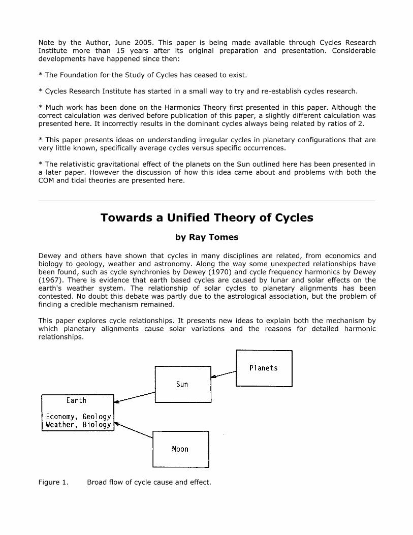
Dewey and others have shown that cycles in many disciplines are related, from economics andbiology to geology, weather and astronomy. Along the way some unexpected relationships havebeen found, such as cycle synchronies by Dewey (1970) and cycle frequency harmonics by Dewey(1967). There is evidence that earth based cycles are caused by lunar and solar effects on theearth's weather system. The relationship of solar cycles to planetary alignments has beencontested. No doubt this debate was partly due to the astrological association, but the problem offinding a credible mechanism remained.

This paper explores cycle relationships. It presents new ideas to explain both the mechanism bywhich planetary alignments cause solar variations and the reasons for detailed harmonicrelationships.

Figure 1. Broad flow of cycle cause and effect.

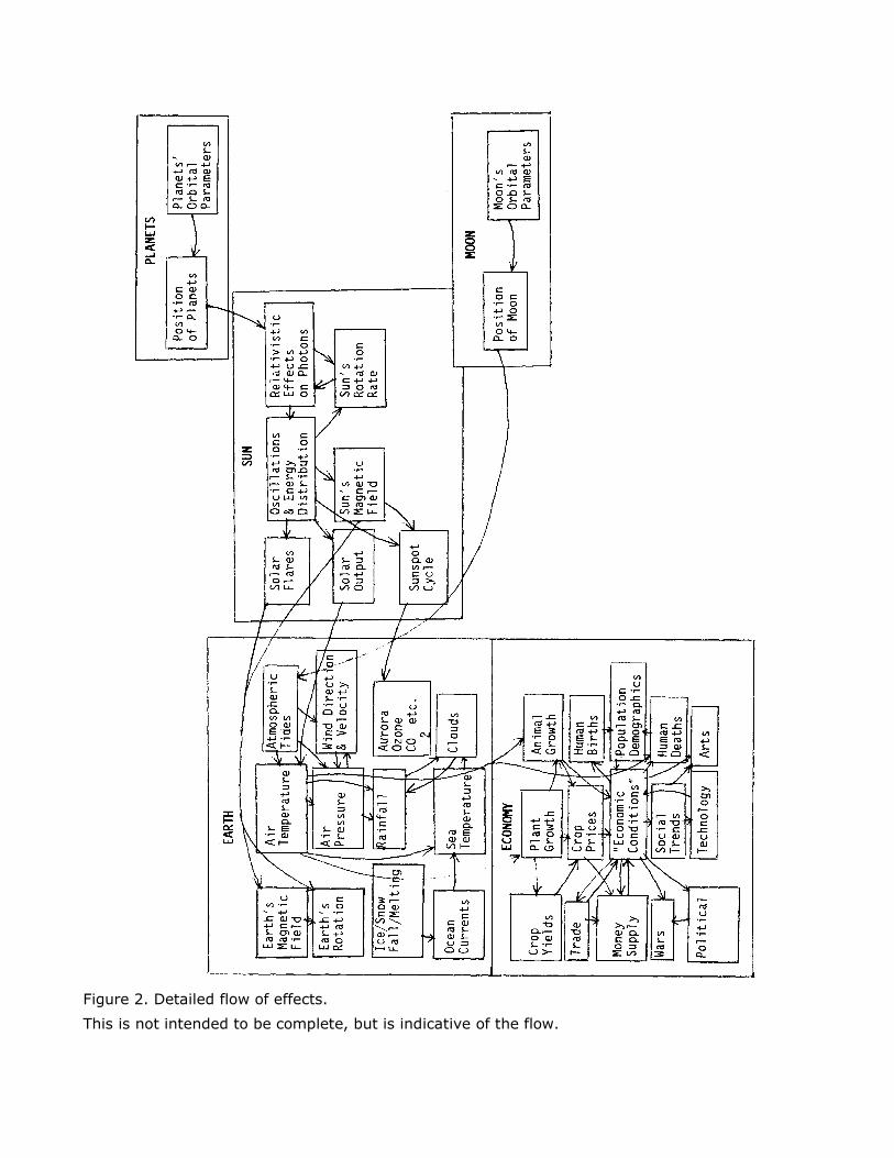
Figure 2. Detailed flow of effects.

This is not intended to be complete, but is indicative of the flow.

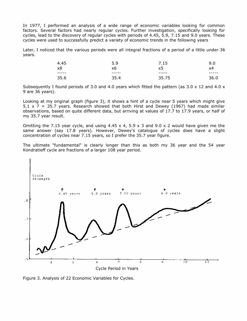
In 1977, I performed an analysis of a wide range of economic variables looking for commonfactors. Several factors had nearly regular cycles. Further investigation, specifically looking forcycles, lead to the discovery of regular cycles with periods of 4.45, 5.9, 7.15 and 9.0 years. Thesecycles were used to successfully predict a variety of economic trends in the following years

Later, I noticed that the various periods were all integral fractions of a period of a little under 36years.

4.45 5.9 7.15 9.0x8 x6 x5 x4----- ----- ----- -----35.6 35.4 35.75 36.0

Subsequently I found periods of 3.0 and 4.0 years which fitted the pattern (as 3.0 x 12 and 4.0 x9 are 36 years).

Looking at my original graph (figure 3), it shows a hint of a cycle near 5 years which might give5.1 x 7 = 35.7 years. Research showed that both Hirst and Dewey (1967) had made similarobservations, based on quite different data, but arriving at values of 17.7 to 17.9 years, or half ofmy 35.7 year result.

Omitting the 7.15 year cycle, and using 4.45 x 4, 5.9 x 3 and 9.0 x 2 would have given me thesame answer (say 17.8 years). However, Dewey's catalogue of cycles does have a slightconcentration of cycles near 7.15 years, so I prefer the 35.7 year figure.

The ultimate "fundamental" is clearly longer than this as both my 36 year and the 54 yearKondratieff cycle are fractions of a larger 108 year period.

Cycle Period in Years

Figure 3. Analysis of 22 Economic Variables for Cycles.

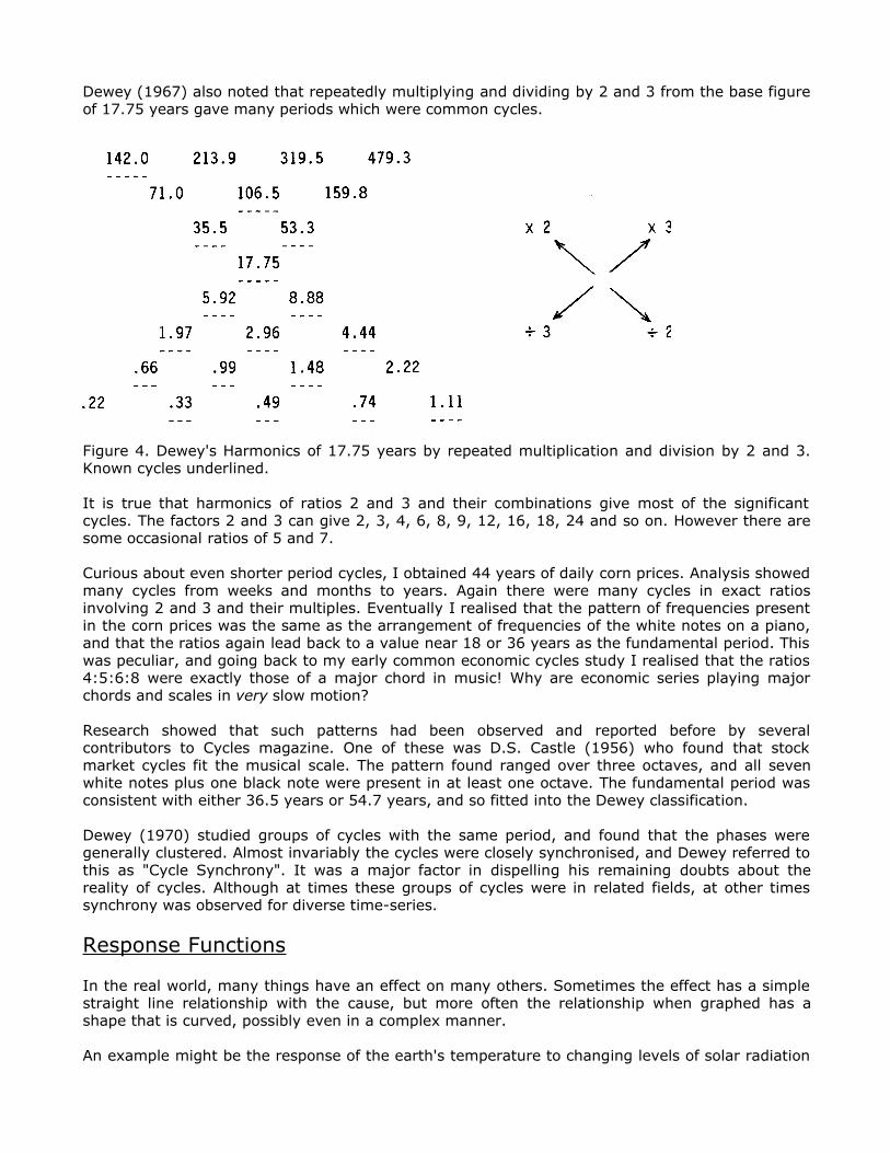
Dewey (1967) also noted that repeatedly multiplying and dividing by 2 and 3 from the base figureof 17.75 years gave many periods which were common cycles.

Figure 4. Dewey's Harmonics of 17.75 years by repeated multiplication and division by 2 and 3.Known cycles underlined.

It is true that harmonics of ratios 2 and 3 and their combinations give most of the significantcycles. The factors 2 and 3 can give 2, 3, 4, 6, 8, 9, 12, 16, 18, 24 and so on. However there aresome occasional ratios of 5 and 7.

Curious about even shorter period cycles, I obtained 44 years of daily corn prices. Analysis showedmany cycles from weeks and months to years. Again there were many cycles in exact ratiosinvolving 2 and 3 and their multiples. Eventually I realised that the pattern of frequencies presentin the corn prices was the same as the arrangement of frequencies of the white notes on a piano,and that the ratios again lead back to a value near 18 or 36 years as the fundamental period. Thiswas peculiar, and going back to my early common economic cycles study I realised that the ratios4:5:6:8 were exactly those of a major chord in music! Why are economic series playing majorchords and scales in very slow motion?

Research showed that such patterns had been observed and reported before by severalcontributors to Cycles magazine. One of these was D.S. Castle (1956) who found that stockmarket cycles fit the musical scale. The pattern found ranged over three octaves, and all sevenwhite notes plus one black note were present in at least one octave. The fundamental period wasconsistent with either 36.5 years or 54.7 years, and so fitted into the Dewey classification.

Dewey (1970) studied groups of cycles with the same period, and found that the phases weregenerally clustered. Almost invariably the cycles were closely synchronised, and Dewey referred tothis as "Cycle Synchrony". It was a major factor in dispelling his remaining doubts about thereality of cycles. Although at times these groups of cycles were in related fields, at other timessynchrony was observed for diverse time-series.

Response Functions

In the real world, many things have an effect on many others. Sometimes the effect has a simplestraight line relationship with the cause, but more often the relationship when graphed has ashape that is curved, possibly even in a complex manner.

An example might be the response of the earth's temperature to changing levels of solar radiation

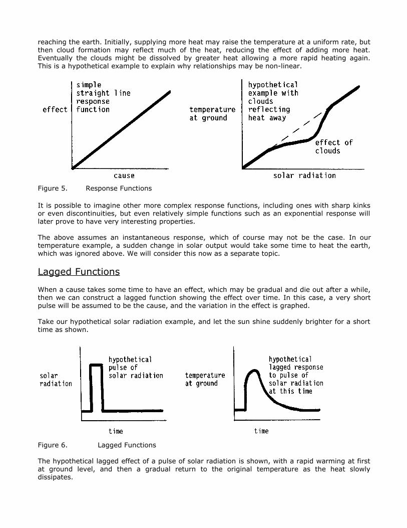
reaching the earth. Initially, supplying more heat may raise the temperature at a uniform rate, butthen cloud formation may reflect much of the heat, reducing the effect of adding more heat.Eventually the clouds might be dissolved by greater heat allowing a more rapid heating again.This is a hypothetical example to explain why relationships may be non-linear.

Figure 5. Response Functions

It is possible to imagine other more complex response functions, including ones with sharp kinksor even discontinuities, but even relatively simple functions such as an exponential response willlater prove to have very interesting properties.

The above assumes an instantaneous response, which of course may not be the case. In ourtemperature example, a sudden change in solar output would take some time to heat the earth,which was ignored above. We will consider this now as a separate topic.

Lagged Functions

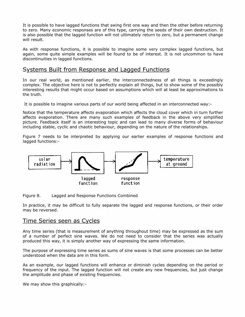
When a cause takes some time to have an effect, which may be gradual and die out after a while,then we can construct a lagged function showing the effect over time. In this case, a very shortpulse will be assumed to be the cause, and the variation in the effect is graphed.

Take our hypothetical solar radiation example, and let the sun shine suddenly brighter for a shorttime as shown.

Figure 6. Lagged Functions

The hypothetical lagged effect of a pulse of solar radiation is shown, with a rapid warming at firstat ground level, and then a gradual return to the original temperature as the heat slowlydissipates.

It is possible to have lagged functions that swing first one way and then the other before returningto zero. Many economic responses are of this type, carrying the seeds of their own destruction. Itis also possible that the lagged function will not ultimately return to zero, but a permanent changewill result.

As with response functions, it is possible to imagine some very complex lagged functions, butagain, some quite simple examples will be found to be of interest. It is not uncommon to havediscontinuities in lagged functions.

Systems Built from Response and Lagged Functions

In our real world, as mentioned earlier, the interconnectedness of all things is exceedinglycomplex. The objective here is not to perfectly explain all things, but to show some of the possiblyinteresting results that might occur based on assumptions which will at least be approximations tothe truth.

It is possible to imagine various parts of our world being affected in an interconnected way:-

Notice that the temperature affects evaporation which affects the cloud cover which in turn furtheraffects evaporation. There are many such examples of feedback in the above very simplifiedpicture. Feedback itself is an interesting topic and can lead to many diverse forms of behaviourincluding stable, cyclic and chaotic behaviour, depending on the nature of the relationships.

Figure 7 needs to be interpreted by applying our earlier examples of response functions andlagged functions:-

Figure 8. Lagged and Response Functions Combined

In practice, it may be difficult to fully separate the lagged and response functions, or their ordermay be reversed.

Time Series seen as Cycles

Any time series (that is measurement of anything throughout time) may be expressed as the sumof a number of perfect sine waves. We do not need to consider that the series was actuallyproduced this way, it is simply another way of expressing the same information.

The purpose of expressing time series as sums of sine waves is that some processes can be betterunderstood when the data are in this form.

As an example, our lagged functions will enhance or diminish cycles depending on the period orfrequency of the input. The lagged function will not create any new frequencies, but just changethe amplitude and phase of existing frequencies.

We may show this graphically:-

Figure 9. Response Function effect of frequency on amplitude

In this example, frequencies in the range A to B are enhanced, while all others are diminished.Very high frequencies are not responded to at all. This might be the frequency response of oursolar radiation - temperature example.

Harmonics are created by non-linear Response Functions

If we feed sine waves into different response functions, the result is quite surprising. The output isalways a time series which is the sum of various sine waves that are all harmonics of the originalwave. By harmonics we mean frequencies that are integer multiples of the original frequency.

This means that in this case the input and output would look like:-

Figure 10. Development of Harmonics by Response Function

Notice that the first harmonic output is in phase (or 180 degrees out of phase) with the input in allcases. This results in cycle synchronies even after multiple steps in a cause and effect chain andhelps explain Dewey's observations.

Some other examples of response functions and their makeup from harmonics are shown below.In no case can any frequency be created which is not an exact multiple of the input frequency.

Note - not true for multiple input frequencies when sums and differences of frequencies mayresult. Figure 11. Examples of Harmonics for various Response Functions

All Harmonics are not equal in complex systems

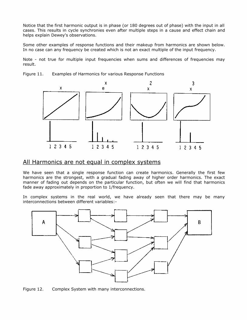
We have seen that a single response function can create harmonics. Generally the first fewharmonics are the strongest, with a gradual fading away of higher order harmonics. The exactmanner of fading out depends on the particular function, but often we will find that harmonicsfade away approximately in proportion to 1/frequency.

In complex systems in the real world, we have already seen that there may be manyinterconnections between different variables:-

Figure 12. Complex System with many interconnections.

We shall consider a collection of response functions, with many paths from A to B, but without anyfeedback. In practice, feedback nearly always exists, but it can complicate things by creating newcycles, and for the moment we only wish to investigate the creation of harmonics.

Some harmonics can be created in more ways than others. For example, the fifth harmonic canonly be created in one way, as 5 is a prime number. The sixth harmonic however can be created inthree ways, either directly as 6 or indirectly as 2 x 3 or 3 x 2. Some harmonics can be created invery many ways for example 24 has twenty different ways of being created and 576 has 1,376ways!

In B we would therefore expect the 6th, 24th and 576th harmonics of a frequency in A to be muchstronger than the 5th, 23rd and 577th which each have only one way of being created.

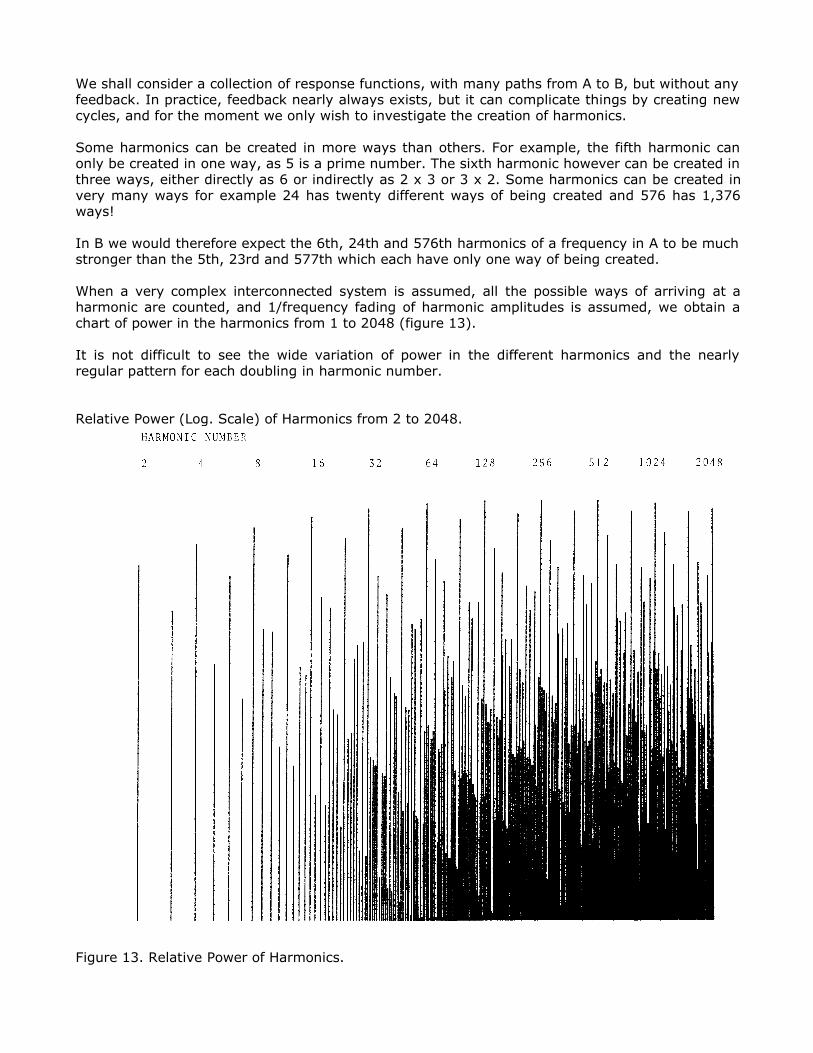
When a very complex interconnected system is assumed, all the possible ways of arriving at aharmonic are counted, and 1/frequency fading of harmonic amplitudes is assumed, we obtain achart of power in the harmonics from 1 to 2048 (figure 13).

It is not difficult to see the wide variation of power in the different harmonics and the nearlyregular pattern for each doubling in harmonic number.

Relative Power (Log. Scale) of Harmonics from 2 to 2048.

Figure 13. Relative Power of Harmonics.

Let there be Music

If we look at one part of the structure, for example the "octave" from 48 through to 96, we findthat the harmonics with most power are:-

Table 1. Most Powerful Harmonics related to musical scale.

Harmonic 48 54 60 64 72 80 84 90 96

Note C D E F G A Bb B C

Amazingly, the nine most powerful harmonics turn out to have frequencies inthe same ratios as the eight white notes in one octave on the piano plus one black note. Also, theone black note Bb is required to make the chord of C7 along with C-E-G-C. The strongest notesare in the two chords C-F-A-C (F major) and C-E-G-C (C major).

The assignment of C to harmonic 48 is quite arbitrary, but this choice was made because themajor scale of C is all white notes. The choice of the "octave" from harmonic 48 to 96 was alsosomewhat arbitrary. Different octaves have different power distributions of the individual "notes".As we go up the harmonics scale, the relative power of the notes in each octave changesgradually, but at a diminishing rate.

Well that is rather interesting, we started out trying to find out which harmonics are expected tobe generated in time series after going through complex systems of response functions, andended up explaining how the notes used in music are exactly as they are, and what the mainchords should be!

Background to Planets' Influence on the Sun

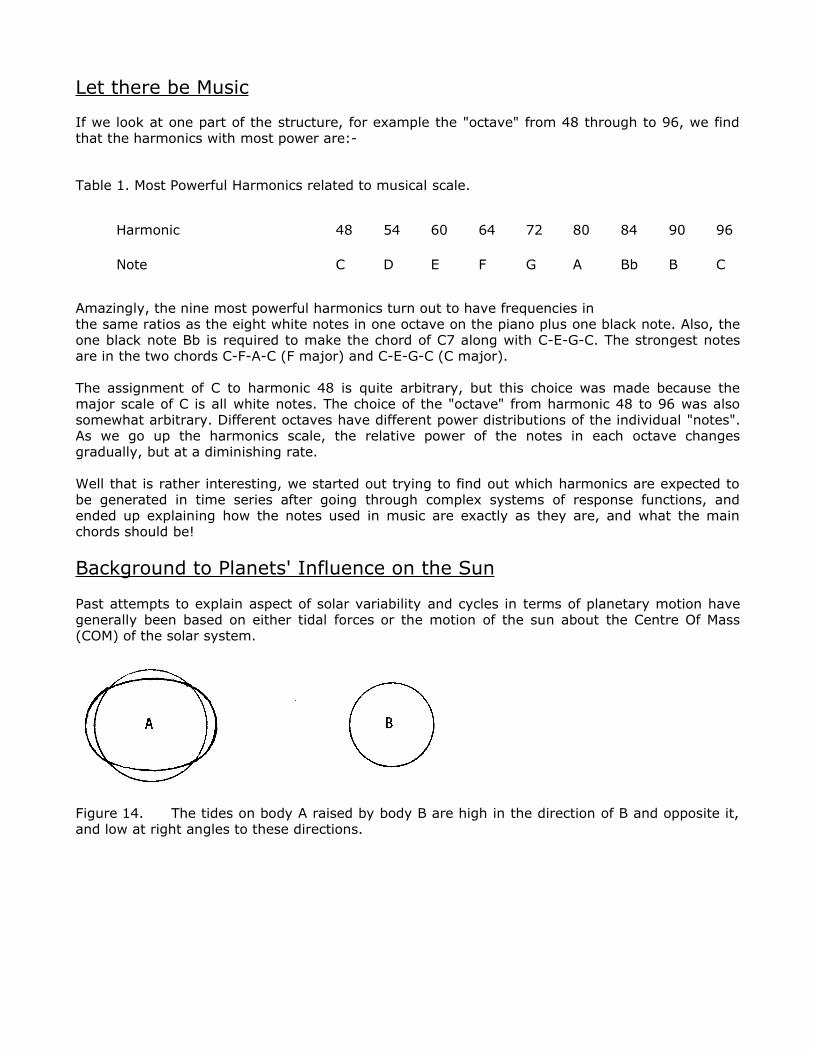
Past attempts to explain aspect of solar variability and cycles in terms of planetary motion havegenerally been based on either tidal forces or the motion of the sun about the Centre Of Mass(COM) of the solar system.

Figure 14. The tides on body A raised by body B are high in the direction of B and opposite it,and low at right angles to these directions.

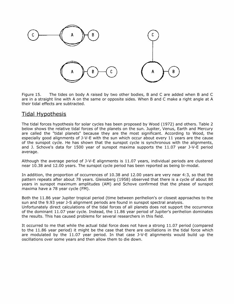
Figure 15. The tides on body A raised by two other bodies, B and C are added when B and Care in a straight line with A on the same or opposite sides. When B and C make a right angle at Atheir tidal effects are subtracted.

Tidal Hypothesis

The tidal forces hypothesis for solar cycles has been proposed by Wood (1972) and others. Table 2below shows the relative tidal forces of the planets on the sun. Jupiter, Venus, Earth and Mercuryare called the "tidal planets" because they are the most significant. According to Wood, theespecially good alignments of J-V-E with the sun which occur about every 11 years are the causeof the sunspot cycle. He has shown that the sunspot cycle is synchronous with the alignments,and J. Schove's data for 1500 year of sunspot maxima supports the 11.07 year J-V-E periodaverage.

Although the average period of J-V-E alignments is 11.07 years, individual periods are clusterednear 10.38 and 12.00 years. The sunspot cycle period has been reported as being bi-modal.

In addition, the proportion of occurrences of 10.38 and 12.00 years are very near 4:3, so that thepattern repeats after about 78 years. Gleissberg (1958) observed that there is a cycle of about 80years in sunspot maximum amplitudes (AM) and Schove confirmed that the phase of sunspotmaxima have a 78 year cycle (FM).

Both the 11.86 year Jupiter tropical period (time between perihelion's or closest approaches to thesun and the 9.93 year J-S alignment periods are found in sunspot spectral analysis.Unfortunately direct calculations of the tidal forces of all planets does not support the occurrenceof the dominant 11.07 year cycle. Instead, the 11.86 year period of Jupiter's perihelion dominatesthe results. This has caused problems for several researchers in this field.

It occurred to me that while the actual tidal force does not have a strong 11.07 period (comparedto the 11.86 year period) it might be the case that there are oscillations in the tidal force whichare modulated by the 11.07 year period. In that case J-V-E alignments would build up theoscillations over some years and then allow them to die down.

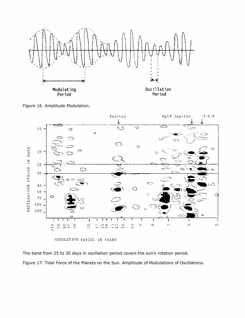
Figure 16. Amplitude Modulation.

The band from 25 to 30 days in oscillation period covers the sun's rotation period.

Figure 17. Tidal Force of the Planets on the Sun. Amplitude of Modulations of Oscillations.

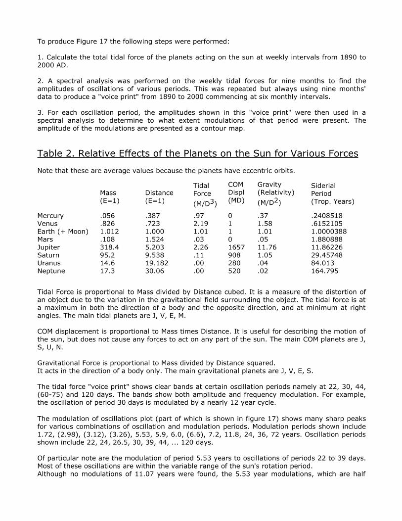
To produce Figure 17 the following steps were performed:

1. Calculate the total tidal force of the planets acting on the sun at weekly intervals from 1890 to2000 AD.

2. A spectral analysis was performed on the weekly tidal forces for nine months to find theamplitudes of oscillations of various periods. This was repeated but always using nine months'data to produce a "voice print" from 1890 to 2000 commencing at six monthly intervals.

3. For each oscillation period, the amplitudes shown in this "voice print" were then used in aspectral analysis to determine to what extent modulations of that period were present. Theamplitude of the modulations are presented as a contour map.

Table 2. Relative Effects of the Planets on the Sun for Various Forces

Note that these are average values because the planets have eccentric orbits.

Mass(E=1)

Distance(E=1)

TidalForce

(M/D3)

COMDispl(MD)

Gravity(Relativity)

(M/D2)

SiderialPeriod(Trop. Years)

Mercury .056 .387 .97 0 .37 .2408518Venus .826 .723 2.19 1 1.58 .6152105Earth (+ Moon) 1.012 1.000 1.01 1 1.01 1.0000388Mars .108 1.524 .03 0 .05 1.880888Jupiter 318.4 5.203 2.26 1657 11.76 11.86226Saturn 95.2 9.538 .11 908 1.05 29.45748Uranus 14.6 19.182 .00 280 .04 84.013Neptune 17.3 30.06 .00 520 .02 164.795

Tidal Force is proportional to Mass divided by Distance cubed. It is a measure of the distortion ofan object due to the variation in the gravitational field surrounding the object. The tidal force is ata maximum in both the direction of a body and the opposite direction, and at minimum at rightangles. The main tidal planets are J, V, E, M.

COM displacement is proportional to Mass times Distance. It is useful for describing the motion ofthe sun, but does not cause any forces to act on any part of the sun. The main COM planets are J,S, U, N.

Gravitational Force is proportional to Mass divided by Distance squared.It acts in the direction of a body only. The main gravitational planets are J, V, E, S.

The tidal force "voice print" shows clear bands at certain oscillation periods namely at 22, 30, 44,(60-75) and 120 days. The bands show both amplitude and frequency modulation. For example,the oscillation of period 30 days is modulated by a nearly 12 year cycle.

The modulation of oscillations plot (part of which is shown in figure 17) shows many sharp peaksfor various combinations of oscillation and modulation periods. Modulation periods shown include1.72, (2.98), (3.12), (3.26), 5.53, 5.9, 6.0, (6.6), 7.2, 11.8, 24, 36, 72 years. Oscillation periodsshown include 22, 24, 26.5, 30, 39, 44, ... 120 days.

Of particular note are the modulation of period 5.53 years to oscillations of periods 22 to 39 days.Most of these oscillations are within the variable range of the sun's rotation period.Although no modulations of 11.07 years were found, the 5.53 year modulations, which are half

the 11.07 period gave a pointer to the fact that the correct force was not tidal, but directgravitational as tidal forces have double the frequencies.

COM Hypothesis

The motion of the sun about the COM of the solar system does not give any reasonableexplanation for the 11 year sunspot cycle. It does have some success at explaining the longerterm modulations, of 80-90 years and 170-180 years. Jupiter, Saturn, Uranus and Neptune arethe planets which affect the sun's motion about the COM the most. The dominant period is theJupiter-Saturn Synodic period of 19.86 years. The 9.93 year component in the sunspot spectrumcould be related to this (being half of 19.86 years).

If the COM hypothesis were true, then the most distant stars in the universe would have anenormous effect on the sun due to their distance. This seems absurd.

A Planetary Solar Influence Mechanism

My research showed that the 11 year solar cycle must be the result of modulations of shorter (ofthe order of the sun's rotation) period oscillations.

The tidal hypothesis predicted cycles with double the required frequency, which leads to theconclusion that the correct force is gravitational not tidal.

I believe that the correct mechanism is a relativistic effect of gravity.

Einstein showed that light travelling past the sun would be bent twice as much as expected byclassical physics. This was shown to be correct by observations of stars during eclipses. Until nowit seems that no-one has applied these equations to the planets' gravitational effect on photonsinside the sun. As well as an effect on photons in the sun, there will be lesser effects on matter inthe solar interior, which because of its high temperature will have slightly relativistic velocities.

The planets accelerate the sun by an amount that causes the sun to move about (relative to theCOM of the solar system) by several times its own radius over a period of years. Thereforephotons contained in the sun have forces acting on them sufficiently different to those acting onthe matter to displace the photons by several solar radii were they free to do so. Photons in thesun are contained for long periods due to frequent deflections by matter.

As the planets' gravity displaces the photons, the sun's rotation carries the photons around.Therefore the planetary force does not accumulate in one direction. Instead, only OSCILLATIONSin the planetary forces that closely match the sun's rotation period are able to build up over time.Such oscillations do exist because of the changing alignments of the planets and the non-linearrelationship of gravity. Harmonics of the planets' orbital and synodic period have frequencieswithin the range of the solar rotation.

The sun rotates at significantly different rates at different latitudes, depths and times. Thiscomplicates the calculations required to model the relativistic effects, which in turn are probablythe cause of the variable rotation.

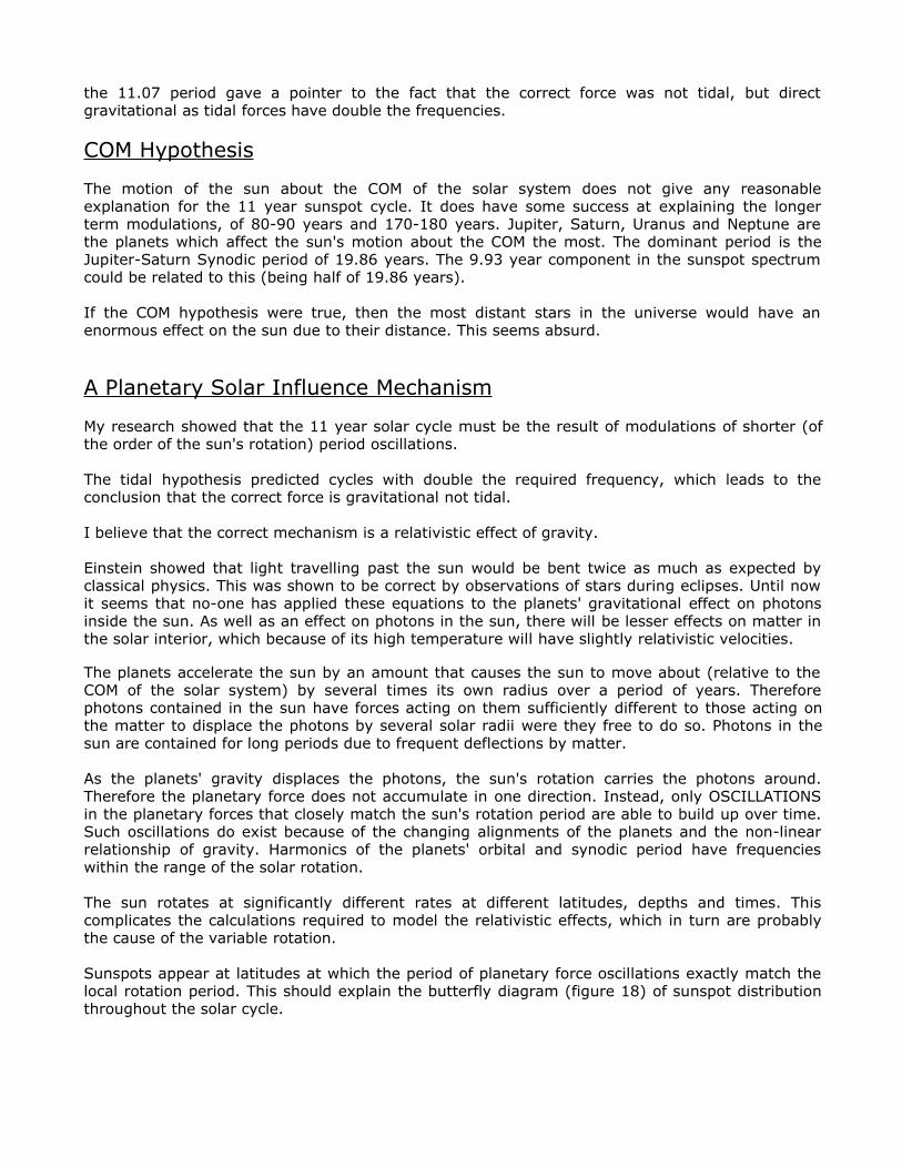
Sunspots appear at latitudes at which the period of planetary force oscillations exactly match thelocal rotation period. This should explain the butterfly diagram (figure 18) of sunspot distributionthroughout the solar cycle.

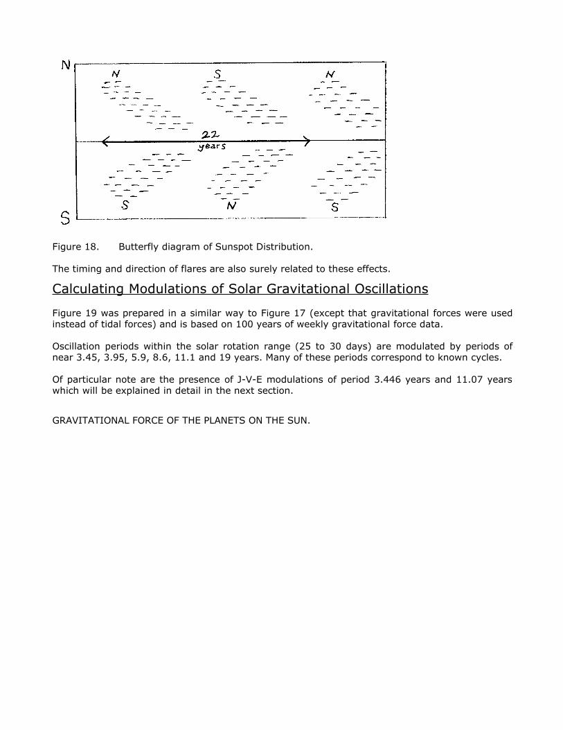
Figure 18. Butterfly diagram of Sunspot Distribution.

The timing and direction of flares are also surely related to these effects.

Calculating Modulations of Solar Gravitational Oscillations

Figure 19 was prepared in a similar way to Figure 17 (except that gravitational forces were usedinstead of tidal forces) and is based on 100 years of weekly gravitational force data.

Oscillation periods within the solar rotation range (25 to 30 days) are modulated by periods ofnear 3.45, 3.95, 5.9, 8.6, 11.1 and 19 years. Many of these periods correspond to known cycles.

Of particular note are the presence of J-V-E modulations of period 3.446 years and 11.07 yearswhich will be explained in detail in the next section.

GRAVITATIONAL FORCE OF THE PLANETS ON THE SUN.

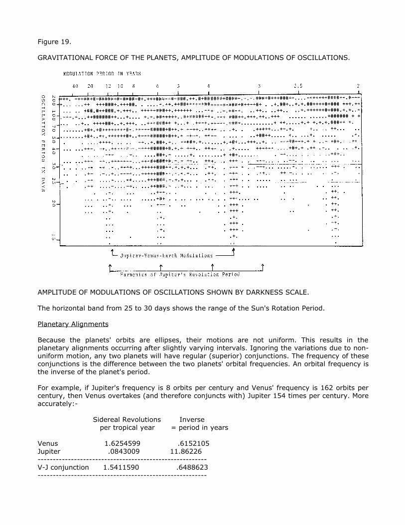
Figure 19.

GRAVITATIONAL FORCE OF THE PLANETS, AMPLITUDE OF MODULATIONS OF OSCILLATIONS.

AMPLITUDE OF MODULATIONS OF OSCILLATIONS SHOWN BY DARKNESS SCALE.

The horizontal band from 25 to 30 days shows the range of the Sun's Rotation Period.

Planetary Alignments

Because the planets' orbits are ellipses, their motions are not uniform. This results in theplanetary alignments occurring after slightly varying intervals. Ignoring the variations due to non-uniform motion, any two planets will have regular (superior) conjunctions. The frequency of theseconjunctions is the difference between the two planets' orbital frequencies. An orbital frequency isthe inverse of the planet's period.

For example, if Jupiter's frequency is 8 orbits per century and Venus' frequency is 162 orbits percentury, then Venus overtakes (and therefore conjuncts with) Jupiter 154 times per century. Moreaccurately:-

Sidereal Revolutions Inverse per tropical year = period in years

Venus 1.6254599 .6152105Jupiter .0843009 11.86226--------------------------------------------------------V-J conjunction 1.5411590 .6488623--------------------------------------------------------

For two planet alignments, this period can be used to accurately calculate conjunctions forwardsor backwards for thousands of years.

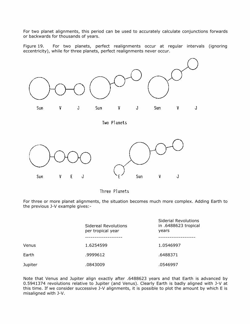
Figure 19. For two planets, perfect realignments occur at regular intervals (ignoringeccentricity), while for three planets, perfect realignments never occur.

For three or more planet alignments, the situation becomes much more complex. Adding Earth tothe previous J-V example gives:-

Sidereal Revolutionsper tropical year

Siderial Revolutionsin .6488623 tropicalyears

-------------------- --------------------

Venus 1.6254599 1.0546997

Earth .9999612 .6488371

Jupiter .0843009 .0546997

Note that Venus and Jupiter align exactly after .6488623 years and that Earth is advanced by0.5941374 revolutions relative to Jupiter (and Venus). Clearly Earth is badly aligned with J-V atthis time. If we consider successive J-V alignments, it is possible to plot the amount by which E ismisaligned with J-V.

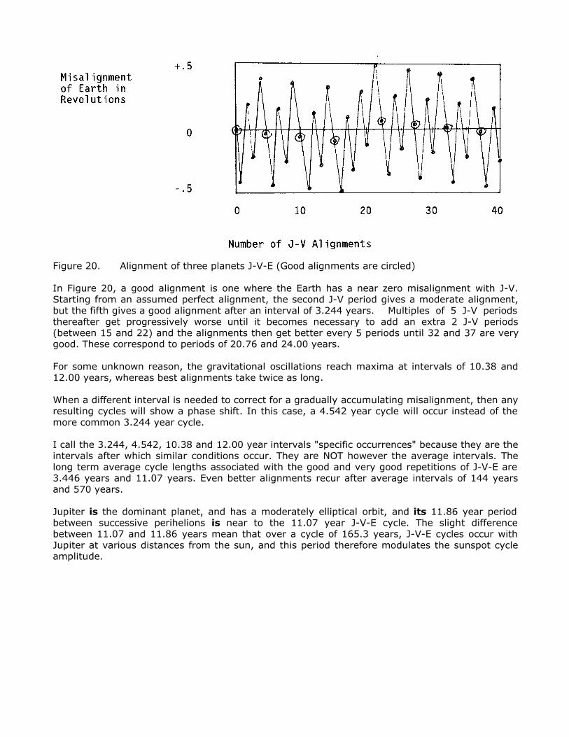
Figure 20. Alignment of three planets J-V-E (Good alignments are circled)

In Figure 20, a good alignment is one where the Earth has a near zero misalignment with J-V.Starting from an assumed perfect alignment, the second J-V period gives a moderate alignment,but the fifth gives a good alignment after an interval of 3.244 years. Multiples of 5 J-V periodsthereafter get progressively worse until it becomes necessary to add an extra 2 J-V periods(between 15 and 22) and the alignments then get better every 5 periods until 32 and 37 are verygood. These correspond to periods of 20.76 and 24.00 years.

For some unknown reason, the gravitational oscillations reach maxima at intervals of 10.38 and12.00 years, whereas best alignments take twice as long.

When a different interval is needed to correct for a gradually accumulating misalignment, then anyresulting cycles will show a phase shift. In this case, a 4.542 year cycle will occur instead of themore common 3.244 year cycle.

I call the 3.244, 4.542, 10.38 and 12.00 year intervals "specific occurrences" because they are theintervals after which similar conditions occur. They are NOT however the average intervals. Thelong term average cycle lengths associated with the good and very good repetitions of J-V-E are3.446 years and 11.07 years. Even better alignments recur after average intervals of 144 yearsand 570 years.

Jupiter is the dominant planet, and has a moderately elliptical orbit, and its 11.86 year periodbetween successive perihelions is near to the 11.07 year J-V-E cycle. The slight differencebetween 11.07 and 11.86 years mean that over a cycle of 165.3 years, J-V-E cycles occur withJupiter at various distances from the sun, and this period therefore modulates the sunspot cycleamplitude.

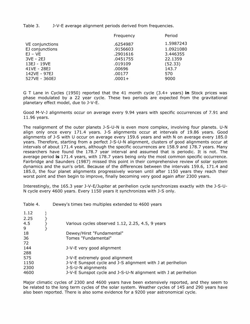
Table 3. J-V-E average alignment periods derived from frequencies.

Frequency Period

VE conjunctions .6254987 1.5987243EJ conjunctions .9156603 1.0921080EJ – VE .2901616 3.4463553VE - 2EJ .0451755 22.135913EJ - 19VE .019109 (52.33)41VE - 28EJ .00696 143.7142VE - 97EJ .00177 570527VE - 360EJ .0001+ 9000

G T Lane in Cycles (1950) reported that the 41 month cycle (3.4+ years) in Stock prices wasphase modulated by a 22 year cycle. These two periods are expected from the gravitationalplanetary effect model, due to J-V-E.

Good M-V-J alignments occur on average every 9.94 years with specific occurrences of 7.91 and11.96 years.

The realignment of the outer planets J-S-U-N is even more complex, involving four planets. U-Nalign only once every 171.4 years. J-S alignments occur at intervals of 19.86 years. Goodalignments of J-S with U occur on average every 159.6 years and with N on average every 185.0years. Therefore, starting from a perfect J-S-U-N alignment, clusters of good alignments occur atintervals of about 171.4 years, although the specific occurrences are 158.9 and 178.7 years. Manyresearchers have found the 178.7 year interval and assumed that is periodic. It is not. Theaverage period is 171.4 years, with 178.7 years being only the most common specific occurrence.Fairbridge and Saunders (1987) missed this point in their comprehensive review of solar systemdynamics and the sun's orbit. Because of the differences between the intervals 159.6, 171.4 and185.0, the four planet alignments progressively worsen until after 1150 years they reach theirworst point and then begin to improve, finally becoming very good again after 2300 years.

Interestingly, the 165.3 year J-V-E/Jupiter at perihelion cycle synchronizes exactly with the J-S-U-N cycle every 4600 years. Every 1150 years it synchronizes with J-S only.

Table 4. Dewey's times two multiples extended to 4600 years

1.12 }2.25 }4.5 } Various cycles observed 1.12, 2.25, 4.5, 9 years9 }18 Dewey/Hirst "Fundamental"36 Tomes "Fundamental"72144 J-V-E very good alignment288575 J-V-E extremely good alignment1150 J-V-E Sunspot cycle and J-S alignment with J at perihelion2300 J-S-U-N alignments4600 J-V-E Sunspot cycle and J-S-U-N alignment with J at perihelion

Major climatic cycles of 2300 and 4600 years have been extensively reported, and they seem tobe related to the long term cycles of the solar system. Weather cycles of 145 and 290 years havealso been reported. There is also some evidence for a 9200 year astronomical cycle.

The theory of harmonics put forward in this paper predicts that long period cycles will producemany harmonics especially at octaves (frequency doublings or period halvings) from the"fundamental". The above indicates that "somewhere out there" is a very long cycle working itsway down from millennia to years, months, weeks, days and even shorter periods. Remember thedaily corn prices have short periods consistent with this structure. Other researchers havereported hourly and minute cycles.

The family of cycles in table 4, although not the only one, is certainly the dominant one. In thesolar system, other families include 22.5 and 10.0 year cycles.

How long is the "fundamental" period?

I don't know, it could be the cycle of the universe; the time between big bangs.

References cited

Castle D.S. Stock Market Cycles fit the Musical Scale, Cycles, December 1956.

Dewey E.R. Cycle Frequency Harmonics, Cycles, July 1967.

Dewey E.R. Cycle Synchronies, Cycles, August 1970.

Fairbridge R.W. Article on the Sun's Orbit in Climate: History, Periodicity and Predictability.& Saunders J.E. 1987.

Gleissberg W. The Eighty-Year Sunspot Cycle, Journal of the British AstronomicalAssociation, Vol. 68, No. 4.

Hirst The Profit Magic of Transaction Timing.

Lane G.T. The 40 month cycle in Stock Prices, Cycles, 1950.

Wood Planets cause 11 year Sunspot Cycle, Nature, 1972.