1

Towards a Tractable Analysis of LocalizationFundamentals in Cellular NetworksJavier Schloemann, Member, IEEE, Harpreet S. Dhillon, Member, IEEE, and

R. Michael Buehrer, Senior Member, IEEE

Abstract—When dedicated positioning systems, such as GPS,are unavailable, a mobile device has no choice but to fallback on its cellular network for localization. Due to randomvariations in the channel conditions to its surrounding basestations (BS), the mobile device is likely to face a mix of bothfavorable and unfavorable geometries for localization. Analyticalstudies of localization performance (e.g., using the Cramer-Raolower bound) usually require that one fix the BS geometry, andfavorable geometries have always been the preferred choice inthe literature. However, not only are the resulting analyticalresults constrained to the selected geometry, this practice is likelyto lead to overly-optimistic expectations of typical localizationperformance. Ideally, localization performance should be studiedacross all possible geometric setups, thereby also removing anyselection bias. This, however, is known to be hard and hasbeen carried out only in simulation. In this paper, we developa new tractable approach where we endow the BS locationswith a distribution by modeling them as a Poisson point process(PPP), and use tools from stochastic geometry to obtain easy-to-use expressions for key performance metrics. In particular,we focus on the probability of detecting some minimum numberof BSs, which is shown to be closely coupled with a networkoperator’s ability to obtain satisfactory localization performance(e.g., meet FCC E911 requirements). This metric is indifferent tothe localization technique (e.g., TOA, TDOA, AOA, or hybridsthereof), though different techniques will presumably lead todifferent BS hearability requirements. In order to mitigateexcessive interference due to the presence of dominant interferersin the form of other BSs, we incorporate both BS coordinationand frequency reuse in the proposed framework and quantifythe resulting performance gains analytically.

Index Terms—Cellular localization, E911, hearability, stochas-tic geometry, point process theory, base station coordination,frequency reuse.

I. INTRODUCTION

GEOLOCATION (also called positioning, localization, andposition location) is deeply ingrained in our daily lives

and has been studied by the scientific community for manyyears [2]–[6]. The driving force behind much of the research isa mandate by the Federal Communications Commission (FCC)requiring cellular network operators to locate those calling 911to within certain accuracy requirements [7], [8]. Until recently,these requirements included only outdoor location accuracies.Accordingly, the predominant way cellular network operators

J. Schloemann is with Northrop Grumman Corporation, Raleigh, NC. He waswith Wireless@VT, Department of ECE, Virginia Tech, Blacksburg, VA, USA.Email: javier@vt.edu. H. S. Dhillon and R. M. Buehrer are with Wireless@VT,Department of ECE, Virginia Tech, Blacksburg, VA, USA. Email: hdhillon,buehrer@vt.edu. This paper was presented in part at the IEEE ICC 2015Workshop on Advances in Network Localization and Navigation (ANLN),London, UK [1]. Manuscript last updated: October 27, 2015.

have met the requirements of the mandate is by relying on theGlobal Positioning System (GPS). In January of 2015, however,the FCC expanded its mandate to include a phase-in of indoorpositioning requirements, citing that the bulk of emergencycalls now originate indoors [9].

While accurate outdoor positioning using GPS is reliablyavailable under clear sky conditions, many years of positioningstudy have not yet resulted in equally reliable positioningmethods in urban canyons and indoor scenarios. Considerthe classical example of locating emergency personnel (e.g.,firefighters) indoors, where our current inability to provideaccurate indoor positioning has recently been described as adilemma “where people [are] literally dying within a hundredfeet of safety” [10]. Despite this, economic limitations dictatethat global navigation satellite systems (GNSS), such asGPS, are likely to be the only widespread dedicated locationsystems in the foreseeable future. This necessitates a fallbackto terrestrial cellular networks for geolocation in situationswhere these prevalent location technologies are unavailable.Presently, however, no analytical approaches exist to study thefundamentals of localization performance in these networks.

It is the objective of this paper to introduce a newtractable model for studying terrestrial geolocation usingcellular networks. The model uses concepts from point processtheory [11] and stochastic geometry [12] to lend tractabilityto the study of network localization, which is demonstratedthrough accurate and easy-to-use expressions characterizing thenumber of base stations (BSs) that are able to participate in alocalization procedure, a key factor influencing the localizationperformance.

A. Prior art and motivation

Regardless of the technique, geolocation performance fun-damentally depends upon three things: (i) the number ofparticipating BSs, (ii) the geometry or locations of these BSsrelative to the device being localized, and (iii) the accuracy ofthe positioning observations. When these factors are determin-istic, localization performance is typically studied analyticallyusing the Cramer-Rao lower bound (CRLB) (e.g. [13]–[15]).Furthermore, since localization systems are being discussed,the topologies considered are often ones favorable to locationestimation (such as by using a carefully controlled set ofscenarios to avoid poor geometries, e.g. [14]). This approach,however, is not appropriate for studying cellular localizationperformance because none of the aforementioned factors mayreasonably be considered deterministic. Instead, the different

arX

iv:1

502.

0689

9v3

[cs

.IT

] 2

5 O

ct 2

015

2

possible locations of the mobile device within a network, thetopology of the BSs relative to the mobile device, and randomvariations in the channel conditions will (i) affect the numberof BSs capable of participating in the localization procedure,(ii) result in those BSs providing a mix of both good and badtopologies for localization, and (iii) define the strengths of thereceived BS signals which directly impact the accuracies ofthe positioning observations. Clearly, only a very large set ofdeterministic scenarios could provide insight into localizationperformance over all possible variations of the above. Even so,crafting realistic scenarios requires the assumption of specificsystem design parameters and propagation conditions, meaningthat any insights from the results would be specific to thechosen assumptions, rather than being general. This makes aclassic metric such as the CRLB not suitable for a generalanalysis.

In this work, our focus is on providing a truly general analysisof one metric which we will see is indicative of a networkoperator’s ability to meet its mandated localization accuracyrequirements–the number of successfully detectable BSs. Forcommunication, it is ideal for a mobile device to receive astrong signal from its serving BS and weak signals from all itsneighbors. For localization, on the other hand, it is increasinglybeneficial for a mobile device to receive usable signals frommore and more neighbors. Although communication is theprimary concern of network operators, cellular system designershave no choice but to also cater to localization demands. As aresult, the need to satisfy these conflicting goals has a nameamong designers–the hearability problem, due to the fact thatincreasing hearability from neighboring cells for the purposesof positioning is contrary to the principles of cellular systemdesign [16]. In order to provide a general analysis of cellularhearability, it is appropriate to characterize this metric acrossall possible network topologies and channel conditions for theaforementioned reasons.

One field of study in which random network topologies areconsidered when discussing localization is that of wireless orad-hoc sensor networks. However, these studies differ fromthe cellular scenario we consider in that the sensor networkliterature almost certainly ignores interference and propagationeffects, instead opting to define coverage using some fixeddetection range [14], [17], [18], though in rare cases thereceived signal strength may be used to define a circularcoverage region when shadowing is also considered [19].In order to apply to cellular networks, our analysis differsby not only including interference, but also by employing amodel enriched with additional cellular and localization-specificparameters.

Lastly, when cellular networks are specifically considered,they are typically studied using the popular hexagonal gridmodel, making analytical results difficult to come by. Instead,network designers resort to complex system-level simulationsusing a common set of agreed-upon evaluation parameters [20],as is clear from the 3GPP standardization process [21]. Thiscan also be seen in the limited amount of literature onhearability [22]–[24]. Though simulation-based, the work in[22] and [23] is most similar to ours in that the focus is onstudying cellular hearability (in GSM and WCDMA [22] and

LTE [23]). Interference, coordination, and fractional load areconsidered, but in the end, one is left with only simulationresults, from which it is not possible to gather general insightsinto how localization performance is impacted by system designparameters and propagation effects. This motivates the need fora tractable analytical model that can provide preliminary designinsights and will either circumvent the need for simulationscompletely or limit the ranges of the simulation parameters.In [25] and [26], such tractable, yet accurate, analytical modelswere developed to study the coverage and rate of single-tier andmulti-tier cellular communication systems, respectively. It wasshown that the spatial layout of the BSs in cellular networkscan be tractably and realistically modeled using Poisson pointprocesses (PPPs), especially as cellular networks continue todeviate from centrally-planned macro-cell networks to networkswhich include an increasing number of more arbitrary small-cell deployments such as picocells and femtocells. This opensthe door to the use of powerful tools from stochastic geometryto derive closed form expressions for key performance metrics.Motivated by these advances, we develop a similar approachto lend tractability to the analysis of localization systems.

B. ContributionsThe main contributions of this paper are as follows.A general model for studying localization in cellular networks:In Section II, we build on the foundations of [25] and [26] andpresent a tractable model specifically for studying localizationin cellular networks. The model includes average network load,the ability for BSs participating in the localization procedureto coordinate transmissions (e.g., through joint scheduling inLTE [16]), and is easily adapted to frequency reuse whenfrequency bands are assigned randomly. From [25], it is easyto see that self-interference from the network often leads topoor coverage probabilities even when the reception of only asingle signal is required. Since localization procedures requirethe successful reception of multiple signals and are thus evenmore demanding, localization systems typically necessitatethe integration of signals over time in order to improvedetectability. Our model assumes that this integration providessome fixed processing gain, while fast fading is excluded underthe assumption that it is averaged out at the receiver. Thisexclusion of small-scale fading effects in our model agreeswith the state-of-the-art 3GPP simulation models [20].Definition and characterization of accuracy-related hearabilitymetric: We define a metric in order to study the number ofBSs whose signals arrive with sufficient quality to successfullyparticipate in a localization procedure. After presenting a clearrelationship between the metric and positioning accuracy, upperbounds and approximations for the distribution of this metric arederived using the proposed model, resulting in expressions thatare closed-form in some special cases of interest, while easy-to-compute integral expressions for the others. A dominant-interferer type analysis is employed [27], [28], whereby thestrongest interference source is always treated exactly, leadingto remarkably accurate approximations, nearly indistinguishablefrom truth.Design insights: Lastly, we present results and draw out someinteresting observations useful in the design of localization

3

TABLE ISUMMARY OF KEY NOTATION

Notation Description

‖ · ‖; α `2-norm; path loss exponent (α > 2)Φ; λ PPP of BS locations; Density of Φo Origin (location of the typical user)

xi (xi) Location of the ith closest (active) BS in Φ

Ri (Ri) Distance of xi (xi) from the originγ Processing gainβ Post-processing SINR required for a successful wireless linkL Number of participating BSsp Activity factor among L participating BSsq Average network load for non-participating BSsΩ Number of participating BSs interfering with the Lth BS

b(θ, r) A ball centered at θ with radius r|A|; Ac The Lebesgue measure of region A; the complement of AB ⊆ A Region B is contained in AA\B Region A excluding its overlap with B; A\B = A ∩ Bc1(·) Indicator function; 1(A) = 1 if A is true, 0 otherwise

systems. We make evident the fact that localization performanceis limited by the interference from the BSs participating inthe localization procedure. It is shown that mitigating thisinterference through BS cooperation helps up to a point, beyondwhich the true gains in localization performance are realizedthrough frequency reuse. The need to employ frequency reusefor accurate positioning has been observed previously, but onlyby first going through the process of running many complexsystem-level simulations. In LTE, for example, a reuse of sixwas deemed necessary for downlink TDOA positioning, averdict reached after many simulations [21].

II. SYSTEM MODEL

We now formally describe the proposed model. The keynotation presented in this section is summarized in Table I.

A. Spatial base station layout

The locations of the BSs are modeled using a homogeneousPPP Φ ∈ R2 with density λ [12]. Due to the stationarity of ahomogeneous PPP, the device to be localized is assumed to belocated at the origin o. If the interference is treated as noiseat the receiver, the most appropriate metric that captures linkquality is the signal-to-interference-plus-noise ratio (SINR).For the link from some BS x ∈ Φ to the origin, the SINR canbe expressed as:

SINRx =PSx‖x‖−α∑

y∈Φy 6=x

PSy‖y‖−α + σ2, (1)

where P is the transmit power, Sz denotes the independentshadowing affecting the signal from BS z to the origin, α > 2is the pathloss exponent, and σ2 is the noise variance. Notethat (1) represents the SINR prior to any processing gain, yetas will be evident in the sequel, positioning systems typicallyhave to work at lower target SINRs, thereby necessitating theneed for some form of processing gain. In general, the post-processing SINR will include some multiplicative factor γrepresenting the processing gain, which depends upon systemparameters (e.g. integration time) and is assumed to averageout the effect of small scale fading. This is the reason why the

SINR expression in (1) does not contain a fast fading term,which is consistent with current models for evaluating cellularpositioning performance [20]. Those conversant with stochasticgeometry-based analyses of wireless networks will recognizethat the absence of fast fading on the serving link, specificallyone from the exponential family of distributions (e.g., Rayleighfading), adds to the technical challenge of a localization systemanalysis. Lastly, although we consider interference as noise,the gain from some multiuser detection technique, such asinterference cancellation, can be abstracted into the proposedmodel using the processing gain parameter γ [29].

B. Selection of participating base stations

As is common in communication system analyses, servingBSs are selected according to the strongest BS associationpolicy, measured using average signal strength, which typicallyincludes long time-scale effects such as shadowing and pathloss.Now, consider that we desire to use a total of L BSs forpositioning. Thus, we assume that the L BSs which providethe highest average received power make up the set ofparticipating BSs. Their successful participation, however, isnot guaranteed as there is some post-processing SINR thresholdβ (or equivalently, pre-processing SINR threshold β/γ) abovewhich the signals from the participating BSs must arrive inorder for them to successfully contribute to the localizationprocedure. In the absence of shadowing, the set of potentialBSs simply corresponds to the set of the L nearest BSs.When shadowing is considered and BSs are selected accordingto average signal strength, the effect of shadowing may beabsorbed as a perturbation in the locations of the BSs providedthat the fractional moment E

[S2/αz

]< ∞ [30], [31]. Thus,

when this condition is fulfilled and without loss of generality,we define a new equivalent PPP with density λE

[S2/αz

]. In

doing so, we ensure that the strongest BS association policyin the original PPP is equivalent to the nearest BS associationpolicy in the transformed PPP. For notational simplicity, wewill continue to represent the transformed PPP by Φ withdensity λ, under the assumption that if shadowing is present, itis already reflected in the density of Φ. Note that the conditionon the fractional moment is fairly mild and will almost alwaysbe satisfied by the distributions of interest, including the mostcommon assumption of log-normal shadowing with finite meanand standard deviation [31]. As a final note, it has been shownthat for SINR, shadowing causes even more regular networkmodels, such as the common hexagonal lattice, to behave likea PPP model [32]–[34]. This further validates the use of a PPPto model BS locations.

C. Base station coordination and network load

BS coordination and network load are modeled through twoactivity factors, p and q, respectively. During a localizationprocedure, the L participating BSs coordinate with each otherand attempt to blank their own transmissions while the othersare active, but are unable to do so with probability p dueto network traffic demands. The remaining BSs are assumedactive with probability q, which is simply the average network

4

Activity

factor p

Activity

factor q

RL

R1

Fig. 1. THE PROPOSED MODEL. The mobile device is denoted by the filledsquare and actively transmitting BSs are denoted by solid circles.

load [35]. For simplicity of exposition, let us order the BSsin the now shadowing-transformed Φ in terms of increasingdistance from the origin such that the location of the kth farthestBS from the origin is denoted by xk ∈ Φ. We now enrich theprevious SINR expression in (1) for the signals arriving fromthe participating BSs (i.e., xk for k ∈ 1, . . . , L) by includingBS coordination and network load as follows:

SINRk(L) =P‖xk‖−α

L∑i=1i 6=k

aiP‖xi‖−α+

∞∑j=L+1

bjP‖xj‖−α + σ2

, (2)

where ai and bj are independent indicator random variables(fixed throughout the localization procedure) modeling thethinning of the interference field by taking on value 1 withprobabilities p and q, respectively. Note that SINRk is nowa function of L because of the potentially different activityfactors for the participating BSs and the rest of the network.The number of active participating BSs interfering with theLth BS is Ω =

∑L−1i=1 ai, which is a binomial random variable

with probability mass function

fΩ(ω) =

(L− 1

ω

)pω(1− p)L−1−ω, ω ∈ 0, . . . , L− 1.

(3)

D. Base station range distributions

From (2), it is clear that the SINRs are dependent on thedistances of the BSs from the origin, rather than the locationsthemselves. Thus, it is worthwhile to characterize these. LetRk = ‖xk‖ and Rm = ‖xm‖, where xm is now the mth

farthest active BS. This is illustrated in Figure 1 for the closestactive (R1) and Lth closest overall (RL) BSs. The distributionof RL is [36]:

fRL(r) = e−λπr2 2(λπr2)L

r(L− 1)!. (4)

Now, conditioned on Ω and the distance of the Lth BS fromorigin, we present a useful lemma for understanding thedistribution of the locations of the Ω active participating BSs.

Lemma 1. Conditioned on the distance of the Lth BS from theorigin, RL, the Ω active BSs closer to the origin than the Lth

BS are independent and identically distributed over b(o,RL)with the location of each BS sampled uniformly at randomfrom b(o,RL).

Proof: See Appendix A.Note that a point process is which a fixed number of points

are distributed uniformly at random independent of each otherin a given compact set is termed as a uniform Binomial PointProcess (BPP) [12]. Therefore, the above Lemma simply statesthat conditioned on RL, Ω active BSs closer to the origin thanthe Lth BS form a BPP on b(o,RL).Using Lemma 1, we obtain the following distribution for themost dominant (i.e., closest active) interferer, given the distanceof the Lth BS and Ω. This is formally presented below.

Lemma 2. The cumulative distribution function of the closestactive BS distance R1 given RL and Ω is

FR1|RL,Ω(r|RL,Ω) = 1−(R2L − r2

R2L

)Ω

, 0 ≤ r ≤ RL. (5)

Proof: See Appendix B.Let A = b(o,RL)\b(o, R1), where b(θ, r) represents a ballof radius r centered at θ. We have the following lemmacharacterizing the distribution of the Ω− 1 remaining activeBSs in the annular region A.

Lemma 3. Conditioned on R1 and RL, the Ω − 1 activeBSs located inside the annular region b(o,RL)\b(o, R1) aredistributed according to a uniform BPP.

Proof: See Appendix A.

III. LOCALIZATION PERFORMANCE

As mentioned in Section I, localization performance funda-mentally depends on the number of positioning observations,their accuracies, and the locations of the participating BSsrelative to the device being localized. These three factors areall highly interdependent. For instance, both the number of BSswhose signals arrive with sufficiently-high SINRs to participatein the localization procedure and the quality of their positioningobservations are strongly dependent on the interference field,which is itself driven by the realized network deployment.Thus, a full characterization of localization performance wouldtake into account all possible geometric conditionings of theBSs over all possible channel conditions, a task which isextremely difficult. By taking into account even just the numberof participating BSs averaged over the channel conditions,however, valuable insights into localization performance maybe gleaned.

A. Base station participation and geolocation performance

A clear relationship exists between the number of BSsinvolved in positioning and a cellular network operator’s ability

5

0 20 40 60 80 100 120 140 1600

0.1

0.2

0.3

0.4

0.5

0.6

0.7

0.8

0.9

1

Positioning error (m)

P(P

ositio

nin

g e

rro

r ≤ A

bscis

sa

)

L ≥ 1

L ≥ 2

L ≥ 3

L ≥ 4

L ≥ 5

L ≥ 6

L ≥ 7

L ≥ 8

L ≥ 9

Fig. 2. IMPACT OF BS PARTICIPATION ON MEETING FCC E911 REQUIRE-MENTS: Positioning performance of an OTDOA-like system with settingsderived from [38] (see text). A performance curve must pass through bothhorizontal dashed lines in order to meet the FCC mandate.

to meet its geolocation performance requirements [21]. In orderto see this, consider handset-based TDOA positioning, such asObserved Time-Difference-Of-Arrival or OTDOA in LTE. TheFCC E911 mandate requires that operators employing handset-based localization estimate the locations of mobile devices towithin an accuracy of 50 m 67% of the time and 150 m 90%of the time [37]. Using the model described in the previoussection with a BS deployment density equivalent to that ofan infinite hexagonal grid with 500 m intersite distances, ashadowing standard deviation of 8 dB, and a pathloss exponentof α = 3.76, an example localization system was simulatedrequiring a pre-processing SINR β/γ = −13 dB for successfulsignal detection [38]. A fully-loaded network was assumed withno BS coordination (i.e., p = q = 1) and clock inaccuracies ateach BS modeled normally with a standard deviation of 100 ns.The SINR threshold determines which BSs may successfullyparticipate in the localization procedure, while an individualranging observation is modeled as the sum of an exponentially-distributed non-line-of-sight bias with a mean of 30 m and azero-mean Gaussian random variable with a variance basedon the exact SINR and calculated using the well-known TOAranging CRLB [39] using a signal bandwidth of 10 MHz. Lastly,positions were estimated using the algorithm presented in [5]with the strongest BS selected as the reference BS. The resultinglocalization performance is shown in Figure 2 for severalminimum BS hearabilities. From this particular example, anetwork operator might conclude that, with universal frequencyreuse on the positioning signals, a hearability of 6 BSs wouldbe required to be in compliance with the requirements of theFCC E911 mandate.

Motivated by this connection, we now formally proposea metric to study the number of BSs able to successfullyparticipate in a localization procedure for a given target SINRβ and processing gain γ.

Definition 1 (Participation metric). For a given BS deploymentφ ∈ Φ, let Υ represent the maximum number of selectable BSs

such that all successfully participate in a localization procedure.This can be mathematically defined as:

Υ = arg max`

`×∏k=1

1

(SINRk(`) ≥ β

γ

). (6)

Note that this metric differs from a traditional metric such asthe CRLB in that it is not directly tied to a specific positioningaccuracy value, though it is still closely related. Its advantagelies in its tractability when characterized over all the possibleBS topologies, whereas the CRLB, on the other hand, doesprovide direct insight into achievable positioning accuracy, butonly for deterministic networks, quickly becoming intractableto characterize over all BS topologies.

B. Participation from a desired number of base stations

While generally better localization performance can beattained by increasing BS participation, the probability ofobtaining some desired number of successful BS connections isknown to decrease sharply as the number increases. How thisfundamental factor influencing localization system performancechanges across different parameter sets is exactly the objectiveof our study. Thus, it is desirable to understand exactly how Υis impacted by the network design parameters and propagationeffects, averaged over the geometric conditions and channelvariations.

Definition 2 (L-localizability probability). For a given φ ∈ Φ,a mobile device is said to be L-localizable if at least L BSsmay successfully participate in the localization procedure. Theprobability of this occurring is simply:

PL = P (Υ ≥ L) = E

[L∏k=1

1

(SINRk(L) ≥ β

γ

)]. (7)

It may be insightful to step back and consider a specificapplication of PL. Note that the first objective in any locationsystem is to make sure that the device to be located can detectpositioning signals from a sufficient number of BSs (i.e., thatit is localizable). By this, we simply mean that an estimate ofthe device’s location can be found without ambiguity. In thenoiseless case, this means that there can only be one solution. Inthe noisy case, this means that there is a single global minimumto the appropriate cost function. Commonly-accepted minimumvalues of L for the unambiguous operation of a localizationsystem in the R2 plane are 2, 3, and 4 for AOA, TOA/RSS, andTDOA, respectively. Thus, for example, P4 can be equivalentlythought of as the coverage probability of TDOA positioning.

For two edge cases of interest, that with no BS coordination(p = 1) and that with perfect BS coordination (p = 0), it isstraightforward to infer from (2) that

1 (SINRk(L) ≥ β) ≥ 1 (SINRl(L) ≥ β) (8)

for all k ≤ l ≤ L. This simply means that the received SINRfrom a BS farther from the mobile device is lower than that ofa closer BS, implying that the probability of L-localizabilityin (7) can be equivalently expressed as

PL = E [1 (SINRL(L) ≥ β/γ)] . (9)

6

Fig. 3. LOWER BOUNDING THE INTERFERENCE: As in Figure 1, trans-mitting/quiet BSs are denoted by filled/hollow circles and the device to belocalized is denoted by the filled square.

With partial BS coordination (0 < p < 1), the relationship in(8) does not hold in certain corner cases. These rare occurrenceshave a minimal impact on our analysis, and we proceed by usingthe expression for PL in (9) for all p. In the numerical results,we will validate that (9) is in fact an accurate approximationof PL for all p by comparing with the true PL, which jointlyconsiders the SINRs of all participating BSs.

C. A simple bound on PL

We now derive an upper bound on L-coverage probabilityby (i) considering the closest interferer’s location exactly, (ii)placing the remaining Ω−1 active interior interferers at the edgeof the field of participating BSs, and (iii) ignoring thermal noiseand all distant BSs. We illustrate this setup in Figure 3, whichapplies the above considerations to the network realization ofFigure 1. Note that the interference from all BSs beyond theLth BS is ignored, while the active interior BSs have beenpushed out to the same distance as the Lth BS. The dominantinterferer, however, has been left untouched.

Theorem 1 (Upper bound on L-coverage probability). Theprobability that a device can successfully utilize a desired LBSs for positioning is upper bounded by

PL(p, q, α, β, γ, λ) ≤χ∑ω=0

(1−

(γ

β− (ω − 1)

)− 2α

)ωfΩ(ω),

(10)

where χ = minL− 1, bγ/βc.

Proof: See Appendix C.One thing we notice immediately from (10) is that the boundis independent from the BS deployment density λ. This isin line with similar observations made in coverage analysesfor interference-limited networks (i.e., network interferencedominates thermal noise) [25], [26]. We will return to thisobservation at the end of this section. In the special case when

all participating BSs transmit simultaneously, the above boundreduces to a simple closed-form expression.

Corollary 1.1 (The special case of p = 1). When allparticipating BSs transmit simultaneously,

PL(1, 1, α, β, γ, λ) ≤

(1−

(γ

β− (L− 2)

)− 2α

)L−1

, (11)

for β < γL−1 , and zero otherwise.

Proof: When p = 1, fΩ(L−1) = 1 and the result followsfrom (10).From this result, we see that as greater numbers of participatingBSs are desired, the probability of attaining those numbers ofBSs with sufficiently strong connections decreases dramatically.Note that by rearranging (11), we also obtain a useful lowerbound on the processing gain required to achieve some desiredL-localizabity probability.

Corollary 1.2 (Lower bound on processing gain with no BScoordination). The processing gain required to reach a desiredL-coverage probability PL when p = 1 is lower-bounded by

γ ≥ β((

1− PL1

L−1

)−α2+ L− 2

). (12)

D. Approximations of PL

Let

I1 =

Ω∑i=2

P‖xi‖−α (13)

be the aggregate interference due to the active BSs (if any)between x1 and xL. Furthermore, let

I2 =

∞∑j=L+1

bjP‖xj‖−α (14)

be the aggregate interference due to the infinite field of BSslocated further than the Lth BS. Clearly then, when Ω ≥ 1,

SINRL(L) =PR−αL

PR−α1 + I1 + I2 + σ2. (15)

In this section, we will approximate (15) and in turn PL bymaking the following assumption.

Assumption 1. We assume that if the dominant interferer(i.e., the closest active BS) is considered exactly, the remaininginterference terms in (15), namely I1 and I2, may be accuratelyapproximated by their means conditioned on R1, RL, and Ω.

This type of dominant interferer analysis has been employedpreviously with desirable results [27], [28] and will yieldremarkably simple, yet accurate, approximations in our analysis,as will be demonstrated later. This is because considering R1

exactly and I1 using its mean (conditioned on R1), results inan accurate approximation of the total interference due to theBSs closer than xL, which is typically the performance-limitingterm.

7

In interference-limited networks, Assumption 1 allows us toreplace SINRL(L) in (9) by

SIRL(L) =PR−αL

PR−α1 + E[I1|R1, RL,Ω] + E[I2|RL], (16)

where SIR stands for the signal-to-interference ratio. As thedeployment density grows, the assumption of interference-limited networks increases in validity, and since our workis motivated by the reuse of existing infrastructures, suchas cellular networks with small cell extensions which haverelatively high deployment densities, we aver that it is quitereasonable. Expressions for the above conditional means arepresented in the following lemmas.

Lemma 4. The expected value of I1 conditioned on R1, RL,and Ω is

E[I1|R1, RL,Ω] =2P (Ω− 1)

2− α·R2−αL − R2−α

1

R2L − R2

1

, (17)

for Ω ≥ 1, and zero otherwise.

Proof: See Appendix D.

Lemma 5. The expected value of I2 conditioned on RL is

E[I2|RL] =2Pπqλ

α− 2R2−αL , (18)

for α > 2, and unbounded otherwise.

Proof: See Appendix E.By inserting the results of Lemmas 4 and 5 into (16), we obtainincreasingly specialized (and simpler) approximations of theL-localizability probability. In order to proceed, however, wemust first account for the case when Ω = 0, in which case R1 in(16) has no meaning. Thus, we first derive an approximation ofPL for the special Ω = 0 case, which incidentally correspondsto the perfect coordination (p = 0) scenario.

Proposition 1. Under Assumption 1, the probability of L-localizability with perfect BS coordination in interference-limited networks is

PL(0, q, α, β, γ, λ) = 1−L−1∑`=0

e−α−2

2qβ/γ

(α−2

2qβ/γ

)``!

. (19)

Proof: See Appendix F.As noted in the proof of above Proposition, (19) can beinterpreted as the probability that at least L BSs (modeled bya PPP) lie inside b

(o,√

α−22πqλβ/γ

). Moreover, note that the

density of the BS deployment does not appear to affect PL.With this special case out of the way, we now proceed, startingwith our most general result.

Theorem 2. Under Assumption 1, the probability that a mobiledevice is able to localize itself using L BSs in interference-limited networks is PL(p, q, α, β, γ, λ) =1−

L−1∑`=0

e−α−2

2qβ/γ

(α−2

2qβ/γ

)``!

fΩ(0) +4(λπ)L

(L− 1)!

L−1∑ω=1

fΩ(ω)

∫ ∞0

∫ rL

0

1

r−αL

r−α1 + 2(ω−1)2−α ·

r2−αL −r2−α

1

r2L−r2

1+ 2πqλ

α−2 r2−αL

≥ β

γ

r1(r2

L − r21)ω−1r

2(L−ω)−1L ωe−λπr

2L dr1 drL. (20)

Proof: See Appendix G.Thus, we obtain an expression which requires only doubleintegration in order to determine PL, and though the outsideintegral has an infinite integration bound, the expression isnot difficult to evaluate numerically thanks to the decayingexponential term in the integrand. To appreciate the valueof this approximation, consider the p = 1 scenario in whichcase the first term in (20) disappears and the summand needonly be evaluated at ω = L − 1. Though the authors didnot have localization in mind, the exact expression for thek-coverage problem in the absence of fast fading in [40, Corr.7] applies directly to PL for p = q = 1. A cursory glance atthe exact expression in [40] reveals its cumbersome nature,involving sums over many multi-fold integrals even in theabsence of thermal noise, which is considerably more complexin comparison to (20). Moreover, by applying a slight secondaryapproximation and multiplying E[I2|RL] in (16) by E[R2

1]/R21,

where E[R21] = 1

πλ [36], (20) is further reduced, yielding asingle-integral expression applicable to the general case.

Corollary 2.1. The general expression for PL in (20) maybe further (and consequently, less reliably) approximated forinterference-limited networks by: PL(p, q, α, β, γ, λ) =

PL(0, q, α, β, γ, λ)fΩ(0) + 2

L−1∑ω=1

fΩ(ω)ω

∫ ∞1

1

(xα+

2(ω − 1)

2− α· x

2 − xα

x2 − 1+

2qx2

α− 2≤ γ

β

)(1− x−2

)ω−1

x3dx. (21)

Proof: See Appendix H.This expression is instantly and accurately evaluated in anumerical computation environment such as MATLAB. We nowbriefly describe how the introduction of the additional termsinto (16) reduces (20). The key is that after some algebraicmanipulation, (16) may now be expressed as follows (see (31)in the appendix): SIRL(L) ≈

1(RLR1

)α+ 2(Ω−1)

2−α ·(RLR1

)2−(RLR1

)α(RLR1

)2−1

+ 2qα−2

(RLR1

)2, (22)

which contains R1 and RL only through their ratio X =RL/R1. The cumulative distribution function of this ratioadmits the simple form of FX(x) = (1 − 1/x2)Ω, whichis readily obtained from (5). For the special case of α = 4,this additional approximation needn’t be used, however, as asingle integral expression is obtained directly from (20).

Corollary 2.2. Under Assumption 1 and for the special caseof α = 4 in interference-limited networks,

PL(p, q, 4, β, γ, λ) =

χ∑ω=0

fΩ(ω)

∫ √γ/β−ωπqλ

0

8

1− 1√γ/β − πqλr2 + (ω−1)2

4 − ω−12

ω

fRL(r)dr, (23)

where χ = minL− 1, bγ/βc.

Proof: See Appendix I.For fully-loaded networks (i.e., p = q = 1), (23) simplifiesfurther to the following expression.

Corollary 2.3. Under Assumption 1 and for the special caseof α = 4 in fully-loaded interference-limited networks,

PL(1, 1, 4, β, γ, λ) =

∫ √γ/β−(L−1)

πλ

01− 1√γ/β − πλr2 + (L−2)2

4 − L−22

L−1

fRL(r)dr,

(24)

for β < γL−1 and zero otherwise.

For larger values of L and higher values of p, it may bereasonable to ignore the I2 term in (16) under the assumptionthat the interference due to the Ω active participating BSsdominates that of the rest of the network. By doing so,expressions not requiring any integration may be found for thespecial cases covered in Corollaries 2.2 and 2.3.

Corollary 2.4. Under Assumption 1, α = 4, PL for networkslimited by the interference from the nearby BSs participatingin the localization procedure is PL(p, q, 4, β, γ, λ) =

χ∑ω=0

fΩ(ω)

1− 1√γ/β + (ω−1)2

4 − ω−12

ω

, (25)

where χ = minL− 1, bγ/βc.

Proof: Consider the limit of (23) as q → 0. Theparenthetical term becomes independent of r and may bepulled out of the integral, while the remaining integral coversthe probability density function fRL(r) over the entirety of itsdomain, thus evaluating to 1.

Corollary 2.5. Under Assumption 1 and when α = 4, PLfor fully-loaded networks limited by the interference from thenearby BSs participating in the localization procedure is

PL(1, 1, 4, β, γ, λ) =

1− 1√γ/β + (L−2)2

4 − L−22

L−1

,

(26)for β < γ

L−1 and zero otherwise.

Interestingly, when interference from the participating BSs isignored in (19) and when distant network interference is ignoredin (25) and (26), the resulting expressions are independent ofthe BS deployment density. This is termed as scale invariancein the literature and is known to hold for most of the metricsthat are derived from SINR when the thermal noise is negligibleor ignored (interference-limited scenarios), e.g., see [25], [26].

IV. NUMERICAL RESULTS AND DISCUSSION

We now study the tightness of the bound and the approxi-mations, as well as gather insights from numerical results. Forconsistency, all results were gathered using a BS deploymentdensity equivalent to that of an infinite hexagonal grid with500 m intersite distances (i.e., λ = 2/(

√3 · 5002 m2)) and a

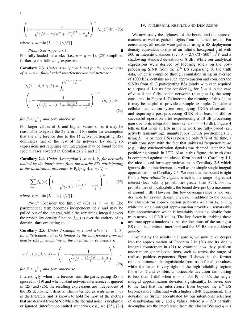
shadowing standard deviation of 8 dB. While our analyticalexpressions were derived by focusing solely on the post-processing SINR from the Lth BS surpassing β, the truthdata, which is compiled through simulation using an averageof 1000 BSs, contains no such approximation and considers theSINRs from all L participating BSs jointly with each requiredto surpass β. Let us first consider PL for L = 4 in the caseof α = 4 and fully-loaded networks (p = q = 1), the setupconsidered in Figure 4. To interpret the meaning of this figure,it may be helpful to provide a simple example. Consider acellular localization system employing TDOA observationsand requiring a post-processing SINR of at least −6 dB forsuccessful operation after experiencing a 10 dB processinggain due to its integration time (i.e. β/γ = −16 dB). Figure 4tells us that when all BSs in the network are fully-loaded (i.e.,actively transmitting), unambiguous TDOA positioning (i.e.,using L = 4 or more BSs) is possible only 50% of the time, aresult consistent with the fact that universal frequency reuse(e.g., using synchronization signals) was deemed untenable forpositioning signals in LTE. Also in this figure, the truth datais compared against the closed-form bound in Corollary 1.1,the nice closed-form approximation in Corollary 2.5 whichignores distant interference, as well as the simple single-integralapproximation in Corollary 2.3. We note that the bound is tightfor the high-reliability regime, which is the range of greatestinterest (localizability probabilities greater than 0.75). For lowprobabilities of localizability, the bound diverges by a maximumof around 3 dB. However, this low coverage range is not verydesirable for system design, anyway. In addition to the bound,the closed-form approximation performs well for PL > 0.6,while the single-integral approximation provides a remarkablytight approximation which is invariably indistinguishable fromtruth across all SINR values. The key factor in enabling theseaccurate approximations is that the locations of the strongestBS (i.e., the dominant interferer) and the Lth BS are consideredexactly.

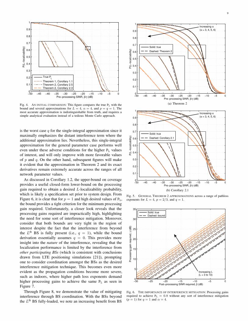
Inspired by the results in Figure 4, we now delve deeperinto the approximation of Theorem 2 in (20) and its single-integral counterpart in (21) to examine how they performunder more general conditions, such as across the range ofrealistic pathloss exponents. Figure 5 shows that the formerremains almost indistinguishable from truth for all α values,while the latter is very tight in the high-reliability regimefor α > 3 and exhibits a noticeable deviation (amountingto less than 1 dB) when α = 3. For PL < 0.5, the single-integral approximation deviates significantly, however, dueto the fact that the interference from beyond the Lth BSbecomes more influential with a higher SINR requirement. Thisdeviation is further accentuated by our intentional selectionof disadvantageous p and q values, where p = 2/3 partiallyde-emphasizes the interference from the closest BSs and q = 1

9

−50 −45 −40 −35 −30 −25 −20 −15 −10 −5 00

0.1

0.2

0.3

0.4

0.5

0.6

0.7

0.8

0.9

1

Pre−processing SINR, β/γ (dB)

P(L

−lo

caliz

abili

ty)

True PL

Theorem 1, Corollary 1.1

Theorem 2, Corollary 2.5

Theorem 2, Corollary 2.3

Fig. 4. AN INITIAL COMPARISON: This figure compares the true PL with thebound and several approximations for L = 4, α = 4, and p = q = 1. Themost accurate approximation is indistinguishable from truth, and requires asimple analytical evaluation instead of a tedious Monte Carlo approach.

is the worst case q for the single-integral approximation since itmaximally emphasizes the distant interference term where theadditional approximation lies. Nevertheless, this single-integralapproximation for the general parameter case performs welleven under these adverse conditions for the higher PL valuesof interest, and will only improve with more favorable valuesof p and q. On the other hand, subsequent figures will makeit evident that the approximation in Theorem 2 and its exactderivatives remain extremely accurate across the ranges of allnetwork parameter values.

As discussed in Corollary 1.2, the upper-bound on coverageprovides a useful closed-form lower-bound on the processinggain required to obtain a desired L-localizability probability,which is likely a specification set prior to system design. FromFigure 6, it is clear that for p = 1 and high desired values of PL,the bound provides a tight criterion for the minimum processinggain required. Unfortunately, a closer look reveals that theprocessing gains required are impractically high, highlightingthe need for some sort of interference mitigation. Moreover,consider that both bounds are very tight in the region ofinterest despite the fact that the interference from beyondthe Lth BS is fully present (i.e., q = 1), while the boundderivation essentially assumes q = 0. This provides moreinsight into the nature of the interference, revealing that thelocalization performance is limited by the interference fromother participating BSs (which is consistent with conclusionsdrawn from LTE positioning simulations [21]), promptingone to consider coordination amongst the BSs as the desiredinterference mitigation technique. This becomes even moreevident as the propagation conditions become more severe,such as indoors, where higher path loss exponents demandhigher processing gains to achieve the same PL as seen inFigure 7.

Through Figure 8, we demonstrate the value of mitigatinginterference through BS coordination. With the BSs beyondthe Lth BS fully-loaded, we note an increasing benefit from BS

−50 −45 −40 −35 −30 −25 −20 −15 −10 −5 00

0.1

0.2

0.3

0.4

0.5

0.6

0.7

0.8

0.9

1

Pre−processing SINR, β/γ (dB)

P(L

−lo

caliz

abili

ty)

Solid: true

Dashed: Theorem 2

Increasing α

(α = 3, 4, 5, 6)

(a) Theorem 2

−50 −45 −40 −35 −30 −25 −20 −15 −10 −5 00

0.1

0.2

0.3

0.4

0.5

0.6

0.7

0.8

0.9

1

Pre−processing SINR, β/γ (dB)

P(L

−lo

caliz

abili

ty)

Solid: true

Dashed: Corollary 2.1

Increasing α

(α = 3, 4, 5, 6)

(b) Corollary 2.1

Fig. 5. GENERAL THEOREM 2 APPROXIMATIONS across a range of pathlossexponents for L = 4, p = 2/3, and q = 1.

−30 −25 −20 −15 −10 −5 00

5

10

15

20

25

30

35

Post−processing SINR required, β (dB)

Pro

ce

ssin

g g

ain

re

qu

ire

d,

γ (d

B)

Solid: true

Dashed: bound

Increasing L(L = 3 to 10)

Fig. 6. THE IMPORTANCE OF INTERFERENCE MITIGATION: Processing gainsrequired to achieve PL = 0.8 without any sort of interference mitigation(p = 1) for q = 1 and α = 4.

10

−30 −25 −20 −15 −10 −5 00

5

10

15

20

25

30

35

Post−processing SINR required, β (dB)

Pro

ce

ssin

g g

ain

re

qu

ire

d,

γ (d

B)

Solid: true

Dashed: bound

Increasing α

(α = 3, 3.5, …, 6)

Fig. 7. THE IMPACT OF PATH LOSS: Processing gains required for desiredPL values grow exponentially with the pathloss exponent. (PL = 0.8, L = 4,p = q = 1.)

−50 −45 −40 −35 −30 −25 −20 −15 −10 −5 00

0.1

0.2

0.3

0.4

0.5

0.6

0.7

0.8

0.9

1

Pre−processing SINR, β/γ (dB)

P(L

−lo

caliz

abili

ty)

Solid: true

Dashed: Theorem 2

Increasingcoordination

(p = 1, 0.9, …, 0)

Fig. 8. THE BENEFIT OF BS COORDINATION: These L-localizabilityprobabilities emphasize the gains achievable through the coordinated mitigationof participating BS interference. (L = 4, α = 4, q = 1.)

coordination as the degree of the coordination is incrementallyincreased. The large improvement in hearability from p = 1 top = 0 again sheds light on the issue of interference from nearbyBSs. In fact, at its least detrimental point, the interference fromthe L − 1 closest BSs accounts for nearly a 10 dB drop insignal quality. That’s roughly the equivalent of going fromsuccessfully obtaining eleven to obtaining only four BSs in thenetwork considered in Figure 9. While coordination is able tohelp significantly, a closer look at Figures 8 and 9 makes itclear that more is necessary in order to reach the truly highL-localizability probabilities at reasonable SINR values. Themost prevalent technique to further reduce the interference isthat of thinning the interference field by separating nearbytransmitters in frequency, which is discussed next.

−50 −45 −40 −35 −30 −25 −20 −15 −10 −5 00

0.1

0.2

0.3

0.4

0.5

0.6

0.7

0.8

0.9

1

Pre−processing SINR, β/γ (dB)

P(L

−lo

caliz

abili

ty)

Solid: true

Dashed: Theorem 2

Increasing L(L = 3 to 11)

Fig. 9. THE COST OF INVOLVING MORE BSS: This figure underscores thehigh cost of obtaining a greater desired number of BSs, particularly in thehigh-reliability regime. (α = 4, p = 1/2, q = 3/4.)

A. Application to frequency reuse

An effective technique to reduce interference from co-locatedtransmitters is that of frequency reuse, commonly included inwireless standards [41]. If a total of K frequency bands areavailable and we independently assign one of the bands toeach x ∈ Φ with equal probability, we can easily incorporatefrequency reuse into our model by considering the transmissionactivity on each band separately using independent PPPs whosedensities are that of the original PPP thinned by the frequencyreuse factor K. Let us denote the number of detectable BSsin the kth band by nk. For L-localizability, we thus require∑Kk=1 nk ≥ L. The main technical difference between this

analysis and that already presented is that we are now obligedto evaluate the probability of being able to detect exactly nBSs in a given frequency band. Under the localization setup weconsider, it is not difficult to show that when p = q this can bereadily determined by considering the difference between theprobabilities of n and n+ 1 localizability. The p = q conditionisn’t particularly restrictive, as it still allows us to model averagenetwork load and only removes the ability to perform per-band BS coordination (which isn’t done in practice, anyway).From here, the expression for the L-localizability probabilitywith frequency reuse is procured by simply considering allcombinations of n1, . . . , nK for which

∑Kk=1 nk ≥ L. This

is formally stated in the following theorem.

Theorem 3 (L-localizability probability with random frequencyreuse). The L-localizability probability with random frequencyreuse and reuse factor K is:

PKL(p, q, α, β, γ, λ) = 1−L−1∑l=0

∑n1,...,nK∑

i ni=l

K∏i=1(

Pni

(p, q, α, β, γ,

λ

K

)− Pni+1

(p, q, α, β, γ,

λ

K

)).

(27)

This expression is easily implemented in software using a

11

−30 −25 −20 −15 −10 −5 0 5 10 15 200

0.1

0.2

0.3

0.4

0.5

0.6

0.7

0.8

0.9

1

Pre−processing SINR, β/γ (dB)

P(L

−lo

ca

liza

bili

ty)

Solid: true

Dashed: Theorem 2

Increasingfrequency reuse(K = 1, 2, 3, 6)

Fig. 10. THE VALUE OF FREQUENCY REUSE is undeniable for improving PL.Here, L = 4, α = 4, p = q = 1.

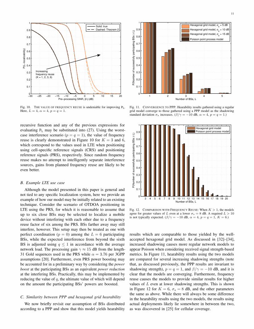
recursive function and any of the previous expressions forevaluating PL may be substituted into (27). Using the worst-case interference scenario (p = q = 1), the value of frequencyreuse is clearly demonstrated in Figure 10 for K = 3 and 6,which correspond to the values used in LTE when positioningusing cell-specific reference signals (CRS) and positioningreference signals (PRS), respectively. Since random frequencyreuse makes no attempt to intelligently separate interferencesources, gains from planned frequency reuse are likely to beeven better.

B. Example LTE use case

Although the model presented in this paper is general andnot tied to any specific localization system, here we provide anexample of how our model may be initially related to an existingtechnique. Consider the scenario of OTDOA positioning inLTE using the PRS, for which it is reasonable to assume thatup to six close BSs may be selected to localize a mobiledevice without interfering with each other due to a frequencyreuse factor of six among the PRS. BSs farther away may stillinterfere, however. This setup may then be treated as one withperfect coordination (p = 0) among the L = 6 participatingBSs, while the expected interference from beyond the sixthBS is adjusted using q ≤ 1 in accordance with the averagenetwork load. The processing gain γ ≈ 15 dB from the length-31 Gold sequences used in the PRS while α = 3.76 per 3GPPassumptions [20]. Furthermore, even PRS power boosting maybe accounted for in a preliminary way by considering the powerboost at the participating BSs as an equivalent power reductionat the interfering BSs. Practically, this may be implemented byreducing the value of q, the ultimate value of which will dependon the amount the participating BSs’ powers are boosted.

C. Similarity between PPP and hexagonal grid hearability

We now briefly revisit our assumption of BSs distributedaccording to a PPP and show that this model yields hearability

1 2 3 4 50

0.1

0.2

0.3

0.4

0.5

0.6

0.7

0.8

0.9

1

Number of BSs, L

P(N

um

ber

of successfu

lly p

art

icip

ating B

Ss ≥

L)

Hexagonal grid model, σ

s = 5 dB

Hexagonal grid model, σs = 10 dB

Hexagonal grid model, σs = 15 dB

Poisson point process model

Fig. 11. CONVERGENCE TO PPP: Hearability results gathered using a regulargrid model converge to those gathered using a PPP model as the shadowingstandard deviation σs increases. (β/γ = −10 dB, α = 4, p = q = 1.)

3 4 5 6 7 8 9 10 11 12 13 14 15 16 17 18 19 200

0.1

0.2

0.3

0.4

0.5

0.6

0.7

0.8

0.9

1

Number of BSs, L

P(N

um

ber

of successfu

lly p

art

icip

ating B

Ss ≥

L)

Hexagonal grid model

Poisson point process model

Fig. 12. COMPARISON WITH FREQUENCY REUSE: When K > 1, the modelsagree for greater values of L even at a lower σs = 8 dB. A required L > 10is not typically expected. (β/γ = −10 dB, α = 4, p = q = 1, K = 6.)

results which are comparable to those yielded by the well-accepted hexagonal grid model. As discussed in [32]–[34],increased shadowing causes more regular network models toappear Poisson when considering received signal strength-basedmetrics. In Figure 11, hearability results using the two modelsare compared for several increasing shadowing strengths (notethat, as discussed previously, the PPP results are invariant toshadowing strength), p = q = 1, and β/γ = −10 dB, and it isclear that the models are converging. Furthermore, frequencyreuse causes the models to provide similar results for highervalues of L even at lower shadowing strengths. This is shownin Figure 12 for K = 6, σs = 8 dB, and the other parametersthe same as above. While there will always be some differencein the hearability results using the two models, the results usingactual deployments likely lie somewhere in between the two,as was discovered in [25] for cellular coverage.

12

V. CONCLUSION

We have employed concepts from point process theory andstochastic geometry in order to provide a new tractable modelfor studying localization in cellular networks. The model isaccompanied by an analysis of hearability, which is shownto be an important metric providing insight into fundamentallocalization performance, and easy-to-use analytical expressionsfor this metric are provided. This is in contrast to mostprevious approaches, which either provide insights specificto deterministic deployments or rely on time-consumingsimulations, neither of which allow for the drawing of generalinsights. While more base stations participating in localizationis beneficial to its accuracy, the analytical results show thatobtaining an increasing number of successful base stationsconnections decreases exponentially. The primary culprit forthis is the interference due to the participating base stationsthemselves. When base stations coordinate (e.g., through anetwork controller), more of them are able to successfullyparticipate in the localization procedure. However, in the end,it is clear that the greatest gains in hearability are realizedthrough frequency reuse. This is consistent with the findingsduring the standardization of LTE positioning, where thisconclusion was reached after performing many complex system-level simulations.

We have only scratched the surface of the model, whichmay be used to extend this work in many different ways.Besides hearability, understanding how other metrics, such asones focused on network geometry, are affected by changesin design parameters would yield valuable contributions to thelocalization literature. In addition, recognizing how directionalantennas and power control affect localization performancewould be helpful to cellular system designers. Lastly, locationinformation can be gathered in diverse ways, for example bysimply knowing that one is able to hear a low-power femtocell,which lends itself nicely to the consideration of differentclasses of base stations through multi-tiered heterogeneousnetworks [26].

APPENDIX

A. Proof of Lemmas 1 and 3

The proof strategy used here is quite standard, e.g., see [12,Theorem 2.9]. For the proof, let i < j, n ≤ ℵ, ℵ bethe number of BSs between xi and xj , A = b(o, ‖xi‖ +δ/2)\b(o, ‖xi‖−δ/2), B = b(o, ‖xj‖+ε/2)\b(o, ‖xj‖−ε/2),C = b(o, ‖xj‖ − ε/2)\b(o, ‖xi‖ + δ/2), D ⊆ C, b(θ, r)represent a ball of radius r centered at θ, δ and ε be smallmodifications to the regions of A, B, and C, and NH be thenumber of points in region H. Then, P(ND = n|xi, xj) =

limδ,ε→0

P(ND = n|NC = ℵ, NB = 1, NA = 1)

= limδ,ε→0

P(ND = n,NC = ℵ, NB = 1, NA = 1)

P(NC = ℵ, NB = 1, NA = 1)

= limδ,ε→0

P(ND = n,NC\D = ℵ − n,NB = 1, NA = 1)

P(NC = ℵ, NB = 1, NA = 1)

=P(ND = n)P(NC\D = ℵ − n)

P(NC = ℵ)

=(λ|D|)ne−λ|D|/n!

(λ|C|)ℵe−λ|C|/ℵ!· (λ(|C| − |D|))ℵ−ne−λ(|C|−|D|)

(ℵ − n)!

=

(ℵn

)(|D||C|

)n(1− |D||C|

)ℵ−n,

which shows that the ℵ BSs inside the annular regionlimδ,ε→0 C = b(o, ‖xj‖)\b(o, ‖xi‖) are distributed uniformlyat random independent of each other. In other words, they forma uniform Binomial Point Process (BPP) over the annular regionb(o, ‖xj‖)\b(o, ‖xi‖). By letting i = 0, j = L, and definingx0 , o (i.e., ‖x0‖ = 0), the BSs inside the circular regionb(o, ‖xL‖) are shown to form a uniform BPP, thus provingLemma 1. By letting i = 1 and j = L, Lemma 3 is proved.

B. Proof of Lemma 2Let x be an active BS that is uniformly distributed inside

the circular region b(o,RL). Then, for Ω ≥ 1,

FR1|RL,Ω(r|RL,Ω) = 1− P(R1 > r|RL,Ω)

= 1− P(minx : ‖x‖ < RL > r|RL,Ω)

(a)= 1−

∏x:‖x‖<RL

P(‖x‖ > r|RL)

(b)= 1−

∏x:‖x‖<RL

πR2L − πr2

πR2L

= 1−(R2L − r2

R2L

)Ω

,

where (a) and (b) follow from Lemma 1.

C. Proof of Theorem 1For Ω ≥ 1,

PL = P

(PR−αL∑∞

i=1 PR−αi − PR−αL

≥ β

γ

)

≤ P

(PR−αL∑Ω+1

i=1 PR−αi − PR−αL≥ β

γ

)(a)= P

(R−αL

R−α1 +∑Ωi=2 R

−αi

≥ β

γ

)(b)

≤ P

(R−αL

R−α1 + (Ω− 1)R−αL≥ β

γ

)

= P

(R1 ≥ RL

(γ

β− (Ω− 1)

)− 1α

)(c)= P

(min‖x‖ :‖x‖ < RL ≥ RL

(γ

β− (Ω− 1)

)− 1α

)(d)= EΩ

(1−(γ

β− (Ω− 1)

)− 2α

)Ω

1

(β

γ≤ Ω−1

) ,where (a) follows from RΩ+1 , RL and pulling the dominantinterferer out of the sum, (b) from the fact that Ri ≤ RL fori ≤ Ω, (c) since R1 is the smallest among all interferers, and(d) from the fact that given RL, all the BSs are uniformly dis-tributed in the circle of radius RL, followed by some algebraicmanipulations. The final result is obtained by deconditioningover Ω ≥ 1, resulting in an expression which also triviallyvalid for the Ω = 0 case.

13

D. Proof of Lemma 4

Let x be an active BS inside the annular regionb(o,RL)\b(o, R1). Then,

E[P‖x‖−α|R1, RL](a)=

∫ RL

R1

Pr−α2r

R2L − R2

1

dr

=2P

R2L − R2

1

∫ RL

R1

r1−αdr =2P

R2L − R2

1

(r2−α

2− α

∣∣∣∣RLr=R1

)

=2P

2− α·R2−αL − R2−α

1

R2L − R2

1

,

where (a) follows from the fact that x is uniformly dis-tributed inside the annular region b(o,RL)\b(o, R1) (provedin Lemma 3). Lastly, the mean of the sum of the interfer-ence from all interferers located inside the annular regionb(o,RL)\b(o, R1) is simply the sum of their individual means,from which the result follows.

E. Proof of Lemma 5

In order to accommodate partial network loading, q is thefraction of the far-off BSs transmitting throughout the local-ization procedure, which can be modeled using an equivalentthinned PPP Ψ with density qλ. For α > 2, E[I2|RL] =

E

∑x∈Ψ\b(o,RL)

P‖x‖−α (a)

= qλ

∫bc(o,RL)

P‖x‖−αdx

= Pqλ

∫ 2π

0

∫ ∞RL

r−αr dr dθ = 2Pπqλ

∫ ∞RL

r1−αdr,

where (a) follows from Campbell’s theorem [12], and the resultfollows by solving the final integral (assuming α > 2).

F. Proof of Proposition 1

The L-localizability probability in this case is PL|Ω=0 =

ERL

[1

(PR−αLE[I2|RL]

≥ β

γ

)]= ERL

[1

(γ

β≥ 2πqλ

α− 2R2L

)]= ERL

[1

(α− 2

2πqλβ/γ≥ R2

L

)]= P

(RL ≤

√α− 2

2πqλβ/γ

)(a)= 1−

L−1∑`=0

e−α−2

2qβ/γ

( α−22qβ/γ )`

`!,

where (a) follows from the fact that the previous expression issimply the probability that at least L BSs lie inside the regionb

(o,√

α−22πqλβ/γ

).

G. Proof of Theorem 2

The general L-localizability probability is

PL = P

(SIRL ≥

β

γ

)= EΩ

[ERL

[ER1

[1

(SIRL ≥

β

γ

∣∣∣∣R1, RL,Ω

)∣∣∣∣RL,Ω]]] .(28)

The SIRL term in the above expression is

SIRL =PR−αL

PR−α1 + E[I1|R1, RL,Ω] + E[I2|RL](29)

=PR−αL

PR−α1 + 2P (Ω−1)2−α · R

2−αL −R2−α

1

R2L−R2

1

+ 2Pπqλα−2 R2−α

L

. (30)

The result follows by substituting this expression for SIRLback in (28), followed by integrating over the densities of R1,RL, and Ω ≥ 1, and treating the Ω = 0 case separately usingProposition 1.

H. Proof of Corollary 2.1

As in the Proof of Theorem 2 above, PL can be expressedin terms of SIRL as (28), where SIRL is given by (30). Inthis Corollary, we multiply the E[I2|RL] term of SIRL byE[R2

1]/R21 = 1/(πλR2

1) to get a simpler approximation forSIRL, and consequently for PL, as follows:

SIRL =PR−αL

PR−α1 + 2P (Ω−1)2−α · R

2−αL −R2−α

1

R2L−R2

1

+ 2Pπqλα−2 R2−α

LE[R2

1]

R21

(a)=

1

Xα + 2(Ω−1)2−α · X2−Xα

X2−1 + 2qα−2X

2, (31)

where (a) follows by substituting RL/R1 → X . The distri-bution of X can be readily obtained from (5) as FX(x) =(1− 1/x2)Ω. Note that after this substitution, the dependenceof SIRL on R1 and RL is completely captured through X . Thefinal expression is now obtained by substituting (31) in (28),followed by integrating over the support of X and subsequentlysumming over the probability mass of Ω, excluding Ω = 0which is treated separately using Proposition 1. The key here isthat instead of the double integration over R1 and RL, singleintegration over their ratio X suffices in this case.

I. Proof of Corollary 2.2

As in the proof of Corollary 2.1, we start with the expressionof PL given by (28) in the proof of Theorem 2. The SIRL termappearing in the expression of PL is given by (30). In thisCorollary, we simplify the SIRL expression for the case ofα = 4. Starting with the SIRL expression given by (30):

SIRL =PR−αL

PR−α1 + 2P (Ω−1)2−α · R

2−αL −R2−α

1

R2L−R2

1

+ 2Pπλα−2 R

2−αL

=1(

RLR1

)α+ 2(Ω−1)

2−α ·(RLR1

)2−(RLR1

)α(RLR1

)2−1

+ 2πλα−2R

2L

(a)=

1

X4 + (Ω− 1)X2 + πλR2L

, (32)

where (a) follows by defining X = RLR1

and substituting α = 4.Using (32), we now simplify SIRL ≥ β/γ which will then beused to derive PL from (28). Defining Y = X2 we have

SIRL ≥ β/γ(a)⇒ Y 2 + (Ω− 1)Y ≤ κ−1

14

⇒(Y +

(Ω− 1)

2

)2

≤ κ−1 +(Ω− 1)2

4

(b)⇒ 0 ≤ Y ≤√κ−1 +

(Ω− 1)2

4− (Ω− 1)

2

(c)⇒ X2 ≤√κ−1 +

(Ω− 1)2

4− (Ω− 1)

2

(d)⇒ 1 ≤ X ≤

√√κ−1 +

(Ω− 1)2

4− (Ω− 1)

2

⇒ RL√√κ−1 + (Ω−1)2

4 − (Ω−1)2

≤ R1 ≤ RL,

where κ−1 = γ/β − πλR2L in (a), (b) follows from the fact

that Y ≥ 1, and (c) from Y = X2. Note that (b) and (c)

require κ−1 ≥ − (Ω−1)2

4 . Step (d) follows from X ≥ 1. Theearlier condition on κ−1 is replaced by a more strict conditionκ−1 ≥ Ω in (d). Substituting this back in (28) and doing somealgebraic manipulations, we get

PL = EΩ

ERLR2L −

R2L√

κ−1+(Ω−1)2

4 − (Ω−1)2

R2L

Ω

= EΩ

1− 1√

κ−1 + (Ω−1)2

4 − (Ω−1)2

Ω

from which the result follows by simply deconditioning over Ω.

Due to κ−1 ≥ Ω, the integration limits are from 0 to√

γ/β−ωπλ .

REFERENCES

[1] J. Schloemann, H. S. Dhillon, and R. M. Buehrer, “Localizationperformance in cellular networks,” in Proc. IEEE Int. Conf. Commun.Work. Adv. Netw. Localization Navig., London, UK, Jun. 2015.

[2] S. Stein, “Algorithms for ambiguity function processing,” IEEE Trans.Acoust. Speech, Signal Process., vol. 29, no. 3, pp. 588–599, 1981.

[3] D. J. Torrieri, “Statistical theory of passive location systems,” IEEETrans. Aerosp. Electron. Syst., vol. AES-20, no. 2, pp. 183–198, Mar.1984.

[4] S. Stein, “Differential delay/Doppler ML estimation with unknownsignals,” IEEE Trans. Signal Process., vol. 41, no. 8, pp. 2717–2719,1993.

[5] Y. T. Chan and K. C. Ho, “A simple and efficient estimator for hyperboliclocation,” IEEE Trans. Signal Process., vol. 42, no. 8, pp. 1905–1915,1994.

[6] R. Zekavat and R. M. Buehrer, Handbook of Position Location: Theory,Practice, and Advances. Wiley, 2012.

[7] T. S. Rappaport, “Position location using wireless communications onhighways of the future,” IEEE Commun. Mag., vol. 34, no. 10, pp. 33–41,1996.

[8] J. H. Reed and K. J. Krizman, “An overview of the challenges andprogress in meeting the E-911 requirement for location service,” IEEECommun. Mag., vol. 36, no. 4, pp. 30–37, 1998.

[9] Federal Communications Commission, “Wireless E911 location accuracyrequirements,” PS Docket No. 07-114, Jan. 2015.

[10] M. Harris, “How new indoor navigation systems will protect emergencyresponders,” IEEE Spectr., Sep. 2013.

[11] J. F. C. Kingman, Poisson Processes. Oxford University Press, 1993.[12] M. Haenggi, Stochastic Geometry for Wireless Networks. New York:

Cambridge University Press, 2013.[13] C. Chang and A. Sahai, “Estimation bounds for localization,” in Proc.

IEEE Conf. Sens. Ad-Hoc Commun. Netw., Oct. 2004, pp. 415–424.[14] A. Savvides, W. Garber, R. Moses, and M. Srivastava, “An analysis of

error inducing parameters in multihop sensor node localization,” IEEETrans. Mob. Comput., vol. 4, no. 6, pp. 567–577, Nov. 2005.

[15] I. Guvenc and C.-C. Chong, “A survey on TOA based wirelesslocalization and NLOS mitigation techniques,” IEEE Commun. Surv.Tutorials, vol. 11, no. 3, pp. 107–124, 2009.

[16] Third Generation Partnership Project (3GPP), “R1-090053: Improving thehearability of LTE positioning service,” Alcatel-Lucent, 3GPP TSG-RANWG1 #55bis, Ljubljana, Slovenia, Jan. 2009.

[17] X. Li and D. K. Hunter, “Probabilistic model of triangulation,” in Proc.ACM Symp. Solid Phys. Mod., Stony Brook, New York, USA, Jun. 2008,pp. 301–306.

[18] J. Gribben and A. Boukerche, “Probabilistic estimation of location errorin wireless ad hoc networks,” in Proc. IEEE Glob. Telecommun. Conf.,Dec. 2010.

[19] F. Daneshgaran, M. Laddomada, and M. Mondin, “Connection betweensystem parameters and localization probability in network of randomlydistributed nodes,” IEEE Trans. Wirel. Commun., vol. 6, no. 12, pp.4383–4389, Dec. 2007.

[20] Third Generation Partnership Project (3GPP), “R1-091443: Evaluationparameters for positioning studies,” Alcatel-Lucent, Ericsson, Motorola,Nokia, NSN, Nortel, Qualcomm Europe, 3GPP TSG-RAN WG1 #56bis,Seoul, Korea, Mar. 2009.

[21] ——, “R1-091912: Discussions on UE positioning issues,” Nortel, 3GPPTSG-RAN WG1 #57, San Francisco, USA, May 2009.

[22] J. Yap, “Accuracy and hearability of mobile positioning in GSM andCDMA networks,” in Third Int. Conf. 3G Mob. Commun. Technol., 2002,pp. 350–354.

[23] A. Oborina, T. Henttonen, and V. Koivunen, “Cell hearability analysis inUTRAN Long Term Evolution downlink,” in Proc. Forty-Third AsilomarConf. Signals, Syst. Comput., 2009, pp. 991–995.

[24] R. M. Vaghefi and R. M. Buehrer, “Improving positioning in LTE throughcollaboration,” in Proc. Work. Positioning, Navig. Commun., Mar. 2014.

[25] J. G. Andrews, F. Baccelli, and R. K. Ganti, “A tractable approach tocoverage and rate in cellular networks,” IEEE Trans. Commun., vol. 59,no. 11, pp. 3122–3134, Nov. 2011.

[26] H. S. Dhillon, R. K. Ganti, F. Baccelli, and J. G. Andrews, “Modelingand analysis of K-tier downlink heterogeneous cellular networks,” IEEEJ. Sel. Areas Commun., vol. 30, no. 3, pp. 550–560, Apr. 2012.

[27] R. W. Heath, M. Kountouris, and T. Bai, “Modeling heterogeneousnetwork interference using Poisson point processes,” IEEE Trans. SignalProcess., vol. 61, no. 16, pp. 4114–4126, Aug. 2013.

[28] S. Weber, J. G. Andrews, and N. Jindal, “The effect of fading, channelinversion, and threshold scheduling on ad hoc networks,” IEEE Trans.Inf. Theory, vol. 53, no. 11, pp. 4127–4149, Nov. 2007.

[29] O. A. Al-Tameemi and M. Chatterjee, “Percolation in multi-channelsecondary cognitive radio networks under the SINR model,” in Proc.IEEE Int. Symp. Dyn. Spectr. Access Networks, Apr. 2014, pp. 170–181.

[30] B. Blaszczyszyn and M. K. Karray, “Quality of service in wireless cellularnetworks subject to log-normal shadowing,” IEEE Trans. Commun.,vol. 61, no. 2, pp. 781–791, Feb. 2013.

[31] H. S. Dhillon and J. G. Andrews, “Downlink rate distribution inheterogeneous cellular networks under generalized cell selection,” IEEECommun. Lett., vol. 3, no. 1, pp. 42–45, Feb. 2014.

[32] B. Blaszczyszyn, M. K. Karray, and H. P. Keeler, “Using Poissonprocesses to model lattice cellular networks,” in 2013 Proc. IEEEINFOCOM, Apr. 2013, pp. 773–781.

[33] H. P. Keeler, N. Ross, and A. Xia, “When do wireless network signalsappear Poisson?” arXiv:1411.3757 [math.PR], 2014.

[34] B. Blaszczyszyn, M. Karray, and H. Keeler, “Wireless networks appearPoissonian due to strong shadowing,” IEEE Trans. Wirel. Commun.,vol. PP, no. 99, 2015.

[35] H. S. Dhillon, R. K. Ganti, and J. G. Andrews, “Load-aware modelingand analysis of heterogeneous cellular networks,” IEEE Trans. Wirel.Commun., vol. 12, no. 4, pp. 1666–1677, Apr. 2013.

[36] M. Haenggi, “On distances in uniformly random networks,” IEEE Trans.Inf. Theory, vol. 51, no. 10, pp. 3584–3586, Oct. 2005.

[37] Code of Federal Regulations, “911 Service,” 47 C.F.R. 20.18(h)(2)(ii),2015.

[38] S. Fischer, “Observed Time Difference Of Arrival (OTDOA) positioningin 3GPP LTE,” Qualcomm White Pap., 2014.

[39] H. Urkowitz, Signal Theory and Random Processes. Norwood, MA:Artech House, 1983.

[40] H. P. Keeler, B. Blaszczyszyn, and M. K. Karray, “SINR-based k-coverageprobability in cellular networks with arbitrary shadowing,” in IEEE Int.Symp. Inf. Theory, Jul. 2013, pp. 1167–1171.

[41] Third Generation Partnership Project (3GPP), “Evolved Universal Terres-trial Radio Access Network (E-UTRAN); Stage 2 functional specificationof User Equipment (UE) positioning in E-UTRAN,” Mar. 2013.