towards a rigorous logic for spatial data … · towards a rigorous logic for spatial data...
TRANSCRIPT

Towards a Rigorous Logic for Spatial Data Representation

December 2007 Cover design: Itziar Lasa Epelde This PhD thesis is published under the same title in the series: Publications on Geodesy 65 ISBN 978 90 6132 303 7 NCG, Nederlandse Commissie voor Geodesie, Netherlands Geodetic Commission PO Box 5058, 2600 GB Delft, The Netherlands E-mail: [email protected] Website: www.ncg.knaw.nl

Towards a Rigorous Logic for Spatial Data
Representation
Proefschrift
ter verkrijging van de graad van doctor aan de Technische Universiteit Delft,
op gezag van de Rector Magnificus prof.dr.ir. J.T. Fokkema, voorzitter van het College voor Promoties,
in het openbaar te verdedigen op maandag 10 december 2007 om 12:30 uur
door
Rodney James THOMPSON
Master of Engineering Science (Computer Science)
geboren te Brisbane, Australië.

2
Dit proefschrift is goedgekeurd door de promotor: Prof.dr.ir P. J. M. van Oosterom Samenstelling promotiecommissie: Rector Magnificus, voorzitter Prof.dr.ir. P. J. M. van Oosterom, Technische Universiteit Delft, promotor Prof.dr. A. U. Frank, Technische Universität Wien, Oostenrijk Dr. J. Stell, University of Leeds, Engeland Prof.dr. J.M. Aarts, Technische Universiteit Delft Prof.dr.ir. F.W. Jansen, Technische Universiteit Delft Prof.dr. D.G. Simons, Technische Universiteit Delft Dr. S. Zlatanova, Technische Universiteit Delft

3
Acknowledgements
Firstly let me say that it has been a privilege to have worked with the team at the Geo-Database Management centre at the Delft University of Technology. The time I spent doing research at Jafalaan was one of the most enjoyable and stimulating of my (fairly long) working career. Peter van Oosterom has provided advice, guidance and direction to myself and the others of the team and created a happy work environment.
I thank Maria Thompson for her assistance in every phase of this project. She supported my embarking on what was to be 8 years of effort, in addition to her full-time job and mine, and has continued to do so right up to completion. It would have been impossible without her support and in particular, her eagle-eyed proof reading.
Thank you to my parents Frances and Jim Thompson. They insisted from the early days that I take the path of university education in spite of the significant financial burden this placed on them.
Thank you also to David Pullar, of the University of Queensland, who started me off on the project, and suggested the line of research to me. Further, thank you for all the assistance and suggestions you have given in the years between.
Finally, I would like to thank the professionals of Department of Natural Resources and Water, for the support they have given me over the years. The subject matter of this research is closely aligned with the aims of the Department, and a flexibility of outlook has allowed benefits both to me and to the Department. It is to be hoped that this cooperation can continue into the future, and a sharing of synergy and results can proceed past the end of this current phase of research. While it would be impractical to name everyone in the Department who has assisted me in this project, I would like to mention our librarians Danielle Burette and Antonia Antoniou, who were able to track down the most difficult of references.


Contents
1. Introduction ................................................................................................................13 1.1. Research Question.............................................................................................15 1.2. Research Approach ...........................................................................................15
1.2.1. Model Design ...............................................................................................16 1.2.2. Model Exploration........................................................................................16 1.2.3. Model Verification .......................................................................................17
1.3. Scope of Research.............................................................................................17 1.3.1. Included in the Research: .............................................................................17 1.3.2. Excluded from the Research:........................................................................18
1.4. Nomenclature ....................................................................................................19 1.4.1. Layers of Abstraction ...................................................................................19 1.4.2. Design by Contract.......................................................................................20 1.4.3. Open and Closed ..........................................................................................21 1.4.4. Regular Sets..................................................................................................22 1.4.5. Continuity.....................................................................................................22 1.4.6. Accuracy and Resolution..............................................................................23 1.4.7. Geometric Primitives....................................................................................23 1.4.8. Layers...........................................................................................................24 1.4.9. Dimensionality .............................................................................................24
1.5. Computational Representation of Vector Spatial Data .....................................24 1.5.1. Countability and Infinity ..............................................................................24 1.5.2. Numbers .......................................................................................................25 1.5.3. Computation Numbers .................................................................................25 1.5.4. Rational Numbers.........................................................................................26 1.5.5. Representation of Vector Spatial Data .........................................................26
1.6. Contribution of this Work .................................................................................28 1.7. Organisation of the Thesis ................................................................................29
2. Case Studies................................................................................................................31

6
2.1. Case 1. Polygon Union......................................................................................32 2.2. Case 2. Data Interchange...................................................................................34 2.3. Case 3. ISO 19107 Definition of Equality ........................................................36 2.4. Case 4. ISO 19107 Definition of Simplicity .....................................................38 2.5. Case 5. Intersection of a Point with a Line........................................................39 2.6. Case 6. Narrow Cadastral Parcels .....................................................................40 2.7. Case 7. 3D Surfaces and Lines..........................................................................41 2.8. Case 8. ISO 19107 Definition of "interior to" association ................................41 2.9. Case 9. Adjoining polygon points .....................................................................42 2.10. Case 10. 3D Cadastre Issues .............................................................................43 2.11. Case 11. Datum Conversion..............................................................................44 2.12. Case 12. Uniqueness of Representation ............................................................45 2.13. Case 13. GeoTools/GeoAPI definition of Object.equals() ................................45 2.14. Conclusions.......................................................................................................46
3. Related Work and Theory...........................................................................................47 3.1. Historic Perspective ..........................................................................................47
3.1.1. Early Representations of Spatial Information...............................................48 3.1.2. Early Digital Representation ........................................................................48 3.1.3. Feature Encoding..........................................................................................48 3.1.4. Topological Encoding ..................................................................................49 3.1.5. 3D Topology ................................................................................................51 3.1.6. Corporate Spatial Databases without Topology ...........................................52 3.1.7. Corporate Spatial Database with Topology..................................................54
3.2. Spatial Logic .....................................................................................................55 3.2.1. Topological Space ........................................................................................55 3.2.2. Metric Space.................................................................................................56 3.2.3. Boolean Algebra...........................................................................................57 3.2.4. Boolean Connection Algebra .......................................................................57 3.2.5. The Egenhofer 9 Matrix ...............................................................................58 3.2.6. Modes of Connection ...................................................................................58 3.2.7. Dimensionality of Contact............................................................................59

7
3.2.8. Region-Connection Calculus........................................................................60 3.2.9. Proximity Space ...........................................................................................62 3.2.10. Boundary-free Representations ...............................................................62 3.2.11. Mereotopology ........................................................................................63 3.2.12. Imprecision and the Indiscernibility Relation..........................................63 3.2.13. Buffering of Regions ...............................................................................64 3.2.14. Fuzzy Logic and Fuzzy Regions..............................................................66 3.2.15. Single Sorted Algebras ............................................................................67 3.2.16. Many Sorted Algebras .............................................................................69
3.3. Precision of Calculations and Representation ...................................................69 3.3.1. "Magic Number" Problems ..........................................................................70
3.4. The Digital Representation ...............................................................................71 3.4.1. Simulation of Simplicity ..............................................................................71 3.4.2. Milenkovic Normalisation............................................................................72 3.4.3. Realms..........................................................................................................73 3.4.4. The Dual Grid...............................................................................................77 3.4.5. The ROSE Algebra.......................................................................................78 3.4.6. Infinite Precision Rational Numbers ............................................................79 3.4.7. Interval Arithmetic .......................................................................................82 3.4.8. Constraint Databases ....................................................................................83
3.5. Conclusions.......................................................................................................84 4. The Regular Polytope Representation ........................................................................85
4.1. The Regular Polytope........................................................................................86 4.1.1. Arithmetic Axioms .......................................................................................86 4.1.2. Half Space Definition...................................................................................89 4.1.3. Convex Polytope Definition .........................................................................91 4.1.4. Regular Polytope Definition.........................................................................94 4.1.5. Disjoint Normal Form ..................................................................................96
4.2. Properties of the Regular Polytope Representation...........................................99 4.2.1. Topological Space of Regular Polytopes......................................................99 4.2.2. Metric Space of Regular Polytopes ............................................................100

8
4.2.3. The Regular Polytope as a Closed and Open Set .......................................101 4.2.4. The Boolean Algebra of Regular Polytopes ...............................................102 4.2.5. Regular Polytope Overlap ..........................................................................102
4.3. Integer Approach.............................................................................................104 4.4. Domain-Restricted Rational Number Approach .............................................104
4.4.1. Definition of Dr-Rational Numbers and Points ..........................................105 4.4.2. Dr-Rational Interpretation of the Regular Polytope ...................................105 4.4.3. Redundancy of Half Spaces........................................................................107 4.4.4. Empty Test for a Convex Polytope ............................................................110 4.4.5. Uniqueness of Convex Polytope Representation........................................111
4.5. Floating Point Number Approach ...................................................................111 4.6. Conclusion ......................................................................................................111
5. Connectivity in the Regular Polytope Representation ..............................................113 5.1. Connectivity of Geometric Objects.................................................................114
5.1.1. Topological Definition of Connectivity .....................................................115 5.1.2. Alternative Definitions of Connectivity .....................................................116 5.1.3. Connectivity as Applied to the Regular Polytope.......................................119 5.1.4. Half Space Connectivity Issues ..................................................................120
5.2. Connectivity of Convex Polytopes..................................................................121 5.2.1. Connectivity in the Integer Interpretation ..................................................121 5.2.2. Summary of Integer Interpretation Issues ..................................................125 5.2.3. Dr-Rational Definition of Ca ......................................................................125
5.3. Connectivity of Regular Polytopes .................................................................128 5.3.1. Internal Connectivity of Regular Polytopes ...............................................129
5.4. Properties of CA and CB ..................................................................................129 5.5. Further Connectivity Relations .......................................................................130 5.6. Partitioning of Space .......................................................................................131 5.7. Robustness of Regular Polytopes....................................................................132
5.7.1. Perturbation of a Half Space.......................................................................133 5.7.2. Robustness of Convex Polytopes ...............................................................134 5.7.3. Robustness of Ca Connected Convex Polytopes.........................................135

9
5.7.4. Robustness of Cb Connected Convex Polytopes ........................................136 5.8. Robustness of Connected Regular Polytopes ..................................................137 5.9. Conclusions.....................................................................................................138
6. Algebras of Connectivity..........................................................................................139 6.1. The Region Connection Calculus (RCC) ........................................................140
6.1.1. Region Connection Calculus in a Finite Space...........................................143 6.2. The Spatial Relations on Regular Polytopes ...................................................144
6.2.1. The Empty and Universal Regular Polytopes.............................................144 6.2.2. Summary of Basic Function Definitions ....................................................145
6.3. Dimensionality of Overlap ..............................................................................146 6.4. Proximity Space ..............................................................................................147
6.4.1. Integer Interpretation..................................................................................148 6.4.2. Dr-Rational Number Interpretation ............................................................148
6.5. Boolean Connection Algebra ..........................................................................148 6.6. Properties of the Space of Regular Polytopes .................................................149
6.6.1. Disconnected Space....................................................................................149 6.6.2. The Space of Regular Polytopes.................................................................149 6.6.3. Atomicity of the Space ...............................................................................149
6.7. The Convex Hull .............................................................................................150 6.7.1. An Approximate Convex Hull....................................................................151 6.7.2. The Convex Enclosure ...............................................................................153
6.8. Expressiveness of the Relations and Functions...............................................154 6.8.1. Topological Functions and Predicates........................................................155 6.8.2. Geometric Functions and Predicates ..........................................................156 6.8.3. Imprecise Relationships .............................................................................158 6.8.4. Fuzzy Logic................................................................................................160
6.9. Relationship with Constraint Databases..........................................................164 6.10. Conclusions.....................................................................................................165
7. The Data Model ........................................................................................................167 7.1. Vertex-based Representations .........................................................................168 7.2. The Discrete Regular Polytope Model ............................................................171
10
7.3. Topological Encoding of Regular Polytopes...................................................176 7.3.1. Storage Requirements.................................................................................179
7.4. The Approximated Polytope Model ................................................................180 7.5. Extension to Topological Encoding ................................................................188 7.6. Spatial Indexing of the Regular Polytope........................................................193 7.7. Relationship with Other Approaches ..............................................................193 7.8. Summary of Data Volumes .............................................................................196 7.9. Conclusions.....................................................................................................197
8. Implementation Issues ..............................................................................................199 8.1. Rationale for the Approach Taken ..................................................................200 8.2. Description of the Java Objects.......................................................................201
8.2.1. Classes and Relations .................................................................................201 8.2.2. Attributes of Objects ..................................................................................204 8.2.3. Methods......................................................................................................205
8.3. Proof of Concept Data.....................................................................................207 8.3.1. Presentation of Regular Polytopes..............................................................208 8.3.2. Data Quantities ...........................................................................................210
8.4. Algorithmic Complexity .................................................................................210 8.4.1. ConvexPoly.compareWith(ConvexPoly) ...................................................211 8.4.2. Constructing a Regular Polytope................................................................211 8.4.3. Polytope.intersection(Polytope) .................................................................211 8.4.4. Polytope.inverse() ......................................................................................211 8.4.5. Other Regular Polytope Operations............................................................212 8.4.6. Indexing and Searches................................................................................212 8.4.7. BigInteger Arithmetic.................................................................................212 8.4.8. Java Code Tuning.......................................................................................213
8.5. Optimising the Model .....................................................................................213 8.5.1. Optimisation of Convex Polytope Shapes. .................................................215
8.6. Data Load Issues .............................................................................................216 8.6.1. Introduced Inaccuracy ................................................................................217 8.6.2. 2D Data Conversion to Regular Polytope ..................................................218

11
8.6.3. 3D Data Conversion to Regular Polytope ..................................................219 8.7. Conclusions.....................................................................................................220
9. Review of Case Studies ............................................................................................221 9.1. Case 1. Polygon Union....................................................................................221 9.2. Case 2. Data Interchange.................................................................................221 9.3. Case 3. ISO 19107 Definition of equals() .......................................................222 9.4. Case 4. ISO 19107 Definition of isSimple() ...................................................223 9.5. Case 5. Intersection of a Point with a Line......................................................224 9.6. Case 6. Narrow Cadastral Parcels ...................................................................224 9.7. Case 7. 3D Surfaces and Lines........................................................................225 9.8. Case 8. ISO 19107 Definition of "interior to" Association .............................225 9.9. Case 9. Adjoining Polygon Points...................................................................225 9.10. Case 10. 3D Cadastre Issues ...........................................................................226 9.11. Case 11. Datum Conversion............................................................................227 9.12. Case 12. Uniqueness Of Representation .........................................................227 9.13. Case 13. GeoTools/GeoAPI definition of Object.equals() .............................227 9.14. Conclusions.....................................................................................................228
10. Conclusions..........................................................................................................229 10.1. Application of the Regular Polytope to Lower Dimensionality ......................230
10.1.1. Boundary Objects ..................................................................................230 10.1.2. Thin Features .........................................................................................231 10.1.3. Definition of Primitives .........................................................................232
10.2. Learnings and Future Research .......................................................................233 10.2.1. Optimisation ..........................................................................................233 10.2.2. Temporal Issues.....................................................................................234 10.2.3. Non-linear Boundaries...........................................................................234 10.2.4. Spatial Indexing Details.........................................................................235 10.2.5. Presentation Issues.................................................................................235 10.2.6. Data Conversion ....................................................................................235 10.2.7. Update and Editing ................................................................................235 10.2.8. Interchange of Spatial Data ...................................................................236

12
10.3. Conclusion ......................................................................................................236 10.3.1. Model Design ........................................................................................237 10.3.2. Model Exploration.................................................................................237 10.3.3. Model Verification ................................................................................237 10.3.4. Main Contribution of this Research.......................................................238
Bibliography.......................................................................................................................239
Appendix I Definitions and Axioms .........................................................................249
Appendix II Proof of Assertions on Half Space Operations.......................................257
Appendix III Proof of Assertions for the Integer Interpretation ..................................265
Appendix IV Proofs of Assertions on the Dr-Rational Interpretation..........................267
Appendix V Selected Java Documentation ................................................................287
Appendix VI Encoding of the Regular Polytope .........................................................307
Appendix VII Data Storage Requirement Estimates.....................................................309
Summary ............................................................................................................................325
Nederlandse Samenvatting.................................................................................................329
Curriculum Vitae................................................................................................................333

Chapter 1
Introduction
The storage and retrieval of spatial data in computer systems has matured greatly over recent years, from the earliest approaches (digitising the linework and text of paper maps to allow efficient production of paper copies of those maps) to the representation of features and their attributes, with the semantics of their behaviour associated. This has led to massive cost savings where data, which might have been captured for a specific purpose, can be shared and reused for other purposes.
Parallel to this, and in part driven by the potential savings, has been a move from individual Geographic Information Systems (GIS), standing in isolation (with the spatial data they use being held locally), towards a sophisticated Geographic Information Infrastructure (GII) (van Loenen 2006). In the early days, a simple exchange of data between systems, which may have been GIS, or even CAD (Computer Aided Drafting – or in later usage, Computer Aided Design) was sufficient, and a significant amount of manual correction and “cleaning” of data was accepted. In the first generation of GIS, each vendor used different nomenclature and definitions of spatial objects and had very different rules for what would be accepted as “valid”. At present, a scientist using a GIS may need to expend a considerable portion of his/her research effort and funds in translating, cleaning and preparing pre-existing data to be in the form required for the study.
There has been a wide gulf between those systems which store geographic information in what is known as topological structure (Molenaar 1998), and those which do not, with some (but not all) of the more problematic exchanges occurring where data has originated in a non-topological system. The difficulties arise because large numbers of failures of validity are detected in one operation. Whereas, had the data been cleaned as it was originally captured, the failures would have been detected as part of the process of loading, while knowledge of the data capture was fresh in the operator’s mind.

Chapter 1 – Introduction
14
For some years now, there has been a trend towards spatial data being housed within a database management system, these being considered as a corporate resource. Thus the next phase in this process is the realisation that the geographic data itself is in fact an infrastructure, in the same way as is, for example, a telephone network. This moves the ownership of the data from the desktop, firstly to the corporation, and ultimately to being a shared resource between public authorities and private organisations – a GII.
An inhibiting factor in these trends is the lack of standardisation alluded to above. Where every data sharing operation involves manual intervention, it is difficult, if not impossible to create a GII. Thus a strong and consistent set of standards is needed. The most basic requirement of these standards is for consistency in the geometric concepts used – the primitive modelling constructs used to represent real-world features. This is an area with much work remaining to be done (van Oosterom et al. 2003), but progress is being made by groups such as the International Standards Organisation Technical Committee 211 (ISO TC211) and the Open Geospatial Consortium (OGC).
The success of these standardisation efforts has been rather compromised by their attempt to be vendor neutral – that is to avoid becoming involved in the issue of how spatial data is converted into an internal representation suitable for storage. For example, the standards will remain silent on whether coordinate values should be stored in floating point or integer format (Lott 2004). As a result, the definitions are expressed in mathematical terms, assuming an infinite precision real number system, with the details of how this is to be translated into the floating point or integer computational representations being left to the implementer. Some of the consequences of this are documented in Chapter 2, as Cases 2, 3 and 4 (Sections 2.2 to 2.4).
If the standardisation effort is to lead to a position where spatial data can be interchanged without manual intervention, cleaning and correction, a rigorous logic is needed to underpin the standards and support the definition of validity of that data. It has been shown that certain classes of diagram (one example being the Venn diagram) possess a formal logic, and that "the syntax, semantics and rules of inference can be made entirely explicit and rigorous" (Hammer 1995 page 29)1; so it would be reasonable to assume that an analogous situation should exist with respect to the digital representation of spatial data. This would ensure that inferences drawn from the digital model must necessarily apply in the real world, but is clearly impossible where the digital representation is not itself internally consistent.
Egenhofer et al (1999 page 775) noted “the lack of a comprehensive theoretical framework [for a spatial data model] comparable to the relational data model”. A number of cases where the internal consistency of current technology breaks down are documented in the case studies in Chapter 2. For example, Case 1 (Section 2.1) illustrates that the familiar “Union” operation may not be associative – with the result of forming the union of three or more regions depending on the order of calculation of this union, while Case 5 (Section
1 This same reasoning could be applied to the use of the Unified Modelling Language (UML) as used in data modelling.

Chapter 1 – Introduction
15
2.5) refers to the difficulty of an operation as basic as calculating the intersection of two lines.
This research has been motivated by an attempt to determine what level of rigour2 can be applied to the representation of spatial features in a computer system. A form of representation known as the regular polytope (this term will be defined in Chapter 4) has been defined and investigated and shown to possess a rigorous and fully specified logic, and to provide a potential storage structure for the representation of a class of features, but this should not be seen as the sole object of the research. Rather the regular polytope should be seen as an exemplar for any approach to spatial data representation.
The fact that this particular representation can be rigorously defined and implemented demonstrates that such rigour is feasible, and opens the possibility that all computational representations can be similarly analysed. The regular polytope is a particularly tractable construct for this type of analysis, and that is the reason for choosing it, whereas the kind of structure embedded in many current systems is far more complex. In particular, floating point numbers add a level of complexity.
This chapter introduces the motivation for the research, the specific problem being addressed and the approach that has been taken (in Sections 1.1 and 1.2). The scope of the research is delineated in Section 1.3. Section 1.4 defines some specific nomenclature and terminology to be used in the thesis. Section 1.5 discusses number systems, and the specific issue of the finite precision representation of vector information, and finally, a statement of the contribution of this research is made in Section 1.6 and an overview of the thesis follows in Section 1.7.
1.1. Research Question The question that is addressed in this research is: “Can spatial objects be represented in digital form, so that they possess a closed, rigorous, simple and useful spatial logic which can be realised using finite computational arithmetic?”
1.2. Research Approach To the present time, research into digital representation of spatial features has been divided into two main topics: 1. the mathematical abstraction, and 2. the representation of those abstractions in a digital form. The first has been well researched, as shown by the large amount of published literature on this subject. The second has received significantly less attention, and has been less conclusive. The aim of this thesis is to investigate directly the relationship between the digital representation and the "world" being modelled, and thus determine the validity of drawing conclusions about the latter, based on the former. As an
2 In this context, the term rigour is intended to describe the approach (as used in mathematical disciplines) of listing all assumptions in the form of axioms, presenting a chain of reasoning based solely on those axioms and thereby deriving a result.

Chapter 1 – Introduction
16
example of the approach, a model has been developed of a certain class of real world features, based on a construct called the regular polytope.
Note - The name "regular polytope" has been chosen to describe this concept, since it can be shown to be "regular" in the topological sense of being a set which is equal to the interior of its closure (Lemon and Pratt 1998), and a "polytope", which is defined as "A closed, bounded N-dimensional figure whose faces are hyperplanes. Informally, a multidimensional solid with flat sides. A generalization of polyhedron" (Black 2001).
This research is directed towards three objectives – model design, exploration and verification, as described in the paragraphs below:
1.2.1. Model Design To determine a method of representing spatial data which supports a rigorous formal logic.
As will be seen in Chapter 2, existing technologies have significant failings in their internal logic. These failings inhibit any attempt to make explicit rules of inference analogous to those defined by Hammer (1995), who showed that logical conclusions can be drawn from certain classes of diagrams, graphs, tables and maps. It would be reasonable to assume the same would be possible from spatial data stored in a digital computer, but this requires rigour in the definitions. These failings also inhibit the transfer of information between data repositories.
The regular polytope construct has been developed as a tool for this investigation and as the basis for a representation. This concept is described in detail in Chapters 4 to 6, but informally, a regular polytope is a region with no anomalies such as spikes or gaps in its boundary, analogous to a polygon in 2D or polyhedron in 3D. At this stage in the research, only linear boundaries are considered.
In order to ensure that the underlying logic of this representation is consistent and robust, an axiomatic proof is used to show that the regular polytopes express a rigorous algebra. It is important to stress that it is the digital representation itself that has been shown to express the rigorous algebra, not merely an approximate representation of one. This is where this research differs from earlier work on the subject. It will also be shown that a complete non-overlapping coverage can be constructed using regular polytopes.
Database schemas are suggested and discussed as potentially providing solutions to specific application domains. Later chapters show that useful functionality can be obtained from the proposed representations.
1.2.2. Model Exploration To explore these representations, and determine their usefulness and limitations.
The digital representation suggested above has been researched in detail with respect to its support of the various algebras that can be applied to spatial data. These algebras are defined in Section 3.2 and their characteristics explored therein. To be useful, the approach must supply much of the functionality usually expected of geographic

Chapter 1 – Introduction
17
database management systems, and this is verified by showing (in Chapter 6) that the axioms for a range of algebraic formulations can be supported.
Included in this objective is the need to show how the proposed solution can be applied to practical problems such as the representation of Cadastral data – especially where a combination of "volumetric" parcels and the more common 2D parcels are present. The approach proves to be particularly suited to such mixing of dimensionality.
The representation as defined in this thesis is currently less rich in functionality than fully developed commercial systems. One example being that it does not support lower dimensionality objects – such as points and lines in 2D, and surfaces in 3D. This issue is discussed, and potential solutions suggested. The approach also appears to be less rich insofar as it leads to a “boundary-free” representation, but as will be discussed in Chapters 4 to 6, this is not in any way a restriction.
1.2.3. Model Verification To prove that these representations are consistent, robust and practical.
A set of demonstration Java classes have been developed as a proof of the concept, and a selection of operations implemented to show that a practical realisation of the approach is possible. These show that the approach can support visualisation of the represented features.
While the consistency of operations defined on regular polytopes are ensured by the axiomatic proof as part of the model design, there is the potential that the representations will increase in complexity as a result of operations. In order to satisfy the objective of practicality, proof of concept algorithms have been analysed to show that the complexity of the representation can be controlled, and that acceptable access times and storage requirements can be achieved.
Investigation also shows that the representation is consistent and robust in the presence of small perturbations in the relative positions of points. These perturbations can occur as a result of transformation of the data to different datums or projections, or as a result of the use of limited precision data exchange formats. See Chapter 2, Case 2 and Case 11.
1.3. Scope of Research
1.3.1. Included in the Research:
• A number of issues are presented and discussed, as examples of the problems that can occur due to failure of the underlying logic of the representation. Examples in both 2D and 3D information are discussed.
• Existing approaches are reviewed, again in 2D and 3D.
• The forms of logic that can be applied to spatial data are explored in some detail.

Chapter 1 – Introduction
18
• A potential solution (the regular polytope construct) is formally described.
• The logic that can be supported by this approach, including connectivity, is defined, and detailed proof developed for the major assertions.
• A “proof of concept” implementation of some of the functionality of the regular polytope construct has been developed, and documented.
• Spatial analysis and query functions are discussed, including buffer searching, overlay calculation, visibility, area (2D), volume (3D) and distance calculations (these are brief discussions only).
• Data uptake and conversion issues are discussed in terms of the regular polytope construct, and in terms of the conventional forms of representation that are likely to be used as data sources.
• Partitioning of Space in 2D and 3D is shown to be supported.
• Point or line features in 2D or 3D, surface features in 3D - an indication of a potential approach is given.
1.3.2. Excluded from the Research: The following topics have not been addresses, except in brief summary form, or mentioned in the section on Further Research in Section 10.2:
• Temporal issues.
• Non-linear boundaries.
• Spatial indexing and spatial clustering algorithms.
• Actual requirements analysis of GIS (for example the question of whether the currently available spatial primitives and predicates are sufficient and necessary).
• Level of Detail (Generalisation) operations.
• Uncertain and vague objects (a brief discussion is included).
• Thematic Semantics/Ontologies.
• Visualisation (except in summary).
• Survey information representation is mentioned in terms of data uptake, but not in any detail.
• User interface design for viewing or editing purposes (insert/delete/update operations).
• Field-encoded spatial data – e.g. raster data (grid representations) such as air temperature, ocean salinity (in contrast to vector data coverages).

Chapter 1 – Introduction
19
1.4. Nomenclature
1.4.1. Layers of Abstraction In the following discussion, when referring to layers of abstraction, the language of the Open Geospatial Consortium, Inc.® (OGC) Abstract Specification (OGC 1999a) is used as far as possible. This specification defines nine layers of abstraction, ranging from the "Real World" to the "Project World" on the conceptual side, and including four mathematical and symbolic models on the mathematical model side (see Figure 1-1). Note that at the time of writing, the OGC Abstract Specification is a work in progress, and not all topics are at the same level of maturity.
The following phrases should be read with the meanings given in that specification, but since use is made of this terminology, a brief summary3 is in order:
Dimensional
World:
Geospatial World:
Conceptual World:
Real World:
Project World(World View):
OGIS Points:
Coordinate Geometry
OGIS Feature Collection World:
OGIS Feature Collections
Mathematical Models
OGIS Geometry
World: OGIS WKT's
OGIS Feature World:
OGIS features
Figure 1-1 Nine layers of abstraction – after OGC (1999c)4.
"Real World" means "the collection of all facts … known by mankind or not."
3 This is merely for the convenience of the reader. The meanings given in the specification are far more explicit, and it is the specification meanings that are intended in this thesis. 4 In the currently published version of this specification (version 4), the older term “OGIS” is still in use. Presumably it will be replaced by the current “OpenGeospatial” in the future.

Chapter 1 – Introduction
20
"Conceptual World" is also known as the "Universe of Discourse" and is the "world of our natural language". Only those facts used or required by the discourse are included, but this can include spatial and non-spatial concepts.
In the "Geospatial World" the features are reduced to simple spatial abstractions, related to a position on the earth’s surface. This layer includes concepts such as property boundaries which are not visible in the conceptual world.
"Dimensional World" is the Geospatial World measured. Note – not explicitly mentioned in the specification is the fact that legal measurements may override geospatial facts. For example, a property may be defined as having a certain road frontage which is legally binding regardless of the conceptual world situation (such as the existence of a made road).
"Project World", also known as the "World View", is used in the context of "features with geometry" and “coverages”, and refers to the world as viewed by practitioners of a particular discipline. (For example, the world as seen by a Cartographer). In this context, it is limited to geographical information, and so excludes non geographic CAD, intergalactic space etc.
The mathematical and symbolic models given in the specification - "OGIS Point World", "OGIS Geometry World", "OGIS Feature World" and "OGIS Feature Collection World") define ever more concrete approaches to the mathematical representation of a specific problem domain’s “project world”, adding the concept of coordinate values, geometric constructs, attachment of attributes to features, and aggregation of features respectively. Since they do not address the numeric representation in computer form, but assume that the modelling is in terms of real number mathematical theory, in this thesis they are referred to generically as "Mathematical Models".
The specification does not define what this proposal refers to as the "Digital Representation", which is the mathematical model world(s) as implemented in a digital computer, with the restrictions imposed by the finite accuracy and storage capacity which that entails.
1.4.2. Design by Contract The preferred paradigm for software engineering today is what is known as "Design by Contract" (Meyer 1988). In this approach, modules are "contracted" to provide an output, and require that their inputs fulfil certain contracted specifications. An obvious example would be a routine to place text within a polygonal region, requiring its input polygonal region to be stored in an anticlockwise direction and to be simply connected. In the absence of this contract, it is necessary for the text placement routine to pre-validate the polygon, but this is expensive, and is in itself problematic. In the event of a region that fails validation, should the routine "crash", or attempt to correct the polygon? Validation of polygonal regions is a non-trivial exercise, and will in most cases be an unnecessary overhead – for example, where the polygon has already been validated on input to the database. Correcting an invalid polygon is even more problematic.
The alternate to "Design by Contract" is known as "Defensive Programming", which is characterised by such redundant validation efforts. This may be observed by the end user in situations where an object, generated by the software, fails in some subsequent operation.

Chapter 1 – Introduction
21
For example, "select buffer(geometry, …) from …" fails with a message such as "polygon boundary is self-intersecting", when the geometry being buffered was a linestring. (Clearly the polygon which has failed validation was generated by the buffer routine itself).
The advantages of design by contract cannot be achieved with the spatial technology as available today, since the primitive operations are not completely consistent. For example, it is possible in some representations for a point to be interior to a region A, but when the union of A with another region B is calculated, the point could be found to be not within A∪B, because exact mathematical operations are not being evaluated, and some rounding or approximation is occurring.
Consider a situation where regions are associated with reference points that are asserted to be within them – i.e. region A has reference point a, B has point b, and it is asserted that a∈A, b∈B. Having calculated the union A∪B, if it cannot be asserted that a ∈ A∪B, and b ∈ A∪B, it will now be necessary to provide a test. Note - it might be argued that this can only fail if the reference point is originally near the edge of a region, which should be avoided; but unless this requirement is itself a contracted assertion, it cannot be assumed.
The ideal would be the provision of a toolkit of operations that could be used in any combination – e.g. union, negation, intersection, etc. This will not be possible unless the results of those operations can be defined rigorously, with no "surprises". For example, a∈A, b∈B must imply a ∈ A∪B, and b ∈ A∪B.
1.4.3. Open and Closed The terms "open" and "closed" have several different meanings in different mathematical disciplines, leading to some confusion. In this thesis, they are used in the topological sense of open or closed sets (Gaal 1964). That is – loosely5 – a closed set includes its boundaries, while an open set does not. For example, the interval [0, 1] (defined as x: 0 ≤ x ≤ 1) is closed, and the interval (0, 1) (defined as x: 0 < x < 1) is open. Many sets are neither open nor closed, such as the “half open” interval [0, 1) – defined as x: 0 ≤ x < 1.
Following the ISO 19107 (ISO-TC211 2001) convention, the term "cycle" is used to describe a curve whose start and end point are the same (often called a "closed curve") or a 3D "closed" surface. A cycle is often the boundary of a higher dimensionality object.
The term "bounded" is used to indicate an object which is fully enclosed. For example, a "volumetric parcel" defines a volume of space, and is bounded. A Cadastral parcel is often not bounded above or below (see Section 2.10).
5 This is merely a description of the concept. The actual usage in the body of the thesis is accompanied by the true definition.

Chapter 1 – Introduction
22
A
B
C
D
1 2
non-cycle cycle
partially bounded parcels
fully bounded parcel
land surface
no upper boundary
no lower boundary
Figure 1-2 Nomenclature - "cycle", and "bounded".
The 2D objects 1 and 2 in Figure 1-2 illustrate the concept of “cycle”. The 3D objects represent cadastral parcels, A, B and D being partly un-bounded. Parcel C is fully bounded and would be known as a 3D cycle in the ISO 19107 document.
There is a further use of the word "closed" in relation to operations. An algebra is closed with reference to an operation if for all members of the set, the result of the operation is also a member of the set. For example, the set of natural numbers {0,1,2,3,…} is closed under addition, since the sum of natural numbers is a natural number. It is not closed under division, since 1 divided by 2 is not a natural number.
1.4.4. Regular Sets The term “regular set” is used to mean a topological set which is equal to the interior of its closure (Lemon and Pratt 1999). In effect, a regular set has no spikes or gaps. A set can be regularised by taking the interior of its closure. This will be discussed in Section 4.2.3. The definition used here is actually that of an “open-regular” set. There is also an equivalent concept – the “closed-regular” set which is equal to the closure of its interior. It is clear that the interior of a closed-regular set is open-regular and vice versa.
1.4.5. Continuity Continuity of sets can have two possible forms, here denoted “Density” and “Connectivity” as follows:
• Density: is used in the topological sense of a non-atomic set. That is, the set is infinitely smooth, and not gridded – see Section 1.5. For example the axiom of the region-connection calculus (Randell et al. 1992) (see discussion in Chapter 6), requiring each region to contain a non-tangential proper part, defines the regions as "dense".
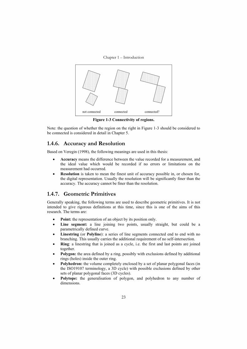
• Connectivity: is used to mean that for any two points in the region, a path can be found joining them which remains within the region. A region which has this property is known as a connected region.
Chapter 1 – Introduction
23
not connected connected connected?
Figure 1-3 Connectivity of regions.
Note: the question of whether the region on the right in Figure 1-3 should be considered to be connected is considered in detail in Chapter 5.
1.4.6. Accuracy and Resolution Based on Veregin (1998), the following meanings are used in this thesis:
• Accuracy means the difference between the value recorded for a measurement, and the ideal value which would be recorded if no errors or limitations on the measurement had occurred.
• Resolution is taken to mean the finest unit of accuracy possible in, or chosen for, the digital representation. Usually the resolution will be significantly finer than the accuracy. The accuracy cannot be finer than the resolution.
1.4.7. Geometric Primitives Generally speaking, the following terms are used to describe geometric primitives. It is not intended to give rigorous definitions at this time, since this is one of the aims of this research. The terms are:
• Point: the representation of an object by its position only. • Line segment: a line joining two points, usually straight, but could be a
parametrically defined curve. • Linestring (or Polyline): a series of line segments connected end to end with no
branching. This usually carries the additional requirement of no self-intersection. • Ring: a linestring that is joined as a cycle, i.e. the first and last points are joined
together. • Polygon: the area defined by a ring, possibly with exclusions defined by additional
rings (holes) inside the outer ring. • Polyhedron: the volume completely enclosed by a set of planar polygonal faces (in
the ISO19107 terminology, a 3D cycle) with possible exclusions defined by other sets of planar polygonal faces (3D cycles).
• Polytope: the generalisation of polygon, and polyhedron to any number of dimensions.

Chapter 1 – Introduction
24
At present, there is significant disparity in the GIS industry as to the exact definitions of these concepts, and issues such as what constitutes validity (van Oosterom et al. 2004).
1.4.8. Layers In many GIS and spatial data models, it is practice to divide the data into “layers”, frequently on the basis of thematic content (e.g. into drainage features, transport features etc.) It is also common for structural connectivity and validity constraints to be restricted to relationships between features within the same layer. For example, it may be mandated that drainage basins cannot overlap, while it is possible for them to overlap vegetation type regions without restriction. Where the individual layers have an internal structure of this type, the term “structured layer” will be used.
1.4.9. Dimensionality In this document, the descriptions are generally couched in terms of the three dimensional cases. Thus, the term half space (to be defined in Chapter 3), is used to refer generically to the half space, or the half plane (in 2D), or the half line (in 1D).
By contrast, many of the diagrams are drawn to illustrate a 2D case. This is simply due to the difficulties in representing complex 3D situations, so wherever the 2D case is sufficient to illustrate the situation being discussed, it is used.
1.5. Computational Representation of Vector Spatial Data
The Open Geospatial Consortium Abstract Specification Topic 2: Spatial Referencing by Coordinates (OGC 2002) describes the processes of determining coordinate representations of "Dimensional World" locations, and the reverse. Ultimately the locations can be represented as tuples of real numbers – e.g. (latitude, longitude), (x, y, z) etc. However the numbers themselves must be represented digitally and since a real number cannot be directly stored as a value, typically either integer or floating point representation will be used. This inevitably introduces an approximation on initial data capture, and rounding errors in individual calculations. Thus the question of countability and infinity need to be discussed.
1.5.1. Countability and Infinity A countable set is one whose members can be put into 1-1 correspondence with a subset of the set of counting numbers {1, 2, 3, …} (i.e. “counted”). All finite sets are therefore countable, but a set can be infinite and countable. Examples of finite (and therefore countable) sets include the set of all floating point numbers; the grid points within any region in a gridded representation; and the set of all possible bit patterns that can be stored in a digital computer. Infinite countable sets include the integers (including negatives), the rational numbers (Archbold 1964; Weisstein 2005) and the number of points in a region defined by points with rational number coordinates. Uncountable sets include the set of real

Chapter 1 – Introduction
25
numbers, and the set of mathematical points on a line (Courant and Robbins 1941). Note that this means that the set of points on a line is “very much larger” than the set of rational numbers.
1.5.2. Numbers The discipline of mathematics defines several classes of numbers, starting from the most basic “natural” or counting numbers. From these, the integers are defined (to allow closure of the subtraction operation) followed by the rational numbers (to allow partial closure of division), and finally the real numbers (Burkill 1964). These systems are all abstractions, and are assumed to be unbounded. That is to say, there is no largest integer, and any two unequal rational numbers will have an infinite number of further rational numbers between them. Likewise, there exists a real number whose square is exactly 2, and one with the exact value of the circumference of a circle divided by its diameter (π). The real numbers and the rational numbers form mathematical fields (meaning they satisfy the field axioms) (Patterson and Rutherford 1965; Weisstein 1999d) (see Appendix I.1).
1.5.3. Computation Numbers A computer representation has certain restrictions. Since all computers are finite objects, there is clearly no such thing as an infinite representation. Numbers are typically stored in one of two primitive forms, known as integers and floating point numbers. It is important to note that the term “integer” in a computational representation is a restricted version of the mathematical integer, in that it has a maximum and minimum allowable value. Thus it is more correctly a “domain-restricted integer”. Any programs using integer arithmetic must be aware of the possibility of numeric overflow.
Some computer languages – such as Java – define an integer representation with no restriction of size. In Java, it is called “BigInteger” (Sun 2003). This, for all practical purposes, is a true representation of a mathematical integer, and has correct computational behaviour. Although it is not truly infinite, the results of any arithmetic on any reasonable values can be expected to give the correct answer. It is not necessary to consider the possibility of overflow in BigInteger operations.
A floating point number is recorded as a characteristic, and an exponent (Goldberg 1991). Thus it is able to approximate a real number. Like the integer, it has a largest and a smallest allowable value (but these are very large in magnitude). On the other hand, they are limited in precision (there exist pairs of floating point numbers without any other between them), and do not obey the field axioms.
Java also defines a BigDecimal number representation which allows arbitrary precision in a number which is not an integer. This is not an exact representation of a real number, but an approximation with unrestricted accuracy. Thus for example, it is not possible to represent 1/3 exactly, or 2 , or π. Any division operation on a BigDecimal number has to specify at what number of decimal places rounding is to occur.

Chapter 1 – Introduction
26
1.5.4. Rational Numbers Rational numbers can be represented and manipulated within a computer fairly readily. A rational number r can be represented as an ordered pair of integers (I, J) with the interpretation r = I/J. The basic arithmetic operations can be defined in the obvious way (Courant and Robbins 1941) – e.g. if r = (I1, J1) and s = (I2, J2), then:
r+s is defined as ((I1J2 + I2J1), J1J2), r.s is defined as (I1I2, J1J2).
It is not possible in theory to implement infinite precision rational numbers, since any computer is finite in capacity. In practice, however, it is possible to define numbers using a representation such as BigInteger which has no explicit bounds, so that in any mathematical operation, sufficient resources can be devoted to the result so that the correct answer can be calculated. For example, to multiply an n bit number by an m bit number, a result can be calculated if n+m bits are available. Thus, in effect, true rational numbers can be accommodated.
If, on the other hand, the range of I and J are restricted in magnitude, (for example by using a conventional computational representation such as 4 byte integers, which would lead to the limitation that -231 ≤ I, J < 231), then the term used in this thesis is “domain-restricted rational” or “dr-rational” numbers.
1.5.5. Representation of Vector Spatial Data All computer representations of spatial data with one possible exception (the unrestricted precision rational numbers - see below) are at the fundamental level gridded. That is to say, there are only a finite number of possible values for the x, y and z coordinates of points. A significant fact about gridded representations is that, at least when the grid is of fixed size6 there is a high probability (about 60%) that a line between two random points will not pass through any intermediate points of the grid. This is because for a line between two points to have an intermediate point the difference between the x and y coordinates must have a common factor, and so cannot be relatively prime. The probability of two random large integers being relatively prime is 6/π2 (Castellanos 1988; Weisstein 2006b).
6 And probably in the case of variable sized grids as well, but this needs investigation.
Chapter 1 – Introduction
27
dx = 16
dy = 9
dx = 15
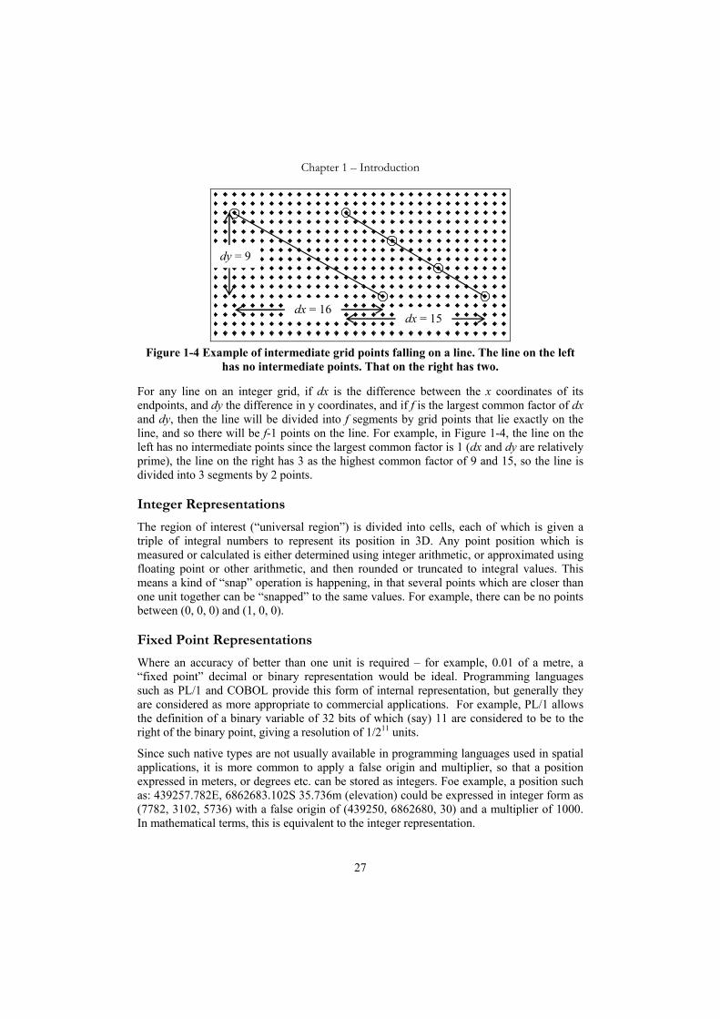
Figure 1-4 Example of intermediate grid points falling on a line. The line on the left
has no intermediate points. That on the right has two.
For any line on an integer grid, if dx is the difference between the x coordinates of its endpoints, and dy the difference in y coordinates, and if f is the largest common factor of dx and dy, then the line will be divided into f segments by grid points that lie exactly on the line, and so there will be f-1 points on the line. For example, in Figure 1-4, the line on the left has no intermediate points since the largest common factor is 1 (dx and dy are relatively prime), the line on the right has 3 as the highest common factor of 9 and 15, so the line is divided into 3 segments by 2 points.
Integer Representations
The region of interest (“universal region”) is divided into cells, each of which is given a triple of integral numbers to represent its position in 3D. Any point position which is measured or calculated is either determined using integer arithmetic, or approximated using floating point or other arithmetic, and then rounded or truncated to integral values. This means a kind of “snap” operation is happening, in that several points which are closer than one unit together can be “snapped” to the same values. For example, there can be no points between (0, 0, 0) and (1, 0, 0).
Fixed Point Representations
Where an accuracy of better than one unit is required – for example, 0.01 of a metre, a “fixed point” decimal or binary representation would be ideal. Programming languages such as PL/1 and COBOL provide this form of internal representation, but generally they are considered as more appropriate to commercial applications. For example, PL/1 allows the definition of a binary variable of 32 bits of which (say) 11 are considered to be to the right of the binary point, giving a resolution of 1/211 units.
Since such native types are not usually available in programming languages used in spatial applications, it is more common to apply a false origin and multiplier, so that a position expressed in meters, or degrees etc. can be stored as integers. Foe example, a position such as: 439257.782E, 6862683.102S 35.736m (elevation) could be expressed in integer form as (7782, 3102, 5736) with a false origin of (439250, 6862680, 30) and a multiplier of 1000. In mathematical terms, this is equivalent to the integer representation.

Chapter 1 – Introduction
28
Floating Point Representations
It is also fairly common to use floating point numbers to represent geographical coordinates. There is no need for details here, but it should be noted that in 64 bit representations there are a maximum of 264 possible numbers that can be recorded. Though large, this is finite. A false origin is often also applied in this case. As a finite representation, the issue of snapping of points still applies, and this representation is also gridded. In this case, the grid size varies over the universal region, with the spacing being finer closer to the false origin.
It should be noted that the floating point numbers are a subset of the rational numbers, where the denominators are constrained to be a power of 2. Conventional floating point numbers are also domain-restricted.
Domain-Restricted Rational Number Representation and Dual Grid
Where rational numbers are used, but where the magnitudes of the numerators and denominators are constrained to a predefined range (see Section 1.5.4) – as in the domain- restricted rational number representation to be introduced in Section 4.4, and in the dual grid approach (Lema and Güting 2002) (see Section 3.4.4), there is an underlying finite grid, albeit much finer than any of the above.
Unrestricted Precision Rational Number Representations
It is a moot point whether these are gridded or not. It is possible using an unrestricted precision integer representation (such as BigInteger) for I and J, to define a rational number r (as I/J) which thus can be as finely structured as necessary. That is to say for any two rational numbers in this form, there can be arbitrarily many rational numbers between them.
Thus it can be said that this approach is not gridded, since no matter how close two points are together, it is still possible to define representable points between them, therefore no snapping is ever needed (unless the capacity of the machine is exceeded). The use of unrestricted precision rational numbers is discussed in Section 3.4.6.
1.6. Contribution of this Work This research has shown that it is possible to rigorously define spatial primitives and operations between them in the computational domain, and in particular has led to the definition of a representation for spatial objects (called the regular polytope), which provides a solid foundation for the investigation of rigorous spatial logic. It will be shown in later chapters that it is possible to implement this representation within a database management system, associated with manipulation software to exhibit this rigorous logic. Thus it is possible to draw provable logical inferences from the spatial data stored in a digital computer.
This is shown to provide the basis for a “tool kit” of functionality where the individual functions can be applied in any combination with no possibility of incorrect results. That is to say, the sort of logic failures documented in the Case Studies of Chapter 2 cannot arise.

Chapter 1 – Introduction
29
1.7. Organisation of the Thesis The thesis is structured as follows:
Chapter 1 (this chapter) introduces the motivation for the research, and the specific problem being addressed, delineates the scope of the research, and defines some of the nomenclature to be used. Finally there is a summary, including the contribution of this research and an overview of the thesis.
Chapter 2 identifies a number of case studies which illustrate some of the major issues involved in currently used digital representations of spatial data. In most of these instances, a significant failure of the logic of the computer representation can occur, albeit in rare circumstances.
Chapter 3 presents a perspective on the history and current status of the field, and reviews some of the alternative approaches that have been, and are being investigated by other researchers. Research into the specific issue of representing the spatial information in computer form is highlighted in this chapter, rather than the larger body of work that concentrates on the mathematical model, some examples of which are included as background information.
Chapter 4 introduces a construct which has potential in addressing and solving the issues. This is named the “regular polytope”, and is rigorously defined. The properties are explored, and the space of regular polytopes is shown to be a metric topology, and to be a Boolean algebra. In addition, the regular polytope is shown to be “regular” in the topological sense (see Section 1.4.4). Finally, the issue of detection of overlap and equality is explored, first for the purely integer-based representation, and then for a representation based on rational numbers with a limited range of quotients and divisors.
Chapter 5 addresses the issue of connectivity, which is a critical issue in the storage, query and manipulation of spatial data. In seeking a useful definition, it is found that a single definition is not sufficient to all requirements, so the two most useful (to be known as Ca and Cb)7 are discussed in detail. Finally, these are applied to the regular polytope representation of spatial regions, using the integer and the domain restricted (finite precision) rational representations as defined in Chapter 4.
Chapter 6 discusses alternative approaches to spatial algebra, and relates the functionality of the regular polytope representation to these. The expressiveness of the regular polytope approach is considered in relation to: The regional connection calculus (Randell et al. 1992), The proximity space (Naimpally and Warrack 1970) and the Boolean connection algebra (Stell 1999). Use is also made of the "Egenhofer 9-intersection matrix" in these discussions for comparison purposes. This is followed by a discussion of the richness of the algebra provided in comparison with other possibilities. Finally, the relationship between this work and the constraint database (Kuper et al. 2000) approach is explored.
7 These will be defined in Chapter 5, but Cb is strong connection – where objects of dimensionality d meet at a hyper-surface of dimensionality at least d-1. Ca is weak connectivity, and only requires (at least) one point of contact.

Chapter 1 – Introduction
30
Chapter 7 presents some alternate data models that could be used to implement the approach in a database management system. For comparison purposes, a brief summary of conventional vertex representation of polyhedra is included. A basic data model for storage of spatial data in regular polytope form is then described. An alternative model, the “approximated polytope”, is introduced which, while retaining the rigour of the regular polytope will address some practical issues, using a storage form more closely aligned to the point/line/polygon paradigm. Also included are basic strategies for topological encoding, with a discussion of practical issues raised by these models.
Chapter 8 describes the implementation of a demonstration set of Java classes, intended as a tool for the practical review of the approach. The implementation is described, the test cases illustrated and some of the practical considerations that arose as a result documented. Special reference is made to the significant issue that arises in cadastral applications of the mixture of 2D and 3D definitions. This chapter gives an indication of the further development that is needed for a full implementation, and contains a discussion of the practicalities involved in converting geo-information to the regular polytope form from the conventional vertex representations.
Chapter 9 Revisits the case studies from Chapter 2 to highlight their solutions using the regular polytope.
Chapter 10 contains the conclusions that can be drawn from the research, summarising the findings in terms of the research question and the results obtained. There is scope for further research in this subject area, and this is also identified.
A bibliography of references follows.
Appendix I contains a summary of the definitions, axioms and assumptions used throughout the thesis.
Appendix II contains proofs of assertions that apply to half spaces, as made in the body of the work.
Appendix III contains proofs of assertions that apply to the integer representation of regular polytopes.
Appendix IV contains proofs of assertions that apply to the domain-restricted rational number representation of regular polytopes.
Appendix V contains the header documentation for selected classes and methods from the Java implementation discussed in Chapter 8.
Appendix VI contains the details of the encoding used in the Java demonstration classes.
Appendix VII contains some calculations of data storage requirements that can be expected for the various data models proposed in Chapter 7. Also included, for comparison are some estimated requirements for similar objects to be stored as conventional vertex representations with and without topological encoding.

Chapter 2
Case Studies
Chapter 1 has discussed the motivation and objectives of this research, defined nomenclature, introduced some number theory, and in particular highlighted the “gridded” nature of vector spatial data. In order to illustrate the issues that this raises in more detail, a number of case studies have been chosen, which have the same underlying root cause – the fact that the arithmetic calculations carried out within the computer are not exact, and do not produce the mathematically correct real number result that theory predicts. It might be thought that the result of small differences between expected results and actual calculations would be trivial, but this is not always so, as the following cases illustrate. Many of the cases illustrate the point that a Boolean valued function of spatial objects is a construct that requires caution.
The functionality provided by spatial database management systems is couched in the language of topology. For example, the words "union", "intersection" etc, are used in the form of function names in SQL statements such as:
select union(mytable.geometry, :fixed_geom) from mytable where ...;
The behaviour assigned to these functions, generally speaking, approximates to the usual topological or set theoretical meanings of these terms. This leads to the impression that these functions satisfy the axioms for union, intersection etc. as defined in the mathematical literature. This is unfortunately, not the case, as several of the following case studies indicate. It is important to note that these failures are symptoms of the lack of a rigorous underlying logic, and should not be interpreted as the problem itself. Individual solutions to each problem may well be available, but a consistent solution to all such problems is being sought.
Chapter 2 – Case Studies
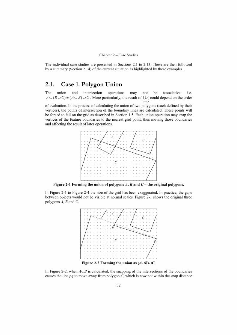
32
The individual case studies are presented in Sections 2.1 to 2.13. These are then followed by a summary (Section 2.14) of the current situation as highlighted by these examples.
2.1. Case 1. Polygon Union The union and intersection operations may not be associative. i.e.
CBACBA ∪∪≠∪∪ )()( . More particularly, the result of niiA
..1=U could depend on the order
of evaluation. In the process of calculating the union of two polygons (each defined by their vertices), the points of intersection of the boundary lines are calculated. These points will be forced to fall on the grid as described in Section 1.5. Each union operation may snap the vertices of the feature boundaries to the nearest grid point, thus moving those boundaries and affecting the result of later operations.
A C
B
Figure 2-1 Forming the union of polygons A, B and C – the original polygons.
In Figure 2-1 to Figure 2-4 the size of the grid has been exaggerated. In practice, the gaps between objects would not be visible at normal scales. Figure 2-1 shows the original three polygons A, B and C.
A C
B
p
q
Figure 2-2 Forming the union as (A∪B)∪C.
In Figure 2-2, when A∪B is calculated, the snapping of the intersections of the boundaries causes the line pq to move away from polygon C, which is now not within the snap distance

Chapter 2 – Case Studies
33
(one unit of the grid). As a result, (A∪B)∪C evaluates to two regions which are not connected.
A C
B
Figure 2-3 Forming the union B∪C first.
With the operations applied in the other order as depicted in Figure 2-3, C would have been within the snapping distance of B as B∪C was formed. Thus the result of the calculation of A∪(B∪C) is a single contiguous region as seen in Figure 2-4.
A C
B
Figure 2-4 The Result of A∪(B∪C).
In this case, there is a qualitative difference in the result, depending on the order of calculation. This is a rare case in practice, but there is frequently a numerical difference in the calculated result depending on order of calculation. This kind of event effectively prevents the "design by contract" approach discussed in Section 1.4.2. For example – the receiving party may require that all the regions are contiguous – determined by calculating A∪B∪C. The data supplier validates the data by calculating A∪(B∪C), and transmits the features – assuming they are correct. The receiving party calculates (A∪B)∪C and rejects the regions as non-contiguous.

Chapter 2 – Case Studies
34
2.2. Case 2. Data Interchange Using interchange protocols such as GML (Geography Markup Language)(OGC 2000), and the more recent GML3 (ISO-TC211 2004) the transfer of coordinate values is in decimal numbers with finite precision. This means that the consistency of the data can and does change as a result of the transmission. Thus a feature which is valid before transmission may be invalid after transmission. The basic problem is that a Boolean result such as a test for validity depends on the results of calculation using finite arithmetic, so that even a small calculation or rounding error may lead to a qualitatively different result.
A possible solution is to apply a tolerance, so that for a feature to be valid1 it must not have any points within a distance of ε of any other point or line. This is the approach suggested by Milenkovic (1988), and will be discussed further in Chapter 3.
d
invalid polygon may be invalid at tolerance > d
Figure 2-5 Self-intersection in a polygon.
The polygon on the left in Figure 2-5 is considered invalid, the one on the right is valid, but if the points are moved small distances, it may become invalid. If d < ε, the polygon on the right would not be considered to be valid at tolerance ε. It could be argued that the receiving software could automatically correct the error if d < ε, but this raises further issues. Prior to transmission, the polygon on the right is a single connected polygon. If the error is corrected, it becomes a pair of polygons in contact. This would not be valid if the contract was for a single polygon.
It might be thought that applying such a tolerance ε, where ε is significantly larger than any potential loss of resolution would solve the problem of transmission in some protocol like GML. For example, if all features are valid at tolerance ε, and they are transferred with sufficient number of decimal digits that the inaccuracy introduced (say r) is less than ε, the features will be valid on arrival. This is not a solution per se, since on arrival the features can no longer be asserted to be "valid at tolerance ε". While they will be guaranteed to be valid at tolerance ε-r, any attempt to standardise the definition of "valid" in terms of a
1 In the Milenkovic Normalisation, this is a validity requirement. It will be suggested later that this be re-interpreted as a “robustness” parameter – see Section 2.4.
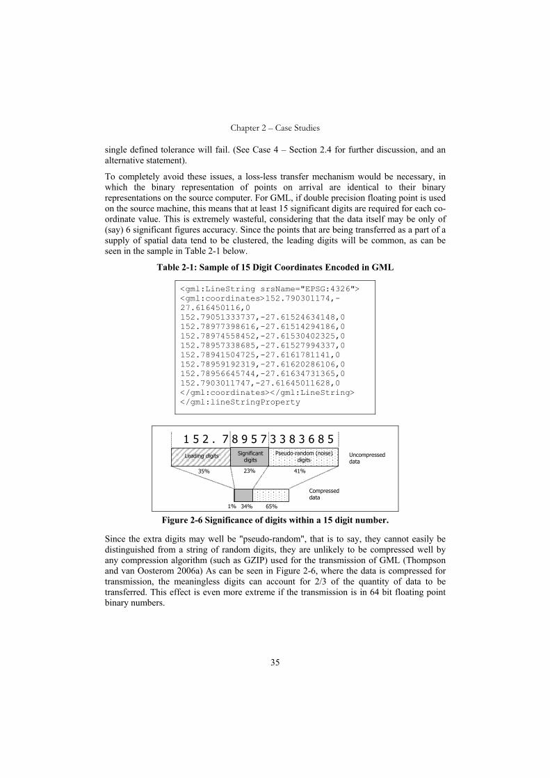
Chapter 2 – Case Studies
35
single defined tolerance will fail. (See Case 4 – Section 2.4 for further discussion, and an alternative statement).
To completely avoid these issues, a loss-less transfer mechanism would be necessary, in which the binary representation of points on arrival are identical to their binary representations on the source computer. For GML, if double precision floating point is used on the source machine, this means that at least 15 significant digits are required for each co-ordinate value. This is extremely wasteful, considering that the data itself may be only of (say) 6 significant figures accuracy. Since the points that are being transferred as a part of a supply of spatial data tend to be clustered, the leading digits will be common, as can be seen in the sample in Table 2-1 below.
Table 2-1: Sample of 15 Digit Coordinates Encoded in GML
<gml:LineString srsName="EPSG:4326"> <gml:coordinates>152.790301174,-27.616450116,0 152.79051333737,-27.61524634148,0 152.78977398616,-27.61514294186,0 152.78974558452,-27.61530402325,0 152.78957338685,-27.61527994337,0 152.78941504725,-27.6161781141,0 152.78959192319,-27.61620286106,0 152.78956645744,-27.61634731365,0 152.7903011747,-27.61645011628,0 </gml:coordinates></gml:LineString> </gml:lineStringProperty
Leading digits Significant digits
Pseudo-random (noise) digits
35% 23% 41%
1% 34% 65%
Uncompressed data
Compressed data
1 5 2 . 7 8 9 5 7 3 3 8 3 6 8 5
Figure 2-6 Significance of digits within a 15 digit number.
Since the extra digits may well be "pseudo-random", that is to say, they cannot easily be distinguished from a string of random digits, they are unlikely to be compressed well by any compression algorithm (such as GZIP) used for the transmission of GML (Thompson and van Oosterom 2006a) As can be seen in Figure 2-6, where the data is compressed for transmission, the meaningless digits can account for 2/3 of the quantity of data to be transferred. This effect is even more extreme if the transmission is in 64 bit floating point binary numbers.

Chapter 2 – Case Studies
36
2.3. Case 3. ISO 19107 Definition of Equality Since the equivalence relation axioms are referred to here and later, and are pertinent to the definition of equals()2 in ISO 19107 (ISO-TC211 2001), they are restated here:
R is an equivalence relation on set X if it is:
Reflexive: aRa ∀a∈X Symmetric: aRb ⇒ bRa ∀a, b∈X Transitive: aRb, bRc ⇒ aRc ∀a, b, c ∈ X. (Weisstein 1999c)
One interpretation of the “equal” relational operator a = b between spatial representations would be truth of the proposition “a is an equivalent representation of the same (or identical) real-world feature as represented by b, and is of the same accuracy”.
The ISO 19107 definition of equals() (ISO-TC211 2001) uses the phrase "shall return true if this GM_Object is equal to another GM_Object", but qualifies this definition with: "Since an infinite set of direct positions cannot be tested, the internal implementation of equal must test for equivalence between two, possibly quite different, representations. This test may be limited to the resolution of the coordinate system or the accuracy of the data. Application schemas may define a tolerance that returns true if the two GM_Objects have the same dimension and each direct position in this GM_Object is within a tolerance distance of a direct position in the passed GM_Object and vice versa" (ISO 19107 Section 6.2.2.18.3).
This definition has several weaknesses:
• The implementation is problematic since the number of possible representations which are (set-theoretically) equal to a given polygon, while not actually infinite, is very large. In many cases the operation will be implemented by making the assumption that two objects are equal if and only if their representations are defined by the same number of points in approximately the same positions. If this implementation is used, a redundant point such as that introduced in parcel E in Figure 2-8 is significant, but should not be, according to the ISO 19107 definition.
• It is not definitive – the choice of a tolerance value and the technique for applying that tolerance are left to the application schema. Thus a pair of objects may be equal in one implementation, but cease to be equal in another.
• It is not transitive – it is quite likely, using this definition that a.equals(b), and b.equals(c), but not a.equals(c) For an example using point features, see Figure 2-7. (Note that the “ideal” definition given above is transitive).
2 This syntax, of following a function name by a pair of parentheses, is taken from several programming languages, and is used in the ISO 19107 standard.

Chapter 2 – Case Studies
37
a
b
c
Figure 2-7 Three points (with tolerance shown) illustrating breakdown of equality.
In order to further explore this issue, Figure 2-8 has feature A being compared with the other features B to F. It is assumed that circled vertices are identical to the corresponding vertices in A, but those circled in dotted line (e.g. vertex 3 of D) are only approximately equal (differing by a small rounding error). It is further assumed that the direction of encoding is standardised (and must be anticlockwise).
4
3
2 1
4 3
2 1
2 1
4 3
4 3
2 1
4 3
2 1
5
4 3
2 1
5
A F E D C B
Figure 2-8 Simple polygon equality.
A.equals(A) should be true by identity. A.equals(B) should be true – B has the identical representation to A. A.equals(C) Here the regions are equal as point sets, but the cyclic definition of the boundary rings have different starting points. By the ISO definition they should be equal. A.equals(D) Here the regions are not exactly equal as points sets, since point 2 has been displaced by rounding. By the ISO definition they could be equal depending on a decision by the implementer, and the tolerance chosen. A.equals(E) Here the regions are exactly equal as point sets (it is assumed that point 5 is exactly on the line 1-4, and no rounding errors have been introduced). By the ISO definition they are equal. A.equals(F) This is similar to E, but (as is more likely) a small rounding error has been introduced in the calculation of point 5, and it does not lie exactly on line 1-4. Here the regions are not exactly equal as point sets. By the ISO definition they could be equal depending on a decision by the implementer.
There is no provision in the ISO definition of equals to distinguish regions other than by the transfinite set of points that are within the regions. Thus the introduction of a redundant

Chapter 2 – Case Studies
38
point (as in E), or the relabelling of points (as in C) should never be significant. The intention of the ISO definition is that all of A to F should test equal to A.
2.4. Case 4. ISO 19107 Definition of Simplicity In the ISO 19107 standard, the operation isSimple() returns true if there is "no interior point of self-intersection or self tangency" (multi part objects are allowed but should not overlap). Note that in contrast to the definition of "equals()" there is no provision for any tolerance in the definition. As a result, the ISO 19107 standard perpetuates the problems described in Case 2 Section 2.2.
s im p le g e o m e t r i e s n o n -s im p le g e o m e t r i e s
a
b
c
d
e
f
g
h
Figure 2-9 Simple and non-simple geometries.
Also in contrast to the definition of "equals()", there is no guidance given in the standard towards the implementation of an algorithm for testing "self intersection or self tangency". This is particularly serious, since many implementations treat the isSimple() requirement (or something similar) as necessary for the acceptance of a geometry. For example, polygon features cannot be entered into an Informix database (using the spatial datablade) if they have a non-simple boundary (see Figure 2-9) (IBM 2002). Note that in the cases of objects f and h in the diagram, the overlaps can be invisibly small, and still prevent acceptance. This causes problems in the creation of a corporate spatial database, and the error "polygon is self-intersecting" is a common one to be seen in the load process. In practice, it can be very difficult to locate such an error in a complicated or large feature. The “Design by Contract” approach is not possible unless the exact definition of isSimple() can be given such that all implementations can be guaranteed to produce the same answer.
It has been suggested (Thompson and van Oosterom 2006a) that, rather than defining a Boolean operation ("isValid()" or "isSimple()" etc.), the tolerance as discussed in Case 2 be replaced by a "robustness" parameter ρ, defined such that the movement of all points by a distance of < ρ in different directions will be guaranteed to leave the object in a "simple" state. A large robustness value would indicate a "robust" representation, while a small value

Chapter 2 – Case Studies
39
should be a warning of potential problems. In the context of "Design by Contract", if a module is intending to undertake some action which may introduce a relative perturbation of the points of a region, it should contract for a region with a sufficiently large robustness value.
For example, if a polygon is robust at 10cm, and it is to be transferred in a form that introduces errors of up to 1 cm, it can be contracted to arrive valid and simple, but can only be asserted now to have a robustness of 9cm, and can immediately be used in any application for which a robustness of 9cm is sufficient. It could not have been contracted to be delivered using a transport mechanism that could introduce relative errors greater than 10cm. Note that on arrival, the robustness parameter could be re-calculated and might be found to be better than 9cm. In fact, it could have even improved to 11cm, but the important issue is that the data can be used without revalidation.
2.5. Case 5. Intersection of a Point with a Line In ISO 19107, the function line.contains(point) is intended to determine whether a point lies within the line. (This function is one of the specialisations of GM_Object.contains(point)3. Another specialisation of this parent is the more useful function polygon.contains(point).)
A function like this is extremely problematic, being sensitive to rounding conditions in its computation. This sort of function is usually present for “completeness” – so that, for example, a point is either within a polygon, outside the polygon, or on its boundary (thus on the line). In 2D, the relationship between point (x, y) and line (x1, y1) to (x2, y2) might be determined by evaluating ))(())(( 112121 xxyyxxyy −−−−− , and interpreting a negative result as “left of line”, greater than zero as “right of line” and zero as “on the line”.
In general, the set of points that would test as “on the line” is sparse in computational space. As was noted in Section 1.5.5, in an integer based representation approximately 60% of all straight lines will not pass through any grid points apart from the endpoints. The calculation of the intersection of two lines will in general produce a point which has been approximated to the nearest representable values (as integer or floating point). It is unlikely that this point will test as contained by either line.
Practical GIS implementations “get around” these problems either by breaking lines to force them to pass through the point (as described in Case 9, Section 2.9), or complex and difficult special case handling, but still problems arise. One example might be that the use of a tolerance to determine a point's containment in a line can lead to a situation where a point is simultaneously "on" two non-parallel lines while being a considerable distance from the point of intersection of those lines. Without a tolerance, the intersection of two lines may not be on the lines, with a tolerance, a point can be on both lines but not be the intersection. These problems can manifest themselves as “bugs”, but are more correctly symptoms of failure of the underlying logic.
3 GM_Object is the super class for all geometric objects. I.e. all other geometric objects are subclasses of it.

Chapter 2 – Case Studies
40
Figure 2-10 Example of a point "on" two lines, but
not at their intersection.
The intersection of the lines in Figure 2-10 would probably be calculated as the point marked , but the circled point would be tested as on both lines. See Section 3.2.12 for a discussion of these tolerances in terms of the co-Heyting algebra formulation of Worboys (1998).
2.6. Case 6. Narrow Cadastral Parcels
A
B
C
E
p q
Figure 2-11 Narrow cadastral parcel and adjoiners.
In Figure 2-11, parcel E (presumably the result of negotiations following an encroachment) is 100mm wide at the top. Note that the lower vertex p is about 100 mm south of the common boundary between B and C (point q), and that point q is about 0.3 mm east of the common line between A and E.
This is acceptable to most current systems, but when converted from one datum to another, all co-ordinate values are rounded to the nearest integer – of the order of millimetres at ground scale. It would normally be thought that 1 mm at ground scale would be accurate enough, and in fact it is much finer than the true accuracy of the data, but the result is as shown in Figure 2-12 (with the effect exaggerated).
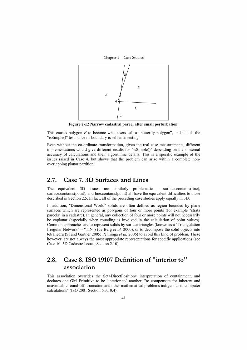
Chapter 2 – Case Studies
41
A
B
C
E
p
q
Figure 2-12 Narrow cadastral parcel after small perturbation.
This causes polygon E to become what users call a “butterfly polygon”, and it fails the "isSimple()" test, since its boundary is self-intersecting.
Even without the co-ordinate transformation, given the real case measurements, different implementations would give different results for "isSimple()" depending on their internal accuracy of calculations and their algorithmic details. This is a specific example of the issues raised in Case 4, but shows that the problem can arise within a complete non-overlapping planar partition.
2.7. Case 7. 3D Surfaces and Lines The equivalent 3D issues are similarly problematic - surface.contains(line), surface.contains(point), and line.contains(point) all have the equivalent difficulties to those described in Section 2.5. In fact, all of the preceding case studies apply equally in 3D.
In addition, "Dimensional World" solids are often defined as region bounded by plane surfaces which are represented as polygons of four or more points (for example "strata parcels" in a cadastre). In general, any collection of four or more points will not necessarily be coplanar (especially when rounding is involved in the calculation of point values). Common approaches are to represent solids by surface triangles (known as a "Triangulation Irregular Network" – "TIN") (de Berg et al. 2000), or to decompose the solid objects into tetrahedra (Si and Gärtner 2005; Penninga et al. 2006) to avoid this kind of problem. These however, are not always the most appropriate representations for specific applications (see Case 10. 3D Cadastre Issues, Section 2.10).
2.8. Case 8. ISO 19107 Definition of "interior to" association
This association overrides the Set<DirectPosition> interpretation of containment, and declares one GM_Primitive to be "interior to" another, "to compensate for inherent and unavoidable round-off, truncation and other mathematical problems indigenous to computer calculations" (ISO 2001 Section 6.3.10.4).

Chapter 2 – Case Studies
42
That is to say, since the test of GM_Object::contains() may give an incorrect result, (for example, as explained earlier in Section 2.5), the fact of containment must be stored as an association.
The approach is problematic, since it is only required if the contains() does return a wrong answer, thus is implementation specific. One particular implementation may correctly detect containment, and therefore not deem it necessary to explicitly record the "interior to" association. Another implementation which is processing this data may not detect the containment using the contains() operation, and infer from the lack of the explicit association that containment is counter-indicated.
Any attempt to encode all “interior to” associations for all objects in a database is quite problematic, since for any point in the universe of discourse, there can be a vast number of regions that it is interior to – for example, state, suburb, town, country, economic region, climatic zone, etc.
2.9. Case 9. Adjoining polygon points In cadastral databases, a common technique to handle the subdivision of an adjacent lot is the insertion of an additional point (a node in topologically structured data):
A
B
C
p
a
b
Figure 2-13 Subdivision of adjoining parcel.
In Figure 2-13, after the subdivision of the parcel adjoining A to create parcels B and C, Point p is also made a part of the definition of parcel A, which thereby becomes a five-sided polygon. This is necessary because the representation of the point p as calculated is unlikely to fall exactly on line ab (i.e. ab.contains(p) does not necessarily return true), and has several unfortunate effects:
1. The original line ab, no longer exists in the database, and so any attributes (e.g. measured bearing and distance) that attached to it must be managed in some other way.
2. If a locking strategy is in use, it is necessary to lock parcel A, even though it is not really being changed in any way. This can cause escalation of locks, and make deadlock more likely. It also creates an update to parcel A.
3. As discussed earlier, by the ISO 19107 definition of equals() (ISO-TC211 2001), if A is the original 4 sided parcel, and A' is the parcel after the update, with point p included in

Chapter 2 – Case Studies
43
its perimeter, A.equals(A'), since every direct position within A is within an acceptable tolerance of some point in A', and vice versa. Thus a parcel has been replaced by an equal parcel. This highlights one of the difficulties which can be caused by confusing equality of the digital representation with equality of the mathematical abstraction. (See also Case 13, Section 2.13 for programming difficulties this may cause).
2.10. Case 10. 3D Cadastre Issues An equivalent problem to Case 9, of adjoining points in neighbouring objects also arises in a 3D cadastre, which is however, more complex and difficult to picture. Frequently the solutions chosen to address these problems differ significantly from those conventionally used in 2D cadastre. In practice, where volumetric parcels4 are present, they only constitute a small percentage of all property parcels. To represent all parcels in a cadastre as 3D objects is impractical at present (and probably not particularly useful).
Given current technology, hybrid approaches are most appropriate at present, where the vast majority of parcels are represented as 2D polygons, with the volumetric lots being represented as regions of space bounded by 3D flat polygons (Stoter and Salzmann 2003). Of those parcels which are volumetric, the vast majority are defined as prisms, with the sides being vertical planes, and the tops and bottoms being horizontal planes. There exists, however, a small but significant set of parcels which do not fit this classification.
As discussed earlier, a polygon of 4 or more vertices will not in general be planar, and a triangulated network is usually resorted to when modelling solid objects to prevent conflicts. This is not necessarily the best approach in the case of cadastral parcels. The practicality is that the surfaces of the parcels in "Dimensional World" are most usually intended to be flat surfaces, and the lack of planarity in the representation is a result of measurement errors and/or rounding effects. To break up what should be plane surfaces into a triangulation on the basis of measurement or rounding effects would not be productive, and would obscure the true situation.
Where volumetric parcels adjoin normal 2D parcels, a situation analogous to the above (Figure 2-13), occurs.
Figure 2-14 represents a vertical slice (side view) of a section of the cadastre. The majority of volumetric parcels are of this form. Parcels 1 and 3 are normal 2D parcels, parcel 2 has been subdivided into strata parcels 2a, 2b, 2c and 2d, by defining vertical planes (p-q), (r-s) and (t-u). Note that parcels 1, 2d and 3 have no defined top, and 1, 2a and 3 have no defined bottom.
By analogy with Figure 2-13, is it necessary to convert parcels 1 and 3 to 3D representations, so that the lines p, q, r, s, t and u are included in their definition? (In order that the surface (p-r) be a common boundary between parcel 1 and parcel 2c).
4 Normal cadastral parcels typically are defined by 2D polygons, and are taken to be unrestricted in elevation (height or depth). Volumetric parcels are defined as regions of space, bounded by (usually plane) surfaces.

Chapter 2 – Case Studies
44
z
x
1 3
2 a
2 b
2 d p q
t u
2 c r s
Figure 2-14 Volumetric parcels adjoined by normal (2D) parcels, viewed from the
side.
2.11. Case 11. Datum Conversion During the lifetime of the Digital Cadastral Data Base (DCDB) at the Department of Natural Resources & Water in Queensland, it has been necessary on two occasions to convert to a new datum (ICSM 2002). This can be expected to occur again in the future. The necessity can arise for one or more reasons: the improvement of measurement technologies can make a redefinition of datum desirable; continental drift causes a movement of local features relative to distant features; and/or policy decisions could mandate a change.
In the process of a datum change, the coordinate values of all points must be re-calculated, and this calculation is necessarily of a certain accuracy. In a database of finite precision, the result is then rounded to the accuracy of the database storage. This introduces a pseudo-random relative movement of points, since the rounding direction may vary from point to point. A further effect is that lines that were straight may become bent. This may require the insertion of intermediate points in very long lines. (Bent lines may also be straightened in some cases, as existing inaccuracies are corrected). It may also be necessary to introduce points in long (previously straight) lines where this relative movement would otherwise give rise to topology failures caused by the line crossing over, or closely approaching an unrelated point.
Any digital representation of spatial features must be sufficiently robust to allow this sort of operation without the problems of Cases 2, 3, 4 and 6 arising.

Chapter 2 – Case Studies
45
2.12. Case 12. Uniqueness of Representation
Represented as a polygon with a hole
Represented as a polygon with a continuous (one piece) outer boundary
Figure 2-15 Equal polygons (by ISO definition) with very different definition.
Where a tolerance is allowed for the test for equality, some counter-intuitive results can apply. For example, the two regions as illustrated in Figure 2-15 may be equal to within a defined tolerance, but a small miss in the points where the boundary and the internal "hole" are in close proximity may lead to a completely different representation. Thus it is possible for a region with a single simple boundary to be equal to a region with an inner hole, highlighting a difficulty likely to arise in the implementation of the ISO definition of equals.
2.13. Case 13. GeoTools/GeoAPI definition of Object.equals()
The GeoAPI and GeoTools projects (Codehaus 2006; OGC 2006) aim to develop a set of Java classes based on the OGC specifications. In the documentation of these classes, is a definition of the TransfiniteSet "equals" function, which contains a copy of the OGC (and ISO) definition. Since geometric primitive classes are required to implement the TransfiniteSet interface, they would be expected to use this definition.
On the other hand, the geometric primitives are also expected to be classes that inherit from the Object class, and so implement "equals" and "hashCode" methods. A hash code is used by various collection structures where large numbers of objects are to be dealt with. The procedure is that the hashCode method generates a key value that is meaningless except that two equal objects must generate the same hash code value. Thus it is possible to use the value as a key to provide very fast access to the object in the collection. The requirements of the hashCode method are that for two objects a and b:
a.equals(b) ⇒ a.hashCode() = b.hashCode()
¬ a.equals(b) “nearly always implies” a.hashCode() ≠ b.hashCode()

Chapter 2 – Case Studies
46
The “nearly always implies” determines how useful the hash code calculation algorithm is. If many unequal objects generate the same hash code, the algorithm is inefficient, and it is difficult to imagine any useable routine if the equals test allows a tolerance. For example, polygons D, E and F of Case 3 (see Figure 2-8), which fulfil the transfinite set definition of equality are difficult to reconcile with any hash code calculation routine based on the definition of their vertices.
2.14. Conclusions Much research has been done on the modelling of conceptual world features as mathematical constructs. The International Standard ISO 19107 can be seen as a distillation of the techniques so far developed. However, very little work has been done on the question of the final digital representation. As a result, the effects of the finite accuracy and granularity of the number representation have been left to individual programmers to solve. The ISO standard is silent on these issues, which it characterises as "implementation issues", leading to a situation where data which is ISO compliant can be transmitted to a system, also ISO compliant, which rejects that data due to different interpretations of "tolerance" as allowed by the standard. The same is true of the OGC specifications based on the ISO standards. The current situation is that of a well understood mathematical model being approximated by a digital representation which is poorly understood.
The result of this is that all data to be accepted by a client must be validated by that client. Even worse, it will have a significant likelihood of failing that validation and there is little that the data supplier can do to prevent this apart from either:
• Validating the data for use by all known software, using that software (which probably requires the purchase of a license to use that software), or
• Defining a private standard or profile, and outputting to that standard – requiring a specially tailored data load program to be written by/for the client.
While the technique of topological encoding can provide a rigorous internal logic for dealing with 2D data, the issue of transporting those data between vendors is not solved, and the situation in 3D is far from satisfactory. Where topological encoding is not used in a spatial database, or where the data are separately sourced, the operations between primitives cannot be consistently and rigorously defined.
One result of this lack of a regime of rigorous definition can be seen in the inconsistencies in meaning and behaviour of 2D polygons highlighted by van Oosterom et al. (2004). It is essential that such problems be avoided in 3D spatial databases, where the potential for confusion is so much higher.
Several specific cases have been described in this chapter, which illustrate the potential results of breakdown of the underlying logic of current practices. The next chapter will discuss various alternate approaches that have been used, or are being investigated in the search for a consistent and logical approach to spatial data storage and manipulation.
Chapter 3
Related Work and Theory
The previous chapters have introduced the class of issues that this work is addressing. The scope of the research has been defined in Chapter 1 and a series of representative “case studies” documented as practical examples of the effects of the problem being addressed in Chapter 2. These cases indicate that much work is needed on the issue of implementing spatial primitives and the operations between them within finite digital equipment.
This chapter focuses on research that has been carried out in this and related fields, and which is relevant to the work in progress. Section 3.1 gives a brief historic perspective on the broader field of representation of spatial information. Section 3.2 reviews the literature of spatial logic within a mathematical model, with an emphasis on that work that has application in the representation of spatial data in digital form. There is a significant body of work in this area, so a very brief overview approach is taken. Section 3.3 discusses literature pertinent to the numerical accuracy used in calculations and representation.
Section 3.4 covers the research that has been carried out to date directly relevant to the question of carrying the rigorous logic into the computer representation of the data itself, and on the issue of drawing inferences from a finite precision digital model. This is a significantly smaller body of work, and is accordingly covered in greater detail. Section 3.5 concludes the discussion.
3.1. Historic Perspective The history of storage, maintenance and analysis of spatial data in a digital computer representation can be summarised as a progressive increase in the amount of knowledge

Chapter 3 – Related Work and Theory
48
and attribution that is associated with the basic mapping data, and a move from personal data on a local “desktop” to the recognition of the spatial information as a corporate resource, initially as a data base, and more recently as a Geographic Information Infrastructure (GII), with the potential for sharing data between organisations.
3.1.1. Early Representations of Spatial Information The largest body of literature relating to this subject is in the domain of representing "Conceptual World" spatial phenomena as mathematical abstractions. The earliest references are lost in antiquity; in fact, one of the major drivers for the development of mathematics itself appears to have been the delineation of property boundaries. “If the river carried away any portion of a man’s lot, … the king sent persons to examine, and determine by measurement the exact extent of the loss … From this practice, I think, geometry first came to be known in Egypt, whence it passed to Greece” Herodotus – quoted by Boyer (1985 page 9). The earliest known example of what is, in effect, a cadastral “map” was found in the excavation of Catalhoyuk in central Turkey, and dated at about 6200 BCE, long before writing was developed (Brock 2001).
3.1.2. Early Digital Representation The earliest attempts to represent geographic data in computer form were limited to storing the linework and text of maps (ECU 1970). This kind of approach is characterised by standards such as AS2482 (SAA 1984), where the linework of the map is represented, with attributes limited to the type of feature represented1. Any names of features are included as "annotation", which specifies where and how the text is to be displayed, but with no meaning attached, and no semantic connection between text and linework. This approach is severely limited, especially in its ability to draw inferences from the data.
3.1.3. Feature Encoding A major improvement came with the introduction of feature encoding. This makes the critical connection between the "Dimensional World" feature, and its geographic and other stored (attribute) details. Again, this can be characterised by various standards that have been written to define interchange of feature information. An example of this type of exchange format (which became a de-facto standard) is the Shape file format (ESRI 1998), where the spatial (geometric) information of the features is located in one file, with the attribute data pertaining to those features stored in an associated dBase format2 file. This is typical of early implementations, which used a database (often relational) to store the non-geographic information, linked to a spatial data repository.
1 This attribute information is sufficient to determine how the linework should be presented on a printed or viewed map. This is, however preferable to the interchange of pure presentation information such as line weights, colour, shading etc. without any connection to the thematic and type attributes of the feature.
2 In the ESRI Shape file white paper (page 25), dBase is described as “a standard DBF file used by many table-based applications in Windows™ and DOS.” and the format is defined.

Chapter 3 – Related Work and Theory
49
3.1.4. Topological Encoding One of the biggest advances came with the introduction of "topological encoding". This has several variants, but in general records the spatial component in a way which builds connectivity between features into the data structure (Burrough and McDonnell 1998), and avoids redundancy in spatial representations. There are two forms of topological encoding in general use currently:
• Linear networks – where the features are 1D lines joining nodes. This form is frequently used for road, rail, utility, watercourse etc. modelling, and has application in route planning, electricity supply management etc.
• Space partitioning (usually in 2D, but also recently extending to 3D), where the region of interest is divided into non-overlapping sub-regions which form a complete coverage.
The spatial partitioning form is of more interest in the current context, and it provides two major advantages over discrete polygon storage of coverages:
• It gives the option of fast neighbour searches (e.g. find adjacent polygons).
• It reduces the storage requirements for boundary details.
There are several variants on topological encoding for space partitioning, but all are based on the common storage of boundary details, with links between the storage location of the boundary, and the details of the region(s) delimited by that boundary. It is in the definition of a partition3 that this approach is most significant, where every boundary is used in the definition of at least two regions (apart from those few boundaries that surround the entire coverage) (Molenaar 1998; Louwsma 2003).
A
B
1
2
left face
right face
start node
end node
Figure 3-1 Two regions delimited by a common boundary line.
In Figure 3-1, the line string between node 1 and node 2 defines region A to its left and region B to its right. It is in cases such as this, where there is some complexity in the
3 In this context, “partition” (or “coverage”) is used to mean that the entire area of interest is divided into non-overlapping regions (with no gaps between regions).

Chapter 3 – Related Work and Theory
50
definition of the common boundary, that the greatest advantages of the approach are realised. (Since the definition of the line string from 1 to 2 contains many points, which do not need to be stored twice as would be the case if A and B were defined as discrete, independent polygons).
The difficulties with topological encoding come from the representation of "Dimensional World" measurements as digital values, firstly, in the accuracy, and secondly in the quantisation of digital representation of numbers. The accuracy question of topological storage has been well researched. e.g. Hunter (1998). The quantisation issue is the subject of this research.
With the move to feature encoding, came the opportunity to derive knowledge from the stored data, and this is the major advantage of the "GIS" (Geographic Information System). The ability to determine relationships between features (e.g. overlap, nearness etc.) provided an additional benefit that helped justify the cost of digital geographic data capture.
The greatest strengths of the topological approach arise from the fact that it provides some degree of logical rigour. It is fairly simple to prove that, for example, a properly constructed collection of polygons can form a continuous, non overlapping partition of a plane, and that the operations of union, intersection etc. between polygons from within the partition have the correct behaviour.
The difficulty of logic operations on data from different sources is discussed by Burrough and McDonnell (1998 page 178). For example: "Polygon overlay can lead to a large number of spurious small polygons that have no real meaning and must be removed". All major GIS vendors provide such "cleaning" mechanisms, but the choice of parameters to eliminate spurious overlaps without destroying real information is not trivial, and in fact is a highly skilled and specialised operation. Note – in discussing "Errors and Quality Control", Burrough and McDonnell include rounding errors in the digital arithmetic with the other (measurement based) errors. This approach is far from ideal, since the characteristics of the different forms of errors are quite different4.
An investigation into the relationship between lines (Clementini and Di Felice 1998) shows the intersection of two linear features can take on a host of complex forms. For example, where curved lines are allowed, lines could intersect at a number of points, and some intersections may be tangential, in the form of a cusp, etc. However, this does not address the digital representation. The interactions of area and volume features exhibit even more complexity.
A fundamental issue with drawing inferences from geographic data is assessing the "fitness for use" of that data (Goodchild 1998). In particular, questions such as connectivity of regions can give completely wrong answers if posed loosely using incompatible data5.
4 For example, measurement based errors are generally of a larger magnitude than rounding errors, and usually manifest one time only – at the time of data capture. The rounding errors potentially accumulate at every instance of data manipulation. 5 For example, if the polygon overlay "cleaning" mechanism as described above is not wholly successful, spurious overlaps can be reported, and connection/adjacency may be missed.

Chapter 3 – Related Work and Theory
51
Agumya and Hunter (1999) propose a "risk based" approach to the problem. This has merit, but does require a clear understanding of risk management issues by the user.
Jeansoulin discusses the use of explicit spatial constraints in conjunction with computed topologic relationships, observing that "The point location tolerance is one of the most investigated sources of geographic error. But its consequences on several other geographic aspects (topology, network connectivity, etc.) are not easy to automate …" (Jeansoulin 1998 page 108). An interesting concept in this paper is the use of the term "pre-compiled information" to refer to the topological relationships contained in the storage structure of topologically encoded data. This is a useful concept, since it highlights the decision making processes which are part of the topology cleaning activity, and which may not be recognised as such by the user.
In particular, where a database of spatial information is constructed using topological encoding, the division of the database into "structured layers" is a critical decision, since the topological relationships are normally only compiled within a single layer. Any cross-layer relationships are usually to be constructed "on the fly", and are thus subject to the failures of rigour associated with non-topologically encoded data.
The process of compiling topological relationships between regions within the same layer (the so-called topology generation or cleaning operation) requires a high level of skill and understanding of the problem by the human operator if the correct relationships are to be generated.
3.1.5. 3D Topology The use of topological encoding within a database can, as described, provide a limited form of rigorous logic (restricted to single layer, single vendor, and only where pre-compiled and explicitly stored), but to the present time, this has been commercially implemented in the 2D case only.
Current research on the inclusion of 3D objects in a spatial database includes the work of Arens, Stoter and van Oosterom (2003). This is a practical approach to the problem, based on the requirements of cadastre, telecommunications and town planning, but the topological encoding is restricted to being internal to individual objects. Topology between the objects is not maintained, although the paper does not close the door on future work in this direction. The Oracle corporation has developed a data model based on the GML3 specification which does include 3D topological encoding (Kazar et al. 2007).
The “Tetrahedronized Irregular Network” (TEN) is an extension of the “Triangulated Irregular Network” (Peucker et al. 1978) into three or more dimensions. Although 3D is the most useful in practical problems, the theory is fully general, and makes no assumption of restricted dimensionality. The TIN has proved very useful in the representation of a scalar (or vector) function of two variables - including, but not restricted to geographic coordinates (Tse and Gold 2002). For example, the TIN is frequently used for the representation of the elevation of a land surface, on the assumption that there are no overhanging or vertical cliffs. The TEN structure decomposes solid objects or regions into tetrahedral units (in nD, generalised to simplexes) (Penninga et al. 2006), with each surface (hyperplane) encoding the tetrahedron (simplex) on each side of it. This provides a topological encoding of adjacency.

Chapter 3 – Related Work and Theory
52
Research is proceeding on the practical problems of a 3D cadastre (Stoter and Salzmann 2003; Stoter and van Oosterom 2006), where the inclusion of a relatively small number of volumetric objects in what is primarily a 2D polygon coverage is addressed. This research highlights the advantages of a topological representation of the 2D objects, but recognises the impracticality of a full 3D database. Instead a hybrid approach is recommended. The decision as to whether the 3D components should be topologically encoded is addressed in these works, but is still the subject of further investigation.
What has been recognised is that "topological relationships between two arbitrary objects (2D or 3D) will preferably be maintained implicitly, built in the geometric data model. These relationships can be derived by means of geometry functions and operators and can be used in constraints (e.g. to avoid overlaps)" (Stoter and Salzmann 2003 page 407). This implies that rigour will be required in the derivation of these relationships.
3.1.6. Corporate Spatial Databases without Topology With the current move to corporate spatial data repositories rather than desktop GIS, it is now common (but not universal – see Section 3.1.7) to store individual features without topological encoding, making inferences about adjacency, nearness etc. as required rather than using a stored topology. This is now directly supported by several relational (and "object-relational") database vendors (Informix 2000).
These approaches are generally optimised for speed of access to and processing of the data, and record the attributes of a feature with the spatial representation of that feature. This raises the possibility of recording multiple spatial representations of the same feature, for example at different accuracy levels (scales), and for different purposes (e.g. a polygon or a point representing a city). Typically, features are represented in two dimensions (with a possible height attribute on points), with the geometry represented as one or more points, lines or polygons. Unfortunately, these terms have very different meanings in different GIS environments. In an attempt to standardise these definitions, the Open Geospatial Consortium has published a set of discussion papers intended to lead to geospatial interoperability (OGC 2003). This refers to, and includes the International Standard ISO 191076 which gives a detailed description of a set of data types – providing at least a clear understanding of the geometric terminology.
The ISO 10107 standard also attempts to standardise operators between geometric objects, and states as two of its goals (ISO-TC211 2001):
"Define spatial operators unambiguously, so that diverse implementations can be assured to yield comparable results within known limitations of accuracy and resolution" (my italics).
and:
"Define an operator algebra that will allow combinations of the base operators to be used predictably in the query and manipulation of geographic data."
6 The Open Geospatial Consortuim Abstract Specification Topic 1: Feature Geometry adopts and reproduces the ISO 19107 Spatial Schema. In this thesis, the ISO standard is cited in preference to the OGC specification.

Chapter 3 – Related Work and Theory
53
These aims are to some degree incompatible, because if base operators are to be used in combination and yield predictable results, the logic of those operations must be rigorous. On the other hand, the first goal allows differing implementations (by implication) to yield different (but comparable) results. This problem leads to the necessity for certain special relationships to be defined explicitly, such as the "interior_to" relationship (see Chapter 2 Case 8 – Section 2.8).
A further example of this issue is to be seen in the ISO 19107 standard under "6.2.2.18.3 equals" (the equals method of the GM_Object class) (see also Chapter 2, Case 3 Section 2.3):
"Application schemas may define a tolerance that returns true if the two GM_Objects have the same dimension and each direct position in this GM_Object is within a tolerance distance of a direct position in the passed GM_Object and vice versa" (ISO-TC211 2001).
This is clearly a departure from the actual definition of equals, which requires point set equality: that is they must contain exactly the same "TransfiniteSet"7 of direct positions8. In fact, the attempt to implement TransfiniteSet in a digital representation is always going to be problematic. For this reason, these specifications belong to the category of those that deal with the mathematical model rather than the digital representation.
The categorization of these as "implementation issues", leading to their not being considered in the ISO standard leaves a lot to be desired. The results of validation operations on receipt of data will depend on the decisions made by the implementers (see the case studies, in particular "is_simple" – Section 2.4 and "interior_to" – Section 2.8), and so it becomes impossible to predict whether an attempt to interchange data will be successful. This appears to be a serious flaw in the standard.
One of the results of this looseness of standardisation is to be seen in the GeoTools and GeoAPI projects (Codehaus 2006; OGC 2006), which are attempting to develop a set of Java classes based on the OGC specifications. There is a clash of definition between the "equals" operation as required in any class based on the Object class, and the equals operation required by ISO 19107. In brief, any method which over-rides the equals of the Object class cannot admit a tolerance. This is discussed in more detail in Chapter 2 Case 13 Section 2.13.
The goal of standardisation of definitions is still far short of target. van Oosterom, Quak and Tijssen (2003) have shown experimentally that the definitions of valid polygons in current use (by Oracle, Informix, PostGIS and ESRI) have significant incompatibilities. They have further shown that ISO 19107 and the OGC simple feature definitions (OGC
7 "TransfiniteSet" as defined by the ISO standard 19107 is simply the usual concept of a mathematical set. Since some programming languages define "set" to be finite, a different terminology was chosen. The actual definition given is: "a possibly infinite set; restricted only to values. For example, the integers and the real numbers are transfinite sets" (ISO 2001 5.1.4 a). 8 The actual definition reads “Two different GM_Objects are equal if they return the same Boolean value for the operation GM_Object::contains for every tested DirectPosition within the valid range of the coordinate reference system associated to the object”.

Chapter 3 – Related Work and Theory
54
1999b) have diverged, in spite of the Open Geospatial Consortium's adoption of ISO 19107. It is also of note that none of the three database management systems considered in the study implement either the ISO or the OGC definition.
A theoretical solution to some of these issues has been suggested (Thompson 2003) whereby the available validation routines for all clients who are likely to use the database are run against feature collections within the database. The results of those tests are then recorded in the metadata connected to those feature collections. This metadata is then available to determine fitness of purpose for the data. This is obviously a very expensive solution, since the exact details of the validation tests is not commonly documented, and so the data custodian must resort to purchasing copies of all software that is to be supported from each vendor.
3.1.7. Corporate Spatial Database with Topology The next logical step: that of building databases which are capable of storing the topology is currently being taken. For example, 1Spatial9, and Oracle 10g have such technology. An early review of this can be found in van Oosterom et al. (2002) and in Louwsma (2003). The approach is equivalent to the traditional form of topological encoding available in the desk-top GIS, but with the advantage of the data being corporately available.
As described earlier, the topological encoding ensures internal consistency between features of the same structured layer, and results in correct behaviour of the operations between these features.
The limitations of the approach are:
• The correct behaviour can only be guaranteed between features where topology has been pre-compiled. Where features are independently defined, any operation between them has the same difficulties as a similar operation in a non-topological database.
• The data, although cleaned, and topologically correct, is still sensitive to small perturbations – for example of the sort discussed in Chapter 2 Case 4 Section 2.4, where a point movement of as little as 1 millimetre (in ground units) can cause the isSimple() test to fail.
• Data sets which are not topologically pure are excluded from the database. The cost of cleaning the data can be very high, and many potential users of the data do not require topologically clean data. These users will be denied access to the data until cleaning can be completed.
• The definition of topological purity is that defined by the database vendor. It may not be the same definition as is used by other vendors, so that the problems of interchange still apply. Even if the interchange is done using an interchange standard that does carry the topological encoding (e.g. GML3) (OGC 2004), this does not guarantee that the vendors will interpret it in the same way, and all current interchange standards allow “implementation specific” decisions to be made (see Section 3.1.6).
9 Previously known as LaserScan

Chapter 3 – Related Work and Theory
55
3.2. Spatial Logic As was discussed in earlier chapters, a significant body of work deals with the representation of spatial features in a mathematical model, assuming a real number system, leaving the question of the implementation within a computer system less well covered. As an introduction to the discussion, it is in order to summarise some of the theories of space that have been applied to spatial data representation in computer systems.
The spatial models to be discussed are the topological space (Section 3.2.1), the metric space (Section 3.2.2), the Boolean algebra (Section 3.2.3), the Boolean connection algebra (Section 3.2.4), the Egenhofer 9 matrix (Section 3.2.5), the region-connection calculus (Section 3.2.8) and the proximity space (Section 3.2.9). In this context, there is also a discussion of possible definitions of contact and continuity (Sections 3.2.6 and 3.2.7), boundary-free representations and mereotopology (Sections 3.2.10 and 3.2.11) and imprecision and region buffering (Sections 3.2.12 and 3.2.13).
3.2.1. Topological Space A topological space is a set X and a family of subsets O (called open sets) (Gaal 1964) such that:
(O.1) ∅ ∈ O and X ∈ O (O.2) if O1∈ O and O2∈ O then ∈21 OO I O (O.3) if Oi ∈ O for all i ∈ I then ∈
∈i
IiOU O
Where ∅ is the empty set, and X ∈ O means that the universal set is also open. I is an index set, not necessarily countable10.
A summary of separation axioms on a point set topological space O may be useful. A topological space is described as being of type T0 to T4, with definition as follows:
X is a T0 space if for any two points x,y ∈ X, x≠y, there is an open set O1 such that (x∈O1 and y∉O1) or (y∈O1 and x∉O1). A T0 space is also known as a Kolmogorov space.
X is a T1 space if for any two points x,y ∈ X, x≠y, there exist open sets O1 and O2 such that x∈O1 and y∉O1 and y∈O2 and x∉O2. A T1 space is also known as a Fréchet or accessible space. T1 ⇒ T0.
X is a T2 space if for any two points x,y ∈ X, x≠y, there exist open sets O1 and O2 such that x∈O1 and y∈O2 and O1∩O2 = φ. A T2 space is also known as a Hausdorff, or separated space. T2 ⇒ T1.
X is a T3 space if it satisfies the T1 criteria and is regular. X is regular if for every closed set C and every point x∉C there exist two disjoint open sets U and V such that C⊆U and x∈V. T3 ⇒ T2.
10 In this discussion, the index set could be considered to be finite – i =1..n, since all digital representations are finite, but in the generality of topological theory, countability is not mandated.

Chapter 3 – Related Work and Theory
56
X is a T4 space if it satisfies the T1 criteria and is normal. X is normal if for any two disjoint closed sets C, D there are two disjoint open sets U and V such that C⊆U and D⊆V. (Cullen 1968). T4 ⇒ T3.
Figure 3-2 shows a schematic of the sets that are used to define the separation categories of topological spaces.
x y O1
x y O1 O2
x y O1 O2
T0 space T1 space T2 space
x U C V U C V D
T3 space T4 space
Figure 3-2 Diagram of required separations for topological spaces.
“A space is connected if it cannot be split into two non-empty disjoint open sets.” (Hurewicz and Wallman 1948 page 10). Note that any topological space which is regular and connected must be infinite.
A point set topological space also permits the definition of a complement – the complement of O is denoted as O and defined as {x: x ∉ O}. The complement of an open set is closed and vice versa.
The term regular set (as distinct from a regular T3 space as defined above) is defined as a set which is equal to the interior of its closure. The definition used here is actually that of an “open-regular” set. There is also an equivalent concept – the “closed-regular” set which is equal to the closure of its interior.
3.2.2. Metric Space A metric space is a topological space defined from a different set of axioms. For any pair of points p1, p2 in the metric space, a distance measure is defined which obeys the following axioms:
(M.1) d(p1, p2) ≥ 0 (non-negativity) (M.2) d(p1, p2) = 0 ⇔ p1 = p2 (identity of indiscernibles) (M.3) d(p1, p2) = d(p2, p1) (symmetry) (M.4) d(p1, p3) ≤ d(p1, p2) + d(p2, p3) (triangle inequality).
If axiom M.2 is omitted, this is known as a pseudo metric space (Gaal 1964), and it can be shown that every pseudo metric (and therefore every metric) space can be considered as a topological space.
A Euclidean n-dimensional space is the space described by n-tuples of real numbers (x1,x2, …xn), and is denoted R R n
. It has been shown that RRn is a metric space, based on the distance

Chapter 3 – Related Work and Theory
57
function between two points x = (x1, x2, x3, … xn) and y = (y1, y2, y3, … yn) defined as d(x, y) = ∑
=
−ni
ii yx..1
2)( and that a metric space is T4. Further that any space which is Tn (n = 1..4)
is also necessarily Tn-1 (Cullen 1968).
3.2.3. Boolean Algebra It is more common to think of Boolean algebra in terms of number and logic representation in digital computers, but Stell (1999) has explored its applicability to spatial data, both raster and vector. This will be explored in some detail in Chapters 4 and 6. The axioms for a Boolean algebra (Weisstein 1999e) are:
(BI.1) A∨A = A∧A = A (BC.1 A∧B = B∧A (BC.2) A∨B = B∨A (BA.1) A ∧ (B∧C) = (A∧B) ∧ C (BA.2) A ∨ (B∨C) = (A∨B) ∨ C (BAb.1) A ∧ (A∨B) = A ∨ (A∧B) = A (BD.1) A ∧ (B∨C) = (A∧B) ∨ (A∧C) (BD.2) A ∨ (B∧C) = (A∨B) ∧ (A∨C) (BB.1) 0 ∧ A = 0 (BB.2) 0 ∨ A = A (BB.3) 1 ∧ A = A (BB.4) 1 ∨ A = 1 (BInv.1) A ∧ Ā = 0 (BInv.2) A ∨ Ā = 1.
Where ∨ is the symbol for “or”, ∧ for “and”, and 0 and 1 are the false and true elements.
3.2.4. Boolean Connection Algebra In addition to the axioms for a Boolean algebra, (Roy and Stell 2002) add axioms equivalent to the following to define connectivity C, thus creating a Boolean connection algebra:
(B1) C(A, B) ⇒ C(B, A) (B2) C(A, A) for A ≠ 0 (B3) ∀ ),(:)1,0( AACAAA ≠≠ (B4) ∀ A ≠ 0, B ≠ 0, D ≠ 0: C(A,B∪D) ⇔ [C(A,B) ∨ C(A,D)] (B5) ∀ A ≠ 1 , ∃ B ≠ 0 : ¬C(A,B).
The final axiom requires that the space be continuous, since if A is an atom, there cannot be any region B that is not connected to A . (This will be discussed in more detail in Section 3.2.8, and in Section 6.1.1).

Chapter 3 – Related Work and Theory
58
3.2.5. The Egenhofer 9 Matrix This matrix is frequently used to define specific relations between the mathematical models of spatial objects, in situations where a clear definition of a complex relation is required (Egenhofer 1994). It consists of a 3×3 matrix of Boolean values, structured as follows (Table 3-1):
Table 3-1: The Egenhofer 9 Matrix
A \ B Interior Boundary Exterior
Interior A° ∩ B° not empty A° ∩ δB not empty A° ∩ −B not empty
Boundary δA ∩ B° not empty δA ∩ δB not empty δA ∩ −B not empty
Exterior −A ∩ B° not empty −A ∩ δB not empty −A ∩ −B not empty
Where A° is the interior of A, δA is the boundary of A, and −A is the exterior of A. So that,
for example,
0 0 1 0 1 1 1 1 1 indicates that the interiors of the regions do not intersect, but the
boundaries and exteriors do. In other words, this is equivalent to external connection. The set of relationships defined by the Egenhofer 9 matrix are mutually exclusive and complete.
The theory of space as defined by the Egenhofer matrix assumes a boundary representation, where, in relation to a spatial object, three point sets are defined – those points in the interior, those on the boundary, and those in the exterior of the region. These sets are assumed to be infinite and smooth. The issue of computer representation is not covered.
3.2.6. Modes of Connection Cohn and Varzi (1999) Explore the meaning of connectivity between two regions as the product of two orthogonal modes. The first mode is the ‘variety’ of connection, and is determined by whether there is overlap between the regions, or between the closures of the regions. These are defined for regions x, y, with closures c(x), c(y) as follows:
C1(x, y) ⇔ x ∩ y ≠ ∅
C2(x, y) ⇔ x ∩ c(y) ≠ ∅ or c(x) ∩ y ≠ ∅
C3(x, y) ⇔ c(x) ∩ c(y) ≠ ∅
The other mode is of more interest in this research, and involves the strength of the connection. The definitions can be expressed loosely in 3D as:
Ca if the regions touch (at one or more points or lines – see Figure 3-3).
Cb if the regions touch at a surface.

Chapter 3 – Related Work and Theory
59
Cc if the regions touch at the entire boundary of one region (x completely fills a hole in y or vice versa).
Cd if one region completely surrounds the other (x completely fills a hole in y or vice versa, and the inner and outer boundaries of the larger region do not touch).
This gives a total of twelve varieties of connection, based on these two criteria, named Ca1 to Cd3 as shown in Figure 3-3. Note that these are not mutually exclusive relations, and that:
Cd ⇒ Cc ⇒ Cb⇒ Ca, and that:
C1⇒ C2⇒ C3.
y
x
y
Ca
y
x
y
x x
Cb Cc Cd
y y
x x x x y y
y y y y
x x x x
C1
C2
C3
Figure 3-3 Connection relations Ca1 to Cd3 (Cohn and Varzi 1999).
The regions used in Figure 3-3 do not themselves overlap, (i.e. in the Cc and Cd cases, y has a hole the exact size of x), and the presence or lack of boundary lines should not be interpreted as requiring that the sets be completely open or completely closed sets (they may be partly open, partly closed – for example, it would not matter whether set y was open or closed on the western side in any of the examples.). The presence of boundary line indicates that it is the set itself that contributes to the contact, rather than the closure of the set. This nomenclature will be used in a modified form, in Chapter 5 and later chapters.
3.2.7. Dimensionality of Contact Connectivity may also be described in terms of the dimensionality of the region of contact (Clementini et al. 1993), i.e. whether the region of contact is a point, line, surface or solid. In 3D, point and line connectivity are cases of Ca, surface connectivity is Cb, Cc or Cd while solid “contact” is overlap. The interrelation of these approaches in shown in Figure 3-4.
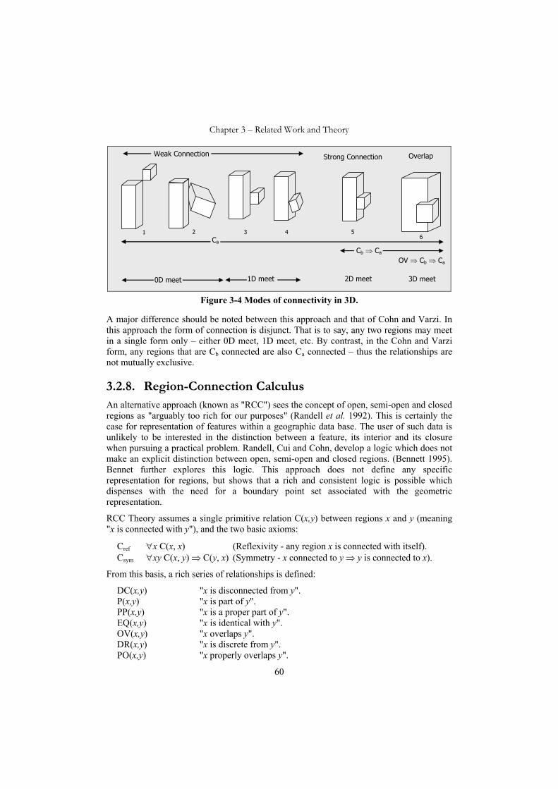
Chapter 3 – Related Work and Theory
60
Weak Connection
Ca Cb ⇒ Ca
OV ⇒ Cb ⇒ Ca
Strong Connection Overlap
0D meet 1D meet 2D meet 3D meet
1 2 3 4 56
Figure 3-4 Modes of connectivity in 3D.
A major difference should be noted between this approach and that of Cohn and Varzi. In this approach the form of connection is disjunct. That is to say, any two regions may meet in a single form only – either 0D meet, 1D meet, etc. By contrast, in the Cohn and Varzi form, any regions that are Cb connected are also Ca connected – thus the relationships are not mutually exclusive.
3.2.8. Region-Connection Calculus An alternative approach (known as "RCC") sees the concept of open, semi-open and closed regions as "arguably too rich for our purposes" (Randell et al. 1992). This is certainly the case for representation of features within a geographic data base. The user of such data is unlikely to be interested in the distinction between a feature, its interior and its closure when pursuing a practical problem. Randell, Cui and Cohn, develop a logic which does not make an explicit distinction between open, semi-open and closed regions. (Bennett 1995). Bennet further explores this logic. This approach does not define any specific representation for regions, but shows that a rich and consistent logic is possible which dispenses with the need for a boundary point set associated with the geometric representation.
RCC Theory assumes a single primitive relation C(x,y) between regions x and y (meaning "x is connected with y"), and the two basic axioms:
Cref ∀x C(x, x) (Reflexivity - any region x is connected with itself). Csym ∀xy C(x, y) ⇒ C(y, x) (Symmetry - x connected to y ⇒ y is connected to x).
From this basis, a rich series of relationships is defined:
DC(x,y) "x is disconnected from y". P(x,y) "x is part of y". PP(x,y) "x is a proper part of y". EQ(x,y) "x is identical with y". OV(x,y) "x overlaps y". DR(x,y) "x is discrete from y". PO(x,y) "x properly overlaps y".

Chapter 3 – Related Work and Theory
61
EC(x,y) "x is externally connected to y". TPP(x,y) "x is a tangential proper part of y". NTPP(x,y) "x is a non tangential proper part of y".
For example, P(x,y) is defined as ∀z[C(z,x) ⇒ C(z,y)] (x is part of y if any region z which connects with x must connect with y). These relations are pictured in Figure 3-5, where the most basic (disjunct) relations are shown at the bottom. Where two basic relations are connected to a higher level (such as TPP and NTPP being grouped under PP) this means that the lower two are refinements of the upper. For example P (part of) can be broken down into EQ or PP (proper part), which can be further broken down into TPP and NTPP. The topmost node, marked “T” is true for all regions. Note also that the -1 superscript in P-1, PP-1 etc. does not mean the inverse function (¬P etc.), it indicates the reverse – i.e. P-1(a, b) ⇔ P(b, a).
T
C DR
OV
P P-1
PP PP-1
TPP NTPP EQ NTPP-1 TPP-1 EC DC PO
a
a a a a
a a a
b
b b b b
b b b
NTPP(a,b) TPP(a,b) EQ(a,b) NTPP-1(a,b) TPP-1(a,b) EC(a,b) DC(a,b)
NTPP(b,a) TPP(b,a) ≡ ≡
PO(a,b)
Figure 3-5 The RCC relations (after Randell et al. 1992).
The further functions sum(x, y) (equivalent to x ∪ y), compl(x) (the complement of x), prod(x, y) (equivalent to x ∩ y), diff(x, y) (equivalent to x ∩ compl(y)), and US (the universal set), are similarly defined, but Bennett introduces a slightly different definition, which avoids the need for a NULL region (which however requires a sorted logic and some modification of the other definitions).
RCC originally added the further axiom – intended to ensure density of the regions:
∀x∃y [NTPP(y,x)] (loosely - every region contains a smaller region which is completely contained within it).
In discussing the possibility of atomic regions, Randell et al. (1992) showed that this axiom is redundant. Düntsch et al (2002), proved that it can be derived from the other RCC axioms. Thus the RCC is incompatible with an “atomic” space unless modified. The argument can be summarised as follows: Assume region A to be atomic (i.e. has no proper subset apart from the empty region OΦ). Let R be any other region R ≠ OΦ.

Chapter 3 – Related Work and Theory
62
If R ≠ A, then R is connected to A . If R = A, then R is connected to A . Thus ),(C),(C: ARARR ⇒∀ therefore AA⊆ .
The RCC theory is particularly attractive since it makes no assumptions about underlying representation beyond this set of axioms. However, a universal region which is not itself locally Euclidean can lead to connection definitions that diverge from "common sense" (Gotts et al. 1996).11 Thus some modification of the theory will be necessary where finite computational representations of regions are to be accommodated. In addition, the theory cannot be applied directly to finite representations as discussed above. This will be considered in detail in Section 6.1.1.
3.2.9. Proximity Space A closely related, alternative concept for the description of connectivity is that of the proximity space (Naimpally and Warrack 1970). Düntsch and Winter (2004) make the association between this and the Boolean connection algebra (see Section 3.2.4), and in fact, there is little difference apart from the symbolism used. The axioms given for a proximity space X with the proximity relation δ, regions A, B, C, E ⊆ X (the universal region) and empty region ∅ are (from Naimpally and Warrack):
(PS1) A δ B ⇒ B δ A (PS2) (A ∪ B) δ C ⇔ A δ C ∨ B δ C (PS3) A δ B ⇒ A ≠ ∅ ∧ B ≠ ∅ (PS4) A δ B ⇒ ∃ E: A δ E ∧ (X-E) δ B 12 (PS5) A ∩ B ≠ ∅ ⇒ A δ B.
The axiom PS4 is known as the "strong axiom", and a proximity space which does not satisfy this axiom is known as a weak proximity space. In effect, this axiom requires a dense, non-atomic space.
3.2.10. Boundary-free Representations Although the concept of a boundary as a point-set is useful in describing mathematical abstractions, it has no counterpart in the real world. “… it is nonsense to ask whether a physical object occupies an open or a closed region of space, or who owns the mathematical line along a property frontier” (Lemon and Pratt 1998 page 10). It might be thought that the concept of a boundary would be needed to ensure a definition of such concepts as tangential contact, but this is not the case. An alternate approach, from the algebras of connectivity, permits such predicates without invoking boundary point-sets.
11 Gotts et al (1996) gives an example of an especially constructed (non Euclidean) universal region that gives rise to unexpected definitions of "connected". Lemon & Pratt (1998) define a spatial region which, although it satisfies the definition of a regular set within a Euclidean universal region, is problematic. It is to avoid these issues that the latter paper introduces the "basic polygon", as a restriction of the regular set.
12 In this axiom, δ means “not δ”.

Chapter 3 – Related Work and Theory
63
One of the distinctions that can be made between the approaches of Egenhofer (Section 3.2.5) and Cohn and Varzi (Section 3.2.6) on the one hand and the region connection calculus (RCC) (Section 3.2.7) and proximity space (Section 3.2.9) on the other, is that the first two can be characterised as boundary representations, while the latter are boundary-free. The conventional, boundary description of a geometric object partitions space into the interior, boundary and exterior of that region. The concept of closure of a region is introduced – being the region with the boundary points included, as is the concept of interior – being the region with boundary points excluded. The alternative comes from the field of mereotopology.
3.2.11. Mereotopology There is a significant advantage in taking a mereological approach to spatial logic (Smith 1997), in that it avoids some of the distinctions between finite and infinite (smooth) sets. Thus, concepts such as "set contacts set" and "set includes set" move easily from the infinite to the finite realm13, whereas the definition of a region as a collection of points bounded by a boundary set of points does not.
Briefly, the distinction is that point-set topology defines regions as sets of points, with boundaries being a separate set of points, either included or not depending on whether the region is closed or open. The alternative, mereological approach is to treat the region as the fundamental concept, with the boundary arising as a natural consequence of the region being limited in extent (Borgo et al. 1996). The difficulty with point set topology as a tool for the representation of spatial regions is that a boundary must consist of a dense (possibly infinite) set of points, and so a distinction is created between the mathematical model and the computational representation. The boundary must be dense, because otherwise there will be gaps in the boundary, leaving neighbourhoods where the division of points into interior/boundary/exterior breaks down.
3.2.12. Imprecision and the Indiscernibility Relation In an attempt to allow for finite precision of operations, and finite accuracy and resolution, Worboys (1998) uses the concept of an "indiscernibility" relation ι where a ι b iff a and b are indiscernible within the representation. This is clearly not an equivalence relation, since a ι b, b ι c does not imply a ι c. (See discussion of Case 3 – the ISO 19107 Definition of equals() in Section 2.3). It does, however lead to a set of formal definitions for the concept of environments, or regions with indeterminate boundaries. It may be fruitful to approach the issue of the "tolerance" which is applied to many spatial calculations (Thompson and van Oosterom 2006a) in terms of the co-Heyting algebra formulation of Worboys (1998).
It is possible to define for points a, b that a ι b =def |ab| < δ or: a is indiscernible from b iff the distance between a and b (as calculated using finite precision arithmetic) is less than δ where δ is the tolerance. This would allow the question of "on the line" to be replaced by "indiscernible from the line". This of course allows the possibility that a point will be
13 Avoiding the problematic boundary point-sets, which as described in Section 1.5.5 may contain very few points in a finite representation.

Chapter 3 – Related Work and Theory
64
indiscernible from the interior of a region, and also indiscernible from the exterior of that region, which is acceptable in a co-Heyting algebra (Stell and Worboys 1997). While this does not provide any specific mechanisms for dealing with the sorts of issues documented in Chapter 2, it does allow a frame of reference for describing concepts such as the ISO 19117 definition of equals() as an indiscernibility rather than an equivalence relation. This will be considered further in Section 6.8.4.
3.2.13. Buffering of Regions In order to allow for imprecision in the definition of objects, and vagueness of definition of regions, many conventional GIS provide a buffering operation. The rationale is that when doing a search of objects in a region, it is better to include a few marginal objects than to omit any that should be included. For example, in determining which properties may be affected by a proposed activity, it is better to err on the side of inclusion.
O3∈R3
O4∈R4
O5∈R5
O1∈R1
O2∈R2
W
Figure 3-6 Imprecision in a region search.
Consider a search region which has been defined and measured to a limited accuracy (see Figure 3-6). Assume that to a 90% confidence, the position of all points defining the region is accurate to within δ of the correct position. Further, assume that objects Oi in the data base have accuracy such that their position is known to with γi, to a 90% confidence. If a search for objects is made based on this region, several cases can be identified, including:
An object can be confidently within the region – all points in the object Oi are within a buffered distance of δ+γi within the region. Call this set R1.
An object can be confidently contacting the region – some point(s) in the object Oi are within a buffered distance of δ+γi within the region. Call this set R2.
An object can be possibly within the region – all points in the object Oi are within a buffered distance of δ+γi outside the region. Call this set R3.

Chapter 3 – Related Work and Theory
65
An object can be possibly contacting the region – some point(s) in the object Oi are within a buffered distance of δ+γi outside the region. Call this set R4.
An object can be confidently excluded – no points of Oi are within a buffered distance of δ+γi outside the region. Call this set R5.
In practice, a particular search would make use of a subset of these regions. For example, a request might be made for “all objects within the region”. This would be accomplished by determining R1 (objects confidently within), R3 (objects possibly within) and 3R (objects not possibly within). Alternatively, a request for “all objects contacting the region”, which would use R2, R4 and R5.
In the simple case being illustrated in Figure 3-6, it has been assumed that all objects in the database have an easily assigned positional accuracy γi (indicated by shading surrounding the region). In real cases this is more complex due to the nature of the accuracy of extended features.
In practice, there are some significant difficulties in applying this kind of approach. The approach frequently taken is that, rather than searching for objects within a defined region W, the region buffered by γ+δ where γ = max(γi) is substituted. This is justified by the assumption that any object falling outside this buffer is unlikely to be affected. It is also common to use a “negative buffer” when only those objects that belong to R1 are wanted. The approach to buffering a region often is accomplished by generating a polygon approximation of a curved buffer around external vertices, which is quite appropriate for the vast majority of situations where a positive buffer is needed, but the negative buffer is less satisfactory.
W
O3
p
O1
O2
Figure 3-7 Positive and negative buffering of a region.
For example, in Figure 3-7, a positive buffer around region W will include regions O1, O2 and O3, as possibly intersecting with W. On the other hand, all will be excluded by the negative buffer shown. This is not correct in the case of O3 which has a high likelihood of intersecting W. This situation can apply whenever acute angles such as that at p occur in a defined region.

Chapter 3 – Related Work and Theory
66
3.2.14. Fuzzy Logic and Fuzzy Regions A region O in a topological space X can be viewed as a Boolean valued function f(X)→{0,1}. That is to say, for every point p∈X, a value of 0 or 1 can be assigned with 0 (false) meaning p ∉ O, and 1 (true) meaning p ∈ O. This crisp formulation can be replaced by a fuzzy logic formulation, replacing the Boolean valued function with a real valued function μ(X) → [0, 1]. That is, for every point p∈X, a value within the closed interval [0, 1] is assigned (Dilo 2006). The interpretation of this function is that a point for which the value is zero is certainly outside the set, a value of one indicates certainty of inclusion, with all intermediate values indicating the degree of certainty. The support set of a fuzzy set is defined as the set of points for which μ(x) > 0, while the core is the set for which μ(x) = 1. These are both conventional sets.
Ideally, this could be viewed as a probability density function, with the value at any point being the probability that the point belongs to the region. For example, if a 1 dimensional region is considered, say the region O = {x ∈ RR1 : x ≥ a}, i.e. those real numbers ≤ a. If the determination of the value of a is imprecise and this imprecision is the result of a large number of unrelated factors, by the central limit theorem the distribution of the measurement approaches the normal distribution. Therefore the probability density function of a (assuming the true value of a is μ) approximates to:
2
2
2)(
21)( σ
μ
πσ
−−
=a
eaf
where σ is the standard deviation of the measurement (Hogg and Craig 1965).
This means that the probability that a point at position x is within the region O would be:
dteOxprx at
∫∞−
−−
=∈ 2
2
2)(
21)( σ
πσ
0
1
a
pr(x∈O) σ
σ’
Figure 3-8 1D fuzzy region, interpreted as a probability density function.
In Figure 3-8, the fuzzy interpretation of region O is depicted as a probability density function, with a standard deviation of σ. For comparison, a function with a larger standard deviation σ’ is drawn as a dashed line. This would be ideal as a representation of an imprecise region, except for some practical considerations:
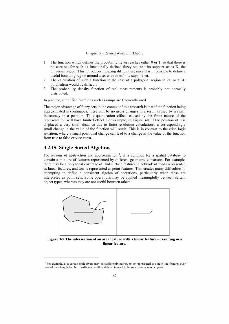
Chapter 3 – Related Work and Theory
67
1. The function which defines the probability never reaches either 0 or 1, so that there is no core set for such as functionally defined fuzzy set, and its support set is X, the universal region. This introduces indexing difficulties, since it is impossible to define a useful bounding region around a set with an infinite support set.
2. The calculation of such a function in the case of a polygonal region in 2D or a 3D polyhedron would be difficult.
3. The probability density function of real measurements is probably not normally distributed.
In practice, simplified functions such as ramps are frequently used.
The major advantage of fuzzy sets in the context of this research is that if the function being approximated is continuous, there will be no gross changes in a result caused by a small inaccuracy in a position. Thus quantization effects caused by the finite nature of the representation will have limited effect. For example, in Figure 3-8, if the position of a is displaced a very small distance due to finite resolution calculations, a correspondingly small change in the value of the function will result. This is in contrast to the crisp logic situation, where a small positional change can lead to a change in the value of the function from true to false or vice versa.
3.2.15. Single Sorted Algebras For reasons of abstraction and approximation14, it is common for a spatial database to contain a mixture of features represented by different geometric constructs. For example, there may be a polygonal coverage of land surface features, a network of roads represented as linear features, and towns represented as point features. This creates many difficulties in attempting to define a consistent algebra of operations, particularly when these are interpreted as point sets. Some operations may be applied meaningfully between certain object types, whereas they are not useful between others.
Figure 3-9 The intersection of an area feature with a linear feature – resulting in a
linear feature.
14 For example, at a certain scale rivers may be sufficiently narrow to be represented as single line features over most of their length, but be of sufficient width and detail to need to be area features in other parts.

Chapter 3 – Related Work and Theory
68
Consider the intersection and union operations. These are amongst the most fundamental of all the operations on spatial objects, but have different criteria where mixed geometries are concerned. The intersection of an area feature with a point, linear or area feature is quite a meaningful operation, for example in Figure 3-9, where the intersection of the lightly shaded region on the left is formed with the linear feature. The result, as shown in the right pane is a linear feature.
Forming the union of a mixture of geometry types is problematic, as can be seen in Figure 3-10. Here, in contrast with the intersection which produced a single simple geometry type, the result is a single feature of mixed geometry type, or of generic type.
Figure 3-10 The union of an area feature with another geometry type.
Many commercial systems allow this mixed geometry type as a primitive for just this reason, and in fact it would be a marketing disadvantage not to provide the type, but there are further complications that result. It is highly desirable that a system should provide a subtraction operation15 (e.g. find the area of the local government region not under cultivation), but this is not readily accomplished where mixed geometries are allowed. For example, in Figure 3-11, the mixed geometry object (from Figure 3-10) is subtracted from the simple area feature. The result is a set of points within a polygon, but with holes that are not simply represented. (In this case, an infinitely thin line which is not part of the region).
Figure 3-11 A mixed geometry subtracted from an area feature.
15 It can be argued that an inverse operation is not really necessary (as the universe excluding the points within the region), but a subtraction operation is very useful.

Chapter 3 – Related Work and Theory
69
In order to ensure closure of the operations of union, intersection and subtraction of mixed geometries, it is necessary (in 2D) to provide a primitive which consists of a collection of areas, lines and points, with holes that can be areas, lines and points.
This is known as a single sorted algebra, since there is only one object sort (called “geometry”, which is a complex collection of primitives as described above), and each operation must be able to be applied to any objects of this sort.
3.2.16. Many Sorted Algebras The alternative approach is to use a sorted algebra, where operations may apply only to certain restricted sorts of objects. It is possible for different operations to have the same name. E.g. the intersection of two area features has the same name ("intersection") as the intersection of two linear features.
A sorted algebra has a more complex definition and structure, but has advantages in the development of a simplified implementation, since the range of operations that need to be programmed has been clearly defined, and is restricted in scope. For an example of a many sorted algebra, see the discussion of the ROSE algebra in Section 3.4.5.
Applied to the representation of spatial data, a many sorted algebra allows each sort of geometric item to participate in different operations. For example, the union operation might be defined for pairs of multi-area features, pairs of multi-line features and pairs of multi-point features (the detail is not important here), without necessarily allowing the union of a multi-area feature with a multi-line16. This fits well with the object-relational approach to database management, where a family of functions or predicates with the same name are polymorphically associated with different object types (Stonebraker and Moore 1996).
This might appear to be restrictive, but in practice it is not. Where an operation between particular sorts of objects is meaningful it can be defined, but where it is not meaningful it is not defined, and so there are no problematic operations to be implemented (such as area feature minus linear feature).
3.3. Precision of Calculations and Representation Since a real number cannot be directly stored as a value, typically either integer or floating point representation will be used (see Section 1.5). This inevitably introduces an approximation on initial data capture, and rounding errors in individual calculations. Although the errors thus introduced can be made small by using high precision calculation, they remain significant as "it is impossible to separate the geometry from the topology since arbitrarily small geometry errors can later cause topology errors" (Franklin 1984 page 191).
16 This is not to say that union of mixed object sorts cannot or should not be allowed, but that a many sorted algebra allows detailed definition of exactly which operations are allowed and the sorts to which they can be applied.
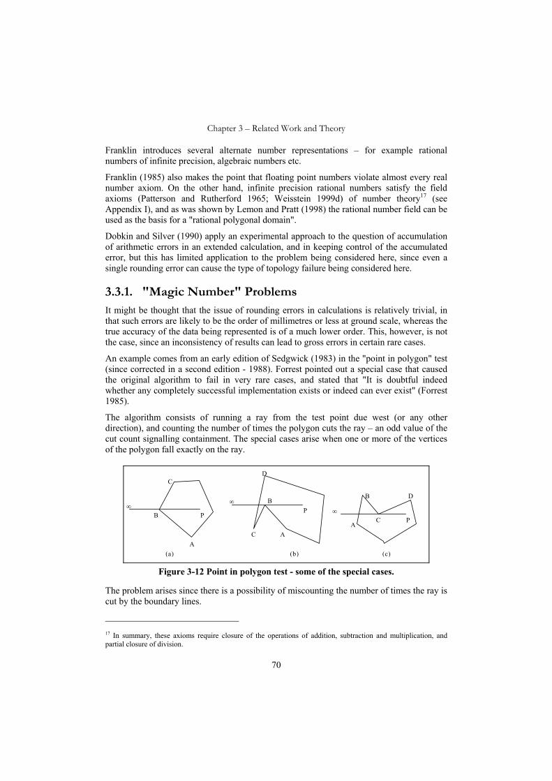
Chapter 3 – Related Work and Theory
70
Franklin introduces several alternate number representations – for example rational numbers of infinite precision, algebraic numbers etc.
Franklin (1985) also makes the point that floating point numbers violate almost every real number axiom. On the other hand, infinite precision rational numbers satisfy the field axioms (Patterson and Rutherford 1965; Weisstein 1999d) of number theory17 (see Appendix I), and as was shown by Lemon and Pratt (1998) the rational number field can be used as the basis for a "rational polygonal domain".
Dobkin and Silver (1990) apply an experimental approach to the question of accumulation of arithmetic errors in an extended calculation, and in keeping control of the accumulated error, but this has limited application to the problem being considered here, since even a single rounding error can cause the type of topology failure being considered here.
3.3.1. "Magic Number" Problems It might be thought that the issue of rounding errors in calculations is relatively trivial, in that such errors are likely to be the order of millimetres or less at ground scale, whereas the true accuracy of the data being represented is of a much lower order. This, however, is not the case, since an inconsistency of results can lead to gross errors in certain rare cases.
An example comes from an early edition of Sedgwick (1983) in the "point in polygon" test (since corrected in a second edition - 1988). Forrest pointed out a special case that caused the original algorithm to fail in very rare cases, and stated that "It is doubtful indeed whether any completely successful implementation exists or indeed can ever exist" (Forrest 1985).
The algorithm consists of running a ray from the test point due west (or any other direction), and counting the number of times the polygon cuts the ray – an odd value of the cut count signalling containment. The special cases arise when one or more of the vertices of the polygon fall exactly on the ray.
PP
(a) (b)
∞∞
A
B
C
C
B
A
D
A
B
C
D
P∞
(c)
Figure 3-12 Point in polygon test - some of the special cases.
The problem arises since there is a possibility of miscounting the number of times the ray is cut by the boundary lines.
17 In summary, these axioms require closure of the operations of addition, subtraction and multiplication, and partial closure of division.

Chapter 3 – Related Work and Theory
71
P P
(a) (b)
∞∞
A
BC CB
AD D
P ∞
(b) Figure 3-13 Point in polygon test - more complex special cases.
As it happened, Forrest was wrong in this particular case, and a completely satisfactory algorithm does exist (Sedgwick 1988). However examples of this class of error are still quite common in commercial spatial software, and are given the colloquial name "magic number problems". They are categorised by the extreme rarity of failure (often with a probability of about 1:109 of occurring in any individual case), and caused by accidental co-incidences of values. This rarity makes the removal of these "bugs" by classical "debugging" techniques totally impractical, based on achievable test data quantities, and often the problems remain undetected or are ignored.
Note – increasing the precision of calculations does not solve this type of problem; it merely makes its occurrence less frequent. It also makes this kind of problem less likely to be found by testing.
3.4. The Digital Representation The majority of the literature on the representation of spatial information within computers has, as this chapter shows, been in the realm of the mathematical model, with such issues as rounding, imprecision and calculation errors being largely left to the programmer. This section discusses the smaller body of literature that deals directly with the finite precision of the computer representation.
3.4.1. Simulation of Simplicity In an attempt to remove problems associated with rounding and accidental coincidences of numeric values (see Section 3.3.1), the technique of "Simulation of Simplicity" has been developed (Edelsbrunner and Muecke 1988). This uses the concept of a perturbation of the case in question by a small amount, so as to prevent any degenerate cases such as the co-incidence of latitude cited by Forrest (the “magic number” problems discussed in Section 3.3.1). This perturbation is allowed to be smaller than the minimum resolution that can be represented in the digital number system, and is therefore not actually included in the calculations, but proves that the algorithm is correct.
As a simple example, returning to the problem of determining if a point is within a polygon (in 2D), the problem of “is point p = (x, y) within the polygon”, the problem is restated as “is point p = (x, y+ε) within the polygon”. If ε is smaller than the grid interval, then this is an equivalent problem.

Chapter 3 – Related Work and Theory
72
v1
A
v2
p = (x, y)
Figure 3-14 Using "Simulation of Simplicity" to solve the point in polygon problem.
One procedure for determining whether a point is within a polygon is to run a ray to the west and count the times the polygon boundary cuts the ray. An odd number of cuts indicates that the point is within the polygon. Referring to Figure 3-14, if point p had been used, and a ray run to the west, the ray would have passed through vertices v1 and v2, creating significant special case processing. (For more examples of this issue, and the complexity of the special cases, see Section 3.3.1). By using point p’, by contrast, no vertices can ever possibly lie along the ray. The edges that meet a vertex v1 will not be counted, while those at v2 will both be counted – so that the parity of the answer will be correct. If the value of ε is allowed to approach zero, then p’ approaches p.
In this case, a simple solution is available which does not include ε in the calculation, but in the more general cases, additional resolution is needed in the calculations. Edelsbrunner and Muecke postulate a series of primitive functions which parallel the usual mathematical functions, but which take account of this perturbation (and thus hide the details from the casual user). For example, in place of the “less than” relational predicate, a “Smaller” function is defined which eliminates the equality case. Thus ¬a.Smaller(b) ⇒ b.Smaller(a). These have additional precision requirements for internal calculations.
While an extremely powerful technique in tackling individual problems, "Simulation of Simplicity" is difficult to apply to "componentised" software, and particularly where the nesting of functions is not constrained.
3.4.2. Milenkovic Normalisation
Milenkovic defines a set of normalisation rules, based on a parameter ε which is chosen using the criterion that the "distance between a point and a line segment can be calculated with accuracy ε10
1 " (Milenkovic 1988 page 382). Three of the relevant rules are:
1. No two vertices are closer than ε. 2. No vertex is closer than ε to an edge of which it is not an endpoint. 3. No two edges intersect except at their endpoints

Chapter 3 – Related Work and Theory
73
For spatial data that satisfies these rules, a random relative movement of points which does not exceed ε will not result in an invalid geometry (by the OGC definition of "valid"). This clearly prevents interchange problems like those illustrated in the Case Studies 2, 4, 6 and 12 (Sections 2.2, 2.4, 2.6 and 2.12), provided the magnitude of any perturbation of the point positions is < ε. On the other hand, if data positions are perturbed by a random amount up to a maximum distance of δ, on arrival, the data is no longer guaranteed to be valid at a tolerance of ε, but at a smaller tolerance ε-δ.
Thus it is not practical to specify a particular tolerance value ε, and promulgate it as a universal definition of validity, since any perturbation in transmission will potentially cause the validity test (at tolerance ε) to fail. A preferred practice is to define the “robustness” of the data – as the largest possible value of ε for which the data is Milenkovic normal, allowing transmission if the transmission accuracy δ is better than ε, and contracting to deliver the data as “Milenkovic normal at ε-δ” (Thompson and van Oosterom 2006a).
Milenkovic normalisation solves many issues of failure of operations, but only where the geometric constructs have been normalised prior to those operations. In addition, normalisation of a construct exaggerates the movements of points such as seen in Case 1 (Section 2.1) since the minimum distance ε must be ten times the grid spacing, and so the process itself may not be associative. In addition, the process can be difficult, with the selection of tolerance parameters not being a trivial exercise.
3.4.3. Realms A direct approach was taken by Güting and Schneider (1993) using the concept of "realms", investigating in detail the properties of the representation itself, rather than the mathematical abstraction. Realm objects are defined in terms of the finite digital representation. In effect, all feature representations on entry to the database are compared with all existing representations in the vicinity, and the points of intersection calculated. This may be an expensive operation, but results in a closed and correct logic for the operations between the objects. Many of the cases discussed in Chapter 1 are successfully handled by this approach. (The relationship between this approach, and the approach being suggested in this proposal will be discussed in more detail in Chapter 9).
This approach is taken further by Güting et al (1995) with the definition of a complete, numerically robust algebra ("ROSE") (see Section 3.4.5). These papers are restricted in scope to 2D, but there is no apparent reason why the "realms" approach should be thus limited. There would, however, be a significant increase in complexity involved in extending to the additional dimension.
In order to prevent the problems such as non-associativity of operations (see Section 2.1 - Case 1) and other such problems where a movement generated by the calculation of points can cause earlier results to become invalidated, the realms approach uses a technique of trapping a line within its envelope (Green and Yao 1986) – introducing extra points if necessary.
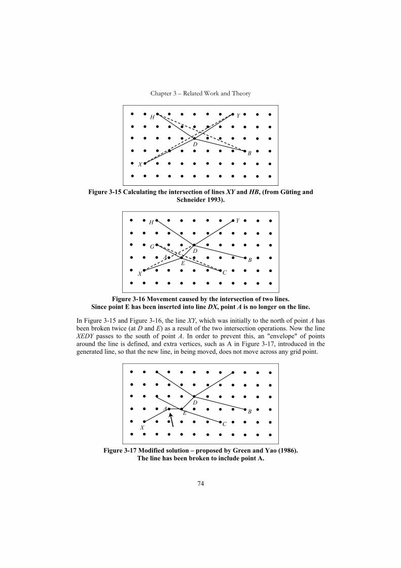
Chapter 3 – Related Work and Theory
74
D B
X
Y H
Figure 3-15 Calculating the intersection of lines XY and HB, (from Güting and
Schneider 1993).
A D
B E C X
Y H
G
Figure 3-16 Movement caused by the intersection of two lines.
Since point E has been inserted into line DX, point A is no longer on the line.
In Figure 3-15 and Figure 3-16, the line XY, which was initially to the north of point A has been broken twice (at D and E) as a result of the two intersection operations. Now the line XEDY passes to the south of point A. In order to prevent this, an "envelope" of points around the line is defined, and extra vertices, such as A in Figure 3-17, introduced in the generated line, so that the new line, in being moved, does not move across any grid point.
A D
B E
C X
Figure 3-17 Modified solution – proposed by Green and Yao (1986).
The line has been broken to include point A.

Chapter 3 – Related Work and Theory
75
Y
X
Figure 3-18 Envelope of points surrounding a line.
Figure 3-18 shows the envelope of points that surround a line. These comprise all the points adjacent to the line on each side – that is, all points within one grid interval. These are the points that could become intersection points of this line with any other line, and they mark the greatest distance the line can be displaced from its original position (the line remains within the shaded area no matter how many intersection operations occur).
This provides a solution, but at the cost of extra complexity in the final geometry. Note firstly that the introduction of a point in a "straight" line may involve the introduction of several "envelope points" as vertices in the line. It is not clear just how many points could be required, and this is an area that has been identified as requiring some further research. On the other hand, note that the wanderings of a line caused by these operations cannot exceed the grid size, thus a limit has been set on any "creeping" of the data. It also should be noted that the final result is dependent on the order of formation of the intersections:
Y
X
C
D
A
B
Figure 3-19 Intersecting line XY with line AB and then line CD.
For example, in Figure 3-19 the line XY has been moved to the north, while in Figure 3-20 it has moved to the south. The total movement is less than a grid interval, and so is within the requirements of the realms approach.

Chapter 3 – Related Work and Theory
76
Y
X
C
D
A
B
Figure 3-20 Intersecting line XY with line CD and then line AB.
In three dimensions, the situation becomes more complex. Presumably, the same form of envelope would be defined, and any line or plane surface would be similarly constrained.
A
B
C
a
b
c
Figure 3-21 Intersecting plane surface A with the plane surfaces B and C.
Consider the case depected in Figure 3-21, in which the plane surface A is being intersected with surfaces B and C (which are assumed to be coplanar). Even in this simple case, snapping of the calculated points a and b may cause envelope points to be generated in the perimeter of A. Similarly, the calculation of c may cause point generation of extra points in ac and bc. Even more, the movement of the perimeter of A will cause movement of the plane itself, so that envelope points may be contacted by the plane A itself.
The points marked with an “×”, in Figure 3-22 are envelope points of A contacted by the plane, and now included in the surface definition. The fine lines are the "crease lines" caused by these points. (Only surface A has been used to illustrate the "creasing" effect). This is not to say that the approach will not work in 3D. It certainly will, but the complexity of the resultant objects would be expected to increase dramatically over the 2D case.

Chapter 3 – Related Work and Theory
77
A
B
C
a
b
c
Figure 3-22 Additional envelope points included in lines and surfaces.
3.4.4. The Dual Grid The “dual grid” (Lema and Güting 2002) defines points, lines and regions (in 2D) in terms of points with rational number coordinates. In order to avoid the movement of line segments when they are intersected with other line segments (as described above in Section 3.4.3), two grid intervals are used. The coarser grid is used to define any points that can be the end points of a line segment, while any point that represents the intersection of two line segments can be represented by coordinates on the finer grid. This finer grid is based on rational numbers, but it should be noted that these rational numbers are of finite precision. See Section 4.4 for a definition of domain-restricted rational numbers.
For example, returning to the example shown in Figure 3-16, the dual grid approach does not force the points of intersection to fall on the points of the same grid as used to define the lines. As can be seen in Figure 3-23, the points of intersection (shown as open circles) are between the grid points, and are exactly calculated as higher precision rational numbers. This means that, again returning to the earlier example, point A remains in the same relationship to the line as before calculation of the intersection. The dual grid has, like the realms approach, been shown to implement the ROSE algebra.
A
D
B E
C
H
G
X
Y
Figure 3-23 The example from Figure 3-16 as represented in the dual grid.
The points of intersection of lines which do not fall on the first level grid points cannot be used as the endpoints to define new lines, as this would lead to unbounded precision

Chapter 3 – Related Work and Theory
78
requirements. For example, in Figure 3-23, a line cannot be defined with point D as an endpoint.
There is some additional complexity involved in extending the dual grid approach to 3D, which will be discussed in Section 7.7.1.
3.4.5. The ROSE Algebra The ROSE algebra (Güting and Schneider 1995) is a many sorted algebra (see Section 3.2.16) designed for geographic information. It provides for geometries which are collections either of points, lines, or regions18, with the operations being defined for these types, where applicable. The basic object, the realm, which is used to construct all geometric primitives, is a set of points which lie on a discrete grid, and non-intersecting lines whose endpoints also lie on this grid. All intersections between line segments are assumed to be pre-calculated at the time the representations enter the database, or when updates are made. “…there are never any new intersection points computed in query processing.” (Güting and Schneider 1993).
For example, there is an operation union19 defined on two regions values, which returns a value of type regions. (The return region is the area that is within either region). Implicit in this is a form of normalisation, where the union of two regions is actually defined as the closure of the union of the interior of those regions – thus eliminating any lines or points from the result. While there is no mixed geometry type, there are “kinds” such as GEO, which allow for polymorphic operations. Thus is possible to define the inside predicate as operating on one object of type GEO (points, lines or regions) and one object of type regions. The return value is true if the object of type GEO is within the object of type regions.
There are four classes of operations:
Spatial predicates (e.g. inside, adjacent), Operations returning spatial objects (e.g. intersection), Operations returning numbers (e.g. length), Operations on sets of objects (overlay, fusion).
It is significant that there is a subtraction operation (difference), returning the difference between two objects of the same geometric type, and that the intersection operation comes in several varieties – for example, lines intersecting lines give points as a result, regions intersecting regions give regions as a result. Regions intersected with lines give lines. Intersection is defined on the realms that define a region, so that the intersection of two regions is always a region etc., and cannot ever degenerate into the points or lines of contact. By contrast, plus (union) and minus (difference) are more restricted, only applying to objects of the same sort. Also of significance are the overlay, sum and fusion
18 The algebra as defined is limited to 2D, but would readily extend to 3D or more without requiring any new concepts. 19 The use of bold typeface, italics and underlining in this section follows the usage in Güting and Schneider (1995b).

Chapter 3 – Related Work and Theory
79
operations. Overlay calculates the superimposition of two partitions of the plane, breaking all regions into the smallest common regions (e.g. overlaying administrative districts onto vegetation types). Sum forms the union of all regions in a set, and fusion combines regions according to some common attribute value (e.g. a collection of cadastral parcels could be fused into regions of the same town planning code).
It might be thought that this algebra is more restrictive and less flexible than the single sorted algebra discussed above, but this would be to miss the point. The operations that are not permitted in the ROSE algebra are not useful, and can produce positively misleading results. For example, a calculation of the area of a mixed object such as those in Figure 3-11 cannot be expected to give a meaningful result. Likewise, the area of a linear feature, or the length of an area feature cannot return useful results.
As was described above, the ROSE algebra also has the track record of having been implemented in both the realms approach (Section 3.4.3) and in the dual grid approach (Section 3.4.4).
3.4.6. Infinite Precision Rational Numbers The "complete calculus for rational polygonal regions" (Lemon and Pratt 1998) suggests an approach built on rational numbers as a basis. "Infinite precision rational numbers", are also suggested by Franklin (1984). The biggest advantage of infinite precision rational numbers is that they satisfy the mathematical field axioms (see Section 1.5.3, and Appendix I.1). That is to say, they form a number system which is closed under addition and multiplication, and each number except zero has an additive and a multiplicative inverse (Patterson and Rutherford 1965; Weisstein 1999d). Schneider and Praing (2006) develop a rigorous logic known as “spatial algebra 2D” (SPAL2D), based on this kind of representation. They describe the form of number as “arbitrary, finite length … limited by main memory”.
Infinite precision rational numbers can in fact be represented digitally20. For example, the Java package Java.math (Sun 2003) (amongst other environments) provides data types of "BigInteger" and "BigDecimal", which allow arithmetic to be performed on numbers of arbitrary magnitude up to the memory size available. An infinite precision rational number could be defined as the ordered pair of "BigInteger" variables (P, Q), where Q > 0, and given the interpretation P/Q. A set of arithmetic operations can be defined such as addition and multiplication:
( )1
21
1
1221 ,2211 ),(),(F
QQF
QPQPdefQPQP ××+×=+ (f3.1)
where F1 = largest common factor of (P1×Q2+P2×Q1)and Q1×Q2. ( )2
21
2
21 ,2211 ),(),(F
QQF
PPdefQPQP ××=× (f3.2)
where F2 = largest common factor of P1×P2 and Q1×Q2.
20 This is not, strictly speaking, true, but can be treated as being so for this purpose – see Section 1.5.4.

Chapter 3 – Related Work and Theory
80
Note that the worst case in this definition is when the largest common factor of P1×P2 and Q1×Q2 is 1. If P1, P2, Q1 and Q2 are random numbers, the probability of P1 and Q1 being relatively prime is about 0.6079 (actually 6/π2 (Castellanos 1988; Weisstein 2006b)), the probability of P1 and Q2 is also about 0.6079.
Therefore the probability of P1 and Q1×Q2 having a common factor is approximately: 0.3921 + 0.6079 * 0.3921 = 0.6305. (The probability of P1 and Q1 having a common factor plus the conditional probability that P1 and Q2 have a common factor given that P1 and Q1 do not).
Therefore the probability of P1×P2 and Q1×Q2 having a common factor is similarly about: 0.6305 + 0.3695 * 0.6305 = 0.8634
That is to say, in about 14% of cases, the common factor in the above definition can be expected to be one, and no reduction in storage requirements is possible.
This highlights the disadvantage of the infinite precision rational number approach in that any operation between rational numbers is highly likely to increase the precision requirements of the result. Thus after a long series of operations, the storage requirements of a representation increase (without bound), and processing time requirements for further operations increase (also without bound). Note that with numbers of the size found in spatial data – where 9 digits resolution is commonplace, the numerators and denominators can become very large indeed. The characteristic of unlimited rational numbers is that each time a pair of numbers is added, subtracted or multiplied, the denominator is potentially the product of both denominators. For example if common factors are not applied in equations f3.1 and f3.2 they become:
(P1, Q1) + (P2, Q2) = (P1 × Q2 + P2 × Q1, Q1 × Q2) (P1, Q1) × (P2, Q2) = (P1 × P2, Q1 × Q2)
A common factor can be found, using the Euclidean Algorithm (Courant and Robbins 1941; Weisstein 2006a) which allows the fraction to be simplified in some cases, but typically, the precision requirements grow linearly (in terms of number of bits required in the result) with the number of operations executed.
For example, in order to calculate a plane that passes through three (non collinear) points (x1, y1, z1), (x2, y2, z2), (x3, y3, z3), the formula can be given as (Weisstein 2002a):
0
1111
333
222
111 =
zyxzyxzyxzyx
(f3.3)
That is to say, in the form Ax + By + Cz + D = 0, with A, B, C, D integers,
A = y1 z2 - y1 z3 + y2 z3 – y2 z1 + y3 z1 – y3 z2. (f3.4)
Where all points have integer coefficients, in the range –M to M, this means that A is an integer in the range -6M2 to 6M2. Similarly, B and C are in the same range, and
D = x1 (y2 z3 - y3 z2) + x2 (y3 z1 – y1 z3) + x3 (y1 z2 – y2 z1). (f3.5)
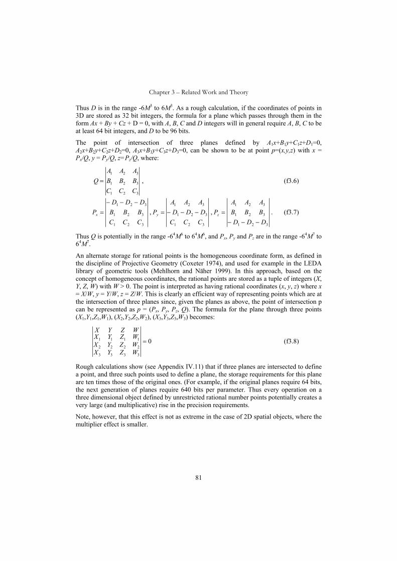
Chapter 3 – Related Work and Theory
81
Thus D is in the range -6M3 to 6M3. As a rough calculation, if the coordinates of points in 3D are stored as 32 bit integers, the formula for a plane which passes through them in the form Ax + By + Cz + D = 0, with A, B, C and D integers will in general require A, B, C to be at least 64 bit integers, and D to be 96 bits.
The point of intersection of three planes defined by A1x+B1y+C1z+D1=0, A2x+B2y+C2z+D2=0, A3x+B3y+C3z+D3=0, can be shown to be at point p=(x,y,z) with x = Px/Q, y = Py/Q, z=Pz/Q, where:
321
321
321
CCCBBBAAA
Q = , (f3.6)
3
3
3
2
2
2
1
1
1
CBD
CBD
CBD
Px
−−−= ,
3
3
3
2
2
2
1
1
1
CD
A
CD
A
CD
APy −−−= ,
3
3
3
2
2
2
1
1
1
DBA
DBA
DBA
Pz
−−−= . (f3.7)
Thus Q is potentially in the range -64M6 to 64M6, and Px, Py and Pz are in the range -64M7 to 64M7.
An alternate storage for rational points is the homogeneous coordinate form, as defined in the discipline of Projective Geometry (Coxeter 1974), and used for example in the LEDA library of geometric tools (Mehlhorn and Näher 1999). In this approach, based on the concept of homogeneous coordinates, the rational points are stored as a tuple of integers (X, Y, Z, W) with W > 0. The point is interpreted as having rational coordinates (x, y, z) where x = X/W, y = Y/W, z = Z/W. This is clearly an efficient way of representing points which are at the intersection of three planes since, given the planes as above, the point of intersection p can be represented as p = (Px, Py, Pz, Q). The formula for the plane through three points (X1,Y1,Z1,W1), (X2,Y2,Z2,W2), (X3,Y3,Z3,W3) becomes:
0
3333
2222
1111 =
WZYXWZYXWZYXWZYX
(f3.8)
Rough calculations show (see Appendix IV.11) that if three planes are intersected to define a point, and three such points used to define a plane, the storage requirements for this plane are ten times those of the original ones. (For example, if the original planes require 64 bits, the next generation of planes require 640 bits per parameter. Thus every operation on a three dimensional object defined by unrestricted rational number points potentially creates a very large (and multiplicative) rise in the precision requirements.
Note, however, that this effect is not as extreme in the case of 2D spatial objects, where the multiplier effect is smaller.

Chapter 3 – Related Work and Theory
82
3.4.7. Interval Arithmetic Franklin (1984) discusses the use of “interval arithmetic” in the context of preventing topological failures caused by finite precision calculations. In effect, this approach represents a real number computationally as an ordered pair of floating point numbers, representing the minimum and maximum possible value the real number could have. When any operation is carried out between two variables, the widest range of values that could be generated as a result is determined, allowing for inaccuracies in the calculation and the original range of numbers.
For example, assuming that only 3 decimal digits are available for calculation, a variable might be intended to have the value π but be represented as (3.141, 3.142). The variable r might be measured, and fall in the range (1.245, 1.246), so that calculation of π.r using interval arithmetic would give the result (3.910, 3.915). The first integer represents the product of the minimum values, rounded down to three decimal places. The second is the product of the maximum values, rounded up.
Notice that this approach is rigorous, but pessimistic. (In the above example, the range of imprecision has increased from 0.001 to 0.005 in a single operation). After a number of operations, the true result will be guaranteed to be within the calculated interval, but the theory of rounding would have led to significantly smaller estimates of the likely error (Goldberg 1991).
Applied to spatial data, appropriately used, this approach will ensure that no topological failures will ever occur undetected, provided that the “worst cases” for every coordinate value can be determined. This is not always obvious (see Figure 3-24), and so there is some scope for this to be combined with the robustness measure approach discussed in Section 2.4. As a first test, a tolerance can be determined from the intervals in each point coordinate value, and used as the parameter in a test for Milenkovic normalisation. If this succeeds, the geometry is valid, and there is no need for more complex calculations.
4
1
2
3
5
6
7
8 9
Figure 3-24 Interval arithmetic and geometric validity.
As an example of the difficulty in determining the worst cases in interval arithmetic, consider point 4 in Figure 3-24. In this figure, each point is surrounded by a rectangle that represents the interval of its coordinate values. If points 1 and 2 happen to take their minimum values, then the worst case for point 4 is the maximum values of its coordinate

Chapter 3 – Related Work and Theory
83
intervals. On the other hand, it also has a worst case on its southern limit (risking a clash with point 9), and its north-western corner (risking a clash with point 6).
Note that the interval arithmetic range of accuracy is not to be confused with the actual positional accuracy of the original data. The range of values in interval arithmetic is a “hard edged” range. There is no possibility that the true result could fall outside the limit set by the ordered pair of floating point numbers. In general, the measurement of a real-world value generates a number with a certain accuracy, often with a normal distribution (Fraser 1958). This, by contrast is a “soft edged” range, and there is a non-zero probability that the true value may be outside the stated range.
For example, if an object is measured at 134m ± 0.5m, it cannot be claimed that the object cannot be less than 133m long. Frequently a confidence limit is stated – for example a 95% confidence means that, on average about 5% of measurements will be outside the stated accuracy range.
3.4.8. Constraint Databases This is a relatively new approach (Grumbach and Jianwen 1997), extending the well accepted relational database model, which can be applied to spatial data by recognising that a geographic region can be encoded as a set of constraints which are equations or inequalities defining the boundaries of the region (Kanellakis and Golding 1994; Kanellakis et al. 1995). Each constraint can be a linear or other inequality which constrains the region in space (similar to the concept of "half space" to be introduced in Chapter 4). These constraints can be combined using “and” and “or” conditions to define a spatial region. (e.g. "Brussels = (y≤13) ∧ (x≤11) ∧ (y≥12) ∧ (x≥10)").
A linear constraint model has been proposed by Gunther (1988) and by Vandeurzen et al. (2001), in which geometric objects are represented as a finite sum of convex "cells" each of which is a finite intersection of half planes. Although using the language of 2D, this approach has no dimensionality limitations. It can further be shown that it is topologically correct in its results. The representation can also be made robust. If the constraints are chosen carefully, small changes in the constants will cause commensurately small movements of the positions of the boundaries. Furthermore, these movements will not in any circumstances cause a region to become invalid.
There are many variants on the constraint approach, depending on the complexity of the allowable constraints - linear, polygonal, non-linear or semi-linear (Vandeurzen et al. 2001), and no clear indication of which varieties are the most appropriate to a specific application. Nevertheless, a prototype known as "Dedale" has been built, and proved to be efficient in the 2D case, and showing promise for extension into 3D and higher dimensions (Grumbach et al. 1997; Grumbach et al. 1999; Grumbach et al. 2000).
There is a strong relationship with the current research and the linear constraint model, and this will be discussed in some detail in Section 6.9.

Chapter 3 – Related Work and Theory
84
3.5. Conclusions This chapter has addressed existing literature pertinent to this research subject, revealing the situation of a well understood and researched theory of space, usually defined in terms of an infinite number representation, but with much work needed on the issue of correctly implementing it using finite digital equipment. Various models are in common use for the digital representation of spatial features, possessing different levels of rigour in their definition, but the definition of operations and predicates between objects is far from satisfactory. While the technique of topological encoding can provide a rigorous internal logic for dealing with single layers of 2D data, the issue of transporting spatial data between systems from different vendors is not solved, and the situation in 3D requires considerable work.
One indicator of this lack of a regime of rigorous definition can be seen in the inconsistencies in meaning and behaviour of 2D polygons as interpreted by various commercial software packages and databases, which has been highlighted by van Oosterom, et al. (2003). It is essential that such problems be avoided in future 2D and 3D cases, where the potential for confusion is so much higher. A further indicator is that the “GML relay” which has been held four times since 2001 maintains its interest (de Vries et al. 2005). The aim of this relay is to transfer data between heterogeneous GIS products using the GML format without difficulty. It is to be hoped that this kind of activity can one day become commonplace.
Chapter 4 introduces a construct which has potential in addressing these issues. This is named the “regular polytope”, and is rigorously defined. The properties are explored, and the space of regular polytopes is shown to be a metric topology and a Boolean algebra. In addition, the regular polytope is shown to be “regular” in the topological sense (see Section 1.4.4). Finally, the issue of detection of overlap and equality is explored, first for the purely integer representation, and then for a representation based on rational numbers with a limited range of quotients and divisors. This approach which will be shown in later chapters to provide an internally consistent logic, providing a consistent basis for storage of spatial information, and allowing interchange of data without the potential breakdown of validity that is manifested by current technologies.

Chapter 4
The Regular Polytope Representation
The previous chapters have illustrated some of the problems that can arise in the representation of spatial objects using constructs based on finite precision arithmetic, with a particular emphasis on the lack of support for a rigorous algebra. Some alternative approaches to the subject have been highlighted, but many issues remain to be solved. This chapter will show that a topological space may be defined on a spatial primitive based on the union of a set of convex polyhedra, which in turn may be defined as the intersection of half spaces defined by parametric equations with integer coefficients (within fixed size domain). This construction is referred to as a “regular polytope” (Thompson and Van Oosterom 2007), and has been researched to resolve these issues. This approach is related in structure to the linear Spatial Constraint database model (Kanellakis and Golding 1994) (see Section 3.4.8), and shares with that approach the fact that it defines a topological space. A discussion of the relationship between this approach and the linear constraint approach can be found in Section 6.9.
Many of the properties of the regular polytope are independent of the number representation used in the computation and interpretation, while some other properties depend strongly on representations. For this reason, this chapter discusses the approach in terms of integer, floating point and what will be known as “domain-restricted rational” (dr-rational) numbers. The regular polytope is defined and the basic properties explored in Section 4.1. In the first instance, those properties which are independent of the number representation are discussed in Section 4.2. The space of regular polytopes is shown to be a topological space (Section 4.2.1), a metric space (Section 4.2.2), and to be a Boolean

Chapter 4 – The Regular Polytope Representation
86
algebra (4.2.4). In addition, the regular polytope is shown to be regular in the topological sense in Section 4.2.3, and the issue of detection of overlap and equality is explored (Section 4.2.5).
These properties are then discussed in alternate computational contexts, first for the purely integer representation (4.3), and then for an interpretation based on rational numbers with a limited range of quotients and divisors - referred to as dr-rational numbers (Sections 1.5.4 and 4.4). Floating point representation is briefly touched on in Section 4.5, and the chapter concluded with a summary of findings (Section 4.6). The proofs of assertions made in this chapter can be found in Appendix II, or Appendix IV where dr-rational numbers are involved.
4.1. The Regular Polytope A regular polytope representation of spatial objects is defined as the union of a finite set of (possibly overlapping) "convex regular polytopes", which are in turn defined as the intersection of a finite set of half spaces (in 3D, half planes in 2D). These half spaces (planes) are defined by finite precision representations (3 values in 2D, 4 in 3D etc.). The term “regular polytope” here does not carry its common meaning as the generalisation of a regular polygon/polyhedron (one having equal sides, faces and angles etc.). In the form used here, it combines the topological term “regular” (see Section 1.4.4) with the conventional geometric meaning of “polyhedron”.
4.1.1. Arithmetic Axioms
In the following discussion, to avoid confusion, the symbols ⊕ ⊗ ∅ are used to indicate the results obtained by adding, multiplying, dividing, and negating/subtracting using the computer hardware, while + . / - are used to indicate the actual sum, product quotient and negation/difference of the real numbers or integers that the values represent – thus the statement: A⊕B = A+B should be interpreted as an assertion that the computer addition of the variables gives the correct result1.
Rather than assuming a particular number representation within the computer hardware, a mathematical approach, of stating the assumptions required for a line of argument as a set of axioms that constrain the expected behaviour of the computer hardware, will be followed. Prior to the general acceptance of the IEEE floating point standard, this had significant difficulties, since the fine detail of the arithmetic operations varied significantly from machine to machine. Holm (1980) developed a set of axioms for use in proving correct operation of floating point calculations, but they are more general than needed here since they allow for this variation of detail.
While some variation is still possible, the standard has now been widely accepted, and assertions can be made that the representation of a number is unique, and that the numerical
1 This assertion is true of integer arithmetical calculations that do not result in overflow, but is not generally true of floating point arithmetic.

Chapter 4 – The Regular Polytope Representation
87
ordering of numbers corresponds to the computed ordering of their floating point representations (Goldberg 1991).
It can also be asserted that the multiplication, addition, subtraction and division are correctly calculated and rounded (Barrett 1989) (the “correctly rounded requirement”). This requires that the result of a floating point operation such as A⊕B is exactly as would be achieved by an absolutely accurate calculation of A+B, followed by a well defined rounding operation to convert the result to floating point format. Note that the set of floating point numbers is a subset of the set of rational numbers QO . Let FF be the set of rational numbers that are exactly representable as floating point numbers, and let round(A) be a function that converts a rational number A to floating point. Implicit in this is that round would be expected to return the nearest representable floating point number to its argument value, and that the computation is repeatable so that A = B ⇒ round(A) = round(B).
Some of the axioms proposed by Holm can now be restated as assertions of correct rounding defining the results of the operations - viz:
∀A, B ∈ F F A⊕B =def round(A+B) ∀A, B ∈ F F A⊗B =def round(A×B) ∀A, B ∈ F F A∅B =def round(A/B) ∀A, B ∈ F F A B =def round(A-B)
It can also be asserted (as Holm assumes) that where IEEE floating point is implemented, equality and order relations are correctly evaluated:
∀A, B ∈ F F A=B ⇔ A B ∀A, B ∈ F F A>B ⇔ A B etc.
Wilding (1990) simplified these axioms, based on the assumptions above to the following shorter set (expressed here in a more familiar notation):
F.0 A ∈ F F ⇒ A ∈ QO F.1 0 ∈ F F F.2 1 ∈ F F F.3 ∀A ∈ Q O : A ∈ FF⇔ reduce(A) ∈ FF F.4 fmax ∈ F F F.5 A ∈ F F ⇒ fmax ≥ |A| F.6 A ∈ F F ∧ A ≠ 0 ⇒ |A| ≥ fmin F.7 ∀A ∈ Q O : round(A) ∈ FF F.8 ∀A ∈ Q O : A ∈ FF⇔ -A ∈ FF F.9 B ∈ F F ∧ A ∈ QO ∧ A ≥ B ⇒ round(A) ≥ B F.10 B ∈ F F ∧ A ∈ QO ∧ A ≤ B ⇒ round(A) ≤ B F.11 A ∈ Q O , fmin ≤ A ≤ fmax ⇒ round(A) ≥ A * roundmin F.12 A ∈ Q O , fmin ≤ A ≤ fmax ⇒ round(A) ≤ A * roundmax F.13 0 ≤ fpminspace F.14 ∀A ∈ Q O , round(-A) = -round(A) F.15 A ∈ F F , δ ∈ QO , δ > 0, δ < fpminspace ⇒ (A + δ) ∉ F F

Chapter 4 – The Regular Polytope Representation
88
The function reduce(A) in F.3 is defined as the action of removing common factors of the numerator and denominator of A. This makes the axiom seem unnecessary if the assumption of exact rounding is made (clearly A = reduce(A) if the calculation is exact). The numbers fmax and fmin are the largest and smallest non-zero positive floating point values, fpminspace is a positive non-zero value smaller than the distance between any two unequal floating point numbers, and roundmax and roundmin bound the inexactitudes introduced by the round function. It is unclear why it is necessary to state F.4, without also asserting that fmin ∈ F F . In addition, many of the special numbers defined by these axioms (such as fpminspace) are not needed for the purpose of the following arguments.
An alternate approach was taken by Mansfield (1984), of attempting to produce a list of axioms that would encapsulate all facts about floating point arithmetic that might be useful in proving correctness of any algorithm. This approach leads to 44 axioms, which will not be reproduced here.
It is proposed that the following set of arithmetic axioms be used. These form a small set sufficient to prove the assertions to be made in this chapter, and are readily shown to follow from the exact rounding assumption, the correspondence of equality and order assumptions, and the axioms of Holm, Wilding, or those of Mansfield. For example, the above definition of A⊕C as round(A+C) immediately leads to a proof of A4.1.
In the expressions below, it is intended that the usual rules of operator precedence are observed, and that subexpressions in parentheses are evaluated first.
(a4.1) A=B, C=D ⇒ A⊕C = B⊕D Addition is repeatable (a4.2) A=B, C=D ⇒ A⊗C = B⊗D Multiplication is repeatable (a4.3) A=B ⇔ A B Equals is correctly evaluated (a4.4) A>B ⇔ A B Inequality is correctly evaluated (a4.5) A = -A Negation is correctly evaluated (a4.6) (-A)⊗B = -(A⊗B) Negation distributes over multiplication (a4.7) (-A) ⊕ (-B) = -(A⊕B) Negation distributes over addition (a4.8) 0 ⊗ A = 0 Multiplication by zero is correct (a4.9) 0 ⊕ A = A Addition of zero is correct
These assumptions are therefore satisfied by any computer floating point hardware in current use that correctly implements the IEEE floating point standard, and could be expected to be satisfied by most others. They are also clearly satisfied by integer, fixed-point decimal or binary arithmetic. Note however that some quite common axioms are not present, and are avoided because they are violated in some computations. For example, it cannot be assumed that A⊕(B⊕C) = (A⊕B)⊕C where A, B and C are floating point numbers. Other axioms are omitted even though they are clearly true, because they are not needed herein, for example A⊕B = B⊕A is clearly true, but not used in this thesis.
The definition given for the regular polytope in the following sections is in terms of integer parameters (e.g. A, B, C and D) in all cases because there is no loss of generality in so doing (see Section 4.4.1), but there are several interpretations possible for the point sets that these definitions create. For example, a region can be interpreted as a set of points (x, y, z) where x, y and z are integers, domain-restricted rational numbers or floating point numbers. The earlier sections of this chapter attempt to remain general, and to cover all possible

Chapter 4 – The Regular Polytope Representation
89
interpretations. In later chapters, where this level of generality can no longer be achieved, and integer or rational arithmetic is needed, additional axioms will be added that cannot necessarily be satisfied by floating point hardware, such as exactness of calculations: A⊕B = (A+B) and A⊗B = (A×B).
4.1.2. Half Space Definition In 3D a half space H is defined as a tuple of integers (A, B, C, D) and denoted H(A,B,C,D). This may be interpreted as a point set Hps or Hps(A, B, C, D), being the set of all points p(x,y,z), with -M ≤ x,y,z < M , with x, y, z integers, domain-restricted rational numbers, or floating point numbers (depending on which interpretation is being considered) and for which computational evaluation of the following inequalities yields these results2:
(((A⊗x ⊕ B⊗y) ⊕ C⊗z) ⊕ D) 0 or [(((A⊗x ⊕ B⊗y) ⊕ C⊗z) ⊕ D) 0 and A 0] or 3 [((B⊗y ⊕ C⊗z) ⊕ D) 0 and A 0 and B 0] or [(C⊗z ⊕ D) = 0 and A 0, B 0 and C 0] Where the half-open interval [-M, M) is the range of values allowed for point ordinate representations. (def4.1)
The values of A,B,C and D define the half space. In 3D applications, these are restricted to –M < A, B, C < M, -3M2 < D <3M2, in 2D –M < A, B < M, -2M2 < D < 2M2 (C is not required in 2D). H(0,0,0,0) is not a permitted half space. It is shown in Appendix II, that given any three points with (-M+1 ≤ x, y, z ≤ M-1), a half space with integer A, B ,C and D restricted to this range can be generated that is guaranteed to pass within one unit of resolution of these points. Where there is no chance of confusion, the symbol H will be used for Hps.
Equivalence relations between half spaces can be defined4:
H(A, B, C, D) ≡ H’(A’, B’, C’, D’) =def A=A’, B=B’, C=C’, D=D’. (def4.2) H(A, B, C, D) ≅ H’(A’, B’, C’, D’) =def ∃ integers I>0, J>0: A⊗I = A’⊗J, B⊗I = B’⊗J, C⊗I = C’⊗J, D⊗I = D’⊗J. (def4.3)
Note – the equals sign will be used to indicate point-set equality of half spaces – thus:
H = H’ =def p∈H ⇔ p∈ H’. (def4.4)
It is clear from the definition, and from the axioms a4.1 to a4.4 that:
H ≡ H’ ⇒ H = H’ (f4.1)
2 In Thompson (2005a), an alternative definition using a Boolean parameter “S” was used. This equivalent, but simpler form is used here. 3 This form of the definition with four parts, rather than just (A.X + B.Y + C.Z + D) > 0, is used, as will be discussed in Chapter 6, to create a boundary-free representation. The points which would be calculated as lying on the surface are allocated to one or other side of the half space. 4 The symbol “=def” is to be interpreted as “is defined as”.

Chapter 4 – The Regular Polytope Representation
90
(That is, half space equality implies point set equality. This is proved for integer, rational and floating point interpretations in Appendix II).
It is also clear that where arithmetic is exact – i.e. for integers and rational numbers:
H ≅ H’ ⇒ H = H’ (f4.2) (This does not apply to floating point interpretations).
Two special half spaces are defined,
HΦ =def H(0,0,0,-1)(‘empty’ i.e. points for which –1 0). (def4.5) H∞ =def H(0,0,0,1)(‘everything’ i.e. points for which 1 0). (def4.6)
It is also clear that:
∀p, p ∉ HΦ (f4.3) ∀p, p ∈ H∞ (f4.4)
The following operations are defined on half spaces:
H∪H’ =def {p: p∈H ∨ p∈H’} 5 (def4.7) H∩H’ =def {p: p∈H ∧ p∈H’} (def4.8)
The complement of a half space is defined as:
),,,( DCBAH −−−−= , where ),,,( DCBAH = . (def4.9)
Referring to the definition of a half space, it can be shown that:
HpHp ∉⇔∈ (f4.5)
HH = (f4.6)
∞=∪ HHH (f4.7)
Φ=∩ HHH (f4.8)
(See Appendix II for details of the proofs). That is to say, a half space and its complement together comprise a complete non-overlapping coverage of the universal region. This forms the basis for a boundary-free representation (see Section 3.2.10), unlike the more traditional definitions of regions, which divide space into the region’s interior, its exterior and a (possibly infinite) set of points on the boundary between them. It is this representation of a dense, potentially infinite, but laminar set of points that is problematic in actual implementations. By contrast, this boundary-free approach allows a mereological description of the representation, which can be implemented in computational arithmetic. This is explored in detail in Chapter 6.
5 The symbols ∨ and ∧ are interpreted as "or" and "and" respectively.

Chapter 4 – The Regular Polytope Representation
91
4.1.3. Convex Polytope Definition A convex polytope is defined as any finite set of half spaces6, and interpreted as their intersection; see Figure 4-1 for a 2D and Figure 4-2 for a 3D example. The definition proceeds as follows, first using a rigorous set-theoretical form:
C = {Hi: i=1..n}, (def4.10)
which can be interpreted as a point set:
Cps =def {p: p∈Hi, i=1..n}. (def4.11)
Where there is no danger of confusion, Cps will be denoted as C, and the definition given in the shorthand form of:
iniHC
..1== I where Hi, i=1..n is a set of half spaces. (def4.12)
Figure 4-1 Convex polytopes defined by half planes.
In Figure 4-1 the solid lines are used to indicate that points which fall along the line in question (where ((A⊗x ⊕ B⊗y) ⊕ D) 0) are within the convex polytope being highlighted. The dashed lines indicates that these points do not belong (but would belong to an adjoining convex polytope on the other side of the line). Likewise, the vertices marked with a filled circle are part of the subject convex polytopes. All other vertices in dotted open circles are external. Note that in general, the western edges of a convex polytope (in the –x direction) are included (solid lines in Figure 4-1), while the eastern edges are excluded (dashed lines in Figure 4-1). On an edge that runs exactly east-west, it is included if it is a southern boundary.
6 In this work, the term half space will be used generically to indicate half space or half plane depending on whether a 3D or 2D geometry is being considered. Most of the illustrations are 2D for ease of drawing.

Chapter 4 – The Regular Polytope Representation
92
X Y
Z
Figure 4-2 A convex polytope in 3D defined by half spaces. Highlighted surfaces
indicate the interior.
Likewise, in Figure 4-2, points which fall along the half plane that are delineated with solid lines (where (((A⊗x ⊕ B⊗y) ⊕ C⊗z) ⊕ D) 0) are within the subject convex polytope. In 3D, western boundaries are included, as are southern boundaries that run exactly east-west, and bottom boundaries where level (with constant z value).
Where a convex polytope is not completely bounded, the restriction on the values of the point coordinates (-M ≤ x,y,z < M ) ensure that the point set is still finite. This restriction is the same as would be achieved by including in the definition of any unbounded convex polytope the six (four in 2D) half spaces:
H1∞ = (1,0,0,M), (def4.13)
H2∞ = (-1,0,0,M),
H3∞ = (0,1,0,M),
H4∞ = (0,-1,0,M),
H5∞ = (0,0,1,M),
H6∞ = (0,0,-1,M).
These are equivalent to x ≥ -M, x < M, y ≥ -M, y < M, z ≥ -M, z < M respectively, or ∀p = p(x, y ,z), –M ≤ x, y, z < M ⇔ p ∈ {Hi
∞: i = 1..6}.
Operations on convex polytopes:
'CCpI =def 'CC
sU (def4.14)
C⊆C’ =def ∀p∈C ⇒ p∈C’. (def4.15) C=C’ =def C⊆C’, C’⊆C (def4.16)

Chapter 4 – The Regular Polytope Representation
93
Note – where there is a chance of confusion - as in definition def4.14, symbols such as sUwill be used for operations on the sets of half spaces, while symbols such as
pIwill be
used for point set operations. In most cases, the operations on point sets will be intended,
and the unqualified symbol will be used. Def4.14 could be expressed as: If C = {Hi: i=1..n},
C’ = {H’j: j=1..m}:
'CCpI = {Hi: i=1..n, H’j: j=1..m}. (def4.17)
This leads immediately to the following:
p∈C ∧ p∈C’ ⇔ p∈ 'CCpI (f4.9)
CCCp
⊆'I (f4.10)
Two special convex polytopes are defined, known as the empty and the universal convex polytope:
CΦ =def {HΦ}, (def4.18) C∞ =def {} (the empty set). (def4.19)
with no half spaces, and therefore no constraints on allowed points. Thus ∀ p: p ∉ CΦ, p∈ C∞ , leading to:
∀C, CΦ ⊆ C ⊆ C∞. (f4.11)
An alternative definition C∞ =def {H∞} could have been used, but the simpler form is preferred. The definition of C∞ as the empty set is used in the Java proof of concept classes described in Chapter 8. For convenience, some further terminology is introduced:
C∩H =def }{HCsU (def4.20)
C⊆H =def C = C∩H. (def4.21)
It is clear that:
C⊆H ⇔ ∀p∈C, p∈H. (f4.12)
This concept is used in implementations to simplify complex polytopes. Clearly if a convex polytope C = {Hi: i=1..n} is such that there exists a subset, say C’ = {Hi: i=1..n-1} such that C’ ⊆ Hn, then C = C’, and Hn may be removed from the definition of C without affecting its point set. Hn is said to be redundant to the definition of C – see Section 4.4.3. The details and complexity of the operations required to simplify polytopes computationally will be discussed in Chapter 8.

Chapter 4 – The Regular Polytope Representation
94
4.1.4. Regular Polytope Definition
C2
C1
C3
a
b
p
Figure 4-3 Definition of regular polytope from convex polytopes7.
A regular polytope O is the union of a finite set of non-empty convex polytopes; see Figure 4-3 for example. As with the convex polytope definition, the regular polytope is defined as a set:
O =def {Ci: i=1..n: Ci ≠ CΦ} (def4.22)
which can be interpreted as a point set:
Ops = {p: ∃Ci ∈ O: p∈Ci} (def4.23) (That is to say, the set of points that are within at least one of the convex polytopes Ci).
Note that in Figure 4-3, as in the earlier figures, points that lie along the edges that are marked with full lines are within the regular polytope, while those on dotted edges are outside. The lines marked as a and b are within convex polytope C2, not C1 or C3, but are therefore within the regular polytope. Note that p is not within C2 or C3.
Where there is no danger of confusion, Ops will be denoted as O, and the definition given in the shorthand form of:
Umi
iCO..1=
= where Ci, i =1..m are non-empty convex polytopes. (def4.24)
In this case, unlike in the definition of the convex polytope, there is no danger of confusing the operation “union”, as will be seen in the following definition.
Operations on regular polytopes where O = {Ci: i=1..n}, O’ = {C’j: j=1..m}:
O ∪ O’ =def {Ci:i=1..n, Cj:j=1..m} (def4.25) O ∩ O’ =def {(Ci∩Cj): i=1..n, j=1..m} (def4.26)
7 Note that the regular polytope could consist of non-contiguous convex polytopes. This is discussed in Chapter 4. In addition, the convex polytopes within the one regular polytope may overlap one another.

Chapter 4 – The Regular Polytope Representation
95
O ⊆ O’ =def ∀p∈O ⇒ p∈O’. (def4.27) O = O’ =def O⊆O’, O’⊆O (def4.28)
Two special regular polytopes are defined,
OΦ = {} (i.e. a set containing no convex polygons) (def4.29) O∞ = {C∞}. (def4.30)
Thus, ∀p, p ∉ OΦ, p∈ O∞, which leads to:
∀O, O⊆ O∞. (f4.13) ∀O, OΦ⊆O. (f4.14) and clearly (as point sets), HΦ = CΦ = OΦ, and H∞ = C∞ = O∞.
Again, the form of definition OΦ = {CΦ} could have been used, but the simpler form is preferred and is used in the Java coding described in Chapter 8. The complement of a convex polytope C={Hj,j=1..m) is defined as:
C =def {C’j, j=1..m}, where C’j }{ jH= (def4.31)
That is to say, the inverse of a convex polytope is a set of convex polytopes each of which consists of a single half space – the inverse of an original half space. Note, however, that this is not a convex polytope. It is in fact, a regular polytope. This can be restated as:
}{..1
jmj
HC=
= U (f4.15)
This is shown pictorially in Figure 4-4, where a convex polytope defined by four half spaces has been used as an example. The result is a regular polytope comprised of four (overlapping) convex polytopes, each defined by a single half space. Note that all boundary points that were included are now excluded and vice versa.
Convex polytope defined by half-planes
Inverse of Convex Polytope
I4..1=
=i
iHC
}{ 11 HC =
}{ 22 HC =
}{ 33 HC =
U4..1=
=i
iCC
}{ 44 HC =
Figure 4-4 The inverse of a convex polytope.
Leading to a definition of the inverse of a regular polytope O={Ci, i=1..n} as:
O =def iniC
..1=I (def4.32)

Chapter 4 – The Regular Polytope Representation
96
For convenience, some further terminology is introduced:
O∩C =def O∩{C}, C∩O =def O∩{C} (def4.33) O∪C =def O∪{C}, C∪O =def O∪{C} (def4.34) O - O' =def 'OO ∩ (def4.35)
Given the above definitions, it can be verified (see Appendix II) that:
CpCp ∉⇔∈ (f4.16)
CpCp ∈⇔∉ (f4.17)
OpOp ∉⇔∈ (f4.18)
OpOp ∈⇔∉ (f4.19) p ∈ O ∨ p ∈ O’ ⇔ p ∈ O ∪ O’ (f4.20) O ⊆ (O ∪ O’) ∀ O’. (f4.21) p ∈ O ∧ p ∈ O’ ⇔ p ∈ O ∩ O’ (f4.22) (O ∩ O’) ⊆ O ∀ O’. (f4.23)
)( ∞∞ ==∪ COCC (f4.24)
)( φφ OCCC ==∩ (f4.25)
OO = (f4.26)
∞=∪ OOO (f4.27)
φOOO =∩ (f4.28)
4.1.5. Disjoint Normal Form An important variant on the above strategy is to make the decomposition of the regular polytopes into convex polytopes more restricted. The form, known as Disjoint Normal Form (DNF) puts the additional requirement on the convex polytopes that they should be disjoint – that is: for O = {Ci: i=1..n}, ∀p ∈ O, p∈ Ci, j≠i ⇒ p∉Cj. This is equivalent to the DNF of the constraint databases (Van den Bussche 2000). The advantages of DNF are:
• Calculation of the volume of a regular polytope in DNF is simpler (or area in 2D). The volume of each convex polytope can be calculated, and the results summed.
• Conversion of the regular polytope to a vertex defined polyhedron is simplified, since the individual convex polytopes can be converted, and the resultant polyhedra can be "dissolved" together. Polyhedron dissolve is a simpler and faster operation than calculation of a union.
On the other hand DNF does have disadvantages:
• It is not trivial to convert a regular polytope to DNF, or to create it in DNF in the first place.
• The number of convex polytopes in a conventional regular polytope (allowing overlap) can be fewer than in the case of DNF (e.g. see Figure 4-5).

Chapter 4 – The Regular Polytope Representation
97
• The decomposition into disjoint convex polytopes is not unique. Note however that Appendix IV.1 defines a maximal decomposition of a regular polytope into convex polytopes that may well lead to a unique representation.
Overlapping Convex Polytopes Disjoint Normal Form Alternative Disjoint Normal Form
Figure 4-5 A regular polytope in overlapping, and in disjoint normal forms.
The rigorous nature of the algebra of regular polytopes ensures that there is an algorithm that will convert overlapping convex polytopes to DNF. In its simplest form, it could proceed as follows:
The convex polytopes that comprise the regular polytope are categorised into "processed" and "unprocessed" sets. Initially, all convex polytopes are placed in the unprocessed set.
A convex polytope is chosen from the unprocessed set to be the target convex polytope C1.
A "remnants" set is created, initially empty.
Each other convex polytope in the unprocessed set C2 is subtracted from the target convex polytope, and O' = (C1-C2) is calculated. (The result is a regular polytope).
One (non-empty) convex polytope from this regular polytope C' ∈ O' is chosen, and this becomes the target C1. The remaining convex polytopes from O' are added to the remnants set.
The algorithm continues until all convex polytopes in the unprocessed set have been subtracted from C1.
The remnants set members are added to the unprocessed set and the remnants set deleted.
C1 is now added to the processed set and a new target is chosen from the unprocessed set.
The algorithm continues until the unprocessed set is empty.
This algorithm must terminate because the outer loop, for each target C1, must add a non-empty convex polytope to the unprocessed set. Since the number of points in the initial

Chapter 4 – The Regular Polytope Representation
98
regular polytope is finite, this means that in a finite number of steps all points must be processed.
C1
C2
C1
before processing
C1 is target
after subtracting
C2
remnant convex poly after subtracting
all unprocessed set (from target)
1 2
3 target
convex poly
unprocessed convex poly
Figure 4-6 – Example of forming DNF.
As an example, Figure 4-6 shows the formation of a DNF regular polytope which initially consisted of two overlapping convex polytopes C1 and C2. Note that the subtraction operation C1 – C2 (or 21 CC ∩ ) initially results in two overlapping convex polytopes (here shown lightly shaded and hashed grey). Here the hashed convex polytope (2∪3) is chosen as the next target, while the shaded one (1∪2) is added back into the unprocessed set. After the shaded polytope (1∪2) is subtracted from the hashed polytope (2∪3), convex polytope 3 becomes the target, and is finally added to the processed set.
remnant convex poly
processed convex poly
(1∪2)
3
C2
1 3
C2
2
1 3
C2
new convex polytope 3 added to processed set
C2 subtracted from 1&2, and 2 chosen as target
result of processing
2 target
convex poly
Figure 4-7 - Example of forming DNF continued.
Continuing with Figure 4-7, convex polytope (1∪2) is now chosen as the target, and C2 is subtracted from it. Although it is not necessary, given the un-optimised definition of subtraction of convex polytopes, this causes (1∪2) to be split into convex polytopes 1 and 2 as shown. The process continues until a DNF regular polytope is generated.
This algorithm is clearly inefficient, but equally clearly it can be improved – for example by testing for disjoint convex polytopes early in the process (possibly using limiting bounding rectangles). In its current form, it also leads to a result in which the regular polytope has been divided into more and smaller convex polytopes than necessary. Some additional research in this area could be fruitful, but is beyond the scope of this thesis.

Chapter 4 – The Regular Polytope Representation
99
4.2. Properties of the Regular Polytope Representation
There are conceptual differences between conventional polyhedra and regular polytopes. The latter may be unbounded, and only part of the boundaries belongs to the object. For example, in Figure 4-8, both examples are not fully bounded, and points coincident with the boundaries shown as dashed do not belong to the regions. The other major difference is that only the arithmetic axioms a4.1 to a4.7 have been assumed in this discussion, so that any number representation that fulfils these can be used with full rigour, including computational representations such as integer or floating point.
Figure 4-8 Convex polytopes, not fully bounded (left 2D, right 3D).
4.2.1. Topological Space of Regular Polytopes The axioms that define a topological space O in terms of open sets Oi are (Gaal 1964):
(O.1) OΦ ∈ O and O∞ ∈ O (O.2) if O1 ∈ O and O2 ∈ O then ∈21 OO I O (O.3) if Oi ∈ O for all i∈I then ∈
∈i
IiOU O
It is clear that the set of regular polytopes forms a topological space, with regular polytopes being open sets with respect to that space. Axiom O.1 follows immediately from the definition of OΦ and O∞ (def4.29 and def4.30). Axiom O.2 similarly follows from the definition of intersection (def4.26). This can readily be shown by induction to extend to the intersection of any countable set of regions. Similarly, the union of two regular polytopes is a regular polytope (by definition def4.25). This can likewise be shown by induction to extend to any countable set of regions. Note that in contrast to Axiom O.2, O.3 requires operational closure under the union of any set (not necessarily countable) of regions. This is not an issue in this representation, since there can exist only a finite number of regions.

Chapter 4 – The Regular Polytope Representation
100
4.2.2. Metric Space of Regular Polytopes A metric space is a special case of the more general topological space. It consists of a set P and a real valued function d(p1,p2) that satisfies the following axioms (Gaal 1964):
(M.1) d(p1, p2) ≥ 0 (non-negativity) (M.2) d(p1, p2) = 0 if and only if p1 = p2 (identity of indiscernibles) (M.3) d(p1, p2) = d(p2, p1) (symmetry) (M.4) d(p1, p3) ≤ d(p1, p2) + d(p2, p3) (triangle inequality).
Considering Ops to be the set of all representable points p = (x,y,z) within the region of validity8, -M ≤ x,y,z < M, a metric function can be defined on this space:
d(p1, p2) = |x2 x1| ⊕ |y2 y1| ⊕ |z2 z1| for p1 = (x1,y1,z1), p2 = (x2,y2,z2). (def4.36)
Note, that this is commonly called the “Manhattan distance”, and can be calculated exactly using integers or rational numbers of finite domain. See Appendix II for further discussion of these axioms in relation to the regular polytope. Note also that this cannot be used as a metric for floating point x, y, z values, since it fails the triangle inequality (even in 1D space). For random floating point numbers, the assertion that |x1-x2|+|x2-x3| ≥ |x1-x3| failed in Java on a Pentium computer in about 1.8% of tests. (The normal distance function in 1D:
also failed the triangle inequality ( ) ( ) ( )2312
322
21 xxxxxx −≥−+− with approximately the same frequency).
The ε-neighbourhood of a point Sε[p] is defined (by Gaal) as Sε[p] = {p': d(p, p') < ε} for ε > 0 (note that ε is a real number), i.e. the set of all points within a distance ε of p. Note that the neighbourhood of a point includes the point itself. A subset O of Ops is open if ∀p∈O, ∃ ε > 0: Sε[p] ⊆ O. There are several equivalent definitions of "closed", but the most appropriate here is that a subset C of Ops is closed if ∀p∉C, ∃ ε > 0: Sε[p] ∩ C is empty.
As discussed in Section 1.5.5, all computer representations of space are gridded9, and thus there are only a finite number of points p ∈ Ops. Also for any p1, p2∈ Ops, p1 ≠ p2: d(p1, p2) > 0 (by M.1 and M.2). Let γ be the smallest distance between any two points (γ ≤ d(p1, p2) ∀ p1, p2∈ Ops: p1 ≠ p2): γ is the minimum grid size. Consider Sε[p] where ε < γ. Clearly p is the only point p ∈ Ops such that p ∈ Sε[p]. That is to say, each point is an ε-neighbourhood of itself.
For any subset X ⊆ Ops, for any point p∈X, choosing ε < γ, Sε[p] = {p} ⊆ X. Therefore X is open. As a consequence any regular polytope O, considered as a point set is open with respect to the metric space.
8 Ops can be thought of as the set of all regular polytopes O treated as point sets. 9 Note that all representations considered in this research are gridded. The integer representation clearly has a grid size of γ = 1. A domain-restricted rational number has γ = 1/M'(M’-1) where M' is the largest number that can be used as the divisor in the representation (see 4.4.1). A floating point representation has a variable grid size, the grid spacing being finer near the origin (see Section 1.6.3). Since it can be argued that the infinite rational representation is not gridded, this argument does not apply in that case.

Chapter 4 – The Regular Polytope Representation
101
Every metric space (such as Ops) can be considered to be a topological space by letting the basis of the topology be the set of all ε-neighbourhoods of all points in Ops, but this is not necessarily isomorphic to the topological space of regular polytopes. In particular in the domain-restricted rational approach to be described in Section 4.4, point sets can exist which cannot be represented as a regular polytope. Nevertheless, O (the set of regular polytopes) obeys the axioms O.1 to O.3 for open sets, and all regular polytopes are open in the metric space sense. Thus the set O, of regular polytopes (interpreted as integer or domain-restricted rational point sets) is a metric space, but an unusual one in that it is finite, and therefore not Euclidean. This fact is a little unexpected – since metric spaces are usually exemplified by Euclidean spaces, but provides some useful results which will be highlighted in Section 4.2.3.
It could be argued that all of the interpretations of the space (integer, rational and floating point) are metric spaces on a function such as 12121221 ),( zzyyxxppd −+−+−= or
( ) ( ) ( )2212
212
21 zzyyxx −+−+− where the result is a real number. This is correct, but the assertion made here is stronger – that it is a metric space on a function defined as the result of a computational determination of d based on definition def4.36.
4.2.3. The Regular Polytope as a Closed and Open Set It is usual to think of the concept of an “open set” in terms of a Euclidean space (Weisstein 1999b), but the topological space O defined on regular polytopes clearly cannot be Euclidean, being finite. It was shown above that every regular polytope within O is an open set. Since the inverse of a regular polytope is also a regular polytope, all regular polytopes are also closed within the topological space. Thus all regular polytopes are both open and closed, and therefore fit the definition of a regular set as described by (Lemon and Pratt 1998) (more on this in Chapter 5).
Figure 4-9 Point set definition of a regular polytope (as an open and closed region).
In Figure 4-9, note that all points in the region are either inside or outside the regular polytope, and no distinction for points lying on the boundary lines is necessary. This is true of any finite representation – whether the point coordinates are stored as integers, floating

Chapter 4 – The Regular Polytope Representation
102
point numbers, or the domain-restricted rational points to be introduced in Section 4.4.2. In the case of floating point number, the grid still exists but is of varying size depending on distance from the origin.
A regular polytope, by this definition, is a finite point set, defined as the set of computationally representable points which fall within all of the half planes which define any of the convex polytopes. If two polytopes in 3D are separated by a face in common (or edge in 2D), there are no points which belong to both, and no points "missing" between them. This has been achieved by the definition of half space, which ensures that each point on such a face (edge) belongs to exactly one of the adjacent polytopes. Further, this allows a complete partition (coverage) of the universal region by a set of regular polytopes to be defined with the useful property that each point in the universal region falls within exactly one polytope.
4.2.4. The Boolean Algebra of Regular Polytopes A further consequence of the regular polytope being a boundary-free representation is that it also satisfies the axioms for a Boolean algebra10. The axioms for a Boolean algebra are given in Section 3.2.3 (Weisstein 1999e). It can be verified readily that these are satisfied by the set of regular polytopes (see Appendix II). Note – in the application these axioms, the operations “∩” (intersection) and “∪” (union) fulfil the role of “∧” (and) and “∨” (or), as are used in discussions of Boolean algebra.
4.2.5. Regular Polytope Overlap Two regular polytopes are defined to overlap if their intersection is not empty:
OV(O1,O2) =def O1∩O2 ≠ Oφ. (def4.37)
The inequality test in this definition is problematic. It must be defined in point-set terms11, and therefore depends on interpretation as integer, domain-restricted rational or other points, and is impractical to implement directly. Rather than the more general "not equals" relation, it is more convenient to implement a specialized "Empty" function, so that definition def4.37 can be re-stated as:
For U1..1
11nj
jCO=
= , U2..1
22nj
jCO=
=
OV(O1,O2) =def ∃ C1i∈ O1, C2j∈ O2 : ¬Empty(C1i∩C2j) (def4.38) where Empty(C) =def ∀p: p ∉ C. (def4.39)
Since the intersection of two convex polytopes is itself a convex polytope, the computability of overlap depends on the computability of a convex polytope “Empty” test.
10 This will be of particular significance in Section 5.5, where it will be shown that the space of regular polytopes can be shown to be a type of Boolean connection algebra. 11 For half planes, "equal" was defined as H = H’ =def p∈H ⇔ p∈ H’. The equivalent definition for polytopes is O = O’ =def p∈O ⇔ p∈ O’.

Chapter 4 – The Regular Polytope Representation
103
This is clearly equivalent to the statement that C ≠ Cφ, but is presented in this form to assist in the implementation issues to be discussed later. Since the representations here discussed are all based on a grid of points, and the tests for equality (and empty) are defined in terms of point sets, the determination of a rigorous "Empty" test may not be simple. In this discussion, and unless otherwise stated, point set overlap is being considered, so that if objects appear to overlap, but by amounts smaller than the grid size (such as in Figure 4-10 where no grid points fall within the common region) they are not deemed to overlap. (Note that Figure 4-10 is not necessarily intended to depict a grid based on integers. It could equally be a floating point or rational grid being pictured, but has been drawn with a fixed grid spacing for simplicity.)
HA
HB
A
B
Figure 4-10 Regular polytopes with no point in common that appear to overlap.
If we can determine that an algorithm exists to compute the "Empty" test on the convex polytope, we can define an Empty test on regular polytopes in the obvious way - “a regular polytope O is empty if it contains only empty convex polytopes”.
We will therefore also be able to define a collection of computable predicates – as follows:
(Overlap) OV(O1,O2) as above (see def4.38) (Part of) P(O1,O2) =def ¬OV(O1, 2O ) (def4.40) (Equals) EQ(O1,O2) =def P(O1,O2) and P(O2, O1). (def4.41)
These can be readily verified to correspond to the usual point set definitions – thus:
OV(O1,O2) ⇔ ∃ p ∈ O1∩O2
P(O1,O2) ⇔ O1 ⊆ O2 (see def4.27) EQ(O1,O2) ⇔ O1 = O2. (see def4.28)
These can then be augmented by the following definitions:
(Proper Part) PP(O1,O2) =def P(O1,O2) ∧¬EQ(O2,O1) (def4.42) (Proper Overlap) PO(O1,O2) =def OV(O1,O2) ∧ ¬P(O1,O2) ∧¬P(O2,O1) (def4.43) (Discrete) DR(O1,O2) =def ¬OV(O1,O2). (def4.44)

Chapter 4 – The Regular Polytope Representation
104
These predicates are therefore rigorously defined, and computable. Proper part can be simplified for implementation purposes as follows:
PP(O1,O2) =def P(O1,O2) ∧¬EQ(O2,O1) = P(O1,O2) ∧¬(P(O1,O2) ∧ P(O2, O1)) = (P(O1,O2) ∧¬P(O1,O2)) ∨ (P(O1,O2) ∧¬P(O2, O1)) = P(O1,O2) ∧¬P(O2, O1).
4.3. Integer Approach In the case of integer based interpretation (where A, B, C, D and x, y and z in definition def4.1 are restricted to integer values), the points are constrained to an integer grid (see Section 1.5.5). Thus the determination of the "Empty" test can be re-stated as an “integer programming” problem – to determine if a grid point exists within a convex region. This has been well researched in the realm of operations research (Lenstra 1983; Kannan 1987). The algorithms are, however, quite complex.
Thus the integer based interpretation computationally supports the full logic of a topological space, and of a Boolean algebra, and provides a fully rigorous implementation of the predicates of “overlap”, “part of” and “equals”.
4.4. Domain-Restricted Rational Number Approach The domain-restricted rational (dr-rational) interpretation of the regular polytope avoids the problem illustrated in Figure 4-10 by defining equality in terms of rational points of unrestricted precision. However, as will be shown in this chapter, it is not necessary to assume infinite precision in the calculations, and dr-rational numbers can be used to evaluate all of the predicates and functions that the approach supports.
In the following discussion, unless specified otherwise, capital letters (such as A, B, C and D) will be used for to represent computational integers, or the integer values they represent. Lower-case letters (such as x, y and z) will be used for rational, dr-rational or floating point numbers, particularly for ordinate values. Occasionally particular lower-case letters will be used for small integer values (e.g. i=1..n). Predicates such as overlap will be represented by non-italic capital letters – e.g. “OV”. No notational distinction is made in this section between computational operations +,-,., =, etc, and the mathematical operations they implement, since the integer arithmetic available in computers is exact12 within its domain. There is however, a distinction to be made since, for example, it must be remembered that x+y as a computational operation may not result in a dr-rational number.
A simplification of the algorithm to determine “Empty” is possible using dr-rational numbers instead of the integer grid based embedding space (as was done above). The
12 By contrast, floating point is not exact, and it cannot be asserted that if a := b*c; (as a computation and assignment) then a = bc (as a mathematical equation).

Chapter 4 – The Regular Polytope Representation
105
motivation for this approach is the fact that this then converts the algorithm from an “integer programming” problem into a “linear programming” problem, which has a far simpler solution. Following the definition of dr-rational numbers in the next section, the simplified algorithm will be discussed.
4.4.1. Definition of Dr-Rational Numbers and Points Given two (large)13 integers N' and N'', a dr-rational number r can be defined as an ordered pair of computational integers (0<J≤N', -N''≤I≤N'')14, interpreted as having a value of I/J. The reason for the name “domain-restricted rational" (dr-rational) is that the values of I and J are constrained to a finite range of possible values. The dr-rational numbers do not form a field15 (in contrast to the true rational numbers) (Archbold 1964; Weisstein 2005), and therefore cannot span a vector space (by the definition of a vector space) (Patterson and Rutherford 1965; Weisstein 1999a). There are a number of other counter-intuitive properties of dr-rational numbers, for example that the sum of dr-rational numbers may not be dr-rational.
In 3D space, a dr-rational point is an ordered triple of dr-rational numbers p = (x, y, z), with x, y, z representing the Cartesian co-ordinate values. Note that there are also counter-intuitive properties possessed by dr-rational points – e.g. it cannot be assumed that the mid-point of a line between two dr-rational points is itself a dr-rational point. The advantage possessed by the dr-rational representation is that it is directly implementable in computer hardware, and does not lead to a system that slows with age (as a potentially infinite rational representation will – see Section 3.4.6 for a discussion of infinite rational number representations). On the other hand, it will be shown that it is possible to calculate the vertices of any regular polytope as dr-rational points.
In defining a half space H(a, b, c, d), the parameters a, b, c, d could have been allowed to be dr-rational numbers, however if a = Ia/Ja, b = Ib/Jb, c = Ic/Jc, d = Id/Jd, (Ia, Ja, etc. integers) and if J is the lowest common denominator of Ja, Jb, Jc and Jd, then H’(aJ, bJ, cJ, dJ) is a half space with integer coefficients, and it is clear that Hps = H’ps. Thus there is no loss of generality in assuming all half spaces to be defined on integer coefficients.
4.4.2. Dr-Rational Interpretation of the Regular Polytope In order to avoid the kind of problem illustrated in Figure 4-10, and to avoid the necessity for integer programming as described in Section 4.3, it is possible to re-define the interpretation of the half space, convex polytope and regular polytope. In this approach, a regular polytope definition is as above, the union of a set of convex polytopes, each being
13 The meanings and values of N' and N'' are given in Section 4.4.2 (f4.30 and f4.31). 14 In the following discussion, the requirement that J>0 is not explicitly addressed in every case. It is assumed that in any operation that leads to a rational number r=(I/J) with J<0, it will be converted to a valid dr-rational number (-I/-J). 15 The set of rational numbers Q O obey the field axioms – see Appendix I.1, including the closure axioms (e.g. a ∈ Q O , b ∈ Q O ⇒ a.b ∈ Q O ) This is not the case for dr-rational numbers.

Chapter 4 – The Regular Polytope Representation
106
the intersection of a number of half-spaces. Each half space is defined in terms of 4 finite integers A, B, C and D (3 integers in the 2D case). The only difference is in the interpretation. Beginning with the half space, half space H(A,B,C,D) is interpreted as the set of rational points p = (x,y,z) of arbitrary precision such that –M ≤ x,y,z < M and the inequalities of definition def4.1 apply (see Section 4.1.2).
By this definition, the regular polytope forms the basis of a topological space and a Boolean algebra.
In 3D, the point of intersection of three planes defined by A1x+B1y+C1z+D1=0, A2x+B2y+C2z+D2=0, A3x+B3y+C3z+D3=0, can be shown (Weisstein 2002a) to be at point p=(x,y,z) with x = Px/Q, y = Py/Q, z=Pz/Q, where: (f4.29)
321
321
321
CCCBBBAAA
Q = ,
3
3
3
2
2
2
1
1
1
CBD
CBD
CBD
Px
−−−= ,
3
3
3
2
2
2
1
1
1
CD
A
CD
A
CD
APy −−−= ,
3
3
3
2
2
2
1
1
1
DBA
DBA
DBA
Pz
−−−= .
For a valid half space |Ai|,|Bi|,|Ci| < M, |Di|<3M2 (where |A| is the absolute value of A),
therefore for the calculation of vertices, |Q| < 6M3, and |Px|, |Py|, |Pz| < 18M4. Thus, the set of points which can be at the intersection of three planes forms a subset of the set of rational points, since the x, y, and z coordinates share a common denominator |Q| < 6M3. Alternatively, it can be stated that all such points may be expressed using homogeneous coordinates p = (Px,Py,Pz,Q) where Px, Py, Pz, Q are integers, and |Q| < 6M3, and |Px|, |Py|, |Pz| < 18M4.
This use of integers and dr-rational numbers is analogous to the two grids of the dual grid approach (Lema and Güting 2002), with the coarser grid corresponding to the integers A,B,C and D, and the finer grid to the dr-rational numbers - representing all possible points of intersection of three half space planes.
In summary, the resolution levels of the dr-rational point interpretation are defined as follows:
• The first order of resolution is based on the set of integers. The coefficients A,B,C and D in the half space definitions use this resolution. Points with ordinate values based on this level of resolution will be sufficient for most purposes, and the accuracy of placement of a point at this grid level is the same as the accuracy of placement of a half space. This is referred to as grid1, and notated as p ∈ G1.
• The second order of resolution is the set of rational points p = x,y,z: –M ≤ x,y,z ≤ M which can be the vertices of a convex polytope - that is to say the possible points of intersection of three half spaces. This is referred to as grid2, and notated as p ∈ G2 (see Appendix IV). All grid 2 points may be expressed in homogeneous coordinates as p = (Px, Py, Pz, Q) where Px, Py, Pz, Q are integers, and |Q| < N', and |Px|, |Py|, |Pz| < N''.
For 3D applications N' = 6M3, N'' = 18M4. (f4.30) Similarly, for 2D applications N' = 2M2, N'' = 4M3. (f4.31)
In the dual grid approach (in 2D) of Lema and Güting (2002), the first order of resolution represents a grid of points which can be the end points of a line segment. The second order grid represent points which could be the point of intersection of two lines. In 2D,
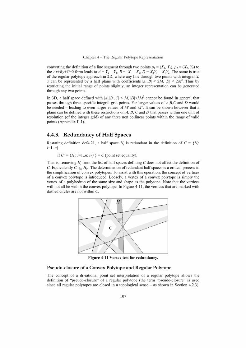
Chapter 4 – The Regular Polytope Representation
107
converting the definition of a line segment through two points p1 = (X1, Y1), p2 = (X2, Y2) to the Ax+By+C=0 form leads to A = Y2 – Y1, B = X1 – X2, D = X2Y1 – X1Y2. The same is true of the regular polytope approach in 2D, where any line through two points with integral X, Y can be represented by a half plane with coefficients |A|,|B| < 2M, |D| < 2M2. Thus by restricting the initial range of points slightly, an integer representation can be generated through any two points.
In 3D, a half space defined with |A|,|B|,|C| < M, |D|<3M2 cannot be found in general that passes through three specific integral grid points. Far larger values of A,B,C and D would be needed – leading to even larger values of M' and M''. It can be shown however that a plane can be defined with these restrictions on A, B, C and D that passes within one unit of resolution (of the integer grid) of any three non collinear points within the range of valid points (Appendix II.1).
4.4.3. Redundancy of Half Spaces Restating definition def4.21, a half space Hj is redundant in the definition of C = {Hi: i=1..n}
if C’ = {Hi: i=1..n: i≠j } = C (point set equality).
That is, removing Hj from the list of half spaces defining C does not affect the definition of C. Equivalently C’ ⊆ Hj. The determination of redundant half spaces is a critical process in the simplification of convex polytopes. To assist with this operation, the concept of vertices of a convex polytope is introduced. Loosely, a vertex of a convex polytope is simply the vertex of a polyhedron of the same size and shape as the polytope. Note that the vertices will not all be within the convex polytope. In Figure 4-11, the vertices that are marked with dashed circles are not within C.
C
H
Figure 4-11 Vertex test for redundancy.
Pseudo-closure of a Convex Polytope and Regular Polytope
The concept of a dr-rational point set interpretation of a regular polytope allows the definition of “pseudo-closure” of a regular polytope (the term “pseudo-closure” is used since all regular polytopes are closed in a topological sense – as shown in Section 4.2.3).
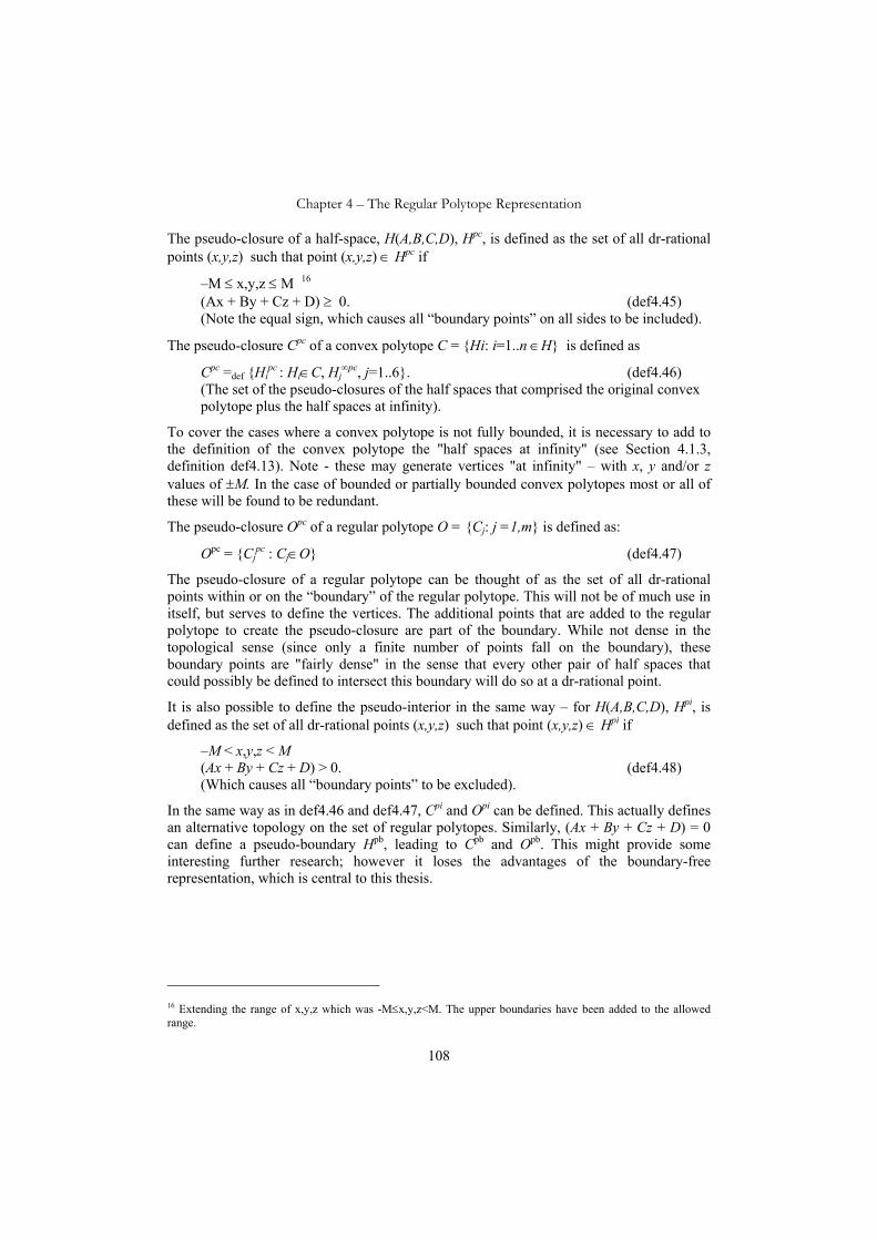
Chapter 4 – The Regular Polytope Representation
108
The pseudo-closure of a half-space, H(A,B,C,D), Hpc, is defined as the set of all dr-rational points (x,y,z) such that point (x,y,z) ∈ Hpc if
–M ≤ x,y,z ≤ M 16 (Ax + By + Cz + D) ≥ 0. (def4.45) (Note the equal sign, which causes all “boundary points” on all sides to be included).
The pseudo-closure Cpc of a convex polytope C = {Hi: i=1..n ∈H} is defined as
Cpc =def {Hipc : Hi∈C, Hj
∞pc, j=1..6}. (def4.46) (The set of the pseudo-closures of the half spaces that comprised the original convex polytope plus the half spaces at infinity).
To cover the cases where a convex polytope is not fully bounded, it is necessary to add to the definition of the convex polytope the "half spaces at infinity" (see Section 4.1.3, definition def4.13). Note - these may generate vertices "at infinity" – with x, y and/or z values of ±M. In the case of bounded or partially bounded convex polytopes most or all of these will be found to be redundant.
The pseudo-closure Opc of a regular polytope O = {Cj: j =1,m} is defined as:
Opc = {Cjpc : Cj∈O} (def4.47)
The pseudo-closure of a regular polytope can be thought of as the set of all dr-rational points within or on the “boundary” of the regular polytope. This will not be of much use in itself, but serves to define the vertices. The additional points that are added to the regular polytope to create the pseudo-closure are part of the boundary. While not dense in the topological sense (since only a finite number of points fall on the boundary), these boundary points are "fairly dense" in the sense that every other pair of half spaces that could possibly be defined to intersect this boundary will do so at a dr-rational point.
It is also possible to define the pseudo-interior in the same way – for H(A,B,C,D), Hpi, is defined as the set of all dr-rational points (x,y,z) such that point (x,y,z) ∈ Hpi if
–M < x,y,z < M (Ax + By + Cz + D) > 0. (def4.48) (Which causes all “boundary points” to be excluded).
In the same way as in def4.46 and def4.47, Cpi and Opi can be defined. This actually defines an alternative topology on the set of regular polytopes. Similarly, (Ax + By + Cz + D) = 0 can define a pseudo-boundary Hpb, leading to Cpb and Opb. This might provide some interesting further research; however it loses the advantages of the boundary-free representation, which is central to this thesis.
16 Extending the range of x,y,z which was -M≤x,y,z<M. The upper boundaries have been added to the allowed range.

Chapter 4 – The Regular Polytope Representation
109
Vertices of a Convex Polytope
The useful concept of a vertex can be defined as follows:
A vertex is a pseudo-rational point v = (x,y,z) ∈ Cpc which is within the pseudo-closure of the convex polytope, and there exist Hi, Hj, Hk ∈ C i≠j≠k≠i such that:
Aix + Biy + Ciz + Di = 0 (f4.34) Ajx + Bjy + Cjz + D j = 0 Akx + Bky + Ckz + Dk = 0
It is clear that this is just the normal definition of vertex in the classical convex solid polyhedron. (Note – in 2D, the vertices each need to be on exactly two half planes).
C
Figure 4-12 Convex polytope C with vertices circled.
Figure 4-12 should be interpreted as a 3D convex polytope sliced through the plane of one of its half spaces. Thus the circled vertices are the points of intersection of three half spaces. The intersections which are not circled are still the intersection of three half spaces, but are not within Cpc.
H1 H2
C
H3
Figure 4-13 Convex polytope C with vertices circled. New half spaces H1, H2 and H3
are to be added to the definition of C.

Chapter 4 – The Regular Polytope Representation
110
It is a useful property of these vertices that if a half space, which is being added to the definition of a convex polytope (such as H1(A1,B1,C1,D1) in Figure 4-13) is such that all vertices v = (x,y,z) of the convex polytope satisfy the inequality A1x+B1y+C1z+D1 ≥ 0, then H1 is redundant with respect to C, and need not be added. Similarly if for all vertices A2x+B2y+C2z+D2 ≤ 0, then H2 is incompatible with C (and if H2 is added to the set C, the result will be an empty convex polytope). Note that H3 is redundant to the definition of C although it passes exactly through a vertex.
All vertices must lie on grid2. That is to say, if p = (x,y,z) is a vertex, with x = Ix/Jx, y = Iy/Jy, z = Iz/Jz then |Ix|, |Iy|,|Iz|<N”, and |Jx|, |Jy|, |Jz| < N’, with N’ and N” as defined in f4.30 and f4.31.
Vertex Test for Redundant Half Spaces
If all existing vertices of a convex polytope are within the pseudo-closure of a half space, then the half space is redundant to the definition of the convex polytope. That is, all points within the convex polytope fall within the half space. (See Appendix IV.1 for the proof of this assertion).
Vertex Test for Incompatible Half Spaces
If all vertices of a convex polytope are within the pseudo-closure of the inverse of a half space, then the half space is incompatible with the convex polytope. That is there is no point within the convex polytope which is within the half space. (See Appendix IV.2 for proof).
4.4.4. Empty Test for a Convex Polytope The vertex test for incompatible half spaces allows a definition of the “Empty()” test for convex polytopes. A convex polytope C = {Hi: i=1..n} is empty if it has no vertices. That is to say, that for any point p = (x, y, z) that is the point of intersection of any three half spaces of C (including the half spaces at infinity if necessary) there exists Hj = H(Aj, Bj, Cj, Dj) such that Ajx+Bjy+Cjz+D < 0.
In practice, it is not necessary to apply this test explicitly. As a convex polytope is constructed, half spaces are added to it one by one. As half space H(A, B, C, D) is added, it can be compared with the vertices of the convex polytope as it existed before the addition. If all vertices v = (xk, yk, zk) are such that Axk+Byk+Czk+D ≥ 0 then H is redundant and need not be added. If all vertices are such that Axk+Byk+Czk+D ≤ 0 then H is incompatible with the existing half spaces, and the convex polytope becomes empty.
As described in Section 4.2.5, this allows a rigorous definition of the overlap, part of and the equals predicates, and the additional predicates of proper part, proper overlap and discrete from, in terms of dr-rational points of grid2.

Chapter 4 – The Regular Polytope Representation
111
4.4.5. Uniqueness of Convex Polytope Representation The justification of the approach is that, even though the definitions are framed in terms of dr-rational points, they can be shown to apply to all rational points regardless of precision. Thus it can be shown that for well defined half spaces:
H ≅ H’ ⇔ ∃ p ∈ Q Q 3
: (p ∈ H ⇔ p ∈ H’). (f4.35) where H ≅ H’ is as defined in def4.3: H(A, B, C, D) ≅ H’(A’, B’, C’, D’) =def ∃ integers I > 0, J > 0: AI = A’J, BI = B’J, CI = C’J, DI = D’J.
A well defined half space is defined as one which contains at least one dr-rational point.
It can also be shown (Appendix IV.4) that the definition of a convex polytope is unique, in that if two convex polytopes define the same rational point set, and all redundant half spaces are omitted, the resultant convex polytopes will be defined by the same number of half spaces, which are pairwise equal.
4.5. Floating Point Number Approach There is no theoretical reason that an approach based on the floating point number representation (either of A, B, C and D, or of the point coordinate values) could not be developed. Note, however, that it is not achievable by assuming that floating point is equivalent to real number arithmetic. Since the definitions of the algebra is in terms of point sets, it is vital that inclusion or exclusion of points in a set can be rigorously determined. Thus, if an algorithm can be developed for the rigorous determination of point set membership, a floating point approach would be possible. Note that this interpretation does not lead to a metric space as described in Section 4.2.2.
The definition and exploration of such an approach is outside the scope of this thesis.
4.6. Conclusion The concept of the regular polytope has been defined and its basic properties explored. The space spanned by regular polytopes has been shown to be a topological space, a metric space (apart from the floating point interpretation), and a Boolean algebra. The integer and dr-rational interpretations have been discussed in some detail, and a rigorous test for equality has been made available, along with a set of basic topological operations and predicates. It has been noted that there are clear advantages associated with the dr-rational interpretation of the regular polytope definition.
The next chapter will consider the important issue of connectivity between regions in relation to the regular polytope representation.


Chapter 5
Connectivity in the Regular Polytope Representation
The previous chapter defined the concept of a regular polytope and the basic topological functions and predicates between regular polytopes. The regular polytopes were shown to span a metric and topological space, and a Boolean algebra. The integer and dr-rational interpretations were defined, and discussed in some detail.
This chapter explores the important concepts of internal contiguity of regular polytopes, and connectivity between regular polytopes. Again, the integer and dr-rational forms are addressed, with the advantage of the latter being more strongly reinforced.
The concept and meaning of connectivity in general is discussed in Section 5.1, with a particular reference to connectivity of spatial regions as defined in geographic data models. In seeking a useful definition, it is found that a single definition is not sufficient to all requirements, so the two most useful (to be known as weak or Ca and strong or Cb connectivity) are defined and discussed in detail.
In Section 5.2 these definitions are applied to the convex polytope representation of spatial regions, using the integer and the dr-rational interpretations as presented in Chapter 4. It is shown that the Ca definition can be implemented using integer or dr-rational form, but that Cb is only completely satisfactorily supported by the dr-rational interpretation. These definitions are extended to the regular polytope in Section 5.3. Section 5.4 discusses the properties of the connectivity predicates as applied in this way, and Section 5.5 extends connectivity and overlap to a rich set of additional predicates. Section 5.6 introduces the issue of forming a partition of space into multiple regions using the regular polytope

Chapter 5 – Connectivity in the Regular Polytope Representation
114
approach. This issue will be discussed again in Chapter 8 from an implementation standpoint. Section 5.7 discusses the robustness of the regular polytope representation with regard to small perturbations in the definition of the half spaces.
5.1. Connectivity of Geometric Objects One of the more important properties of geometric objects is that of connectivity. Loosely, this can be thought of as the property that a geometric object has if it is “in one piece”; see Figure 5-1. It is the aim of this research to formalise this definition for regular polytopes in order to support robust determination.
In the polygon representation, as defined by standards such as ISO 19107 (ISO-TC211 2001), the connectivity of a polygon is mandated by requiring one (or zero) outer boundary, with zero or more inner boundaries. This does require further qualification to cover the cases of tangential connectivity. The regions in Figure 5-2 are not considered continuous by the ISO 19107 definition, because their interiors are not connected, but they are each defined using a single outer boundary. Egenhofer et al (1994) discuss the type of geometry, where parts of the boundary of a hole may be collinear with parts of the outer boundary (Figure 5-2 left region), and do consider it to be connected.
Figure 5-1 Examples of Connected Polygons.
A fuller discussion can be found in van Oosterom et al. (2004) with the following condition recommended for a valid polygon: “… any point inside or on the boundary of the polygon can be reached through the interior of the polygon from any other point inside or on the boundary of the polygon, that is, it defines one connected area”. The polygon on the right in Figure 5-1 is connected, but this definition eliminates the more problematic examples in Figure 5-2 and Figure 5-4. Frequently, where more than one outer boundary can exist, the geometry is known as a “multi-polygon” (OGC 1999b).
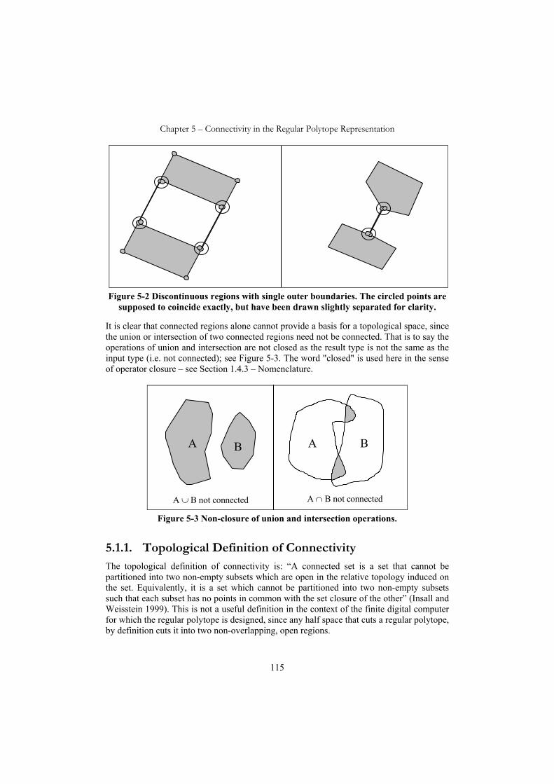
Chapter 5 – Connectivity in the Regular Polytope Representation
115
Figure 5-2 Discontinuous regions with single outer boundaries. The circled points are
supposed to coincide exactly, but have been drawn slightly separated for clarity.
It is clear that connected regions alone cannot provide a basis for a topological space, since the union or intersection of two connected regions need not be connected. That is to say the operations of union and intersection are not closed as the result type is not the same as the input type (i.e. not connected); see Figure 5-3. The word "closed" is used here in the sense of operator closure – see Section 1.4.3 – Nomenclature.
A ∪ B not connected A ∩ B not connected
A A BB
Figure 5-3 Non-closure of union and intersection operations.
5.1.1. Topological Definition of Connectivity The topological definition of connectivity is: “A connected set is a set that cannot be partitioned into two non-empty subsets which are open in the relative topology induced on the set. Equivalently, it is a set which cannot be partitioned into two non-empty subsets such that each subset has no points in common with the set closure of the other” (Insall and Weisstein 1999). This is not a useful definition in the context of the finite digital computer for which the regular polytope is designed, since any half space that cuts a regular polytope, by definition cuts it into two non-overlapping, open regions.

Chapter 5 – Connectivity in the Regular Polytope Representation
116
5.1.2. Alternative Definitions of Connectivity In order to provide a rigorous and useful definition of connectivity in the realm of regular polytopes, it is important first to decide what we wish to mean by “connected”. It is suggested1 that regions such as those pictured in Figure 5-2 should not be considered to be connected, but note that these regions contain a mixture of 1D and 2D parts and are therefore not regular in the topological sense (see Section 5.1.3). A more difficult issue is whether shapes such as those in Figure 5-4 should be considered to be internally connected, that is where the region of contact is not the same dimensionality as the regions themselves.
Figure 5-4 Marginal ‘connectivity’.
Cohn and Varzi (Cohn and Varzi 1999) identify twelve varieties of connection, based on two criteria (see also Section 3.2.6). The first criterion is determined by whether it is the interiors of the regions, the closures of the regions, or the regions themselves which connect. This is not an issue with the regular polytope representation, since a regular polytope has no boundary points. Thus only the second criterion need be considered. This is represented as Ca, Cb, Cc and Cd in Figure 5-5.
y
x
y
Ca
y
x
y
x x
y x
Cb Cc
CdOV
Figure 5-5 Connection relations Ca to Cd (Cohn and Varzi 1999), with overlap (OV)
depicted (based on Figure 3-3).
1 Following the OGC Simple Feature Specification usage.

Chapter 5 – Connectivity in the Regular Polytope Representation
117
Weak Connection
Ca Cb ⇒ Ca
OV ⇒ Cb ⇒ Ca
Strong Connection Overlap
0D meet 1D meet 2D meet 3D overlap
1 2 3 4 5 6
Figure 5-6 Modes of Connectivity in 3D (based on Figure 3-4).
Alternatively, connectivity may be described in terms of the dimensionality of the region of contact (Clementini et al. 1993), as discussed in Section 3.2.7. The interrelation of these approaches in shown in Figure 5-6.
The regions used in Figure 5-5 to illustrate Ca to Cd do not themselves overlap, (i.e. in the Cc and Cd cases, y has a hole the exact size of x). The definitions can be expressed loosely in 3D as:
• Ca if the regions touch (at one or more points, lines or surfaces – in Figure 5-6, the regions marked 1 and 2 meet at a point, 3 and 4 meet at a line).
• Cb if the regions touch at a surface in 3D or a line in 2D (in Figure 5-6, the regions marked Cb meet at a surface).
• Cc if the regions touch at the entire boundary of one region (in this case x completely fills a hole in y). (The inner and outer boundaries of y may touch).
• Cd if one region completely surrounds the other (x completely fills a hole in y and the inner and outer boundaries of y do not touch).
• OV if one region completely or partially overlaps the other (in Figure 5-6, the regions marked OV have volume in common).
The Cc and Cd varieties of connection are clearly too strong for most practical uses. These would normally be characterized by the word “enclosure” rather than “connection”. The Cb form of connection is clearly useful; it is the mode Ca which is more problematic. Borgo et al (1996) use the concept of “strong connection” (effectively Cb) to restrict the definition to what is intuitively a “physical connection” rather than mere contact. The analogy used is that a worm should be able to pass from one region to the other without exposing itself to the outside world. This is the form suggested by van Oosterom et al. (2004).
Commercial GIS and spatial DBMS products, ISO 19107 (ISO-TC211 2001) and the OGC Simple Feature Specification (OGC 1999b) are at considerable variance in their approaches to this question, and indeed, are often internally inconsistent (e.g. allowing contact between points on inner rings but not outer boundaries) (van Oosterom et al. 2004). Ultimately, the decision as to what variety of connectivity should be supported should be based on the “usefulness” of the result, with both being appropriate in different contexts. However

Chapter 5 – Connectivity in the Regular Polytope Representation
118
awareness of the issue and the existence of rigorous definitions helps to avoid some of the current interoperability issues.
In Chapter 6, the nomenclature of the region connection calculus (RCC) (Randell et al. 1992) is used to underpin the development of the algebra of the space of regular polytopes. For consistency with the RCC, Ca and Cb are taken to be implied by overlap. The definitions are not mutually exclusive. Thus:
Ca if the regions touch (at least at one point) or overlap. Cb if the regions touch at a surface (line in 2D) or overlap. Therefore: OV ⇒ Cb ⇒ Ca.
Arguments for Weak Connectivity - Ca
In the Cadastral information domain, connectivity of type Ca is argued for on the basis that any change in the definition of a parcel will affect all neighbours, including the “corner” neighbours.
A
D
B
C
p
E Road
q
F
Figure 5-7 Cadastral Parcels. A resurvey of parcel A could affect parcels C and F as
well as B, D and E.
The fact that a parcel is defined by a point which also is part of the definition of another parcel, could be taken as reason to assert that the parcels are connected. In Figure 5-7, the point p participates in the definition of parcels A, B, C and D, therefore its re-definition by a resurvey will affect all these parcels.
Difficulties with Ca
Although counter-intuitive, it is possible for two Ca connected regions to cross each other without their interiors intersecting (see Figure 5-8). This seems to be an undesirable property.

Chapter 5 – Connectivity in the Regular Polytope Representation
119
Figure 5-8 Two Ca connected regions crossing without intersecting.
Returning to Figure 5-7, a lot consisting of the amalgamation of parcels A and C would be Ca connected, as would the amalgamation of B and D, and these two lots would cross without overlapping.
Summary of Conclusions on Weak Connectivity
In summary, Ca is most likely to be useful when dealing with the connectivity between multiple regions, while Cb is more suitable for defining the internal connectivity of regions. It is apparent that both forms are useful and should be supported, and an awareness of the distinction is important in certain applications. The dimension of contact approach makes a finer distinction which could be important in certain problem domains.
5.1.3. Connectivity as Applied to the Regular Polytope In order to remove arbitrary distinctions between regions, based on concepts that have no real-world importance, [“… it is nonsense to ask whether a physical object occupies an open or a closed region of space, or who owns the mathematical line along a property frontier” (Lemon and Pratt 1998) page 10)], Lemon & Pratt invoke the concept of a regular set – see Section 1.4.4. A regular set is equal to the interior of its closure. In particular, the interior of the closure of any set is a regular set (possibly empty). Note that this interior may be disconnected.
The process of forming a regular region in this way removes some kinds of pathological connection such as those in Figure 5-2 (observe the result of these two cases in Figure 5-9). However this operation (‘make regular’) does not simplify the issue of point wise tangentiality as in the right polygon in Figure 5-1 and the polygons in Figure 5-4.

Chapter 5 – Connectivity in the Regular Polytope Representation
120
Figure 5-9 The shapes from Figure 5-2 and Figure 5-4 regularised.
The real issue with regular polytopes is whether a rigorous definition of connectivity can be formed.
5.1.4. Half Space Connectivity Issues In defining connectivity in the context of the regular polytope, it is essential that if a connected region is bisected by a half space (and its complement), then the two regions so created are connected to one another.
H H
O∩H
O∩H
Figure 5-10 A regular polytope bisected by a half space and its complement.
If O is a regular polytope, and it is divided by a half space H, then:
If HOOh ∩= , and HOOh ∩= , )()( HOHOOO hh ∩∪∩=∪
)( HHO ∪∩= = O (by the definition of complement of a half space)

Chapter 5 – Connectivity in the Regular Polytope Representation
121
Thus any definition of connectivity must require that )(C)(C hh OOO ∪⇔ . Note that by the definition of a half space and its complement there are no points common to both. This means, for example, that it is possible for two regular polytopes to be connected while having no points in common.
5.2. Connectivity of Convex Polytopes Before considering the question of connectivity between or within regular polytopes, it is useful to consider the question of connectivity between convex polytopes. As in Chapter 4, this will be considered in relation to the integer and the dr-rational number interpretations. The floating point interpretation is outside the scope of this thesis. In both cases, the issues of Ca and Cb continuity will be considered (but not Cc or Cd which are considered less useful in practice).
5.2.1. Connectivity in the Integer Interpretation Using the integer representation2 as introduced in Section 4.3, a definition of connectivity can be developed in terms of the minimum distance between points of the sets. For example: convex polytope A is Ca connected to B if there exists a point a∈A and a point b∈B, such that the distance between a and b is less than some defined constant ε. By this definition, it is obvious that OV ⇒ Ca.
Connected regions (minimum dist = 1 unit)
Disconnected regions (minimum dist > 2 units)
Figure 5-11 Inconsistent results for Ca with ε = 2 .
As can be seen in Figure 5-11, the choice of ε is important, but not obvious. A small value such as 1 or 2 (in terms of the grid1 unit size) can lead to a non-robust definition – in Figure 5-11, the case on the right is only a slight variation on that on the left, but the
2 Or in fact, using any other gridded representation. This approach could also be used for the dr-rational representation, but as will be seen below, better definitions are possible.

Chapter 5 – Connectivity in the Regular Polytope Representation
122
minimum distance has changed from 1 to 5 . On the other hand, a larger value of ε is likely to lead to spurious detection of contact in the case of near objects which do not touch.
One approach to defining Cb is to extend each convex polytope by a buffer the width of the grid interval, form the intersection of these extended convex polytopes, and count the grid points in the region of intersection of each convex polytope with the buffered version of the other.
To approximately buffer a convex polytope, it is simply necessary to decrease the value of Di in the definition of each half space Hi=H(Ai,Bi,Ci,Di). Replace the convex polytope
iniHC
..1== I by a larger one defined as '
..1' i
niHC
== I , where ),,,( ''
iiiii DCBAHH = and
( )iiiii CBADD ,,max' −= . This in effect, moves each half space one grid interval out from the convex region. This is clearly a convex polytope, and so the region of intersection is a convex polytope. It has been shown that it is possible to count the grid points in a convex region in polynomial time (Dyer 1991) in 3D (or 4D, or in any fixed number of dimensions by Barvinok (Barvinok 1994) ). This form of approximate buffering extends the convex polytope by one unit parallel to the x, y or z axis – depending on which of A, B or C has the largest absolute value. It is not possible to use buffering with a constant width (normal to the half space) as this requires D to be decreased by a multiple of
222 CBA ++ , which is not possible in general for integral D.
B
C
A’ B’
C’
A
D D’
Figure 5-12 Overlap of buffered convex polytopes.
It could be decided, for example, that if the number of points in the intersections of the buffered regions is less than (say) 26 (eight in 2D), then Ca is indicated. If the number is 26 or more, then Cb is indicated. The number 26 could be chosen because an overlap such as between A’ and B’ in Figure 5-12 (but in 3D) can cover up to that number of points, while still being clearly Ca. In the case of overlap, if p is the point in common between the two convex regions, then it is possible that not all of its 26 neighbouring points will be in the buffered overlap, so that it is necessary to include the requirement that OV ⇒ Cb as part of the definition. There are other clear deficiencies in this test. It is possible for two regions

Chapter 5 – Connectivity in the Regular Polytope Representation
123
such as B and D to be detected as Cb when in fact they really only nearly meet along a sufficiently long line (and should be only Ca).
Using the above definition, Cb cannot be guaranteed to support the following axiom, which is required by some of the algebras to be discussed in Sections 6.4 and 6.5:
(B4) ∀ X ≠ OΦ,Y ≠ OΦ,Z ≠ OΦ: C(X,Y∪Z) ⇔ [C(X,Y) ∨ C(X,Z)].
That is, if a region is connected to the union of two regions, it must be connected to at least one of them and vice versa. This axiom is included in the definition of a Boolean connection algebra (Section 3.2.4). An equivalent axiom (PS2) is used in the definition of a proximity space (Section 3.2.9).
Figure 5-13 illustrates a case where this axiom for Cb can break down. It is clear that Ca does satisfy this axiom, since the single point in the union that is adjacent to the other region must belong to at least one region.
B C
A
Figure 5-13 Breakdown of Axiom B4 (or PS2) in the integer interpretation of Cb.
An alternate approach to defining Cb in the integer interpretation is to determine if one or more half spaces from each convex polytope are separating them.
For C1 = {Hi: i=1..n1}, C2 = {Hj: j=1..n2}, if OV(C1, C2) or
∃ Hi ∈ C1, Hj ∈ C2: ji HH ≅ such that: letting C1’ = C1 – {Hi}, C2’ = C2 – {Hj} and C’ = C1’ ∪ C2’ C’ ∩ C1 ≠ CΦ, C’ ∩ C2 ≠ CΦ. Then Cb(C1, C2).

Chapter 5 – Connectivity in the Regular Polytope Representation
124
C1’
C2’ H9
C1
C2
C’
H1 H2
H3
H4
H5
H6
H7
H8
Figure 5-14 Alternative definition of Cb for the integer interpretation.
For example, in Figure 5-14, H3 and H9 are removed from C1 and C2 respectively (H9 is the complement of H3). The remaining half spaces then make the intersection C’ = {H1, H2, H4, H5, H6, H7} (H2 and H8 are redundant in the definition of C’). In this case, C’ ∩ C1 ≠ CΦ and C’ ∩ C2 ≠ CΦ, so that Cb(C1, C2).
This definition has some advantages over the other, in that it more directly models what is meant by Cb. On the other hand, it is dependent on the representation of the convex polytopes rather than their point set definitions. It is possible to generate a case where A = B as point set equality, but Cb(A, D) and ¬Cb(B, D).
H1
D
A
H2
H3
D’ A’
H1
H2 H3 D
B
B’
Figure 5-15 Although A in left figure equals B on right,
Cb(A, D) (left) but not Cb(B, D) (right).
For example, in Figure 5-15, 21 HH ≅ , and as point sets, A = B, but the overlap region in the left diagram intersects both A (in the region circled as A’) and D (in the region circled as D’). In the figure on the right, the overlap region does not intersect D. This in turn means

Chapter 5 – Connectivity in the Regular Polytope Representation
125
that the axiom B4 cannot be guaranteed to be satisfied. These are serious flaws in the definition, but do not prevent its use.
Thus we have at least two possible definitions for Cb in the integer interpretation, neither of which is entirely satisfactory.
5.2.2. Summary of Integer Interpretation Issues These definitions, for Ca and Cb, in conjunction with the definitions of union, intersection and inverse, allows the relations of the RCC to be implemented as is described in Chapter 6, however the algorithms for determining whether a convex polytope is equal to CΦ and the determination of Ca and Cb are complex. In addition, there is no clear qualitative difference between the situation between regions B and C in Figure 5-13 (which test as Ca but really should be Cb), and between the regions B and C in Figure 5-12 (which are clearly Cb). Similarly there is no qualitative difference in Figure 5-15 between A and D on the left, and B and D on the right. For these reasons, and because of the inherent lack of robustness of the integer based approach, the following dr-rational number based approach has been investigated.
5.2.3. Dr-Rational Definition of Ca Many of the difficulties with the integer interpretation can be relieved by using the dr-rational approach defined in Section 4.4. In that discussion it was noted that the algorithm to determine overlap was far simpler than in the integer approach. In a similar way, the approach simplifies the determination of connectivity.
Pseudo-closure of a Convex Polytope.
The concept of a dr-rational point set interpretation of a regular polytope allows the definition of “pseudo-closure” of a convex polytope (see Section 4.4.3). The pseudo-closure of a convex polytope can be thought of as the set of all dr-rational points within or on the “boundary” of the convex polytope. As was described in Section 4.1.3, a convex polytope contains all dr-rational points on its western edges, southern edges and bottom edges. This adds all points that also lie on the eastern and other edges.
p p
p
C1 C1 C1 C2 C2 C2
Figure 5-16 Examples of Ca connection that is not Cb or overlap.
Two convex polytopes C1 and C2 are considered to be Ca connected if there exists a dr-rational point p such that p is within C1
pc and within C2pc:

Chapter 5 – Connectivity in the Regular Polytope Representation
126
Ca(C1, C2) =def ∃p: p ∈ C1pc ∨ p ∈ C2
pc. (def5.1)
This will be denoted as Ca(C1,C2). Figure 5-16 illustrates three cases where Ca applies, but not any stronger type of connection. In all cases, the point marked p is part of region C2, but not region C1. It is within the pseudo-closure of C1 in all cases. Clearly, if OV(C1,C2), then ∃ p ∈ C1∩C2. This p is clearly within C1
pc and within C2pc therefore OV(C1,C2) ⇒
Ca(C1,C2). Note that in the alternate topology generated by the pseudo-interior and pseudo-closure operations, as mentioned in Section 4.4.3, this is just the conventional topological definition of connection as stated in Section 5.1.1.
Dr-Rational Definition of Cb
By contrast, the definition of Cb does not use the pseudo-closure. Instead, an axiomatic definition is used:
Cb(C1, C2) =def ∃C: C ⊆ C1∪C2 ∧ C∩C1 ≠ CΦ ∧ C∩C2 ≠ CΦ. (def5.2)
Note that C1 and C2 do not need to overlap, but a convex polytope must fit within the union of C1 and C2 and must cross the boundary, as shown in Figure 5-17. The actual implementation of Cb takes a slightly different form from this definition, but can be shown to be equivalent.
C1
C2 C
Figure 5-17 Cb Connectivity - C lies within C1 ∪ C2, and overlaps C1 and C2.
If C1 and C2 overlap, i.e. C1∩C2 ≠ CΦ, then letting C = C1∩C2, it is clear that C ⊆ C1∪C2, C∩C1 ≠ CΦ and C∩C2 ≠ CΦ. Therefore OV ⇒ Cb.
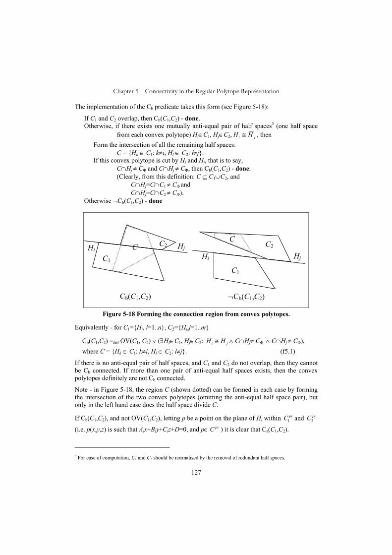
Chapter 5 – Connectivity in the Regular Polytope Representation
127
The implementation of the Cb predicate takes this form (see Figure 5-18):
If C1 and C2 overlap, then Cb(C1,C2) - done. Otherwise, if there exists one mutually anti-equal pair of half spaces3 (one half space
from each convex polytope) Hi∈C1, Hj∈C2, ji HH ≅ , then Form the intersection of all the remaining half spaces: C = {Hk ∈ C1: k≠i, Hl ∈ C2: l≠j}.
If this convex polytope is cut by Hi and Hj, that is to say, C∩Hj ≠ CΦ and C∩Hj ≠ CΦ, then Cb(C1,C2) - done.
(Clearly, from this definition: C ⊆ C1∪C2, and C∩Hj=C∩C1 ≠ CΦ and C∩Hj=C∩C2 ≠ CΦ). Otherwise ¬Cb(C1,C2) - done
C1
C2 C
C1
C2 C
Hi Hi
Hj Hj
Cb(C1,C2) ¬Cb(C1,C2)
Figure 5-18 Forming the connection region from convex polytopes.
Equivalently - for C1={Hi, i=1..n}, C2={Hj,j=1..m}
Cb(C1,C2) =def OV(C1, C2) ∨ (∃Hi∈C1, Hj∈C2: ji HH ≅ ∧ C∩Hj≠ CΦ ∧ C∩Hj ≠ CΦ), where C = {Hk ∈ C1: k≠i, Hl ∈ C2: l≠j}. (f5.1)
If there is no anti-equal pair of half spaces, and C1 and C2 do not overlap, then they cannot be Cb connected. If more than one pair of anti-equal half spaces exists, then the convex polytopes definitely are not Cb connected.
Note - in Figure 5-18, the region C (shown dotted) can be formed in each case by forming the intersection of the two convex polytopes (omitting the anti-equal half space pair), but only in the left hand case does the half space divide C.
If Cb(C1,C2), and not OV(C1,C2), letting p be a point on the plane of Hi within pcC1 and pcC2
(i.e. p(x,y,z) is such that Aix+Biy+Ciz+D=0, and p∈ pcC ) it is clear that Ca(C1,C2).
3 For ease of computation, C1 and C2 should be normalised by the removal of redundant half spaces.

Chapter 5 – Connectivity in the Regular Polytope Representation
128
Thus OV ⇒ Cb⇒ Ca. (f5.2)
For convenience, the empty convex polytope CΦ as defined as not being connected to any convex polytope. i.e. Ca(CΦ,C) = false and Cb(CΦ,C) = false. This will be further discussed in Chapter 6.
Using the dr-rational interpretation, it is clear that Ca and Cb connectivity support the axiom:
(B4) ∀ X ≠ OΦ, Y ≠ OΦ, Z ≠ OΦ: C(X,Y∪Z) ⇔ [C(X,Y) ∨ C(X,Z)].
Although this resembles the second definition of Cb in the integer interpretation, as described in Section 5.2.1 it does not share its problems, because of the uniqueness of the convex polytope representation in the dr-rational interpretation, as shown in Appendix IV.4. It is also important to note that the details of the interpretation, particularly the use of dr-rational numbers, and pseudo-closure are in some sense “under the covers”. To the outside observer, the definition of half space, and therefore convex and regular polytopes is in terms of integers. It is only when connection or overlap is to be determined that dr-rational arithmetic is required.
5.3. Connectivity of Regular Polytopes In either the integer or the dr-rational interpretations, two regular polytopes O1 and O2 are considered to be Ca or Cb connected if there exists a pair of convex polytopes C1 ∈ O1, C2 ∈ O2, such that Ca(C1,C2) or Cb(C1,C2). Note that this does not require that O1 or O2 are internally connected. In Figure 5-19, regular polytopes A (hashed) and B (shaded) are Cb connected to each other, but B is not internally connected.
A
B
B
B
Figure 5-19 Regular polytope connectivity.
For convenience, as with convex polytopes, the empty regular polytope OΦ is defined as not being connected to any regular polytope. i.e. Ca(OΦ,O) = false and Cb(OΦ,O) = false. This will be further discussed in Chapter 6.

Chapter 5 – Connectivity in the Regular Polytope Representation
129
5.3.1. Internal Connectivity of Regular Polytopes A regular polytope can be defined as “internally Ca connected” by induction as follows:
A Ca connection S within convex polytope O = {Ci: i=1..n} is defined as a set of convex polytopes S ={Ci: i=1..m: Ci∈O} such that:
S is a Ca connection if m =1. S’ ={Ck, Ci: i=1..m} is a Ca connection if {Ci, i=1..m} is a Ca connection, Ck∈O and ∃ i ≤ m such that Ca(Ck, Ci).
Figure 5-20 shows a regular polytope of 7 convex polytopes. These are grouped into three Ca connections.
A regular polytope iniCO
..1== U is Ca connected if {Ci, i=1..n} is a Ca connection.
1
2
3
2 b
2 a
Figure 5-20 Regular polytope containing three Ca connections.
Internal Cb connectivity can be defined in the same way for regular polytopes. Note that the regular polytope in Figure 5-20 has four parts which are Cb connections, marked 1, 2a, 2b and 3. Note that 2a and 2b are separate Cb connections because under the Cb criteria they are separated (¬Cb). Under the Ca criteria they are connected, and therefore belong to the same Ca connection.
5.4. Properties of CA and CB It is clear that in both the integer and the dr-rational interpretations the axioms required for a region connection calculus apply:
(Cref) Ca(O1,O1) and (Csym) Ca(O1,O2) ⇒ Ca(O2,O1),
and that the same apply to Cb. These axioms are basic to the RCC theory (Bennett 1995), which will be discussed in Chapter 6.

Chapter 5 – Connectivity in the Regular Polytope Representation
130
It is also clear from the similar results for convex polytopes that for the integer interpretation (see Appendix III for further details):
OV(O1, O2) ⇒ Cb(O1, O2), (f5.3) Cb(O1, O2) ⇒ Ca(O1,O2), (f5.4) ∀ O≠OΦ, O≠O∞, Ca ),( OO , ∀ X,Y,Z∈O: Ca(X,Y∪Z) ⇔ [Ca(X,Y) or Ca(X,Z)]. (f5.5)
For the dr-rational interpretation (see Appendix IV):
OV(O1, O2) ⇒ Cb(O1, O2), (f5.6) Cb(O1, O2) ⇒ Ca(O1,O2), (f5.7) ∀ O≠OΦ, O≠O∞, Ca ),( OO , (f5.8)
∀ O≠OΦ, O≠O∞, Cb ),( OO , ∀ X,Y,Z∈O: Ca(X,Y∪Z) ⇔ [Ca(X,Y) or Ca(X,Z)], (f5.9) ∀ X,Y,Z∈O: Cb(X,Y∪Z) ⇔ [Cb(X,Y) or Cb(X,Z)]. (f5.10)
5.5. Further Connectivity Relations Just as in Chapter 4, where P (part of), PP, (proper part of), PO (proper overlap), EQ (equal), and DR (discrete from) were defined in terms of the OV (overlap) relation, in this chapter we can define:
DCa (fully disconnected from) as: DCa(O1, O2) =def ¬Ca(O1, O2) (def5.3) ECa (externally weakly connected) as ECa(O1, O2) =def Ca(O1, O2) and ¬OV(O1, O2) (def5.4) TPPa (weakly tangential proper part) as TPPa(O1, O2) =def PP(O1, O2) and Ca(O1, 2O ) (def5.5) NTPPa (non-tangential proper part) as NTPPa(O1, O2) =def PP(O1, O2) and ¬Ca(O1, 2O ) (def5.6) DCb (partially disconnected from) as DCb(O1, O2) =def ¬Cb(O1, O2) (def5.7) ECb (externally strongly connected) as ECb(O1, O2) =def Cb(O1, O2) and ¬OV(O1, O2) (def5.8) TPPb (strongly tangential proper part) as TPPb(O1, O2) =def PP(O1, O2) and Cb(O1, 2O ) (def5.9) NTPPb (not strongly tangential4 proper part) as NTPPb(O1, O2) =def PP(O1, O2) and ¬Cb(O1, 2O ) (def5.10)
4 Names such as this can be confusing, so that the terminology “non-tangential B proper part” will be used in this thesis.

Chapter 5 – Connectivity in the Regular Polytope Representation
131
DCa DCb
ECa DCb
ECa ECb
NTPPa NTPPb
TPPa NTPPb
TPPa TPPb
Figure 5-21 Further connectivity relations based on weak and strong connectivity.
5.6. Partitioning of Space Many applications require that a complete non-overlapping coverage of the region of interest be maintained. For example, a cadastral database in 2D may require that the area of the jurisdiction be divided into land parcels, such that any point in the region can be said to fall within a single parcel, and can only belong to more than one if it falls on the boundary between two or more parcels. Using the regular polytope approach, this can be tightened to the requirement that every point in the region of interest falls within one and only one parcel. That is we wish to divide the domain of interest OR into regular polytopes Oi: i = 1..c such that:
i ≠ j ⇒ Oi ∩ Oj = OΦ, (f5.11) Ri
ciOO =
= ..1U . (f5.12)
It is possible to create such a coverage of regular polytopes, and ensure its completeness by virtue of the fact that the algebra is rigorous. Thus if we begin with a database consisting of one parcel only, being the OR, the domain of interest and add regular polytopes representing parcels to it using the following algorithm, a complete, non-overlapping coverage results.
Let P be the set of parcels in the database (where each parcel is a regular polytope). For every parcel O to be added to P:
Ensure that O ⊆ OR. Subtract O from each parcel already in P (i.e. for Oi∈P, replace Oi with Oi-O). Finally, add O to P.
This is similar to the algorithm used in the cellular model to insert feature shapes into a space partition (Bidarra et al. 1998).

Chapter 5 – Connectivity in the Regular Polytope Representation
132
D C E
F G
H I
J K
B A
p
Figure 5-22 Building a coverage.
This is by no means a complete answer to the issue of building a complete coverage in practice. As is illustrated in Figure 5-22, where it is assumed that the parcels have been entered in alphabetic order of their label, collisions and slivers can occur between parcels which might be intended to be adjacent. For example, inaccuracies in the placement of parcel D have resulted in a gap between it and parcel C. Points in this gap will remain part of the remainder parcel (shown shaded). This same inaccuracy has resulted in the eastern edge of D being shaved off by parcel E. Corners of parcels may be lost – as in the case of parcel F (shown exaggerated), and the point of common contact between a number of parcels can create a hiatus such as is shown at point p. It is presumed that p should represent a single point, but here, the overlap of the parcels has created a complex set of nearby points. There is also the question of the efficiency (or more correctly the speed of operation) of such an algorithm. These issues will be addressed in Chapters 7 and 8 as part of the discussion of the practicality of the regular polytope representation.
5.7. Robustness of Regular Polytopes As is the case for all representations of spatial data, it is important to know whether the representation is robust. That is to say “Is it sensitive to small inaccuracies of measurement and changes due to re-calculation of parameters?” It is assumed here that the resolution of the base units (grid1) is small compared with the true accuracy of the data (see Section 1.5.5 for discussion of integer and fixed-point representations). This is in common with all spatial data representations, where the resolution of storage and accuracy of calculations should be finer than the actual accuracy of the data to avoid degrading the data.
In this section, only the dr-rational interpretation is considered. Note that perturbations of the kind being considered here cannot cause a regular polytope to become invalid (as in the case of narrow cadastral parcels - Case 6 Section 2.6). What could occur is that a regular polytope could become disconnected, or a convex or regular polytope could become empty. In essence, this section looks at the question of topological changes occurring as a result of small perturbations – much smaller than the accuracy of the data.

Chapter 5 – Connectivity in the Regular Polytope Representation
133
5.7.1. Perturbation of a Half Space It is instructive to discuss the effect of small variations in the values of A, B, C and D in the definition of the half spaces that define a regular polytope.
For half space H = H(A, B, C, D), assume without loss of generality that |B| ≥ |A| and |B| ≥ |C|. If this is not the case, replace B with A or C in the following discussion, depending on which has the largest absolute value. (And replace x with y or z respectively).
If B = 0, then A = C = 0, then H = HΦ or H = H∞, and any change in the value of D does not change the meaning unless D changes sign, or becomes zero.
If B ≠ 0, consider H’ = (A+δ, B, C, D) for integer δ. If p = (x,y,z) is a dr-rational point on the defining plane of H, then consider p’ = (x,y’,z) on the defining plane of H’.
Ax + By + Cz + D = 0 (A+δ)x + By’ + Cz + D = 0 (A+δ)x - Ax + By’ - By = 0
Δy = y’ - y = xBδ
− (f5.13)
Thus the displacement of the plane caused by a perturbation of δ in the value of A is no greater than x
Bδ
− .
Similarly, replacing C with C+δ gives Δy = y’ - y = zBδ
− (f5.14)
Consider H’ = (A, B+δ, C, D), with p’ = (x,y’,z) on the defining plane of H’.
Ax + By + Cz + D = 0 Ax + (B+δ)y’ + Cz + D = 0 (B+δ)y’ - By = 0
y’ = yB
Bδ+
y’ - y = yB
BBδδ)(
++−
Δy = y’ - y = yB δδ+
− (f5.15)
Consider H’ = (A, B, C, D+δ), with p’ = (x,y’,z) on the defining plane of H’.
Ax + By + Cz + D = 0 Ax + By’ + Cz + (D+δ) = 0 By’ – By + δ = 0
Δy = y’ - y = Bδ
− (f5.16)
Note that the displacement of the plane caused by variations of A, B and C increases for points further from the origin. Note also that the larger the values of |A|, |B|, |C| and |D| are,

Chapter 5 – Connectivity in the Regular Polytope Representation
134
the less sensitive the final result is to perturbation. Also note that it is always possible to ensure that max(|A|,|B|,|C|) > ½M, because it is always possible to multiply all of the coefficient values by a positive constant without changing the half space.
For large M, and max(|A|,|B|,|C|) > ½M, the greatest displacement of the plane of H by varying A, B, C, and D each by a maximum of δ occurs at a point with x, y, or z = ±M which, substituting f5.13 to f5.16 above gives
displacement < 22212
δδδδMMMM MMM +++
+ ≈ 6δ. (f5.17)
Note that even though this result is derived for dr-rational points, it also carries over to the integer interpretation, but the movement of the plane may not be a whole number of grid intervals.
5.7.2. Robustness of Convex Polytopes It is of interest whether the perturbation of the half spaces that define a convex polytope C can cause it to become empty. Assume the half spaces are perturbed so that the maximum movement of the surface of any half space within the range of the convex polytope is δ. This can be formalised as saying that if any point p ∈ C is at least δ units from all half spaces then p will be guaranteed to be within the perturbed convex polytope.
C H v1
v2
δ
Figure 5-23 A regular polytope which is not robust with respect to perturbation of
more than δ units.
For example, in Figure 5-23, the half space H is less than 2δ units from vertices v1 and v2 (the dashed lines indicate a buffer of δ units inside and outside H). Thus there can be no point p which is more than δ units within all half planes within C. If all half planes are moved by δ units in the worst direction, this convex polytope could become empty. Note, in Figure 5-23 the dotted lines showing the limit of perturbation of H should not be interpreted as indicating that only parallel movement of H is possible. What is being considered is any movement of H that does not cause it to move by more than δ units in the neighbourhood of the regular polytope.
For a convex polytope, as a quick test for robustness in 2D, if the area A of the enclosed region divided by its perimeter P is greater than δ, the convex polytope is robust. In 3D, if

Chapter 5 – Connectivity in the Regular Polytope Representation
135
the volume V divided by the surface area S is greater than δ, the convex polytope is robust. This test is pessimistic, and in 2D it is possible for a convex polytope to have A/P of δ/2 and still be robust. Likewise, in 3D V/S of δ/3 could be robust. Some cases are illustrated in Figure 5-24, remembering that if δ < h/2, the convex polytope is robust. Note that it is relatively easy using conventional geometric formulae to calculate the volume and surface area of a 3D convex polytope, as it is to calculate the area and perimeter of a 2D convex polytope.
h
h
h h
A = ½Bh, P ≈ 2B h ≈ 4A/P
A = Bh, P ≈ 2B h ≈ 2A/P
V = Ah/3, S ≈ 2A h ≈ 6V/S
V = Ah, S ≈ 2A h ≈ 2V/S
Figure 5-24 Limiting cases of robust convex polytopes in 2D and 3D.
5.7.3. Robustness of Ca Connected Convex Polytopes If two convex polytopes are Ca connected, but not Cb, then they must meet at a single vertex or at an edge between two vertices. This means that they are not robustly connected, since perturbation in the wrong direction of any of the half planes defining the point or edge of contact will break the connectivity. Thus two Ca connected convex polytopes are robustly connected only if they are robustly Cb connected.
It could be argued that a robust Ca connection is possible, since any anti-equal pair of half spaces is unlikely to be generated accidentally. Thus for example, in Figure 5-25, the polytope on the left has two pairs of anti-equal half spaces, 52 HH ≅ and 63 HH ≅ . The polytope on the right has no anti-equal pairs. A case could be made for a robustness criterion to consider that anti-equal pairs of half spaces are perturbed as a unit – leading to the polytope on the left being considered to be robustly connected. Section 7.3 discusses a particular data model which supports this definition of robustness.

Chapter 5 – Connectivity in the Regular Polytope Representation
136
H1
H2
H3 H4
H5
H6 H7
H8
H1
H2
H3 H4 H5
H6
H7
H8
Figure 5-25 Robust and fragile Ca connectivity.
5.7.4. Robustness of Cb Connected Convex Polytopes As described in Section 5.2.3, the test for Cb connectivity between two convex polytopes C1 and C2 is in two parts – they may overlap or have a pair of half spaces in common.
Overlapping Convex Polytopes
In the case of overlap, the convex polytope of overlap is calculated C = C1 ∩ C2. If this convex polytope C is robust in respect to perturbations of up to δ, then the Cb connectivity can be taken as robust up to a displacement of δ. Note that a convex polytope must itself be robust if it is to overlap another robustly.
Non-Overlapping Convex Polytopes
If Cb(C1, C2) and not OV(C1, C2), then there exist H1 ∈ C1 and H2 ∈ C2 such that H1 ≅ 2H and if C’1 is C1 – {H1}, and C’2 is C2 – {H2}, and C’ = C’1∩ C’2, then by the definition of Cb connectivity:
C”1 = C’ ∩ C1 ≠ CΦ, and C”2 = C’ ∩ C2 ≠ CΦ.
The connectivity can be called robust (at measure δ) if C”1 is robust at measure δ, and C”2 is robust at measure δ. Again, note that a convex polytope must itself be robust if it is to be robustly connected to another. This is based on the assumption that any anti-equal pair of half spaces are intended to be anti-equal and do not become separated. The data model described in Section 7.3 supports this concept.
Thus we can define a regular polytope to be internally connected at measure δ if the convex polytopes that comprise it are pathwise robustly connected at measure δ. If Cδ is taken to mean “robustly connected at measure δ”, it is clear that:
Cδ(C1, C2) ⇒ Cb(C1, C2) ⇒ Ca(C1, C2).

Chapter 5 – Connectivity in the Regular Polytope Representation
137
5.8. Robustness of Connected Regular Polytopes In certain applications it may desirable to mandate that a feature must be connected, where such connectivity is an intrinsic attribute of the type of object being represented. We can define a robustly connected regular polytope at measure δ using an inductive definition as was used to define a Ca or Cb connected polytope in Section 5.3.1. A regular polytope can be defined as Cδ (robustly connected at measure δ) by induction as follows:
A Cδ connection S within convex polytope O = {Ci: i=1..n} is defined as a set of convex polytopes S ={Ci: i=1..j: Ci∈O} such that:
S is a Cδ connection if j=1 and Cj is robust at measure ≥ δ. S’ = {Ck, Ci: i=1..j} is a Cδ connection if S = {Ci, i=1..j} is a Cδ connection, Ck∈O and ∃ i ≤ j such that Cδ(Ck, Ci).
A regular polytope iniCO
..1== U is Cδ connected if {Ci, i=1..n} is a Cδ connection.
For example, in Figure 5-26, this regular polytope is robustly connected, in spite of the weak connection between convex polytopes A and E; because a strong connection is available via a path ABCDE. In this example, the limiting connection is between B and C, and if Cδ(B, C) then we can say the regular polytope is internally Cδ connected.
A
B C
D
E
Figure 5-26 Robust connection of a regular polytope composed of five convex
polytopes.
This discussion has assumed that the value of δ has been decided, and the connectivity is being tested against the chosen value, but this can be turned around as suggested in Case 4 Section 2.4 and in Thompson and van Oosterom (2006a), to define a robustness attribute ρ of O as the maximum value of δ for which there exists a path through all Ci ∈ O, with each connectivity being at measure δ or better. This is not a simple determination, since in the general case, it will require a “best path” traversal of the convex polytopes in order to

Chapter 5 – Connectivity in the Regular Polytope Representation
138
determine which possible path gives the largest value of ρ, but a well known algorithm is available.
5.9. Conclusions The definition of the regular polytope has been extended to include the question of connectivity and it has been shown that the weak (Ca) and strong (Cb) varieties can be supported rigorously. Using the integer based interpretation, the full capabilities of Ca can be realised, but there are some restrictions on the Cb form such as the failure of the Boolean connection algebra axiom B4 (see Section 6.4).
By contrast, the dr-rational interpretation of the regular polytope supports a fully rigorous implementation of Ca and Cb. It has further been shown that a rich set of functionality can be defined in terms of these and the topological operations described in Chapter 4. The issues of the robustness of the representation and robustness of connectivity have been explored.
The following chapter discusses in detail the formal algebras that can thus be supported, with emphasis on the region connection calculus, the Boolean connection algebra and the proximity space.

Chapter 6
Algebras of Connectivity
In the earlier chapters, a construct known as the regular polytope has been defined, and augmented by a set of topological and connectivity operations and predicates which have been shown to be implementable using integer or fixed precision rational arithmetic. It has further been shown that using the integer based interpretation, the full capabilities of weak (Ca) connectivity can be realised, but there are some restrictions on the strong (Cb) form. By contrast, the dr-rational interpretation of the regular polytope supports a fully rigorous implementation of strong and weak connectivity.
This chapter discusses the formal algebras that can thus be supported, and investigates the expressivity of the regular polytope approach, comparing its functionality against, for example:
the region-connection calculus (Randell et al. 1992), the proximity space (Naimpally and Warrack 1970), Boolean connection algebra (Düntsch and Winter 2004).
Use is also made of the "Egenhofer 9 matrix" (Egenhofer 1994) in these discussions for comparison purposes. The regular polytope representation is evaluated in its ability to support a range of topological and geometric functions, and to support imprecise relationships and fuzzy logic.
Section 6.1 reviews the region connection calculus (briefly introduced in Section 3.2.8) in comparison with related work. Section 6.2 uses the framework of the RCC operations and predicates to formalise the logic of the regular polytope, while an alternate approach – involving the dimensionality of contact is considered briefly in Section 6.3. The relationship with the proximity space (Section 3.2.9) and the Boolean connection algebra
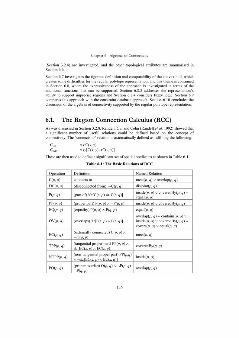
Chapter 6 - Algebras of Connectivity
140
(Section 3.2.4) are investigated, and the other topological attributes are summarised in Section 6.6.
Section 6.7 investigates the rigorous definition and computability of the convex hull, which creates some difficulties for the regular polytope representation, and this theme is continued in Section 6.8, where the expressiveness of the approach is investigated in terms of the additional functions that can be supported. Section 6.8.3 addresses the representation’s ability to support imprecise regions and Section 6.8.4 considers fuzzy logic. Section 6.9 compares this approach with the constraint database approach. Section 6.10 concludes the discussion of the algebras of connectivity supported by the regular polytope representation.
6.1. The Region Connection Calculus (RCC) As was discussed in Section 3.2.8, Randell, Cui and Cohn (Randell et al. 1992) showed that a significant number of useful relations could be defined based on the concept of connectivity. The "connects to" relation is axiomatically defined as fulfilling the following:
Cref ∀x C(x, x) Csym ∀xy[C(x, y)→C(y, x)].
These are then used to define a significant set of spatial predicates as shown in Table 6-1.
Table 6-1: The Basic Relations of RCC
Operation Definition Named Relation C(p, q) connects to meet(p, q) ∨ overlap(p, q) DC(p, q) (disconnected from) ¬C(p, q) disjoint(p, q)
P(p, q) (part of) ∀z[C(z, p) ⇒ C(z, q)] inside(p, q) ∨ coveredBy(p, q) ∨ equal(p, q)
PP(p, q) (proper part) P(p, q) ∧ ¬P(q, p) inside(p, q) ∨ coveredBy(p, q) EQ(p, q) (equality) P(p, q) ∧ P(q, p) equal(p, q)
OV(p, q) (overlaps) ∃z[P(z, p) ∧ P(z, q)] overlap(p, q) ∨ contains(p, q) ∨ inside(p, q) ∨ coveredBy(p, q) ∨ covers(p, q) ∨ equal(p, q)
EC(p, q) (externally connected) C(p, q) ∧ ¬O(q, p) meet(p, q)
TPP(p, q) (tangential proper part) PP(p, q) ∧ ∃z[EC(z, p) ∧ EC(z, q)] coveredBy(p, q)
NTPP(p, q) (non-tangential proper part) PP(p,q) ∧ ¬∃z[EC(z, p) ∧ EC(z, q)] inside(p, q)
PO(p, q) (proper overlap) O(p, q) ∧ ¬P(p, q) ¬P(q, p)
overlap(p, q)

Chapter 6 - Algebras of Connectivity
141
At first sight, this may seem to be a small number of relations compared to the 512 that can be identified using the Egenhofer 9 matrix (Egenhofer 1994), but as has been shown by Egenhofer and Franzosa (1995) only eight of them are distinct and applicable to pairs of contiguous surfaces in 2D, or pairs of contiguous solids in 3D (see Table 6-2). These have been named, and are more basic than the RCC relations in that they are disjunct and complete (exactly one relation is true for any pair of operands). For example, the "meet" relationship means meet without overlap, while the "connects to" relation means meet or overlap. The relationship between the named relations and the RCC relations is also shown in Table 6-1.
Table 6-2: The Named Relations
Named Relation
Matrix and Sketch RCC Equivalent
disjoint 0 0 10 0 11 1 1
A B
DC(A,B)
contains 1 1 10 0 10 0 1
A B
NTPP(B,A)
inside 1 0 01 0 01 1 1
B A
NTPP(A,B)
equal 1 0 00 1 00 0 1
A B
EQ(A,B)
meet 0 0 10 1 11 1 1
A B
EC(A,B)
covers 1 1 10 1 10 0 1
A B
TPP(B,A)
coveredBy 1 0 01 1 01 1 1
B A
TPP(A,B)
overlap 1 1 11 1 11 1 1
A B
PO(A,B)

Chapter 6 - Algebras of Connectivity
142
The asymmetric relations inside(p, q) and coveredBy(p, q) are equivalent to the other pair of relations contains(q, p) and covers(q, p) respectively. Note the difference between the RCC "overlaps" from the "overlap". Thus all of the discrete relations between connected, bounded regions of the same dimensionality can be represented by the RCC algebra. The predicates C, P, PP and OV are composite relationships.
Based on a spherical universe (Egenhofer 2005), an additional three relations are possible (Figure 6-1).
attach entwined embrace
Figure 6-1 The additional three topological relations realised in a spherical space, adapted from Egenhofer (2005).
The 512 relations have been further analysed, to determine which are possible given regions of different dimensionality (2000; Zlatanova et al. 2002), however if regions are permitted to be unbounded, omitting Zlatanova's condition C1 (“The exteriors of two objects always intersect”), there are additional relations that are expressible in the Egenhofer matrix beyond those named above. These are shown for regions of the same dimensionality in Table 6-3, where the outer rectangle is used to represent the universal region (and the heavier shading represents the region of overlap of A and B). In the RCC, they are recognized simply as EC, and O. In the regular polytope algebra, the complement predicate could be defined as ),(EQ BA , unbounded overlap covering space as ),(PP AB . The other unbounded overlap predicates are not particularly useful.

Chapter 6 - Algebras of Connectivity
143
Table 6-3 Additional Relationships where Regions may be Unbounded
1 1 1 1 0 1 1 0 1
1 1 1 1 0 1 1 1 1
entwined 1 1 1 1 1 1 1 0 1
unbounded overlap covering space
1 1 1 1 0 0 1 0 0
B A
1 1 1 1 1 0 1 1 1
unbounded overlap
1 1 1 1 0 0 1 1 1
A B
0 0 1 0 1 0 1 0 0
B A
B A
B A
A
A
B
B
B A
entwined
unbounded overlap
unbounded overlap
complement
entwined covering space
1 1 1 1 1 0 1 0 0
The convergence between the functionality of the Egenhofer relations and the RCC relations is particularly significant, because it must be remembered that the former are defined in terms of the boundaries, while the RCC does not build on the concept of a boundary. That is to say, the concepts of adjacency, contact and overlap can be fully developed in a mereological sense (see Section 3.2.11), without assuming the existence of infinite boundary sets.
6.1.1. Region Connection Calculus in a Finite Space As discussed in Section 3.2.8, a major complication is that the sequence of definitions as given in Randell et al (1992), is not compatible with a finite topological space. The original (RCC) approach was to define the “part of” relation P(X, Y) (also represented as X ⊆ Y) in terms of the connection relation. The definition was:
P(X,Y) =def ∀Z[C(Z,X)→C(Z,Y)] (f6.1)
This definition had the unwanted and surprising side effect that it required the space to be non-atomic – that is, every region can be subdivided into smaller regions. The argument (Randell et al. 1992) can be summarised as follows: assume region A to be atomic (i.e. has no subset apart from the empty region OΦ). Let R be any other region R ≠ OΦ. If R ≠ A, then R is connected to A . If R = A, then R is connected to A . Thus
),(C),(C: ARARR ⇒∀ therefore AA ⊆ .

Chapter 6 - Algebras of Connectivity
144
The paper (Randell et al. 1992) discussed the possibility of an “atomic” RCC theory, defining a non-atomic ("proper") region as:
PROP_REGION(X) =def ∃Z:NTPP(Z,X) (f6.2)
However the argument by Düntsch et al (2002), shows that this definition is redundant, and that all regions in an RCC are proper. Roy and Stell (2002) discuss this in a context of a discrete space, and conclude that this approach cannot be maintained. The approach of Roy and Stell uses a dual pseudo-complement lattice (Balbes and Dwinger 1974) to deal with the boundary point sets, but this is unnecessary in the case of the regular polytope topology.
The definition of half space, which eliminates any boundary point sets, allows the simpler Boolean connection algebra to be used (Section 3.2.4), with the only variation being that the axiom B5, which ensures an infinitely smooth space, is omitted (see Section 3.2.4).
In the regular polytope approach, the “part-of” predicate P is not defined in terms of connectivity so that this pitfall is avoided. Instead, part-of is defined in terms of overlap. (See Section 4.2.5).
6.2. The Spatial Relations on Regular Polytopes The nomenclature of the relations between regular polytopes as used in this thesis follows those defined by Randell, Cui and Cohn (1992), however the semantics are slightly different. In particular, for reasons as discussed above (Section 6.1.1), the sequence of these definitions could not follow the order of definition they described. As a practical implementation strategy the following sequence is observed:
• The basic functions: intersection, union and negation on regular polytopes are defined first (Section 4.1).
• The isEmpty(P) test on regular polytopes is defined (Section 4.2.5). • These are used to define part of, overlap and equality (Section 4.2.5). • Connectivity is defined as Ca or Cb as required (Sections 5.3 and 5.3). • These are then combined to define the remaining RCC relations (Section 5.5).
Note that the RCC makes no distinction between weak and strong connectivity, and in fact does not assign any restriction on what can be called a connection relation apart from needing to satisfy the axioms. Therefore since both Ca and Cb satisfy Cref and Csym, the theory can be applied to either form.
6.2.1. The Empty and Universal Regular Polytopes As was noted in the preceding chapter, the approach taken here handles the empty regular polytope OΦ and the universal regular polytope O∞ as follows, leading to the consistent (but not necessarily obvious) results:
∀O, ¬Ca(OΦ, O); ∀O≠OΦ, Ca(O∞, O); (f6.3) ∀O, ¬Cb(OΦ, O); ∀O≠OΦ, Cb(O∞, O); (f6.4) ∀O, OΦ ⊆ O ⊆ O∞; (f6.5)
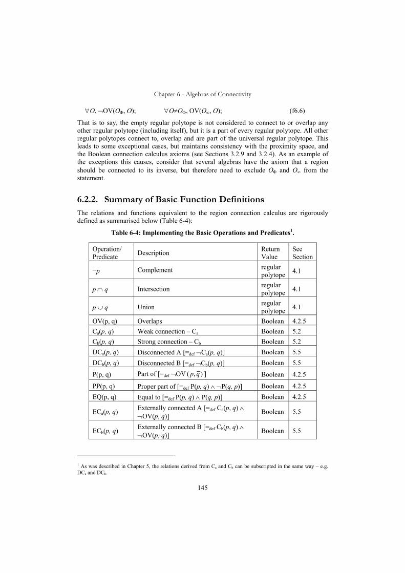
Chapter 6 - Algebras of Connectivity
145
∀O, ¬OV(OΦ, O); ∀O≠OΦ, OV(O∞, O); (f6.6)
That is to say, the empty regular polytope is not considered to connect to or overlap any other regular polytope (including itself), but it is a part of every regular polytope. All other regular polytopes connect to, overlap and are part of the universal regular polytope. This leads to some exceptional cases, but maintains consistency with the proximity space, and the Boolean connection calculus axioms (see Sections 3.2.9 and 3.2.4). As an example of the exceptions this causes, consider that several algebras have the axiom that a region should be connected to its inverse, but therefore need to exclude OΦ and O∞ from the statement.
6.2.2. Summary of Basic Function Definitions The relations and functions equivalent to the region connection calculus are rigorously defined as summarised below (Table 6-4):
Table 6-4: Implementing the Basic Operations and Predicates1.
Operation/ Predicate Description Return
Value See Section
¬p Complement regular polytope 4.1
p ∩ q Intersection regular polytope 4.1
p ∪ q Union regular polytope 4.1
OV(p, q) Overlaps Boolean 4.2.5 Ca(p, q) Weak connection – Ca Boolean 5.2 Cb(p, q) Strong connection – Cb Boolean 5.2 DCa(p, q) Disconnected A [=def ¬Ca(p, q)] Boolean 5.5 DCb(p, q) Disconnected B [=def ¬Cb(p, q)] Boolean 5.5
P(p, q) Part of [=def ¬OV ),( qp ] Boolean 4.2.5
PP(p, q) Proper part of [=def P(p, q) ∧ ¬P(q, p)] Boolean 4.2.5 EQ(p, q) Equal to [=def P(p, q) ∧ P(q, p)] Boolean 4.2.5
ECa(p, q) Externally connected A [=def Ca(p, q) ∧ ¬OV(p, q)]
Boolean 5.5
ECb(p, q) Externally connected B [=def Cb(p, q) ∧ ¬OV(p, q)] Boolean 5.5
1 As was described in Chapter 5, the relations derived from Ca and Cb can be subscripted in the same way – e.g. DCa and DCb.

Chapter 6 - Algebras of Connectivity
146
TPPa(p, q) Tangential proper part A [=def PP(p, q) ∧ Ca(p, q )] Boolean 5.5
TPPb(p, q) Tangential proper part B [=def PP(p, q) ∧ Cb(p, q )] Boolean 5.5
NTPPa(p, q) Non-tangential proper part A [=def PP(p, q) ∧ ¬Ca(p, q )] Boolean 5.5
NTPPb(p, q) Non-tangential proper part B [=def PP(p, q) ∧ ¬Cb(p, q )] Boolean 5.5
PO(p, q) Proper overlap [=def OV(p, q) ∧ ¬P(q, p) ∧ ¬P(p, q)] Boolean 4.2.5
DR(p, q) Discrete from [=def ¬OV(p, q)] Boolean 4.2.5
6.3. Dimensionality of Overlap An equivalent approach could have been used based on the dimensionality of the region of contact between the regular polytopes (Clementini et al. 1993). Following this approach, the predicates C0, C1, C2, C3, … can be defined, where the subscript is the dimensionality of the overlap. Thus C0(A, B) means that pseudo-closures of regular polytopes A and B meet at a 0D region – a point, C1 – at a line etc. In a 2D embedding space, therefore C0 is equivalent to (Ca ∧ ¬Cb) (strictly weak connection only), C1 ≡ (Cb ∧ ¬OV) and C2 ≡ OV (overlap) (see Figure 6-2). Thus in 2D, all the arguments for the rigorous logic based on Ca, Cb and OV can be applied, with the difference being nomenclature only.
C1 = Cb (1D meet)
C2 = OV (2D meet)
C0 = Ca (0D meet)
Figure 6-2 Dimensionality of overlap (in 2D).
In a 3D embedding space, C0 and C1 are different forms of weak connection – Ca, while C2 ≡ (Cb ∧ ¬OV) and C3 ≡ OV. Figure 6-3 (which is an extended version of Figure 3-4) shows the correspondence in 3D.

Chapter 6 - Algebras of Connectivity
147
Weak Connection
Ca
Cb ⇒ Ca
C3 = OV ⇒ Cb ⇒ Ca
Strong Connection Overlap
0D meet 1D meet 2D meet 3D meet
C0 C1 C2
Figure 6-3 Dimensionality of overlap (in 3D).
Thus, to provide a logic on this basis, it is necessary in 3D to distinguish between a point of contact, and a line of contact. Using the integer representation, this is problematic, but the dr-rational approach allows a clean definition. For the dr-rational representation of convex polytopes in 3D, C0 connectivity can be defined as C0(C1, C2) if there is at least one vertex of C1 within C2
pc, or vice versa. C1 connectivity can be defined as requiring exactly two vertices, however these could be two vertices from C1 within C2
pc, or vice versa, or one vertex from each within the other (not at the same location). The non-degeneracy of the convex polytope means that this cannot lead to any problematic special cases.
O1 O2
C0
O1 O2
C1
O1 O2
C2
O1 O2
C3
Figure 6-4 Dimensionality of overlap of regular polytopes.
The connectivity between two regular polytopes is defined as the maximum dimensionality of contact between any convex polytopes that comprise them (see Figure 6-4). By contrast, the internal connectivity of a regular polytope is defined as the weakest connection along a path between its component convex polytopes (see Section 5.3.1).
6.4. Proximity Space As described in Section 3.2.9, the axioms given for a proximity space X with the proximity relation δ, regions A, B, C, E ⊆ X and empty region ∅ are (Naimpally and Warrack 1970):
(PS1) A δ B ⇒ B δ A (PS2) (A ∪ B) δ C ⇔ A δ C ∨ B δ C

Chapter 6 - Algebras of Connectivity
148
(PS3) A δ B ⇒ A ≠ ∅ ∧ B ≠ ∅ (PS4) 2 A δ B ⇒ ∃ E: A δ E ∧ (X-E) δ B (PS5) A ∩ B ≠ ∅ ⇒ A δ B.
The axiom PS4 is known as the "strong axiom", and a proximity space which does not satisfy this axiom is known as a weak proximity space. In effect, this axiom requires a dense space, and so is not satisfied by the regular polytope space.
6.4.1. Integer Interpretation It can be shown (see Appendix III.4) that a weak proximity space can be generated by the integer interpretation using Ca. As was discussed in Section 5.2.1, using the integer representation, the Cb connectivity cannot be guaranteed to support PS2, which is equivalent to the Boolean connection algebra axiom B4.
6.4.2. Dr-Rational Number Interpretation It can also be shown (see Appendix IV.10) that the space of regular polytopes based in the dr-rational representation satisfies the axioms for a weak proximity space, using either the Ca or the Cb form of connectivity. This is a further reason for preference being given to the dr-rational approach.
6.5. Boolean Connection Algebra As was discussed in Section 4.2.4, with proof in Appendix II.11, the space of regular polytopes satisfies the axioms for a Boolean algebra. Roy and Stell (2002) also add axioms equivalent to the following to define connectivity, thus creating a Boolean connection algebra:
(B1) C(X, Y) ⇒ C(Y, X) (B2) C(X, X) for X ≠ OΦ (B3) ∀ ),(:),( XXCOOXX ∞Φ≠ (B4) ∀ X ≠ OΦ, Y ≠ OΦ, Z ≠ OΦ: C(X,Y∪Z) ⇔ [C(X,Y) ∨ C(X,Z)]. (B5) ∀ X ≠ O∞ , ∃ Y ≠ OΦ : ¬C(X,Y).
The final axiom requires that the space be continuous, since if X is atomic, there cannot be any region Y that is not connected to X. It is relatively easy to show that axioms B1 to B4 are satisfied by regular polytopes over the dr-rational interpretation, and using Ca or Cb (see Appendix IV.9), so that the space of regular polytopes could be considered as a discrete Boolean connection algebra (BCA). As was discussed above, using the integer
2 In this axiom, δ means “not δ”.

Chapter 6 - Algebras of Connectivity
149
interpretation, only Ca can be used to define a discrete BCA (Appendix III.3), since the axiom B4 cannot be guaranteed by Cb connectivity.
6.6. Properties of the Space of Regular Polytopes It has been shown above that the space of regular polytopes obeys the axioms for the region connection calculus, and that it forms a weak proximity space and a Boolean connection algebra3. It is important to remember that this is the computational representation that satisfies the axioms, not an abstraction which is approximated by the computational representation. Thus it is possible to computationally apply the operations in any combination with complete confidence that no logic failure can result. Some further properties of the space of regular polytopes follow, but first some terminology is included.
6.6.1. Disconnected Space “A space is connected if it cannot be split into two non-empty disjoint open sets” (Hurewicz and Wallman 1948 Page 10). Since any half space does this (H and H are both open sets), this implies that the space of all regular polytopes is not connected. That is, it has dimension = 0 in the topological sense. Note that the set of all rational numbers is 0D, and the set of all computer representable points is also 0D.
6.6.2. The Space of Regular Polytopes The space of regular polytopes has been shown to be metric, and therefore is T0 to T4 (see Sections 3.2.1 and 3.2.2). It is also disconnected, as mentioned above. Since any regular and connected space must be uncountable, the countability of the space of regular polytopes implies its disconnectedness. Thus the set of regular polytopes forms a finite, disconnected non Euclidean metric space (which is also therefore normal, regular, Hausdorff, etc.).
6.6.3. Atomicity of the Space A space is described as non-atomic if every region can be subdivided into smaller sub-regions. In terms of the RCC, a region is described as “proper” if it contains at least one non-tangential proper part (Randell et al. 1992). In an atomic space, there must exist regions – known as atoms, which cannot be further subdivided. Since the number of points that can be represented in any computer is finite (albeit very large), the space of regular polytopes cannot be non-atomic. This has already been discussed in Section 6.1.1 in the context of the region connection calculus.
3 Except that as described above, the integer representation cannot satisfy the latter two using Cb connectivity.

Chapter 6 - Algebras of Connectivity
150
6.7. The Convex Hull Randell, Cui and Cohn (1992) present a rigorous (axiomatic) definition of the concept of a convex hull, so it is reasonable to ask whether the regular polytope represents this definition correctly. Unfortunately, this definition is problematic for the regular polytope in the dr-rational or integer representation. The axioms given in Randell, Cui and Cohn for CONV(X), the convex hull of region X are:
CH1. ∀X: P(X, CONV(X)) (X is part of its convex hull) CH2. ∀X: P(CONV(CONV(X)), CONV(X)) 4 CH3. ∀X∀Y∀Z [[P(X, CONV(Y)) ∧ P(Y, CONV(Z))] → P(X, CONV(Z))] CH4. ∀X∀Y [[P(X, CONV(Y)) ∧ P(Y, CONV(X)) ] → OV(X, Y)] CH5. ∀X∀Y [[DR(X,CONV(Y)) ∧ DR(Y,CONV(X))] → DR(CONV(X), CONV(Y))]
The definition for a convex polytope is simple, but the problem is that a regular polytope with concavities will require one of more half planes to be used to “paper over” these concavities. To be exact and to satisfy these axioms exactly, these will need to meet the existing edges exactly.
p
q
r s
H
J
A
B
C
D
E
regular polytope
X F
Figure 6-5 Forming an exact convex hull.
For example, in Figure 6-5, to cover the concavity at faces C and D of regular polytope X, it is necessary to generate half spaces H and J which pass exactly through points p, q, r and p, s, q respectively. Unfortunately, as discussed in Section 3.4.6, since these are dr-rational points, the new half spaces require a significantly larger domain to store their parameters. Thus the resulting convex hull is therefore not a convex polytope (by definition). If two or more convex hulls are then used in union and/or intersection operations, a new geometry type will result, similar to a regular polytope, but requiring increased domain in the definition of its parameters. If an attempt is then made to form the convex hull of this new
4 Note, that this also implies that EQ(CONV(CONV(X)), CONV(X)), or more simply, CONV(CONV(X)) = CONV(X).
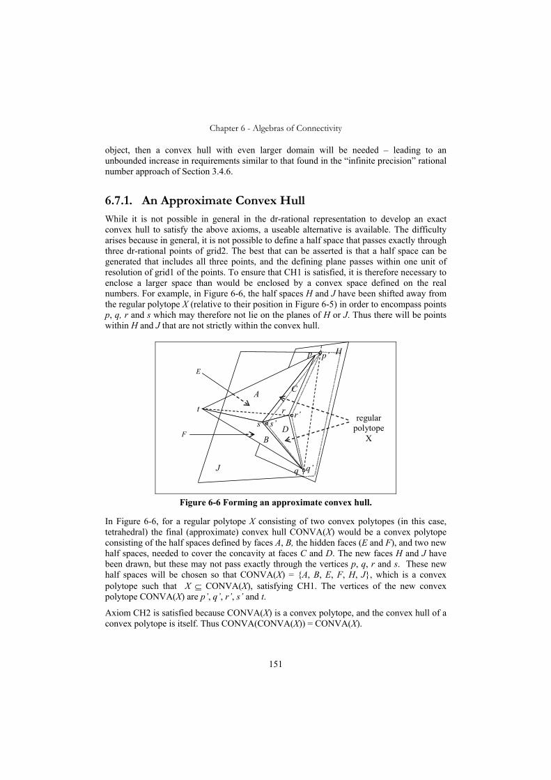
Chapter 6 - Algebras of Connectivity
151
object, then a convex hull with even larger domain will be needed – leading to an unbounded increase in requirements similar to that found in the “infinite precision” rational number approach of Section 3.4.6.
6.7.1. An Approximate Convex Hull While it is not possible in general in the dr-rational representation to develop an exact convex hull to satisfy the above axioms, a useable alternative is available. The difficulty arises because in general, it is not possible to define a half space that passes exactly through three dr-rational points of grid2. The best that can be asserted is that a half space can be generated that includes all three points, and the defining plane passes within one unit of resolution of grid1 of the points. To ensure that CH1 is satisfied, it is therefore necessary to enclose a larger space than would be enclosed by a convex space defined on the real numbers. For example, in Figure 6-6, the half spaces H and J have been shifted away from the regular polytope X (relative to their position in Figure 6-5) in order to encompass points p, q, r and s which may therefore not lie on the planes of H or J. Thus there will be points within H and J that are not strictly within the convex hull.
p
q
r s
H
J
A
B
C
D
E
p’
q’
s’ r’ regular
polytope X F
t
Figure 6-6 Forming an approximate convex hull.
In Figure 6-6, for a regular polytope X consisting of two convex polytopes (in this case, tetrahedral) the final (approximate) convex hull CONVA(X) would be a convex polytope consisting of the half spaces defined by faces A, B, the hidden faces (E and F), and two new half spaces, needed to cover the concavity at faces C and D. The new faces H and J have been drawn, but these may not pass exactly through the vertices p, q, r and s. These new half spaces will be chosen so that CONVA(X) = {A, B, E, F, H, J}, which is a convex polytope such that X ⊆ CONVA(X), satisfying CH1. The vertices of the new convex polytope CONVA(X) are p’, q’, r’, s’ and t.
Axiom CH2 is satisfied because CONVA(X) is a convex polytope, and the convex hull of a convex polytope is itself. Thus CONVA(CONVA(X)) = CONVA(X).

Chapter 6 - Algebras of Connectivity
152
The remaining three axioms cannot be satisfied in general. For a counter example to axiom CH3 see Figure 6-7. Here X is part of the convex hull of Y, and Y is part of the convex hull of Z, but X is not within the convex hull of Z. Note – these are drawn in 2D, but really represent a slice through 3D polytopes.
Z Y X
Figure 6-7 : P(X, CONVA(Y)) ∧ P(Y, CONVA(Z)) ∧ ¬ P(X, CONVA(Z)).
With axiom CH4, it is difficult to show a clear picture of a violation, and the axiom would follow in all reasonable cases, but if extremely thin regular polytopes are involved, it would be possible to construct a case such as in Figure 6-8, where X and Y do not overlap, but each is included within the convex hull of the other. In this case, both regions must be thinner than the grid size of the coarsest grid (less than one grid unit wide). (These are clearly not useful representations, and would not be robust as defined in Section 5.7. The case is only constructed to illustrate the breaking of the axioms.)
X
Y
Figure 6-8 Two non-overlapping regular polytopes each enclosed by the other's
convex hull.
For a counter-example of axiom CH5, see Figure 6-9. Here the two regions are discrete (not connected) from each other's convex hulls, but their convex hulls overlap.

Chapter 6 - Algebras of Connectivity
153
X
Y
CONVA(X) CONVA(Y)
Figure 6-9 : DR(X, CONVA(Y)) ∧ DR(Y, CONVA(X)) ∧ O(CONVA(X), CONVA(Y)).
Thus this approximation of the convex hull is not a true conforming definition. It is, however, a practical approximation which remains within one unit of resolution of the true convex hull. Thus, while it could be used for certain purposes, it cannot be relied on for rigorous logic operations.
6.7.2. The Convex Enclosure An alternative approach is to define a convex enclosure function of a regular polytope CONVE(O), which returns a convex polytope, and obeys axioms such as:
CE1. ∀O: O ⊆ CONVE(O) (O is part of its convex enclosure) CE2. ∀C (C is a convex polytope) CONVE(C) = C CE3. ∀O (O is a regular polytope), C' ⊂ CONVE(O) ⇒ ¬(O ⊆ C'), where C' is a convex polytope.
(For clarity, the proper part operation – PP(C’, C) is denoted C’ ⊂ C – see Section 6.1). This in effect would define a convex enclosure as the smallest convex polytope that encloses the regular polytope. This would be an acceptable replacement for the convex hull, and would be indistinguishable from it in any practical situation, but provides an axiomatic definition that could be used to extend the algebra in a rigorous fashion. It is not known at present if this can be implemented in practice, but it is clear that a unique convex enclosure exists for every regular polytope.
Assume C and C1 are convex polytopes which form enclosures of regular polytope O (i.e. O ⊆ C, O ⊆ C1). If any point p exists such that p ∈ C1, p ∉ C, then form the intersection C ∩ C1. Note that p ∉ O. Now C ∩ C1 is a proper subset of C which is also an enclosure of O. Replace C with C ∩ C1.
This procedure can be repeated for any other convex polytopes that enclose O. Since the number of possible convex polytopes that can be represented is finite, this procedure must terminate. Note that this is an existence proof, not necessarily a practical algorithm, since the number of half spaces so generated could be very large.
Assume that this procedure has been done twice, and C1 and C2 are the final products, and assume C1 ≠ C2. ∃ p: p ∈ C1, p ∉ C2 or p ∈ C2, p ∉ C1. In either case, p ∉ C1 ∩ C2 and p ∈ O. Thus C1 ∩ C2 ⊂ C1 or C1 ∩ C2 ⊂ C2 and O ⊆ C1 ∩ C2. This is a contradiction to the

Chapter 6 - Algebras of Connectivity
154
assumption that C1 and C2 were each end results of the process. Thus the convex enclosure of a regular polytope exists, and is unique. Note also that for any half space H, O ⊆ H ⇒ CONVE(O) ⊆ H.
Z Y
p
H
Figure 6-10 Axiom CH3 in the CONVE function.
Clearly, axioms CE1 and CE2 imply CH1 and CH2 respectively, but in addition, the convex enclosure also satisfies axiom CH3. Referring to Figure 6-10,
Let Y ⊆ CONVE(Z).
Assume ∃ p, p ∈ CONVE(Y), p ∉ CONVE(Z), then
∃ H (a half space): H ∈ CONVE(Z), p ∉ H. But Y ⊆ CONVE(Z) ⇒ Y ⊆ H. Therefore CONVE(Y) ⊆ H, (because CONVE is minimal) and so p ∉ CONVE(Y) - contradiction. So that X ⊆ CONVE(Y), Y ⊆ CONVE(Z) ⇒ X ⊆ CONVE(Z).
It seems likely that axioms CH4 and CH5 are not necessarily satisfied by CONVE, and there may not be any practical algorithm for its calculation. This could be considered as a subject for further research.
6.8. Expressiveness of the Relations and Functions Spatial relationships and in particular predicates to be used in searching data are fundamental to spatial databases. As such, a rich set must be provided by any system that purports to support spatial data storage and retrieval. On the other hand, there is no definitive set of such required functionality, merely a widely accepted set of functions that have been found useful. This section discusses some of the relations which have been or could be defined, and which may be useful in certain problem domains. There are two broad classes of spatial function to be considered here – the topological and the geometric.

Chapter 6 - Algebras of Connectivity
155
6.8.1. Topological Functions and Predicates The RCC relations are described in Section 6.2.2 above, and are all rigorously supported by the regular polytope approach. Other collections of topological relations, operations and predicates can be supported by the regular polytope representation as described below.
Topological Relationships Defined Using the Egenhofer Matrix
In addition to the RCC relations, there are some relationships that can be defined by the Egenhofer matrix, where the regions in question are not themselves internally connected (Egenhofer 1994) or are not bounded.
A
B B
Figure 6-11 Non RCC Relationship between regions.
For example, the relation ⎟⎟⎠
⎞⎜⎜⎝
⎛
111100111
can be satisfied by two regions A and B in Figure 6-11
where one part of region B overlaps region A. This is only possible because the region B is not internally connected, allowing the interiors of A and B to intersect without their boundaries meeting. This would simply be detected in the regular polytope space as OV(A,B), however an additional test such as "isConnected(A∪B)" could make the distinction if it is deemed important. There are many such relationships that can be posited, and in general, they cannot be distinguished by a single RCC predicate.
Topological Relationships not Discriminated by the Egenhofer 3 × 3 Matrix
There are some useful relations that cannot be discriminated by the Egenhofer 9 matrix, although they are covered in an extension to the theory (Egenhofer et al. 1994). These relations are also not discriminated by the RCC theory. For example, the regions in Figure
6-12 are just disconnected - DC(A,B), and the Egenhofer matrix is ⎟⎠
⎞⎜⎝
⎛111100100
, which is the
same as that of DC(A,B). The regular polytope representation would not detect this situation without specific coding.

Chapter 6 - Algebras of Connectivity
156
d i s c o n n e c t e d s u r r o u n d e d b y
A
B
A
B
Figure 6-12 "Surrounded by" and “disconnected” relationships.
In addition, the four forms of connectivity discussed in Section 3.2.6 after Cohn and Varzi (1999), cannot be distinguished by the Egenhofer 9 matrix. All of the relationships shown
in Figure 6-13 would be characterised by the matrix ⎟⎠
⎞⎜⎝
⎛111110100
. The regular polytope makes
no attempt to distinguish the Cc and Cd forms of connectivity. (In any case, they do not appear to be of much practical significance).
y
Ca
y
Cb
y
Cc
y
Cd x
x x
x
Figure 6-13 The connection relations Ca to Cd (see also Chapter 3).
6.8.2. Geometric Functions and Predicates
The RCC Spatial Relationships
As discussed in Section 6.2, the basic relations of the RCC are all supported by the regular polytope representation, apart from the convex hull. This is only handled as an approximation by the regular polytope approach. Thus the "Within Convex Hull" predicate is not available rigorously. This also implies that the GEO-INSIDE predicate defined in (Randell et al. 1992) can only be approximated. See Figure 6-14.
Measurement-Based Geometric Relationships
The distance function is most useful in practical situations, but cannot be provided as a mathematically exact number by any computer-based calculation. This is obvious from the
Chapter 6 - Algebras of Connectivity
157
fact that the square-root must be calculated in the process. The regular polytope clearly shares this restriction with all other systems, but provided it is remembered that the result is approximate, and not needed in further exact calculations, this is not seen as a restriction.
On the other hand, it is possible to determine buffered predicates (e.g. find all features within 1km of a feature) exactly and rigorously in the dr-rational representation, provided that additional precision of calculation is available. If it is necessary to determine whether two points are within distance r of one another, r2 can be calculated and compared with a measure defined as: for p1 = (x1,y1,z1), p2 = (x2,y2,z2):
212
212
212212 )()()(),( zzyyxxppd −+−+−= (def6.1)
So that, if p1 and p2 are such that d2(p1, p2) < r2, then the points are sufficiently close. It is fairly simple to extend this approach to convex polytopes, and therefore to regular polytopes.
Likewise, angular measures in general cannot be calculated exactly in terms of the bearing in degrees between two points, between the origin and a point, or between a line segment and an axis5. Again, an approximate measure can be calculated, as in conventional vertex-based representations and it is possible to define exact and rigorous directional predicates of a specific (restricted, but useful) type. Any half space defines a region, and can be used in the same way as a regular polytope in a predicate. For example, the predicate – “A is above 1000m” is equivalent to A ⊆ H, where H is the half space H(0,0,1,t) – with t being 1000m in the units of resolution. Many of the useful directional predicates can be expressed in this fashion as half spaces or combinations of them – e.g. “north of”, “south east of”, “above”. In addition, slopes defined in terms of their gradient (“gradient of 1 in 30”), (i.e. tan(s) where s is the slope angle) can be rigorously represented.
Other Geometric Relationships
There are many other geometric relationships that can be imagined, some of which are supported in currently available software, and some which are not. In Figure 6-14, some of these are illustrated simply to highlight that the conventially provided set of predicates is not definitive. GEO-INSIDE and TOPO-INSIDE (or “surrounded” – see Section 6.8.1) are discussed by Randell, Cui and Cohn, but the others are included just for discussion.
The TRAPPED predicate could possibly be useful, and is intended as indicating that region B cannot be moved through the gap in A. The OBSCURED predicate is one that could also potentially be useful in GIS applications, where the region B cannot be seen by an observer who is not GEO_INSIDE(A).
5 This is true of angles in 2D and in 3D.

Chapter 6 - Algebras of Connectivity
158
GEO-INSIDE TOPO-INSIDE TRAPPED OBSCURED
A A A
A
B B B B
Figure 6-14 Some other possible region predicates.
As discussed above, the GEO-INSIDE predicate is not rigorously definable using the convex hull axioms (see Section 6.7), but may be definable using the CONVE function. The remaining predicates may be rigorously definable, but this question is beyond the scope of this thesis.
6.8.3. Imprecise Relationships The convex polytope representation is well suited to the representation of imprecise regions. It must be remembered that the rigorous nature of the representation is needed to ensure internal reliability of the logic, and does not in any way suggest that the original data are highly accurate. The approaches to dealing with imprecision carry over directly from the conventional vertex representations, with some care.
It is possible to buffer any half space by simply adding to the D value of the half space definition – i.e. if H = H(A, B, C, D), then H’ = (A, B, C, D+δ), δ > 0 is a larger half space H ⊂ H’. An approximate buffer about d units wide can be generated around a convex polytope C = {Hi: i = 1..n}, where Hi = (Ai, Bi, Ci, Di) as:
C’ = {H’i: i = 1..n} where
H’i = ⎟⎠⎞⎜
⎝⎛ ⎟
⎠⎞⎜
⎝⎛ ++− 222NINT,,, iiiiiii CBAdDCBA . (def6.2)
It is assumed that the square root function, and its product with d can be calculated using floating point arithmetic, and that the NINT function returns the nearest integer to the result. If the floating point operations are done in 8 byte precision, the resultant buffer will be almost within ½ of a grid1 spacing from the true buffer width. The buffered region from a regular polytope is simply the union of the buffered convex polytope that comprises it. This is an approximate buffer only, but since the resultant object is a regular polytope, can be used rigorously in all calculations, and therefore all further operations are fully defined. There is a potential issue with acute corners, as can be seen around corner p in Figure 6-15, where the buffers around C1 and C2 extend beyond what would be thought of as the buffer around the regular polytope, and at corner q, where the new vertex is considerably further from q than the buffer width d.

Chapter 6 - Algebras of Connectivity
159
p
C1 C2
q
>d
Figure 6-15 Approximate buffering of a regular polytope.
A preferable approach is to use the measure defined in def6.1 which was: 2
122
122
12212 )()()(),( zzyyxxppd −+−+−= for p1 = (x1,y1,z1), p2 = (x2,y2,z2). (def6.3)
In this approach, a pair of regular polytopes O1, O2 can be determined as being within distance r of one another if there exist points p1 ∈ O1
pc, p2 ∈ O2 pc such that d2(p1, p2) ≤ r2.
Equivalently:
d2(O1, O2) = min[d2(p1, p2)]: p1 ∈ O1pc, p2 ∈ O2
pc. (def6.4)
Using the symbology of Section 3.2.13 as illustrated in Figure 6-16, for region R defined as a regular polytope, at an imprecision of δ, R4 can be defined as:
R4(R, δ) = {O: d2(O, R) ≤ δ2}. (def6.5)
O3∈R3
O4∈R4
O5∈R5
O1∈R1
O2∈R2
W
Figure 6-16 Imprecision in a region source (from Figure 3-6).
The negative buffer sets of regions R1 and R2 are not so easily defined. In the same way as the vertex representations, the negative buffer of an acute angled corner does not provide a good model of a negative buffer. For example, in Figure 6-17, if the buffer width represents the imprecision of measurement of the vertices, both regions A and B should be recognised as overlapping region C, no movement of the vertices of the order of the imprecision will

Chapter 6 - Algebras of Connectivity
160
cause the regions not to intersect. The negative buffers of each are disjoint from C, so they will be detected as uncertain overlap (R4 instead of R2 as described in Section 3.2.13). Note that in the case of region B no vertex lies within C. This is an issue that needs further research, and the regular polytope shares this difficulty with all other representations (see also Figure 3-7).
A B
C
Figure 6-17 Negative buffering difficulties.
6.8.4. Fuzzy Logic An alternate approach to limited precision of regions is the use of fuzzy logic, as discussed in Section 3.2.14. In relation to the current subject, this can be summarised as the replacement of the concept of hard edged sets with sets which have imprecise boundaries, defined by a characteristic function. A classical set A in Rn can be described as a function χA: Rn → {0, 1}. That is to say, each point in Rn is assigned the value 1 = true or 0 = false, indicating that the point is within A or not. (Dilo 2006). In the fuzzy logic approach, a real-valued function μ: Rn → [0, 1] is used. This is interpreted as point p is definitely within the set if μ(p) = 1, p is definitely outside if μ(p) = 0, and any other value of μ(p) indicates the degree of certainty of containment (with the larger value meaning more certain).
The first issue is that a real-valued function cannot be directly represented within a computer system, so that in the regular polytope representation, the function μ is replaced by a many valued function. This has no significant effect except where discontinuities occur in the function μ. At such points of discontinuity, the effect is the same as in the crisp logic, that a small change in position causes a discontinuous result.
It is useful in this context to compare the definition of a half space with the Hessian normal form (Weisstein 2002b) definition of a plane. In this form, real numbers a, b, c and d correspond to the integer coefficients A, B, C and D with (a, b, c) constituting a unit vector normal to the plane such that:
a = 222 CBA
A
++, b =
222 CBA
B
++, c =
222 CBA
C
++and
d = 222 CBA
D
++.

Chapter 6 - Algebras of Connectivity
161
The advantage of Hessian form is that the value of d is the distance from the origin to the nearest point on the plane of H. In addition, for any point p = (x,y,x), h = ax+by+cz+d is the distance between point p and the plane of H, with a positive value of h meaning the point is within the half space. By comparison, the distance between p = (x, y, z) and the plane of a half space H(A, B, C, D) is:
222 CBA
DCzByAxh++
+++= (f6.7)
Clearly, this can only be calculated approximately in a digital representation, for example as a floating point number, but this is acceptable in the fuzzy logic approach. A half space could be interpreted as “fuzzy” if the definition from Chapter 4 were replaced by:
μ(x, y, z) = 21
21
21
222,,maxmin +⎟⎟
⎠
⎞
⎜⎜
⎝
⎛⎟⎟⎠
⎞⎜⎜⎝
⎛−
++
+++
CBAr
DCzByAx (f6.8)
where r is a “fuzziness parameter”, a floating point number (a larger value of r means a less well defined boundary). This is illustrated in Figure 6-18, where the half space H is replaced by the function μ(x, y, z).
H
μ = 1
μ = 0 r
Cross section of μ(x,y,z) along the dashed line.
r
Hμ = 1
μ = 0
Figure 6-18 Fuzzy interpretation of a half space H.
An alternate form of the function μ could be:
μ(x, y, z) = duer
du
∫ ∞−
⎟⎠⎞
⎜⎝⎛ −
−2
21
21 σ
σπ (f6.9)
where r = 222 CBAr
DCzByAx
++
+++ (f6.10)
The rationale for this characteristic function is that it represents the probability that a point p would be within the half space H(A, B, C, D) if the position of the half space is inaccurately determined with a normal distribution with standard deviation of σ (Fraser 1958) (see Section 3.2.14). The shapes of these functions are shown (f6.8 and f6.9) in the 1D case in Figure 6-19. This figure could also be interpreted as a cross section of a 2D

Chapter 6 - Algebras of Connectivity
162
fuzzy half plane, or a 3D fuzzy half space. The difficulty in using this function is that it never reaches 0 or 1, and so cannot define regions such as those shown in Figure 6-16. That is to say, its transition zone extends to infinity.
d r
σ
f6.8
f6.9
transition zone
Figure 6-19 Characteristic functions of a fuzzy half line in 1D.
Other functions could be devised, some more appropriate, but the following will assume that the function being used has the following characteristics:
It is monotonic in terms of x, y and z. It is continuous at all points –M ≤ x, y, z < M.
These fuzzy half spaces can be combined to form “fuzzy convex polytopes” and “fuzzy regular polytopes” as described in chapter 4, and a form of fuzzy algebra could be defined. Each object has a characteristic function μ. For example, letting the function that corresponds to Hi = H(Ai, Bi, Ci, Di) be:
μ1(x, y, z) = 21
21
21
222,,maxmin +⎟⎟⎟
⎠
⎞
⎜⎜⎜
⎝
⎛
⎟⎟⎟
⎠
⎞
⎜⎜⎜
⎝
⎛−
++
+++
iii
iiii
CBAr
DzCyBxA (f6.11)
Then the defining function for the fuzzy convex polytope C = {Hi: i = 1..n} could be defined as:
μC(x, y, z) = ( )),,(μmin..1
zyxini= (f6.12)
Similarly the defining function for the fuzzy regular polytope R = {Cj: j = 1..m} could be defined as:
μR(x, y, z) = ( )),,(μmax..1
zyxjCmj=
(f6.12)
As a simple example, in Figure 6-20, a fuzzy convex polytope is formed in 2D from four fuzzy half spaces. The “side view” is intended to show how the value of μ varies from 1 within the region through intermediate values to 0 at the exterior of the region.

Chapter 6 - Algebras of Connectivity
163
μ = 1
μ = 0
top view side view
H1 H2
H2
H3
H4 H4
r
Figure 6-20 A "fuzzy convex polytope" in 2D.
However there is an important consideration in this definition. Consider a fuzzy half space as defined by either of the functions defined above. If H is a fuzzy half space defined by either function μ as defined in f6.8 or f6.9, considering this as a function of A, B, C and D, it can be readily verified that:
∀ x, y, z: μ(A, B, C, D) = 1 - μ(-A, -B, -C, -D). (f6.13)
Thus it can be seen that if μ(A, B, C, D) is a characteristic function for H, then μ(-A, -B, -C, -D) will provide a good characterisation of H , the inverse of H. This is suitable, and fits well with the definition of the (crisp) regular polytope and probability theory, but not particularly well with conventional fuzzy logic theory.
The fuzzy union of two fuzzy sets μ and ν is usually defined as μ ν =def max(μ, ν). This means that if a fuzzy polytope is constructed that consists of the union of a fuzzy half space and its inverse, as depicted in Figure 6-21; it will have a “groove” along the plane of the half space where the value of the characteristic function is ½.
H (heavy line) H
H
H
H H
side view of fuzzy half planes at arrows.
Figure 6-21 Characteristic function of the union of a half plane and its inverse.
Using the probability interpretation pr(A or B) = pr(A) + pr(B), provided that A and B are independent. Thus if we know that regions A and B are independent, it would be preferable to use: μ ν = μ + ν, so that H H would be 1 over the entire space. This is an area of research that could well be fruitful, but is beyond the scope of this thesis.

Chapter 6 - Algebras of Connectivity
164
6.9. Relationship with Constraint Databases As has been shown in Chapters 4 and 5, the regular polytope approach defined a rigorous algebra. It shares this with the constraint database approach, with the underlying mechanism being the same in each case.
B
A
Figure 6-22 Calculation of intersection points.
The cases of algebraic breakdown that were documented in Chapter 2 all stem from the fact that calculations made with computer hardware do not necessarily produce exact real number results. Both the constraint database and the regular polytope approach solve this problem by deferring calculation of points of intersection. For example, in calculating A∪B in Figure 6-22, it is the calculation of the circled points that often leads to the breakdown in the algebra. In both approaches, the intersection points are not calculated as part of the process of determining the union of the regions.
The study of the Constraint database is a wide-ranging subject (Kuper et al. 2000), including linear and polynomial forms (FO+LIN and FO+POLY) and based on integers, rational numbers or floating point definitions of coordinates. For example FO+LIN is a restriction of the more general unrestricted constraint database, requiring first order logic and linear constraint definitions. In the same way, the regular polytope can be expressed as a further restriction on the FO+LIN statement. While FO+LIN allows any linear combination of x,y,z and the parameters, joined by the arithmetical (e.g. plus. minus, multiply) and relational operators (< > ≤ ≥ = etc. ), the regular polytope restricts the permissible relational operators as in def4.1. Thus a constraint database (FO+RP) could be constructed.
The regular polytope is thus more limited in scope, but allows more detailed investigation of such issues as modes of connectivity and relationship with the region connection calculus and Boolean connection algebras. It has been shown that no significant loss of functionality has resulted, at least in terms of the interrelationships of volumetric regions (or area regions in 2D) from this restriction, and a useful form of representation has resulted.

Chapter 6 - Algebras of Connectivity
165
It also will be shown in the next chapter that the regular polytope provides a link between the constraint databases and the dual grid (Lema and Güting 2002). Many of the findings of the research into the regular polytope will be directly applicable to both of these representations.
6.10. Conclusions Using the mereological approach, and the contrasting point set definitions, the regular polytope representation has been shown to support a rigorous algebra, which has been shown to cover the axiomatic definitions of the topological space, metric space, the region connection calculus, the discrete Boolean connection algebra and the weak proximity space. Some limitations of the approach have been explored in relation to the convex hull, and certain topological and geometric predicates. Finally, the relationship of this approach with imprecision, fuzzy logic and the constraint database formulation has been addressed.
The following chapters move on to practical issues of computation and realisation of the approach in a model suitable for implementation of a spatial database.


Chapter 7
The Data Model
The previous chapters have introduced the regular polytope approach, and shown it to implement a closed, rigorous algebra. This ensures that there can be no logic breakdown to invalidate analytic results. Nevertheless, some practical issues remain with the implementation of this approach within a database management system (Thompson and Van Oosterom 2007). This chapter will address these, and propose possible alternative data models.
This chapter deals with the dr-rational representation only.
For comparison purposes, a brief summary of the conventional vertex representation of polyhedra is included in Section 7.1. A basic data model for storage of spatial data in regular polytope form is described in Section 7.2. The issue of topological encoding by the sharing of the definition of equal and anti-equal half spaces is explored in Section 7.3. An alternative model, the “approximated polytope”, is introduced in Section 7.4 which, while retaining the rigour of the regular polytope, will address some practical issues, using a storage form more closely aligned to the point/line/polygon/polyhedron paradigm. In Section 7.5, alternate strategies for topological encoding within the approximated polytope form are introduced, with a discussion of practical issues raised by that model. Section 7.6 discusses the indexing of objects in regular polytope form. Section 7.7 compares these various database implementation strategies with some similar approaches – in particular the dual grid. Section 7.8 briefly addresses the data storage requirements of the regular polytope. Section 7.9 concludes the discussion of data models.
Appendix VII contains detailed calculations of estimated storage requirements for the various schemata outlined in this chapter, accompanied by the assumptions that have been made in the determination of these estimates.

Chapter 7 - The Data Model
168
7.1. Vertex-based Representations In two-dimensional applications, the “point/line/polygon” paradigm for the representation of spatial features is well entrenched, albeit with some significant variations (van Oosterom et al. 2004), and provides a degree of comfort in the mind of the user. This is in spite of some serious difficulties in terms of rigorous definitions of concepts such as validity, and equality (see Chapter 2). The equivalent 3D structures take various forms (Arens et al. 2003), with no one having proved to be the best in all circumstances (Zlatanova et al. 2004).
In this paper, the term “vertex based” representation is used to cover all ways to model spatial data in two or more dimensions based on point coordinates of vertices as the major determinants of the shape and position of the objects. The vertices are defined as points with coordinates (x,y,z), or (x,y) in 2D, while all other geometric objects are defined in terms of sets of vertices or higher order constructive objects. This is true of virtually all two and three dimensional spatial data models, regardless of the level of topological encoding supported (Ellul and Haklay 2005).
This section will discuss the basic extension of the point/line/polygon paradigm into 3D, the topological encoding of a planar partition in 2D, and how this approach has been extended into 3D. Finally the storage requirements of vertex encoding schemes are roughly estimated, to be used for comparison with various regular polytope storage schemes.
7.1.1. Point/Line/Polygon/Polyhedron Paradigm One major challenge for 3D modelling is the fact that any definition of a face by more than three vertices runs the risk that that face may not be unambiguously planar. This could occur in two ways – the point values can be incorrectly calculated, or measurement or rounding errors can cause a small departure from planarity. Two different approaches may be taken: 1) a tolerance value may be applied (provided that the departure of the face from planarity does not exceed a given tolerance, it is accepted); 2) the faces may be triangulated (see Figure 7-1) (since any three points are always co-planar).
(Only faces towards the viewer are shown). Figure 7-1 Triangulation of faces of a polyhedron to ensure planarity.
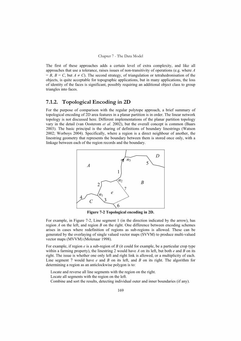
Chapter 7 - The Data Model
169
The first of these approaches adds a certain level of extra complexity, and like all approaches that use a tolerance, raises issues of non-transitivity of operations (e.g. where A = B, B = C, but A ≠ C). The second strategy, of triangulation or tetrahedronisation of the objects, is quite acceptable for topographic applications, but in many applications, the loss of identity of the faces is significant, possibly requiring an additional object class to group triangles into faces.
7.1.2. Topological Encoding in 2D For the purpose of comparison with the regular polytope approach, a brief summary of topological encoding of 2D area features in a planar partition is in order. The linear network topology is not discussed here. Different implementations of the planar partition topology vary in the detail (van Oosterom et al. 2002), but the overall concept is common (Baars 2003). The basic principal is the sharing of definitions of boundary linestrings (Watson 2002; Worboys 2004). Specifically, where a region is a direct neighbour of another, the linestring geometry that represents the boundary between them is stored once only, with a linkage between each of the region records and the boundary.
A
B
e
D
C
2
1
3 4
5
7
6
n1
n2
n3
Figure 7-2 Topological encoding in 2D.
For example, in Figure 7-2, Line segment 1 (in the direction indicated by the arrow), has region A on the left, and region B on the right. One difference between encoding schemes arises in cases where redefinition of regions as sub-regions is allowed. These can be generated by the overlaying of single valued vector maps (SVVM) to produce multi-valued vector maps (MVVM) (Molenaar 1998).
For example, if region e is a sub-region of B (it could for example, be a particular crop type within a farming property), the linestring 2 would have A on its left, but both e and B on its right. The issue is whether one only left and right link is allowed, or a multiplicity of each. Line segment 7 would have e and B on its left, and B on its right. The algorithm for determining a region as an anticlockwise polygon is to:
Locate and reverse all line segments with the region on the right. Locate all segments with the region on the left. Combine and sort the results, detecting individual outer and inner boundaries (if any).
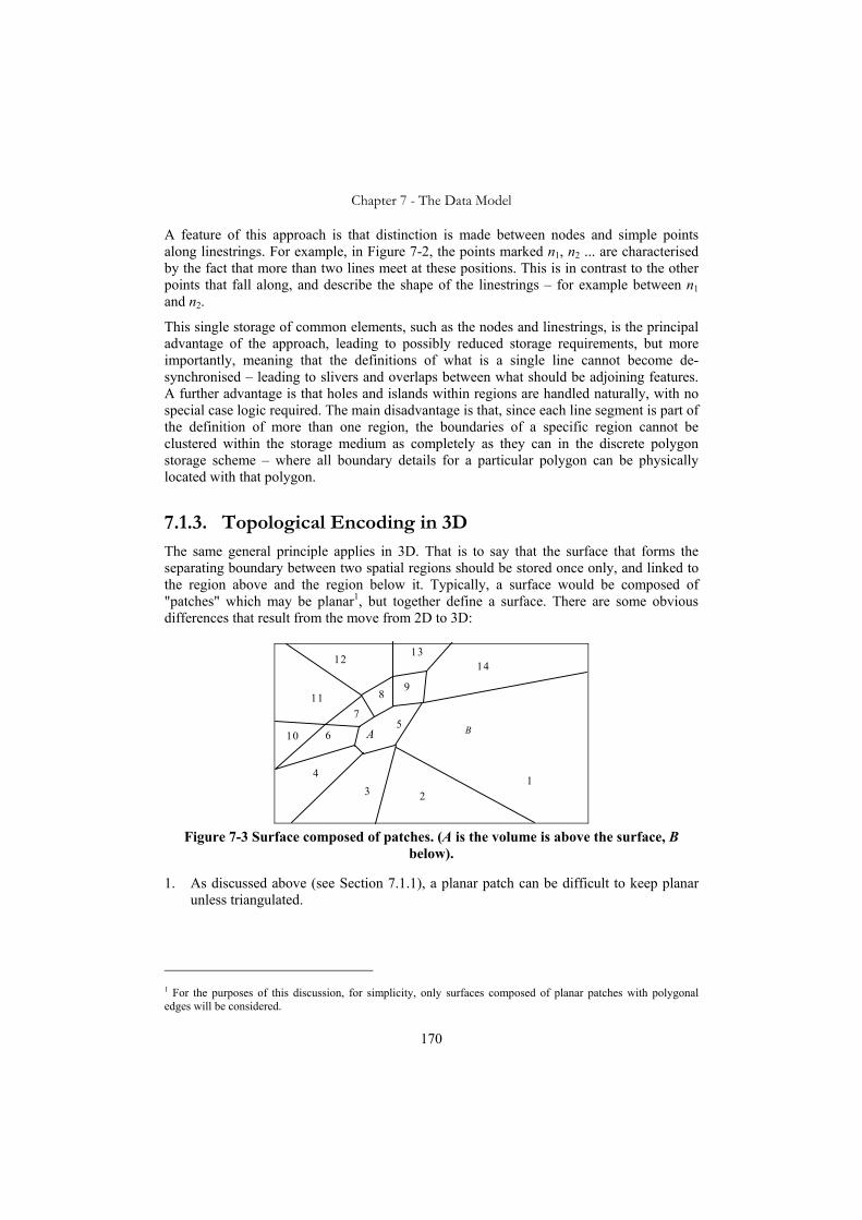
Chapter 7 - The Data Model
170
A feature of this approach is that distinction is made between nodes and simple points along linestrings. For example, in Figure 7-2, the points marked n1, n2 ... are characterised by the fact that more than two lines meet at these positions. This is in contrast to the other points that fall along, and describe the shape of the linestrings – for example between n1 and n2.
This single storage of common elements, such as the nodes and linestrings, is the principal advantage of the approach, leading to possibly reduced storage requirements, but more importantly, meaning that the definitions of what is a single line cannot become de-synchronised – leading to slivers and overlaps between what should be adjoining features. A further advantage is that holes and islands within regions are handled naturally, with no special case logic required. The main disadvantage is that, since each line segment is part of the definition of more than one region, the boundaries of a specific region cannot be clustered within the storage medium as completely as they can in the discrete polygon storage scheme – where all boundary details for a particular polygon can be physically located with that polygon.
7.1.3. Topological Encoding in 3D The same general principle applies in 3D. That is to say that the surface that forms the separating boundary between two spatial regions should be stored once only, and linked to the region above and the region below it. Typically, a surface would be composed of "patches" which may be planar1, but together define a surface. There are some obvious differences that result from the move from 2D to 3D:
A B
1
7
6 5
4 3 2
1312
11
10
98
14
Figure 7-3 Surface composed of patches. (A is the volume is above the surface, B
below).
1. As discussed above (see Section 7.1.1), a planar patch can be difficult to keep planar unless triangulated.
1 For the purposes of this discussion, for simplicity, only surfaces composed of planar patches with polygonal edges will be considered.

Chapter 7 - The Data Model
171
2. There is no natural ordering of the patches that compose a surface (by contrast with the line segments that comprise a linestring), e.g. in Figure 7-3, there is no reason the patches should be numbered as they are.
3. There is no 1-1 correspondence between patches and the edges (as there is in 2D between edges and points that define them), e.g. in Figure 7-3, patch 5 has seven edges.
As a result, there is significantly more variation in the proposed implementations of 3D topology than is the case in 2D (Breunig and Zlatanova 2006), for example, in the 3D FDS (Formal Data Structure) (Molenaar 1990), and the “Simplified Spatial Model” (SSM) (Zlatanova et al. 2002).
7.1.4. Storage Requirements In order to make comparisons with the data models discussed below, some representative vector based schemata have been analysed, with the details of the assumptions and calculations being given in Appendix VII.
Case 1: A 2D conventional polygon stored with no topological connection to neighbours.
Case 2: A 2D polygon stored as part of a single layer coverage with topology. Each polygon has on average 4 direct neighbours.
Case 3: A 3D conventional polyhedron stored with no topological connection to neighbours.
Case 4: A 3D polyhedron stored as part of a single layer partition of space with 6 direct neighbours. The figure being considered is a distorted cube – with 6 surfaces, 8 corner vertices, 12 edge line segments. The six surfaces are broken up into a number of surface patches.
In each case, three objects are considered, the first being of limited complexity – a 4-sided polygon in 2D or a 6-face polyhedron in 3D. The second has 100 vertices, while the third has 10000 vertices. The storage requirements of these cases are tabulated in Appendix VII, and will be quoted below in comparison with various regular polytope storage schemata.
7.2. The Discrete Regular Polytope Model This is perhaps the simplest structure, with the most redundancy of storage, and no topological encoding. Each regular polytope is stored as a unit, containing its component convex polytopes and their defining half spaces.

Chapter 7 - The Data Model
172
RegularPolytope
ConvexPolytope
Face
*
*
1
3..*
HalfSpace A, B, C, D: integer
Vertex
x, y, z: dr-rational
Regular Polytope Representation
Redundant Data
1
Possibly not stored in database, but derived as needed
Figure 7-4 The regular polytope model (see also Thompson 2005a).
Figure 7-4 shows, in the unified Modelling Language (UML) (OMG 1997), a possible implementation of the regular polytope representation discretely encoded (in 3D). Key points in the interpretation of this diagram are that:
• The ConvexPolytope class is a specialization of RegularPolytope.
• The HalfSpace class is a specialization of ConvexPolytope (which means it is also a RegularPolytope).
• A regularPolytope object consists of zero or more convexPolytopes. Note that zero defines the empty RegularPolytope.
• A convexPolytope object consists of zero or more halfSpaces. Note that zero defines the infinite ConvexPolytope.
• The HalfSpace class has the integer attributes A, B, C and D.
The face and vertex objects are derivable from the regularPolytope, convexPolytope and halfSpace objects, and therefore are redundant. It is an implementation decision whether they are stored in the database or not.
• Each halfSpace object corresponds to exactly one face.
• Each face object is composed of three or more vertices (some of which may be “at infinity” – see Section 4.1.3 definition 4.13).

Chapter 7 - The Data Model
173
• Each vertex carries as attributes the dr-rational x, y and z values of its coordinates.
The "Face" and "Vertex" object classes are not necessary to the definition of a regular polytope, but as discussed below may be of use in improving the performance of the implementation. Since these faces and vertices will need to be calculated in a range of operations, the calculation times may be sufficient to justify the additional storage required by what is in effect a materialised view in the database. This decision needs to be based on experimental evidence (see Chapter 8). The algorithm for the calculation of faces and vertices is, in outline:
For each convex regular polytope in the regular polytope definition, calculate the intersections between the half planes that compose it and form a set of conventional polygons. There will be one polygon for each original half space unless the half-space was redundant (and can be removed). These polygons are assembled to form a conventional convex polyhedron.
A
a B
Figure 7-5 Calculation of polygonal faces of a convex polytope. Note that half space B
is redundant – therefore does not generate a face.
In Figure 7-5, face a is calculated by intersection of half space A with the other half spaces of this convex polytope. Note that the half space B contains all the other vertices, and is redundant, so no face is generated. B can therefore be dropped from the convex polytope definition. The vertex test for redundancy (see Section 4.4.3 and Appendix IV.1) is useful in detecting such half spaces, and the complexity of the routines that are needed to determine redundancy are discussed in Chapter 8.
Given this and other forms of the regular polytope data model, there is the potential to include attributes within the regularPolytope, convexPolytope and halfSpace objects. This ensures a very flexible attribution structure, allowing, for example, attributes such as surface cover, quality of data, reflectance, texture etc. to apply only to specified surfaces of a solid.
The model as described here makes no distinction between connected and disconnected regular polytopes. It is possible to calculate whether a regular polytope is connected or not, but it may be worthwhile pre-calculating and storing this fact (for both weak and strong connection). This was done in the proof of concept Java classes described in Chapter 8 (see Section 8.2.2) to give instant determination of connectivity.

Chapter 7 - The Data Model
174
A2
A1
B
Figure 7-6 Calculating the intersection of two regular polytopes.
In calculating the intersection of region B with region A in Figure 7-6 (shown above split into two convex polytopes A1 and A2), even though all the half planes which define A1 intersect all the half planes that define B (since they are not parallel, and the half-plane definition is theoretically infinite), it can be determined by a conventional polygon overlap test that all the vertices of A1 are completely separated from the vertices of B – therefore A1∩B is empty. This kind of logic can be used to pre-eliminate large numbers of the partial intersections. (This could be preceded by a comparison of bounding boxes, to further improve the calculation speed).
7.2.1. Model Restrictions This model is the most basic, intended for demonstration purposes only. In practice, additional classes would be added to improve speed and responsiveness. For example, a convex polygon might be associated with an approximate bounding rectangle, which is the basis for a spatial index. Note that the bounding box can be computed with a function and that the spatial index may be created on the return value of that function. That is, the bounding box need not be stored if a functional spatial index is used.
A demonstration system has been developed in Java based on this simple model and is discussed in Chapter 8. There are a number of issues remaining that apply to this base level model:
• The regular polytope storage mechanism differs from the more familiar point/line/polygon/polyhedron paradigm commonly used in GIS, and requires non-trivial conversion routines to allow interoperability.
• The calculation of vertices requires the use of very large precision integer arithmetic (as does the dual grid approach, and to an even larger extent, the rational polygon - see Chapter 3).
• The storage requirements are larger than required for simple polygon/polyhedron encoding (even if redundant storage of faces and vertices is not used). (This is roughly quantified in Section 7.2.3 Table 7-1).
• It is not easy to map this storage form to/from the topological encoded form of a polygonal partition of space (Louwsma 2003). (This was discussed in Section 5.6).

Chapter 7 - The Data Model
175
• Some analytic operations, such as those that require volumes, areas etc., are inconvenient in the regular polytope representation (requiring significant processing). This can be alleviated by storing the redundant face and vertex objects.
7.2.2. Model Advantages
• Data retrieval can readily be optimised since each regular polytope can be stored as an individual self-contained record on disc, and indexed using standard techniques such as R-Tree (Guttman 1984).
• All RCC and topological predicates and functions can be rigidly supported in the computer-based representation.
7.2.3. Storage Requirements For comparison with the conventional approaches, as discussed in Section 7.1.4, six examples are considered as tabulated below:
Table 7-1: Independent (Non-topological) Storage
Vertex Defined Regular Polytope
2D, 4 sides 96 bytes2 144 bytes3
2D, 100 sides 864 bytes 1860 bytes
2D, 10000 sides 80 kb 165 kb
3D, 6 faces 404 bytes4 212 bytes5
3D, 100 faces 5686 bytes 2344 bytes
3D, 10000 faces 560 kb 207kb
In Table 7-1, it can be seen that in 2D the regular polytope requires rather more than twice the storage of the conventional approach. By contrast, this is a reduction of the storage in comparison to the conventional simple polyhedron structure in 3D. This should be treated with some caution, since the structure used for estimation has a lot of redundancy, and would not be likely to be used in a practical database. It should be noted that in this very simple schema there is little difference in storage requirements between the 2D and the 3D regular polytopes.
2 The schema used for these estimates can be found in Appendix VII.3.1. 3 The schema used for these estimates can be found in Appendix VII.4.1. 4 Note – this is a completely redundant form of storage, where each vertex is stored for each face of each polyhedron. See Appendix VII.3.3 for details of the schema assumed. 5 The schema used for these estimates can be found in Appendix VII.4.2.

Chapter 7 - The Data Model
176
7.3. Topological Encoding of Regular Polytopes In the storage schemes that are appropriate to the regular polytope representation, there are several possible analogues to topological encoding, but one in particular is quite promising for use in the field of cadastral data (Figure 7-7). This approach treats each half space as a common object, stored once only (in the way a common boundary is as described in Section 7.1.2), with links to each convex polytope that it bounds. The convex polytope may be bounded by the half space or by the complement of the half space.
A, B, C, D extents
* 1..*
complement: Boolean
HalfSpace
Orientation RegularPolytope
ConvexPolytope *
Figure 7-7 Regular polytope schema with common storage of half spaces.
As an example from the cadastral domain, consider a series of property parcels with a common road frontage as depicted in Figure 7-8. The single halfSpace XY participates in the definition of the road, and its complement in the convex polytopes A, B1, C1, D and E1. This ensures that:
• There are no gaps or overlaps possible between the parcels and the road.
• The road frontages are straight.
Since the true definition of the parcels from the survey plan was probably in terms of a bearing and distance measurement from point X to point Y, this is a particularly appropriate representation, and allows the option of storing such measurement details as metadata within the halfSpace record. This halfSpace XY would be linked by the direct connection to the road section 1, and via the “complement = true” link to convex polytopes A, B1, C1, D and E1. Note that halfSpaces can be used more than twice, in contrast to the traditional encoding of topology based on edges, where a common edge is always exactly used twice (positive and negative).

Chapter 7 - The Data Model
177
X
Y
A B1
B2 C1
C2 D E1
E2 F
G
Road 1
2 3
W
Z
Figure 7-8 Cadastral data in the topologically encoded regular polytope form.
Even where straight sections of frontage are non-contiguous, the halfSpace record can be used in common. For example, the halfSpace marked YZ defines the road section 2, with its complement defining E1, F, road section 3, G etc.
A
B1
C1
D
E1
F
X - Y
G
Road1
Road2
Road3
Y - W
Y - Z
C
C
C C
C
C C
C C
C
Convex Polytopes
Half Spaces Convex Polytopes
Figure 7-9 Object diagram showing some of the connections in Figure 7-8. (The
linkages marked "C" are links with “complement = true” as in Figure 7-7).
In full 3D parcels, the same is possible, with a half space being able to define a number of parcels in strata, as well as defining a non-stratum (2D) parcel adjoining it. In Figure 7-10, the half space marked as XY, is the boundary of “2D parcel” A, and its complement is the boundary of strata parcels B1 to B5.
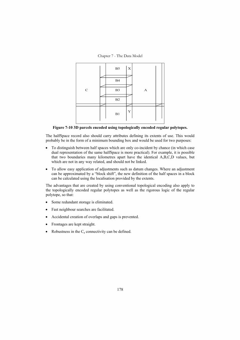
Chapter 7 - The Data Model
178
A
B1
C
B2
B3
B4
B5 X
Y
Figure 7-10 3D parcels encoded using topologically encoded regular polytopes.
The halfSpace record also should carry attributes defining its extents of use. This would probably be in the form of a minimum bounding box and would be used for two purposes:
• To distinguish between half spaces which are only co-incident by chance (in which case dual representation of the same halfSpace is more practical). For example, it is possible that two boundaries many kilometres apart have the identical A,B,C,D values, but which are not in any way related, and should not be linked.
• To allow easy application of adjustments such as datum changes. Where an adjustment can be approximated by a “block shift”, the new definition of the half spaces in a block can be calculated using the localisation provided by the extents.
The advantages that are created by using conventional topological encoding also apply to the topologically encoded regular polytopes as well as the rigorous logic of the regular polytope, so that:
• Some redundant storage is eliminated.
• Fast neighbour searches are facilitated.
• Accidental creation of overlaps and gaps is prevented.
• Frontages are kept straight.
• Robustness in the Ca connectivity can be defined.

Chapter 7 - The Data Model
179
H1
H2
H3 H4
H5
H6 H7
H8
H9
H10
H11 H12
H13
H14
C1
C2
C3
C4
H15
H16
Figure 7-11 Perturbation of connected objects preserving connectivity
The final point in the above list is significant. As was discussed in Section 5.7.3, Ca connectivity is naturally not a robust concept, and Cb connectivity is only robust if the adjacent anti-equal half spaces can be guaranteed to remain anti-equal. This form of topological encoding can ensure that truly robust connectivity is possible in both forms, since the anti-equal pair of half spaces is stored and can be manipulated as a single object. For example, in Figure 7-11, Even though both figures are perturbed, since the common anti-equal pairs (H2, H5) (H3, H6) and (H10, H13) are stored in common they are maintained as anti-equal. Thus the connectivity can be robust.
It is unlikely that there will be much, if any, saving in storage requirements using this structure, since the cost of storing a halver redundantly is quite low, and largely offset by the keys and indexing needed to support the encoding. This is also true of the conventional form of topological encoding, and in both approaches the advantages are not to be found in storage savings, but in the ease of update, while retaining correct adjacency (consistency within the model).
As a minor but significant variant on this approach, the whole of space can be subdivided into convex polytopes, which are grouped into regular polytopes, thus forming a complete partition of space equivalent to a restricted form of cellular model as described by Bidarra et al (1998). In such a partition, all half spaces (apart from the half spaces at infinity) will be present as an anti-equal pair, and an efficient storage regime should result.
7.3.1. Storage Requirements For comparison with the vertex representations approaches, as discussed in Section 7.1.4, six examples are considered, as tabulated in Table 7-2. These compare a topologically encoded vertex representation in 2D and 3D with the shared half space regular polytope encoding.
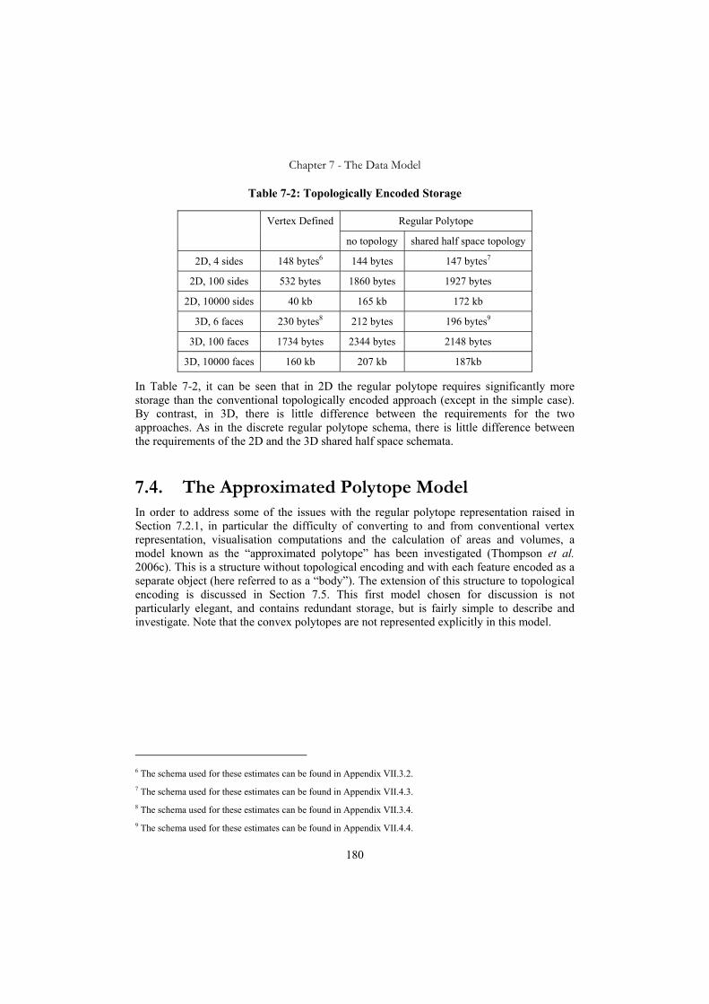
Chapter 7 - The Data Model
180
Table 7-2: Topologically Encoded Storage
Regular Polytope Vertex Defined
no topology shared half space topology
2D, 4 sides 148 bytes6 144 bytes 147 bytes7
2D, 100 sides 532 bytes 1860 bytes 1927 bytes
2D, 10000 sides 40 kb 165 kb 172 kb
3D, 6 faces 230 bytes8 212 bytes 196 bytes9
3D, 100 faces 1734 bytes 2344 bytes 2148 bytes
3D, 10000 faces 160 kb 207 kb 187kb
In Table 7-2, it can be seen that in 2D the regular polytope requires significantly more storage than the conventional topologically encoded approach (except in the simple case). By contrast, in 3D, there is little difference between the requirements for the two approaches. As in the discrete regular polytope schema, there is little difference between the requirements of the 2D and the 3D shared half space schemata.
7.4. The Approximated Polytope Model In order to address some of the issues with the regular polytope representation raised in Section 7.2.1, in particular the difficulty of converting to and from conventional vertex representation, visualisation computations and the calculation of areas and volumes, a model known as the “approximated polytope” has been investigated (Thompson et al. 2006c). This is a structure without topological encoding and with each feature encoded as a separate object (here referred to as a “body”). The extension of this structure to topological encoding is discussed in Section 7.5. This first model chosen for discussion is not particularly elegant, and contains redundant storage, but is fairly simple to describe and investigate. Note that the convex polytopes are not represented explicitly in this model.
6 The schema used for these estimates can be found in Appendix VII.3.2. 7 The schema used for these estimates can be found in Appendix VII.4.3. 8 The schema used for these estimates can be found in Appendix VII.3.4. 9 The schema used for these estimates can be found in Appendix VII.4.4.

Chapter 7 - The Data Model
181
composed of
Body
Face
A, B, C, D: int
4..*
Boundary
11..*
Edge
3..*
ApproximatedPoint
X, Y, Z: int1
ExactPoint1
DrRationalNumber
I, J: extended integer 3
Only during calculations
1
3..*
bounded by
limited by other facereverse of /derived
/derived
/derived
/derived
Figure 7-12 The simplified model
The classes are:
Body: is the volume of space which represents a feature. This can represent any regular polytope, not necessarily internally connected.
Face: is a geometrically flat facet of the bounding surface(s) of a body. (Note – a body can have internal surfaces – faces of an inner shell – like the interior of a tennis ball).
Boundary: is a planar ring which defines the edges of a face, stored anticlockwise for an outer boundary, clockwise for inner - as viewed from outside the body. (For an inner face, the outermost boundary will be anticlockwise, when viewed from within the void).
Edge: is a single directed line segment in a boundary – there will always be a pair of opposite edges for the junction of two faces.
ApproximatedPoint: is a representation of the points where faces meet. These would be stored redundantly, and assist with the fast approximate results (see below).
ExactPoint: is an exact representation of the intersection of three faces, the face with which it is stored, and the “other face” of the two edges that meet at this point. It is represented as a set of 3 dr-rational numbers. Exact points would not be stored in the database, being only used when intersection or union operations are being calculated.
DrRationalNumber: is a representation of a dr-rational number. It consists of two extended precision integers –M' ≤ I ≤ M', 0 < J ≤ M", interpreted as I/J.

Chapter 7 - The Data Model
182
The associations are:
Body “bounded by” face – to link the body to the faces that define it.
Face “limited by” boundary – each face is limited by one or more boundaries.
Boundary “composed of” edges – each boundary is a ring comprised of a connected set of edges.
Face “other face” of Edge – each edge is defined as the intersection of the face it defines with another face. Note – this relation is not defined for the purpose of carrying topological connectivity. It is purely to define the edge.
Edge “reverse of” Edge – each edge has another which is the exact reverse of it, the start and end points are identical (but reversed), and the boundary face of one will be the “other face” of the other (and vice versa). This relationship would probably not be explicitly stored.
Figure 7-12 shows a simplified model for discussion here. A body is considered to be defined by a number of faces. Each face has attributes of A, B, C and D, with the same interpretation as half spaces (see Chapter 4) and is bounded by one or more boundaries (with at least one being an outer boundary). An edge is the junction of exactly two faces, and defines the boundary of one of them. (Note that edges are thus stored twice, but each edge has just one point. This will be discussed further in Section 7.4.3).
Since the aim of this representation is to support the operations of the regular polytope, and the regular polytope is not necessarily fully bounded, it is necessary to define “faces at infinity” based on the half spaces at infinity H1
∞ (see Chapter 4 definition 4.13). Likewise, points with one or more of the x,y,z coordinates equal to ±M are considered to be “points at infinity”. The universal regular polytope O∞ can be represented as a body object (the universal box B∞), with six faces. Each face has a single outer boundary consisting of four edges. Each edge starts and ends at a point at exactly (±M, ±M, ±M).
The point-set definition of a body is simply the set of points which satisfy the “point in body” test. Briefly, for point p = (xp, yp, zp), this consists of running a ray in the -x direction, from the point and counting the faces it cuts. A face is deemed to be cut if the x intercept on this ray is ≤ xp. (note the equality is included). To cut a face, the point of intersection of the ray on the face must be within the boundaries of the face. This is tested by running a ray in the –y direction along the face, and counting the boundary edges it cuts. An edge is deemed to cut this ray if the y intercept is ≤ yp. The edge must also be such that zmax > zp and zmin ≤ xp where zmax and zmin are the max and min z values of the edge. Note – the detail of the use of > and ≤, and the direction of the rays is important in showing the equivalence of this approach with the regular polytope approach, but other strategies could be adopted – such as running in the –z direction first if this were not an issue.
In order to ensure that the rigorous logic of the regular polytope can be transferred to this representation it is necessary to show either that:
This representation can be mapped reliably to and from the regular polytope representation, or
The operations union, intersection and inverse can be implemented rigorously.

Chapter 7 - The Data Model
183
Clearly, 1 => 2 above, since if two-way mappings are available, then union, intersection and inversion can be implemented by mapping to the regular polytope representation, applying the operation, and then mapping back.
The other side of the equivalence (2 => 1) can be shown by considering the following:
By calculating where the half space H = (A,B,C,D) intersects the universal box B∞, a body can be generated BH. Thus a half space can be represented as a body, as shown in Figure 7-13. The body that represents a half space can have from four to seven faces. It can readily be verified that if p = (x,y,z) ∈ H, (-M ≤ x,y,z < M) ⇔ p ∈ BH.
H
BH
xy
z
(M,M,-M)
(M,M,M)
(-M,-M,-M)
B∞
Figure 7-13 The universal box B∞, and a half space H represented as a body BH.
If iniHC
..1== I is a convex polytope, and Bi is the body representation of Hi, then we can
define ini
C BB..1=
= I as the body representation of C. It can readily be verified that p ∈ C ⇔
p ∈ BC. By a similar argument, the union of any set of convex polytopes can be represented as a body. Therefore any regular polytope can be represented as a body using this structure.
In the reverse direction, if a body is convex (that is all faces meet at edges so that the dihedral angle of that meeting is less than 180°), then the body defines exactly that set of points which would be defined by a convex polytope bounded by the faces.

Chapter 7 - The Data Model
184
Convex region
Dihedral angle
Figure 7-14 Convex body defining a convex polytope.
For a non-convex body, if m pairs of faces meet at a dihedral angle of > 180°, then one of those faces can be converted into a half space and its inverse, and therefore into a complementary pair of bodies that covers the universal box. The original body is then replaced by two bodies – each being the intersection of the original body with one of the complementary pair. By this process, two bodies are created that each have at most m-1 pairs of faces with dihedral angle of > 180°. Continuing this process, we are left with a set of convex bodies whose union is the original body. This can then be expressed as a regular polytope (see Figure 7-15).
A
H1
AB
H1
H2
A B
C
Non-convex body with two planes of concavity
One concavity resolved, by splitting along H1
Second concavity resolved, by splitting along H2
Figure 7-15 Cutting a non-convex body into convex sub-regions.
Using dr-rational arithmetic, the operations of union, intersection and inverse can be defined, and by careful considerations of the rules of inclusion, it can be verified that the results of the operations are consistent with the results of those same operations on the regular polytope representation. Thus this representation is logically equivalent to the regular polytope. It can therefore be asserted that this approach supports the algebras discussed in Chapter 6. The use of dr-rational numbers requires some care in the specification of the algorithms, since it is necessary to verify that the results of any calculations do not violate the domain limits, but the algorithms themselves are significantly simpler than those often employed in floating point arithmetic, because no calculation or rounding errors need be accommodated.

Chapter 7 - The Data Model
185
7.4.1. The Approximation The approach has been called “approximated polytope”, but so far, all discussion has been of exact operations. The approximation takes the form of an approximated point – stored instead of the dr-rational points. This allows a form of the body representation to be available for “everyday use”. It is envisaged that these points would be used for visualisation, the analytic operations (overlap, proximity, containment etc), geographic search and indexing and other such purposes. In fact, all operations except those involving the exact generation of new objects. It is possible for these approximated points to be stored in integer or floating point form, at whatever accuracy is desired, and the calculation of them from dr-rational numbers can be highly accurate. If integers are used, the approximated point may be determined to within one unit of resolution of the exact point in x, y, and z.
Using the “point within body” test as described above, but using the approximated points for calculation (and not needing dr-rational arithmetic), it can be seen that the correct result will be obtained provided the test point is not within one unit of resolution of the surface of the body. It can further be seen that it is possible to determine whether the point is within a specified distance from the surface. It is thus possible to convert from this representation to a more conventional (point location based) representation, simply by using these approximated points. Note however that while the faces themselves are flat by definition, the approximated points may lie up to one unit of resolution off the flat plane, so the usual issues of faces defined by more than three points not being planar will then apply (see Figure 7-16). It is also the case that two or more points may approximate to the same value, so the interpretation into conventional form must be carefully approached (see Section 7.4.3).
Figure 7-16 Approximated points used in place of dr-rational vertices.
The presence of approximated vertices within the representation makes the application of this approach to classic GIS-type analysis considerably simpler. The accuracy of the approximation is high, and for such operations as the calculations of areas, volumes, linear sizes, distance between objects, etc. they would be appropriate in the vast majority of cases. In addition, operations such as overlap, containment, above/below, within (convex hull), etc. can be implemented using conventional (and well optimised) algorithms. All of these will be accurate to within the basic grid size, and therefore valid for the majority of analysis work.
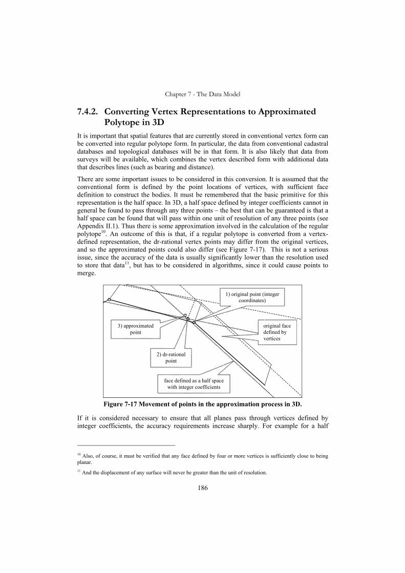
Chapter 7 - The Data Model
186
7.4.2. Converting Vertex Representations to Approximated Polytope in 3D
It is important that spatial features that are currently stored in conventional vertex form can be converted into regular polytope form. In particular, the data from conventional cadastral databases and topological databases will be in that form. It is also likely that data from surveys will be available, which combines the vertex described form with additional data that describes lines (such as bearing and distance).
There are some important issues to be considered in this conversion. It is assumed that the conventional form is defined by the point locations of vertices, with sufficient face definition to construct the bodies. It must be remembered that the basic primitive for this representation is the half space. In 3D, a half space defined by integer coefficients cannot in general be found to pass through any three points – the best that can be guaranteed is that a half space can be found that will pass within one unit of resolution of any three points (see Appendix II.1). Thus there is some approximation involved in the calculation of the regular polytope10. An outcome of this is that, if a regular polytope is converted from a vertex-defined representation, the dr-rational vertex points may differ from the original vertices, and so the approximated points could also differ (see Figure 7-17). This is not a serious issue, since the accuracy of the data is usually significantly lower than the resolution used to store that data11, but has to be considered in algorithms, since it could cause points to merge.
1) original point (integer coordinates)
2) dr-rational point
3) approximated point
original face defined by vertices
face defined as a half space with integer coefficients
Figure 7-17 Movement of points in the approximation process in 3D.
If it is considered necessary to ensure that all planes pass through vertices defined by integer coefficients, the accuracy requirements increase sharply. For example for a half
10 Also, of course, it must be verified that any face defined by four or more vertices is sufficiently close to being planar. 11 And the displacement of any surface will never be greater than the unit of resolution.

Chapter 7 - The Data Model
187
space to pass within 1 resolution unit of three points (defined by 4 byte integer coefficients):
• A, B and C must be 4 byte, and D must be 8 byte integers.
• The dr-rational numbers (p/q) used to represent vertices in this case p requires 16 bytes, and q requires 12 bytes, with equality testing needing 28 byte arithmetic.
If a half space is to pass exactly through three integer coefficient points:
• A, B and C need 8 byte, and D 12 byte integers.
• In this case, the requirement for p is 28 bytes, for q is 24 bytes, with equality testing needing 52 bytes.
A further issue is that an edge is defined by the meeting of exactly two faces. It is not possible in general to generate another face that passes through the edge of intersection of two existing faces (see Figure 7-18). This does not significantly affect the model being discussed here, but will have an impact on topological encoding (see Section 7.5.3 below).
existing faces
edge of intersection of existing faces
new face
Figure 7-18 In general, in 3D, a face cannot be guaranteed to pass through the edge of
intersection of two other faces.
Note that none of these issues apply in the 2D case. In 2D, for any two points with integer coefficients, a half plane can be generated that passes exactly through them. Thus, for a 2D vertex represented polygon, a regular polytope can be generated that exactly represents it (apart from those points that lie on the boundary of the original polygon).
7.4.3. Practical Questions It is considered unnecessary to store the exact dr-rational vertices in the database, since they can be recalculated as necessary in O(v) time, where v is the number of vertices. Since the dr-rational numbers are of finite precision, the operations are of constant duration (unlike the unrestricted rational numbers, where the time of calculation of arithmetic operations depends on the magnitude of the numerators and denominators). Calculations using dr-rational numbers in demonstration classes (see Chapter 8) implemented in Java are quite slow, since for ease of implementation they have used the readily available BigInteger

Chapter 7 - The Data Model
188
class, which is potentially infinite in precision. In a practical implementation a faster (finite) arithmetic could be used.
In the schema described here (in Figure 7-12), the edge of intersection between two faces is recorded as a pair of edge objects, one per face, each the reverse of the other. This is obvious duplication, and could be addressed in any practical implementation. (The described schema being for “proof of concept” only).
7.4.4. Storage Requirements For comparison with the vertex representations approaches, as discussed in Section 7.1.4, three cases are considered as tabulated in Table 7-3. These compare a topologically and non-topologically encoded vertex representation 3D with the approximated regular polytope (non topological) encoding. It was not considered to be useful to compare the 2D cases, since the 2D and 3D requirements for the regular polytope are fairly similar.
Table 7-3: Approximated Polytope Storage
Non-Topo see Appendix VII.3.3
Topo see Appendix VII.3.4
Approximated Polytope see Appendix VII.4.5
3D, 6 faces 404 bytes 230 bytes 620 bytes
3D, 100 faces 5686 bytes 1734 bytes 9268 bytes
3D, 10000 faces 560 kb 160 kb 920 kb
In Table 7-3, it can be seen that in all cases, the approximated regular polytope requires significantly more storage than the conventional encoded approaches. This schema also requires a considerable increase in storage over the earlier regular polytope approaches and is only justified if the speed improvement over them is significant. The large storage requirement is a function of the large amount of redundancy that this approach incorporates.
7.5. Extension to Topological Encoding The approximated polytope has a significant amount of redundancy in storage, and a topologically encoded form of storage must be considered. As with conventional vertex-represented structures, this could take several forms, two of which are considered here. The principal investigation of these has been in 3D, since this is the more complex case. The 2D equivalents follow fairly obviously by comparison.
7.5.1. Shared HalfSpace Topology One possible form of topology for the approximated polytope model is the equivalent to that described in Section 7.3. Figure 7-19 shows a simplified model for discussion here. A
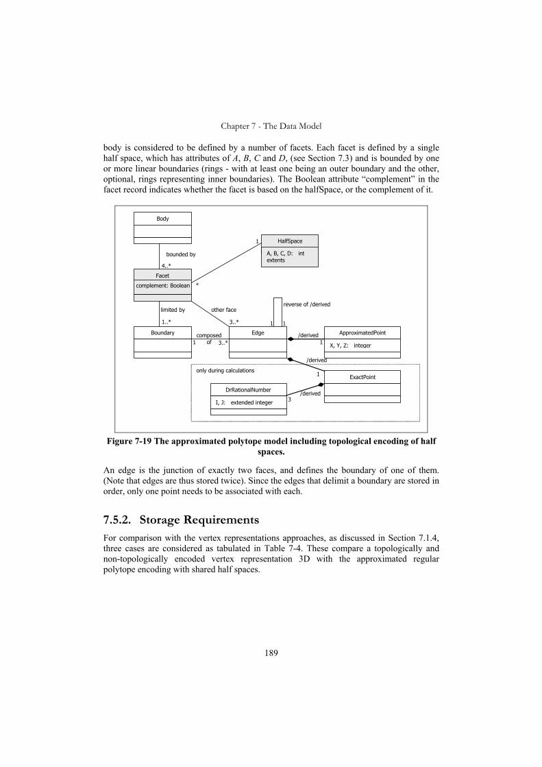
Chapter 7 - The Data Model
189
body is considered to be defined by a number of facets. Each facet is defined by a single half space, which has attributes of A, B, C and D, (see Section 7.3) and is bounded by one or more linear boundaries (rings - with at least one being an outer boundary and the other, optional, rings representing inner boundaries). The Boolean attribute “complement” in the facet record indicates whether the facet is based on the halfSpace, or the complement of it.
Body
Facet
4..*
Boundary
11..*
Edge
3..*
1
ApproximatedPoint
X, Y, Z: integer1
ExactPoint1
DrRationalNumber
I, J: extended integer 3
only during calculations
1
3..*
bounded by
limited by
composed of
other facereverse of /derived
/derived
/derived
/derived
HalfSpace
A, B, C, D: intextents
complement: Boolean
1
*
Figure 7-19 The approximated polytope model including topological encoding of half
spaces.
An edge is the junction of exactly two faces, and defines the boundary of one of them. (Note that edges are thus stored twice). Since the edges that delimit a boundary are stored in order, only one point needs to be associated with each.
7.5.2. Storage Requirements For comparison with the vertex representations approaches, as discussed in Section 7.1.4, three cases are considered as tabulated in Table 7-4. These compare a topologically and non-topologically encoded vertex representation 3D with the approximated regular polytope encoding with shared half spaces.

Chapter 7 - The Data Model
190
Table 7-4: Approximated Polytope Storage
Vertex Representation Approximated Polytope
Non-Topo App VII.3.3
Topo App VII.3.4
Non-Topo AppVII.4.5
Shared HalfSpace Topo See Appendix VII.4.6
3D, 6 faces 404 bytes 230 bytes 620 bytes 626 bytes
3D, 100 faces 5686 bytes 1734 bytes 9268 bytes 9368 bytes
3D, 10000 faces 560 kb 160 kb 920 kb 930 kb
This is not significantly different from the version of regular polytope storage which does not share half spaces, and the use of this approach would be considered rather for its convenience in applying updates (as was discussed in Section 7.3).
7.5.3. Shared Surface Topology Figure 7-20 shows an alternative approach to topological encoding, which is more akin to the conventional vertex based approaches, and requires that a set of faces be grouped into a compound surface while bodies are defined by the surfaces that surround and separate them from other bodies. A surface is linked to the body above (+) or below (-) it.
Surface
Body
1..21..*
+ / -
Face
A, B, C, D: int
1..*
Boundary
1..* ApproximateEdge ApproximatedPoint
X, Y, Z: int
2* *left/right
Figure 7-20 The model including topological encoding.
The objects are:
Body: a volume of space
Surface: a 2D surface comprised of a series of flat faces which separates two bodies.
Face, Boundary and ApproximatedPoint are the same as defined in Section 7.4, but since the approximatedEdge objects are shared between boundaries, each edge must be linked to two approximatedPoint objects.

Chapter 7 - The Data Model
191
The edge is represented by the class:
ApproximatedEdge: an edge between two faces which may or may not be part of the same surface. Unlike the exact edge, this does not need an alternate face link. Also unlike the edge described in Section 7.4, this is shared between two or more boundaries objects.
The topological connectivity is provided in two ways – each body is linked to the surfaces that define it. These surfaces are in turn linked to the bodies on the other side. In addition, each nodal approximatedEdge object is linked (via the boundary, face and surface objects) to the three or more bodies that meet there.
A B
C
f4
s1
f5 n1
e1
f1
f2
f3
s4
s5 f6 Figure 7-21 Example of bodies, faces and edges.
For example, in Figure 7-21, bodies A and B are separated by surface s1, which is composed of faces f1, f2 and f3. A and C are separated by surface s4, which is composed of face f4. B and C are separated by surface s5 consisting of faces f5 and f6. ApproximatedEdge e1 is on the common boundary between the faces f1 and f2 and is thus within surface s1, while approximatedEdge n1 lies approximately along the faces f2, f4 and f5 and is considered nodal. The requirement is that a “nodal edge”, be defined as the meeting of three or more faces, which raises difficulty in the approximated polytope approach, since at most two faces can be guaranteed to meet exactly at a single edge (see Figure 7-18).
A
B
CS1
S2S3
e
f1f2
f3f4
Figure 7-22 Topological encoding of bodies by surfaces.
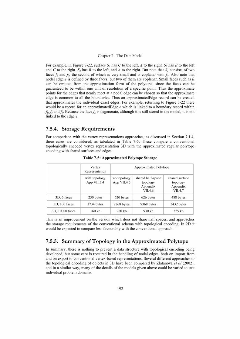
Chapter 7 - The Data Model
192
For example, in Figure 7-22, surface S1 has C to the left, A to the right. S2 has B to the left and C to the right. S3 has B to the left, and A to the right. But note that S1 consists of two faces f1 and f2, the second of which is very small and is coplanar with f3. Also note that nodal edge e is defined by three faces, but two of them are coplanar. Small faces such as f2 can be omitted from the approximation form of the polytope, since the faces can be guaranteed to be within one unit of resolution of a specific point. Thus the approximate points for the edges that nearly meet at a nodal edge can be chosen so that the approximate edge is common to all the boundaries. Thus an approximatedEdge record can be created that approximates the individual exact edges. For example, returning to Figure 7-22 there would be a record for an approximatedEdge e which is linked to a boundary record within f1, f3 and f4. Because the face f2 is degenerate, although it is still stored in the model, it is not linked to the edge e.
7.5.4. Storage Requirements For comparison with the vertex representations approaches, as discussed in Section 7.1.4, three cases are considered, as tabulated in Table 7-5. These compare a conventional topologically encoded vertex representation 3D with the approximated regular polytope encoding with shared surfaces and edges.
Table 7-5: Approximated Polytope Storage
Vertex Representation
Approximated Polytope
with topology App VII.3.4
no topology App VII.4.5
shared half-space topology Appendix
VII.4.6
shared surface topology Appendix
VII.4.7
3D, 6 faces 230 bytes 620 bytes 626 bytes 488 bytes
3D, 100 faces 1734 bytes 9268 bytes 9368 bytes 3432 bytes
3D, 10000 faces 160 kb 920 kb 930 kb 325 kb
This is an improvement on the version which does not share half spaces, and approaches the storage requirements of the conventional schema with topological encoding. In 2D it would be expected to compare less favourably with the conventional approach.
7.5.5. Summary of Topology in the Approximated Polytope In summary, there is nothing to prevent a data structure with topological encoding being developed, but some care is required in the handling of nodal edges, both on import from and on export to conventional vertex-based representations. Several different approaches to the topological encoding of objects in 3D have been compared by Zlatanova et al (2002), and in a similar way, many of the details of the models given above could be varied to suit individual problem domains.

Chapter 7 - The Data Model
193
7.6. Spatial Indexing of the Regular Polytope All of the variations on the regular polytope that have been described in this chapter share the need for spatial indexing. At the minimum, it is necessary to provide a fast algorithm to locate the representations of features that overlap or connect with a defined region. Fortunately this is relatively easy, using readily available indexing strategies such as the R-Tree (Guttman 1984). In this, as with many other strategies, the individual objects are represented in the index by limiting bounding boxes. The search proceeds in two parts. The index is used to determine a list of all objects that could possibly contact the search region. The second phase determines which objects do in fact satisfy the actual spatial predicate. For example, if all regular polytopes are wanted that are non tangential proper parts (NTPP) of a given search area, the bounding box is used to find all regular polytopes whose bounding rectangles intersect that of the search region.
This list could contain many other regular polytopes – some of which may overlap the area but not in an NTPP relationship. There may even be regular polytopes which are disjoint from the actual area. Since the calculation of the exact predicates is more expensive than calculation of overlap of rectangles, an index with good powers of discrimination is an advantage. Note that the bounding box or rectangle can be defined as a convex polytope, so that the rigour of the operations therefore applies.
The decision to be made in the regular polytope representation is whether to index the regular polytopes or the convex polytopes that comprise them (or both). The advantage of indexing only the regular polytope itself is that a more compact index results. The advantage with the convex polytope is that the index is more discriminating. In practice, this decision will be part of the database design decision required for any particular application. Note that if the disjoint normal form of the regular polytope is used (Section 4.1.5), the discrimination of a convex polytope based index is improved.
7.7. Relationship with Other Approaches Several schemata have been discussed, and in the process of investigation, certain properties of the representation have been developed. In particular, the approach known as the “approximate polytope” has been developed in various forms, which have a different appearance from the original regular polytope structure, but have the same algebraic behaviour.
In 2D, this approximated polytope has some parallels with the dual grid12 approach, and of the Queensland Digital Cadastral Data Base, which are discussed in this section.
12 See Section 3.4.4 for a summary of the dual grid approach.

Chapter 7 - The Data Model
194
7.7.1. Relationship of Approximated Polytope Approach with Dual Grid
The two approaches have much in common – both in effect use dr-rational numbers for the fine grid, and integers (or fixed-point numbers) for the coarse grid. In 2D, both have the same precision requirements.
Definition of Points, Lines, Polygons and Polyhedra
In 2D the approaches are very closely related with regard to the definition of polygons. The approximated polytope approach so far has not yet been extended to points and lines.
In 3D, there is a significant difference (if the natural extension of the dual grid to 3D is taken – defining the surfaces by lines and/or vertices as is done in 2D). The regular polytope approach (and therefore the approximated polytope approach) defines the surfaces as Ax + By + Cy + D = 0 with integer values of A, B, C, D. To define the surfaces by triples of integer-valued points would require another order of magnitude increase in the precision of arithmetic required to support it.
It is probably unfair to speculate on the extension of dual grid to 3D, since this has not been done yet and may take the face definition approach – but this does not seem to be in keeping with the 2D formulation. Also, the face definition formulation does not lend itself naturally to the dimensional boundary logic, which seems to underpin dual grid.
Algebra
The dual grid is what is here termed a vertex-defined representation, and has boundaries. A boundary of a 2D object is a set of 1D objects (lines). These lines are defined by two end points, and made up of a “lot of” intermediate points. Being a finite representation, the set of points on a line is not dense in the real number or rational number sense, but it contains every possible point where any other line (defined by integer coefficients) could intersect this line. (A “lot of” points - see 7.7.2 below).
Thus, for every polygon, there exists a point set which is its interior, a point set which is its exterior, and a point set which is its boundary. This is similar to the classic Euclidean space that is used to analyse much of the current geographic information theory. But it is not Euclidean.
The regular polytope – and therefore the approximated polytope representations do not have any points in the boundary – by virtue of the definition of the half space, and by virtue of the careful use of < vs ≥ in the definition of point containment. This means that the polygons in 2D, or polyhedra in 3D have only two point sets associated – the interior and the exterior. This allows their definition as regular sets, and also leads to the identification of the space as a Boolean algebra.
In generating an analogue for the region connection calculus (Randell et al. 1992) that allows for finite sets, (Roy and Stell 2002) make clear the fact that the definition of “part of” in terms of connection is untenable in a finite representation. These papers consider the dual grid approach in detail, and suggest a modification to the Boolean connection algebra (Stell 1999), which introduces a special type of region known as an atom, and replaces the

Chapter 7 - The Data Model
195
Boolean algebra axioms with those of a “dual pseudocomplemented distributive lattice” This does not necessarily possess a true complement, but has a dual pseudocomplement which satisfies (if R* is the dual pseudocomplement of R) R ∨ R* = 1 but not necessarily R ∧ R* = 0.
In this approach, an atom is distinguished from other types of region in that (by a side-effect of one of the axioms) an atom is part of its own dual pseudocomplement. This then leads to a connection algebra – which is no longer Boolean, and has the non-atomic axiom omitted. (B5. ),(:, yxCRyRx ¬∈∃∈∀ ).
This pseudocompliment is not necessary in the case of the approximated polytope or the regular polytope approach. The Boolean connection algebra can be used simply by omitting the non-atomic axiom (B5). The definition of “part of” in terms of connection is also untenable - but this must be the case for any finite representation (Roy and Stell 2002 page 283). Thus it can be stated that the approximated polytope – like the regular polytope approach is a “finite BCA” where this is taken to mean the BCA with the non-atomic axiom omitted.13
7.7.2. Note on Density of Points It is well known that there are significantly more irrational numbers than there are rational numbers, and that the rational numbers are dense. That is to say, for any interval, there is an infinite number of rational numbers in that interval.
The dr-rational numbers do not have this property, since there exist pairs of unequal dr-rational numbers that have none between them. For example the numbers 0 and 1/M' have no dr-rational numbers between (where M' is the largest denominator allowed).
They do, on the other hand possess a kind of density, because (in 2D) any line that can be represented that intersects the line we are considering, will intersect it at a dr-rational point. (This applies equally to the finer grid in the dual grid approach). In 3D, this is even more dramatic, because for any three planes, defined using integer coefficients A, B, C and D that meet at a real point p = (x,y,z) (-M≤ x,y,z < M); p is a representable dr-rational point. This means that the number of dr-rational points on any part of a plane surface is “very large” indeed, but, of course, still finite.
7.7.3. Relationship with the Queensland DCDB Structure The Queensland DCDB (Digital Cadastral Data Base) (NRW 2005) can be viewed as a boundary-free representation. Each parcel that makes up the base cadastral coverage is defined by its bounding vertices. Adjoining parcels are constrained by the update process so that their vertices in common have exactly the same (integer) representations (redundantly
13 I prefer to avoid the term “atomic BCA”, because there is no need to refer to atoms in its definition – merely omit the non-atomic axiom. In fact, both of these terms are flawed, because an infinite, non-atomic BCA by this definition would also be a “finite BCA” or an “atomic BCA”. A new term is needed! (“not-necessarily-infinite BCA”, “not-non-atomic BCA” or “possibly finite BCA” … “BCA-nA”)

Chapter 7 - The Data Model
196
stored). This is a very common form of storage, but the “boundary-free” characteristic comes from the definition of point-set inclusion.
Point p = (x,y) is considered to be within parcel A if the cut count c from the following algorithm is an odd number.
c ← 0; For each line (x1,y1) (x2,y2) of A If max(y1 , y2) ≥ y and min(y1,y2) < y If (y-y1)*(x2-x1) < (y2-y1)*(x-x1) Add 1 to c End if End if End for
This is just the usual Jordan curve test for inclusion, but it can be shown that every point within the region of interest lies, as determined by this test, within one and only one base parcel. This even applies to points that lie exactly on edges or vertices. It can be shown that these points will give the odd cut count for one parcel only.
This is an advantage in programming – because “find parcel at point” can be guaranteed to return a singleton in every case. It is possible to show that with a suitable definition of “part of”, and connectivity, the DCDB as implemented in Queensland can support the RCC8 relations. What this structure cannot support is a rigorous calculation of intersection, union and inverse (in common with most geographic information databases).
7.8. Summary of Data Volumes The estimated storage requirements of the various proposed schemata, are tabulated in tables 7.6 and 7.7 for convenience.
Table 7-6 - Vertex Representations 2D
Simple 2D
Moderate 3D
Large 3D
Simple 3D
Moderate 3D
Large No topology 96 b 864 b 80 kb 404 b 5668 b 560 kb
With topology 148 b 532 b 40 kb 230 b 1736 b 160 kb
Table 7-7 – Regular Polytope Representations 2D
Simple 2D
Moderate 3D
Large 3D
Simple 3D
Moderate 3D
Large No topology 144 b 1860 b 165 kb 212 b 2344 b 207 kb
Shared halver topology 147 b 1927 b 172 kb 196 b 2148 b 187 kb Approximated – no
topology 620 b 9268 b 920 kb
Approximated – with shared halver
626 b 9368 b 930 kb
Approximated – with shared surfaces
488 b 3432 b 325 kb
Chapter 7 - The Data Model
197
In summary, in 2D, the regular polytope can be expected to require slightly more than double the storage of the conventional polygon, while in 3D, the difference is not as pronounced.
7.9. Conclusions This chapter has defined and compared several alternative schemata to the database representation of spatial objects in regular polytope form. In addition to the basic schema, a version with topological encoding has been discussed. A major alternative, the approximated polytope, has also been introduced and some of its characteristics explored. The rigorous algebras discussed in Chapter 6 are all implemented by the regular polytope approach, and likewise by this approximated polytope model. Also common to both representations is a rigorous and calculable equality test.
The approximated polytope approach has in addition, advantages for visualisation and analytic predicates such as proximity, containment, overlap, above/below etc, where a degree of approximation is permissible, and where the existence of the approximate vertices allows for the conventional (and well optimised) algorithms to be used. The calculation of area, perimeter, volume and angular bearings is also simplified. Finally, it is possible to implement efficient layer overlay functionality with the approximated vertices being used for a “first cut”, eliminating those pairs of features which could not possibly overlap, and with the actual intersections of pairs of features being calculated rigorously.
Storage requirements have been considered, and it has been shown that, while in general, the regular polytope approaches (including the approximated variation) require more storage than conventional vertex representations, this difference is not particularly significant in view of the advantages that a rigorous algebra brings. Indexing has been considered, and the approaches have been compared with the dual grid and Queensland DCDB.
In the next chapter will be found the description of a set of “proof of concept” Java classes, which have been developed to investigate the algorithmic complexity of the structures defined in this chapter.


Chapter 8
Implementation Issues
The previous chapters have described the regular polytope, its logic and data models. The regular polytope has been shown to be a promising candidate for the rigorous representation of geometric objects in a form that is computable using the finite arithmetic available on digital computers. This is in contrast to the current practise where geometric algorithms are based on infinite precision mathematical axioms, which do fail in “exceptional” cases due to the finite digital arithmetic implemented by computers.
In order to explore practical issues in the regular polytope representation, a series of classes have been written in the Java programming language (Thompson and Van Oosterom 2006b), based on the simple model documented in Section 7.2 and cadastral features encoded using these classes have been stored using an Informix database. The data chosen were cadastral property boundaries, since large volumes of data were available, and this topic presents some unique challenges, in particular the mix of 3D and 2D data that is involved (Stoter 2004). The regular polytope representation provides a particularly elegant solution to this issue. In these Java classes, only the dr-rational interpretation of the regular polytope is addressed.
This chapter describes the implementation, and discusses some of the practical considerations that arose as a result, giving an indication of the requirements of a full implementation and what further development is needed. Section 8.1 explains the rationale for the choice of a problem domain for this proof of concept. Section 8.2 gives a summary of the Java classes that were developed for this study. Section 8.3 discusses the data used to test the concept. Section 8.4 concentrates on the complexity of the algorithms and their potential for practical implementation. Section 8.5 discusses the benefits that can be gained by careful implementation of the model and control of the regular polytope structure. Section 8.6 highlights the question of loading a database in the regular polytope format

Chapter 8 - Implementation Issues
200
from a source in conventional polygonal form. Section 8.7 summarises and concludes the discussion.
8.1. Rationale for the Approach Taken It was felt that, while the regular polytope can clearly be used to represent various geometric constructs, it is only by applying the representation to a practical problem that its true worth can be verified. For that reason, it was decided to load approximately a thousand cadastral parcels from the Queensland Cadastre, over a semi-urban region of average density and complexity. The region chosen contains primarily base (2D) parcels, but also has a smaller number of easements, and several 3D parcels. It consists of properties associated with residential, light commercial, light industrial, and recreational land usage.
The base cadastral parcels are known as 2D parcels, but as pointed out by Stoter (2004), the property is actually the right to a volume of space, with the height and depth restrictions not explicitly stated. Thus it is the representation of the property that is 2D, not the property right itself. The regular polytope, since it does not need to be bounded on all sides is a natural representation for a mix of 2D and 3D parcels – considering the 2D parcels as prisms with vertical sides and no defined top or bottom. It is quite meaningful in this context, to ask whether a 2D base parcel intersects a 3D volumetric parcel. For example in Figure 8-1, parcels A and B do not intersect C, but D and a section of road do. (The shaded area below C represent the “footprint” of C at the base level).
A B
C
D
Figure 8-1 Mixing 2D and 3D Cadastre.
The Java objects as developed parallel the definitions of the components of the regular polytope, and are categorised as:
• The half space (or half plane),
• The convex polytope,
• The regular polytope.

Chapter 8 - Implementation Issues
201
This object model is intended for manipulation purposes in the processing software, and so differs from the various models given in Chapter 7, which were intended primarily to illustrate a data storage strategy. The Java classes are set up to facilitate the mixing of 2 and 3 dimensional data.
This implementation only models 3D and 2D objects, with no extensions to either lower or higher dimensionality. An extension into the time dimension will be discussed in Section 10.2.2. Since this is intended to explore practical issues associated with cadastral data, no attempt has been made to produce a fully general n-dimensional model. Also there is no provision made for lower-dimensional objects (such as lines, points and surfaces) to be embedded in the space. A discussion of these issues will be found in Section 10.1.
8.2. Description of the Java Objects These classes and interfaces were developed to demonstrate the implementation of the logic defined in Chapter 6 for regular polytopes. The Java classes contain redundant information and constructs to assist with these calculations, which are not necessarily intended to be stored permanently and therefore not written to the database in this implementation. Likewise, links that are described below may not be of a permanent nature – for example the link marked “surrounded by” is not written to the database in the proof of concept coding.
8.2.1. Classes and Relations
surroundedBy
1
A, B, D: int; p1, p2: Point2R
HalfSpace 3..*
A, B, C, D: int; p: Point3R[3..*]
Halver
HalfPlane
Figure 8-2 The Halver, HalfSpace and HalfPlane classes.
As noted above, and as is clear from Figure 8-2, this implementation is restricted to 2D and 3D only – in line with the chosen problem domain. It would be possible to extend the dimensionality, and in particular to include the time dimension, but this is outside the scope of this thesis (see Section 10.2.2). The half space/plane object is characterised by classes based on the Halver as shown in Figure 8-2 described below:

Chapter 8 - Implementation Issues
202
HalfSpace: Defines a 3D half space (see Section 4.1.2), and carries the parameters A, B, C and D, which are integers – A, B and C requiring 32 bits and D requiring 64 bits. The array of dr-rational points p define the edges of the actual face of the convex polytope within this halfSpace boundary. These are for calculation purposes, and not written to the database.
HalfPlane: Defines a 2D half plane and carries the integer parameters A, B, and D. A and B require 32 bits and D requires 64 bits. Parameter C is not needed in 2D. The dr-rational points p1 and p2 define the ends of the edge within this halfPlane. These are for calculation purposes, and not written to the database.
Halver: An abstract class, from which the HalfSpace and HalfPlane classes are defined. This class is never instantiated.
Point2R and Point3R are dr-rational point classes. They consist of a tuple of rational numbers (2 or 3 respectively), each number consisting of a pair of integers (using the Java BigInteger). BigInteger is a convenient method of dealing with the large precision required by this approach, being effectively unlimited in precision. Unlimited precision is not strictly necessary, since the precision requirements, though large, are constant and known in advance.
The associations in Figure 8-2 are:
SurroundedBy This is a redundant one-way linkage, from a halfSpace, to the halfSpaces that adjoin and define it. It is needed during the calculation of vertices, and each time a new halfSpace is added to a convex polytope. In modifying a halfSpace to take account of a new halfSpace, it may be necessary to calculate two new dr-rational points. These are the points of intersection of this halfSpace, the new halfSpace, and existing halfSpaces that surround the face. For example, in Figure 8-3, a half space H is being added to the definition of a 3D convex polytope. This requires the new points p, q and r to be created. Point p can be calculated as the point of intersection of half spaces H, H2 and H4. Point q is the intersection of H, H3 and H4. The relation is not needed in the 2D case, since only two half planes are needed to define a point in 2D – the half plane that defines the edge and the new half plane.
H4
H2
H1
H p1
p4
p3
p2
p
H3
q r
H5 H6
Figure 8-3 Adding a new half space to the definition of a convex polytope

Chapter 8 - Implementation Issues
203
Note – the surroundedBy association is not strictly necessary. An alternative strategy is possible, by simply calculating the points of intersection from the dr-rational points that define the face. In Figure 8-3, point p can be calculated as the point of intersection of the line from p3 to p4 with the half space H. This does however generate very large integers during the calculation of the new points. It might be thought that this would mean that the new point p would not be a valid grid2 dr-rational point, because p would be calculated as rational numbers x = Ix/Jx, y = Iy/Jy and z = Iz/Jz and the I and J values could not be guaranteed to be within the range required for a dr-rational number (because p2 and p3 are already grid2 dr-rational points and can have very large numerators and denominators).
Nevertheless, the calculation is exact, and so the position of point p, as the point of intersection of three planes, can be represented as a grid2 dr-rational number. Therefore there must exist integers Kx, Ky and Kz such that K x I’x = Ix, K x J’x = Jx, K y I’y = Iy etc. and (–N''≤I’x, I’y, I’z≤ N'', 0<J’x, J’y, J’z ≤ N'). That is to say, there must be common factors that allow the coordinates to be reduced to a valid grid2 point. The disadvantages of this approach is that very large integers are needed for the initial calculation of the point coordinates, and then an algorithm to find the common factors of these large integers is needed. This algorithm can be time-consuming given the size of numbers in use.
Figure 8-4 shows the classes that are used to construct a regular polytope object. This is just the discrete regular polytope model as discussed in Section 7.2, but with some redundant fields to assist with calculation, and with subclassing used to allow the mixing of 2D and 3D features.
* *
Polytope
nrUnitsA: int; unitNrA[*]: int; nrUnitsB: int; unitNrB[*]: int; MBR: box;
ConvexPoly
MBR: box
RCC predicates Topological fn’s
{dimensionality of ConvexPolys must
match dimensionality of Polytope}
{dimensionality of Halvers must match
dimensionality of ConvexPoly}
Halver
Polytope2
ConvexPoly2
ConvexPoly3
Polytope3
Figure 8-4 The Polytope and ConvexPoly classes.
The abstract classes are:
Polytope: Represents the regular polytope, and contains a collection of convexPoly objects. In this implementation, all convexPoly objects in a particular polytope object must be 2D or all must be 3D. The Polytope is subclassed as Polytope2 or Polytope3 depending on the dimensionality of the convexPoly objects that comprise it.
ConvexPoly: Represents the convex polytope, and contains a collection of halver objects. A convex poly must contain all 2D or all 3D halvers (and is sub-classed as

Chapter 8 - Implementation Issues
204
ConvexPoly2 or ConvexPoly3 respectively depending on the dimensionality of the halver objects).
Halver: has been described above.
The associations in Figure 8-4 are:
Polytope – ConvexPoly: This is simply the set of convex polytopes that define a regular polytope. An empty set defines the polytope as empty (= OΦ).
ConvexPoly – Halver: This defines the halvers that define the convex polytope. An empty set defines the universal convex polytope (= C∞), but at times this is re-represented as a set of the six half spaces (four half planes in 2D) at infinity {Hi
∞, i = 1..6}, see Chapter 4 definition 4.13.
8.2.2. Attributes of Objects MBR: This is an approximated enclosing rectangle or box. It is guaranteed that in the
case of a convex polytope, all vertices will be within the box. For a regular polytope all vertices of all convex polytopes are within the box. Thus the minimum X, Y, and Z integer values that define the box are less than or equal to those of any vertices, while the maxima are greater than or equal. This means that if the MBR’s of two objects do not intersect, the objects cannot.
nrUnitsA: This is used in the determination of connectivity within the regular polytope, and is re-calculated each time a ConvexPoly is added. It is the number of Ca connection regions that are made up by the convex polytopes within the regular polytope (see Section 5.3.1). The addition of a convex polytope to a regular polytope can either increase or decrease nrUnitsA. In the proof of concept Java classes, the dr-rational interpretation of connectivity is implemented.
unitNrA: Is an array of unit numbers – one for each convex polytope in the regular polytope. In this context, a unit is a connection within the regular polytope.
nrUnitsB: This is the equivalent for Cb connectivity.
unitNrB: This is the equivalent for Cb connectivity.
1
2
3
3
2 4
1
C 1
C 2 C 3
C 4
C 5
C 6
C 7
Figure 8-5 Division of regular polytope into connection units.
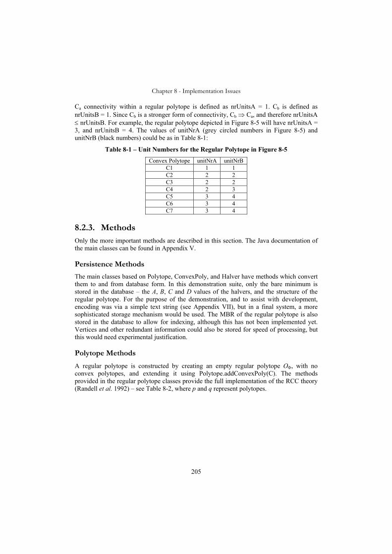
Chapter 8 - Implementation Issues
205
Ca connectivity within a regular polytope is defined as nrUnitsA = 1. Cb is defined as nrUnitsB = 1. Since Cb is a stronger form of connectivity, Cb ⇒ Ca, and therefore nrUnitsA ≤ nrUnitsB. For example, the regular polytope depicted in Figure 8-5 will have nrUnitsA = 3, and nrUnitsB = 4. The values of unitNrA (grey circled numbers in Figure 8-5) and unitNrB (black numbers) could be as in Table 8-1:
Table 8-1 – Unit Numbers for the Regular Polytope in Figure 8-5
Convex Polytope unitNrA unitNrB C1 1 1 C2 2 2 C3 2 2 C4 2 3 C5 3 4 C6 3 4 C7 3 4
8.2.3. Methods Only the more important methods are described in this section. The Java documentation of the main classes can be found in Appendix V.
Persistence Methods
The main classes based on Polytope, ConvexPoly, and Halver have methods which convert them to and from database form. In this demonstration suite, only the bare minimum is stored in the database – the A, B, C and D values of the halvers, and the structure of the regular polytope. For the purpose of the demonstration, and to assist with development, encoding was via a simple text string (see Appendix VII), but in a final system, a more sophisticated storage mechanism would be used. The MBR of the regular polytope is also stored in the database to allow for indexing, although this has not been implemented yet. Vertices and other redundant information could also be stored for speed of processing, but this would need experimental justification.
Polytope Methods
A regular polytope is constructed by creating an empty regular polytope OΦ, with no convex polytopes, and extending it using Polytope.addConvexPoly(C). The methods provided in the regular polytope classes provide the full implementation of the RCC theory (Randell et al. 1992) – see Table 8-2, where p and q represent polytopes.

Chapter 8 - Implementation Issues
206
Table 8-2 Implementation of the Basic Predicates of RCC theory
Operation Description Implementation
Ca(p, q) p is weakly connected to q
p.connectsToA(q)
Cb(p, q) p is strongly connected to q
p.connectsToB(q)
DCa(p, q) p is not weakly connected to q
¬p.connectsToA(q)
DCb(p, q) p is not strongly connected to q
¬p.connectsToB(q)
P(p, q) p ⊆ q p.isWithin(q)
PP(p, q) p ⊂ q p.properPartOf(q)
EQ(p, q) p = q p.equals(q)
OV(p, q) p ∩ q ≠ Oϕ p.intersects(q)
ECa(p, q) ),(OV),(Ca qpqp ¬∧
p.externallyConnectedToA(q)
ECb(p, q) ),(OV),(Cb qpqp ¬∧
p.externallyConnectedToB(q)
TPPa(p, q) ),(Ca qpqp ∧⊂ p.tangentialProperPartOfA(q)
TPPb(p, q) ),(Cb qpqp ∧⊂ p.tangentialProperPartOfB(q)
NTPPa(p, q) ),(Ca qpqp ¬∧⊂ p.nonTangentialProperPartOfA(q)
NTPPb(p, q) ),(Cb qpqp ¬∧⊂ p.nonTangentialProperPartOfB(q)
PO(p, q) p ∩ q ≠ Oϕ, p⊄q, q⊄p, p≠q
p.properOverlap(q)
Note that by RCC theory, all of these relations can be generated from the "connects" relation. In practice, some are directly calculated (such as “intersects” – for reasons as given in Section 6.2), but most are simply implemented as their definition suggests.
For example, the isWithin predicate:
/** Determines if this regular polytope is within the other * @param other The other regular polytope * @return True if this regular polytope is within the other */ public boolean isWithin(Polytope other) { Polytope otherM = other.inverse(); otherM = otherM.intersection(this); return (otherM.convexPolys.size() == 0); }

Chapter 8 - Implementation Issues
207
and the equals predicate:
/** Determines if this regular polytope is equal to the other * @param other The other regular polytope * @return True if every point in this regular polytope is * within the other and vice versa. */ public boolean equals(Polytope other) { return (this.isWithin(other) && other.isWithin(this)); }
The additional predicates p.isConnectedA() and p.isConnectedB() are provided to determine the internal connectivity of the regular polytope.
Table 8-3 Topological Functions on Regular Polytopes
Function Description Implementation
Complement ¬p p.inverse()
Union p ∪ q p.union(q)
Intersection p ∩ q p.intersection(q)
The basic functions of regular polytopes that return a regular polytope as a result are implemented as designated in Table 8-3.
In the demonstration software there is no provision for updating or modifying a regular polytope, convex polytope or halver in memory. For example, there is no provision to remove a convex polytope from a regular polytope, or to adjust the A, B, C, D of a half space. All such modification is accomplished by creating a new regular polytope as the result of operations between existing ones, or by creating and assembling new objects using basic constructors. This is not seen as a restriction, and any practical implementation would probably use this approach.
8.3. Proof of Concept Data Approximately one thousand parcels were selected from the Queensland Cadastre. The area chosen was the region surrounding the “Gabba” cricket grounds in Woolloongabba Brisbane, because this area contains some 3D parcels of non-trivial shape (Thompson 2005b). The parcels obtained from the database are 2D only, but do include secondary interests (such as easements). Thus overlapping 2D areas exist. There were several 3D parcels in the region. Two associated with the cricket stadium, and one with a restaurant were hand encoded.
In the original data, some inaccuracies had been introduced in the past through rounding, so there are slight overlaps and mismatches between the edges which have not been corrected. This will be discussed further in Section 8.6.

Chapter 8 - Implementation Issues
208
Figure 8-6 Overview of the test region.
8.3.1. Presentation of Regular Polytopes Figure 8-6 shows the data in question. The 2D parcels have been represented by colouring a plane (at z = 0) with a randomly selected colour. To further show the division between parcels, a vertical “fence” of the same colour has been drawn. Since the colour of the parcel on each side of the fence is different, some interfering visualisation effects can occur. The algorithm to convert from conventional polygon to regular polytope used a scan-line approach, from north to south. Each time a concavity is detected, a convex polytope is generated, and the scan continues. This is far from optimal, and there is scope for considerable improvement in this algorithm (see Section 10.2.6).

Chapter 8 - Implementation Issues
209
Figure 8-7 Detail of two 3D parcels (red and green) with a third (blue) in the
background. The vertical grey cylinder indicates the Z axis.
Figure 8-7 shows a detail of some of the 3D parcels (which abut without overlapping). (See also (Stoter 2004) pages 269-272 for a view of these same parcels. The encoding used in the red parcel is shown in Appendix VI Figure VI-3.
Figure 8-8 3D parcel amongst 2D parcels. (Parcel A and 2D parcel E together
comprise a restaurant. Parcel A overhangs the roadway represented by parcels B, C and D).
Figure 8-8 depicts a 3D parcel A overhanging the roadway, and exactly abutting the 2D parcel E directly below the open space partially enclosed by it.
AB
C
D
E
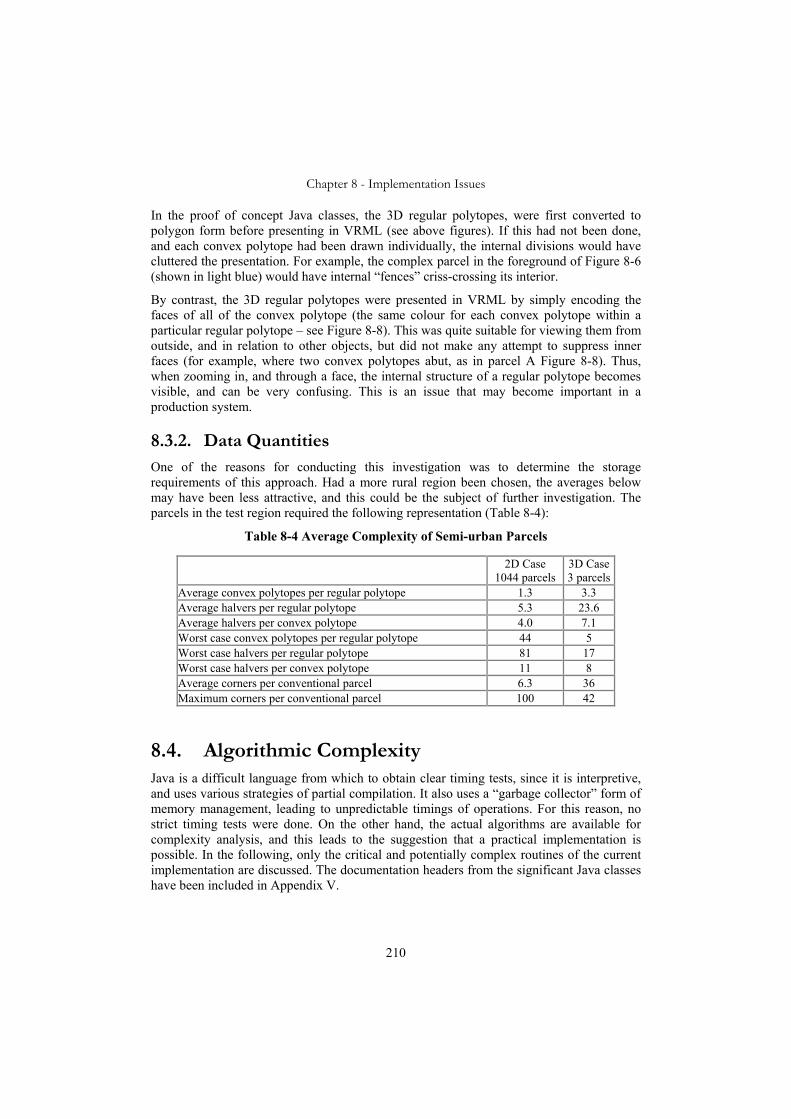
Chapter 8 - Implementation Issues
210
In the proof of concept Java classes, the 3D regular polytopes, were first converted to polygon form before presenting in VRML (see above figures). If this had not been done, and each convex polytope had been drawn individually, the internal divisions would have cluttered the presentation. For example, the complex parcel in the foreground of Figure 8-6 (shown in light blue) would have internal “fences” criss-crossing its interior.
By contrast, the 3D regular polytopes were presented in VRML by simply encoding the faces of all of the convex polytope (the same colour for each convex polytope within a particular regular polytope – see Figure 8-8). This was quite suitable for viewing them from outside, and in relation to other objects, but did not make any attempt to suppress inner faces (for example, where two convex polytopes abut, as in parcel A Figure 8-8). Thus, when zooming in, and through a face, the internal structure of a regular polytope becomes visible, and can be very confusing. This is an issue that may become important in a production system.
8.3.2. Data Quantities One of the reasons for conducting this investigation was to determine the storage requirements of this approach. Had a more rural region been chosen, the averages below may have been less attractive, and this could be the subject of further investigation. The parcels in the test region required the following representation (Table 8-4):
Table 8-4 Average Complexity of Semi-urban Parcels
2D Case 1044 parcels
3D Case 3 parcels
Average convex polytopes per regular polytope 1.3 3.3 Average halvers per regular polytope 5.3 23.6 Average halvers per convex polytope 4.0 7.1 Worst case convex polytopes per regular polytope 44 5 Worst case halvers per regular polytope 81 17 Worst case halvers per convex polytope 11 8 Average corners per conventional parcel 6.3 36 Maximum corners per conventional parcel 100 42
8.4. Algorithmic Complexity Java is a difficult language from which to obtain clear timing tests, since it is interpretive, and uses various strategies of partial compilation. It also uses a “garbage collector” form of memory management, leading to unpredictable timings of operations. For this reason, no strict timing tests were done. On the other hand, the actual algorithms are available for complexity analysis, and this leads to the suggestion that a practical implementation is possible. In the following, only the critical and potentially complex routines of the current implementation are discussed. The documentation headers from the significant Java classes have been included in Appendix V.
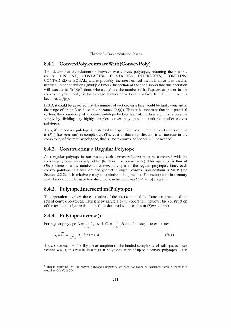
Chapter 8 - Implementation Issues
211
8.4.1. ConvexPoly.compareWith(ConvexPoly) This determines the relationship between two convex polytopes, returning the possible results: DISJOINT, CONTACTSa, CONTACTSb, INTERSECTS, CONTAINS, CONTAINED or EQUAL, and is probably the most critical method, since it is used in nearly all other operations (multiple times). Inspection of the code shows that this operation will execute in O(f1f2p2) time, where f1, f2 are the number of half spaces or planes in the convex polytope, and p is the average number of vertices in a face. In 2D, p = 2, so this becomes O(f1f2).
In 3D, it could be expected that the number of vertices on a face would be fairly constant in the range of about 3 to 6, so this becomes O(f1f2). Thus it is important that in a practical system, the complexity of a convex polytope be kept limited. Fortunately, this is possible simply by dividing any highly complex convex polytopes into multiple smaller convex polytopes.
Thus, if the convex polytope is restricted to a specified maximum complexity, this routine is O(1) (i.e. constant) in complexity. (The cost of this simplification is an increase in the complexity of the regular polytope, that is, more convex polytopes will be needed).
8.4.2. Constructing a Regular Polytope As a regular polytope is constructed, each convex polytope must be compared with the convex polytopes previously added (to determine connectivity). This operation is thus of O(n2) where n is the number of convex polytopes in the regular polytope1. Since each convex polytope is a well defined geometric object, convex, and contains a MBR (see Section 8.2.2), it is relatively easy to optimise this operation. For example an in-memory spatial index could be used to reduce the search-time from O(n2) to O(n log n).
8.4.3. Polytope.intersection(Polytope) This operation involves the calculation of the intersection of the Cartesian product of the sets of convex polytopes. Thus it is by nature a O(nm) operation, however the construction of the resultant polytope from this Cartesian product raises this to O(nm log nm).
8.4.4. Polytope.inverse()
For regular polytope iniCO
..1== U , with j
mji HC
i..1== I the first step is to calculate:
jmj
ii HCOi..1=
== U for i = i..n. (f8.1)
Thus, since each mi ≤ c (by the assumption of the limited complexity of half spaces – see Section 8.4.1), this results in n regular polytopes, each of up to c convex polytopes. Each
1 This is assuming that the convex polytope complexity has been controlled as described above. Otherwise it would be O(n2f2) in 3D.

Chapter 8 - Implementation Issues
212
convex polytope consists of one half space only. Thus, this first part of the operation is O(nc) = O(n) (because c is constant). Note that the inverse of a convex polytope consists of a regular polytope with up to c convex polytopes, each defined by one half space (see Figure 4-4 Chapter 4).
The second phase consists of forming the intersection of the n regular polytopes
iniOO
..1== I . If approached without any optimisation, this would be disastrous – leading to
an operation of order cn. Fortunately, the algorithm can avoid this. It proceeds as:
let R = O1; (f8.2) for i = 2..n, let R = R ∩ Oi; (f8.3)
At each step in the algorithm, a large number of convex polytopes that are generated by the intersection operation are discarded. At the end of the process, assume there are l convex polytopes left. If it is assumed that the number of convex polytopes in R remains fairly constant during the process, this means that the cost of each operation at f8.3 will be O(l log l). Since there are n operations, this gives O(nl log l). Note that l in this formula, like n is the measure of the complexity of a single regular polytope. Nevertheless, this is an algorithm which could well repay some optimisation effort beyond the simple version used in the demonstration software.
8.4.5. Other Regular Polytope Operations All of the other regular polytope operations (as shown in Tables 8.1, 8.2 and 8.3) are simple combinations of other operations (e.g. see Section 8.2.3). So that the worst cases will be of no higher complexity than Polytope.inverse or Polytope.intersection – that is O(n2 log n), where n is a representative size of a single regular polytope in terms of the number of convex polytopes.
8.4.6. Indexing and Searches The programs as developed as a proof of concept do not yet use any database spatial indexing, and so are not efficient for doing spatial searches. On the other hand, they do generate a minimum bounding rectangle (or solid) with approximated X, Y and Z integer values surrounding the vertices of each regular polytope and each convex polytope, and so a standard R-Tree algorithm can be used.
8.4.7. BigInteger Arithmetic One of the advantages of implementing these routines in Java was the availability of the BigInteger object class. This makes available a complete set of arithmetical operations on an integer representation with (effectively) no limit on the size of operands. The disadvantage of BigInteger is the slow speed of the operations, and the fact that the speed of operations is dependent on the size of the numbers involved.
In order to implement this software in a language other than Java (e.g. C), some of this functionality will need to be implemented, but fortunately not all. It is not necessary to allow for potentially infinite operands – although large numbers are involved, they are

Chapter 8 - Implementation Issues
213
constrained. (In order to give millimetre precision in a region the size of Queensland, 96 bit integers are needed in 2D and 160 bit integers in 3D). Further, not all arithmetic operations need be implemented – negation, addition and multiplication are needed, but division is not (this is a considerable simplification). An approximation of a BigInteger as a double precision floating point number is also needed for display and conversion purposes.
8.4.8. Java Code Tuning The use of more appropriate implementations of the collection class in the Java code could lead to a very easy speed improvement. In the demonstration system, the "Vector" class was used for all collections of objects rather than the most appropriate class. In some cases, this will have caused a significant speed reduction - since, for example, the "insert" operation on a vector is of O(n) where n is the current number of objects in the vector – a linked list in a similar operation is of O(1). The reason for this inappropriate use of vector was simply that it is much easier to view the contents of a vector in debug mode.
8.5. Optimising the Model Optimising techniques would benefit from control of the complexity of the individual convex polytopes. The calculation of the vertices of a convex polytope is a significant process, strongly dependent on the cardinality of the set of half-spaces in a convex polytope. Restricting this cardinality as shown in Figure 8-9 can control this complexity, even at the cost of increasing the cardinality of the set of convex polytopes in a regular polytope.
c is a chosen limit on the cardinality of the relation
RegularPolytope
ConvexPolytope 0:*
1:* HalfSpace
A, B, C, D
Regular Polytope
RegularPolytope
ConvexPolytope 0:*
1:c HalfSpace
A, B, C, D
Regular Polytope
Figure 8-9 Left - general regular polytope, right – limited convex polytope form.
For example, in Figure 8-10, assuming that regular polytope O1 has been split into four complex polytopes just to simplify the convex polytopes that comprise it, the split can be carried out in such a way as to improve the selectiveness of the MBR’s of the convex

Chapter 8 - Implementation Issues
214
polytopes. Thus the operation of forming the union or intersection of O1 and O2 is much more efficient, since it is clear that C1, C2 and C3 are disjoint from O2.
C1 C2 C3 C4 O2
O1
Figure 8-10 Union of regular polytopes O1 and O2.
It is significantly easier to optimise the operations between convex polytopes, for example, by using an in-memory spatial index to eliminate cases where two convex polytopes cannot intersect (see Section 8.4.2).
While not necessary in the theory, it may improve the efficiency of many operations if the disjoint normal form (DNF) (see Section 4.1.5) is used in representing regular polytopes. In this form, the convex polytopes that comprise a regular polytope are mutually disjoint – so that all overlaps between convex polytopes are replaced by Cb connectivity. There are two advantages to this form:
• It is far easier to calculate the volume of a regular polytope already in DNF.
• The indexing and comparison of convex polytopes can be improved, since the disjoint convex polytopes will have smaller minimum bounding rectangles.
The only disadvantage is that on initial data uptake, and following certain operations (in particular union and complement) the disjoint form must be generated. A sketch of the algorithm to convert a regular polytope to DNF can be found in Section 4.1.5.
A2
A1
B
Figure 8-11 Calculating the intersection of two regular polytopes.

Chapter 8 - Implementation Issues
215
In calculating the intersection of region B with region A in Figure 8-11 (shown above split into two convex polytopes A1 and A2), even though all the half planes which define A1 intersect all the half planes that define B (since they are not parallel, and the half plane definition is theoretically infinite), it can be determined by a conventional polygon overlap test that all the vertices of A1 are completely separated from the vertices of B – therefore A1∩B is empty. This kind of logic can be used to pre-eliminate large numbers of the partial intersections, and could be augmented by an in-memory spatial index – e.g. an R-Tree based on the minimum bounding rectangles (shown as dashed lines) to further improve the calculation speed.
8.5.1. Optimisation of Convex Polytope Shapes. In 3D, it might be considered that a regular polytope representation based on tetrahedral convex polytopes (or triangular in 2D) would be particularly useful. A tetrahedron fulfils the requirements of a convex polytope, and various algorithms exist to “tetrahedronise” a general polyhedron (or triangulate a polygon). These techniques have been extensively studied, and optimised for various criteria.
Unfortunately, while it is quite possible to define tetrahedral convex polytopes a tetrahedral decomposition is not possible in general. Consider the intersection of two triangular convex polytopes as in Figure 8-12. (Using a 2D example for simplicity of depiction). In general, this will result in a null region or a convex polytope with 3, 4, 5 or 6 sides. For closure of the representation, it would be necessary to split this into triangles.
Figure 8-12 Two triangular regions with a hexagonal intersection.
To split a convex polytope into triangular regions, it would be necessary to construct pairs of half planes that divide the region at the existing vertices. This is equivalent to determining integer values A,B and D such that
Ax1+By1+D = 0 and Ax2+By2+D = 0 for dr-rational numbers x1, y1, x2 and y2.
These integers can always be found, but the requirements that –M < A,B < M, -2M2 < D < 2M2 (in 2D) cannot be guaranteed. Thus, as can be seen in Figure 8-13, it is not possible in this way to guarantee to divide a region into triangles. If the dividing line cannot be

Chapter 8 - Implementation Issues
216
guaranteed to pass through two vertices, a pentagon can only be divided into a quadrilateral and a pentagon. (Note that the region on the left after the division still has 5 sides). This is not to say that the regular polytope cannot be used to represent a land surface (for example), but that such a representation will not be based on a triangulation, or will have small overlaps at the junction of regions.
Figure 8-13 Attempting to divide a pentagon.
8.6. Data Load Issues In the proof of concept programs, a conversion routine was developed to transform polygons into 2D regular polytopes. The routine as developed was not ideal. Using a scan-line approach, it has a strong tendency to generate convex polytopes that are extended in an east-west direction. This militates against efficient processing later, since badly formed bounding rectangles result. Although as discussed in Section 8.5.1, it is not possible in general to maintain a triangular or tetrahedral convex polytope decomposition within the domain restriction, this approach will still be useful in the optimal conversion of polyhedra into regular polytopes. There are techniques available (Garey et al. 1977; Narkhede and Manocha 2004) to decompose a polygon into triangles, with various criteria for evaluating the decomposition. Variants of these routines can operate in 3D.
It seems likely that there is an optimum number of half spaces per convex polytope, balanced against the decomposition of regular polytopes into convex polytopes, and that an algorithm that first decomposes the polyhedra, and then selectively recombines them based on certain criteria may lead to this result.
A major issue in the conversion of existing data into regular polytope form is the lineage of that data. Once the geometry is expressed in regular polytope form the operations between geometric regions are guaranteed to be rigorously correct, but the quality of the source data must be considered. Approximations may well have been made, and inaccuracies introduced to allow the data to be stored in the previous form, and this may create difficulties in data uptake.

Chapter 8 - Implementation Issues
217
8.6.1. Introduced Inaccuracy In many systems, calculation of the point of intersection between lines introduces rounding errors as in the circled points on the road frontage in Figure 8-14, which was intended to be a straight line connecting A and B. In addition, to avoid later topological failures – as described in Case 6 – Chapter 2, a further displacement of the calculated point is often applied, as pictured in Figure 8-15.
A
B
Figure 8-14 Points moved slightly in the calculation of intersections (shown
exaggerated).
This assumes that the data is to be loaded from an existing spatial database. In some cases, it may be possible to capture from the original source – e.g. the survey data. Unfortunately, while it would have been ideal to have captured original data in its uncompromised form, this is rarely the case, and much processing has been done to data before it reached the database. For example, bearings and distances will have been adjusted to “close”, elevations of 3D points will have been calculated from the raw field notes, horizontal displacements will have been calculated from slope distances, etc. Note that there is a trend in which the original observations and measurements are more often stored in the (cadastral) database, in addition to the resulting interpretations (parcels) (Tarbit and Thompson 2006).
A
B
C
E
p
q
l
Figure 8-15 Polygon point q has been inserted into line l.
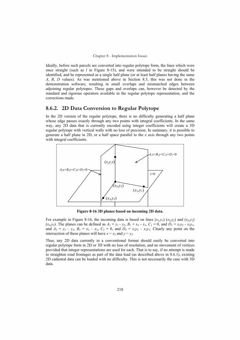
Chapter 8 - Implementation Issues
218
Ideally, before such parcels are converted into regular polytope form, the lines which were once straight (such as l in Figure 8-15), and were intended to be straight should be identified, and be represented as a single half plane (or at least half planes having the same A, B, D values). As was mentioned above in Section 8.3, this was not done in the demonstration software, resulting in small overlaps and mismatched edges between adjoining regular polytopes. These gaps and overlaps can, however be detected by the standard and rigorous operators available in the regular polytope representation, and the corrections made.
8.6.2. 2D Data Conversion to Regular Polytope In the 2D version of the regular polytope, there is no difficulty generating a half plane whose edge passes exactly through any two points with integral coefficients. In the same way, any 2D data that is currently encoded using integer coefficients will create a 3D regular polytope with vertical walls with no loss of precision. In summary, it is possible to generate a half plane in 2D, or a half space parallel to the z axis through any two points with integral coefficients.
(x1,y1) (x2,y2)
(x3,y3)
(x4,y4)
(x,y,z)
z=0
A1x+B1y+C1z+D1=0
A2x+B2y+C2z+D2=0
Figure 8-16 3D planes based on incoming 2D data.
For example in Figure 8-16, the incoming data is based on lines (x1,y1) (x2,y2) and (x2,y2) (x3,y3). The planes can be defined as A1 = y1 - y2, B1 = x2 - x1, C1 = 0, and D1 = x1y2 - x2y1, and A2 = y3 – y2, B2 = x2 – x3, C2 = 0, and D2 = x3y2 – x2y3. Clearly any point on the intersection of these planes will have x = x2 and y = y2.
Thus, any 2D data currently in a conventional format should easily be converted into regular polytope form in 2D or 3D with no loss of resolution, and no movement of vertices provided that integer representations are used for each. That is to say, if no attempt is made to straighten road frontages as part of the data load (as described above in 8.6.1), existing 2D cadastral data can be loaded with no difficulty. This is not necessarily the case with 3D data.

Chapter 8 - Implementation Issues
219
8.6.3. 3D Data Conversion to Regular Polytope Where 3D data is to be converted to regular polytope form, some care is needed. In contrast to the 2D case where a half plane can be guaranteed to pass through any two integral co-efficient points, the best that can be asserted in 3D is that a half space can be generated whose boundary plane passes within one grid1 unit of resolution of each of the points. In many special cases – specifically where the half space is parallel to any of the axes – much better results can be expected, but the worst case is one unit error. If a situation such as that of Figure 8-15 occurs in a 3D situation, and the bend at point q is straightened, the actual position of point p (as a point of intersection) is subject to a large variation.
A
B
C
E
p
q
Figure 8-17 Imprecision in the placement of the point of intersection. (This diagram
should be interpreted as a slice through a 3D situation).
In Figure 8-17, where the half spaces that define region E have a possible imprecision of one unit, their line of intersection at p has a much larger possible error (shaded). If this is a critical issue, it may be solved by introducing a deliberate bias to the approximation, and an additional half space to limit the position of p. The bias is needed to extend the convex polytope because the addition of a half plane will not be effective if it is redundant to the convex polytope definition.
new half plane
A
B
C
E
p
q
Figure 8-18 Half space introduced to constrain the point position.

Chapter 8 - Implementation Issues
220
For example, in Figure 8-18, the boundary of region E has been extended (still within one unit of resolution), and the acute angle at point p has been truncated. This procedure – of truncating any acute dihedral angles – could be used as a general procedure in converting geometric objects into regular polytope form where the point or line of intersection is known, and must be maintained. Note that objects with very acute angles have many unfortunate and unexpected properties in any geometric representation (see also Section 6.8.3). It is common for objects with very acute angles to be the subject of validation on data uptake, since such angles are often the result of mistakes or inaccuracies in data capture.
8.7. Conclusions The regular polytope approach is shown to be practical, and could be rigorously implemented as a large-scale database (with proven functionality and without unpleasant surprises due to the mismatch of infinite real number mathematics and the finite digital computer). While some more optimisation in the area of the regular polytope algorithms could yield speed improvements; for at least the sort of data used in this pilot system, acceptable results were obtained. In the test region, it was possible to run any combination of the standard RCC and topological functions, and the combination and nesting of functions gave completely predictable results. The indication is that a full implementation could be developed with query and analysis, and edit/update functionality.
It is expected that, as described above, restricting the complexity of convex polytopes will lead to practical speeds. In the case of 2D polytopes, several thousand half planes per complex polytope should be practicable. In 3D, the number is probably several hundred. This is appropriate particularly for cadastral data, whereas the parcels with large numbers of points (more than 2000) required in their definitions generally occur in rural areas, and are all 2D. Otherwise, complex convex polytopes can be artificially subdivided into a number of simpler convex polytopes.
The overwhelming advantage of the regular polytope approach is in the rigorously correct logic that it supports, and this justifies some additional data storage requirements (see Appendix VII and Chapter 7), and the potentially slower processing times, but there is still much potential to improve the implementation of some of the operations – in particular, Polytope.intersection(), and Polytope.inverse().
The next chapter reviews the case studies that were introduced in Chapter 2, in light of the findings that have been presented in this thesis, and the functionality of the regular polytope representation.

Chapter 9
Review of Case Studies
The preceding chapters have defined the regular polytope representation, and have explored its functionality and expressivity. This chapter reviews the specific cases that were cited in Chapter 2 as showing common deficiencies in current systems in light of their solutions using the regular polytope. Each case is directly referred to the corresponding section in Chapter 2.
9.1. Case 1. Polygon Union In the regular polytope representation, it has been shown in Appendix II.11 (see also Section 4.1.4) that all the operations that have been implemented are mathematically rigorous. Thus, for example, the union operation is associative i.e.
CBACBA ∪∪=∪∪ )()( . In general, the result of calculation of ini
A..1=U cannot depend on
the order of execution.
9.2. Case 2. Data Interchange If spatial features are encoded and interchanged in a form such as that used in the demonstration software, and defined in Appendix VII, the regular polytopes will arrive in an identical form, with no loss of resolution, and clearly with no change to the topology of the regions. This is not, however, a complete answer, since it must be possible to transfer features between systems with different available resolutions. For example, if the A,B and C values are stored as 32 bit integers, and the D as 64 bit, it may be necessary to transmit
Chapter 9 – Review of Case Studies
222
the features to a system that uses smaller integer representations (for example 16 and 32 bits respectively).
Any reduction in the available resolution will potentially result in loss of precision, and so this will by nature be a so-called "lossy" transmission. One possible approach to this is to use a rounded floating point "normalised" transmission strategy.
Such a strategy could be as follows: Operating in floating point arithmetic, a, b, c, and d are calculated as A, B, C and D, divided by 222 CBA ++ . Thus, -1 ≤ a, b, c ≤ 1. It may
be necessary to use extended precision floating point to calculate 222 CBADd
++= . These
numbers are then rounded to an appropriate number p of decimal places for transmission and converted to integer by multiplying by p10 . Provided the floating point operations are sufficiently accurate, the result will be that all of the parameters will on arrival have been perturbed by some small amount (less than p−10 in relative terms).
On arrival, after a “lossy” transmission, the geometry will certainly have changed slightly, but will still be valid – since any possible intersection of half spaces is a valid convex polytope, and any union of convex polytopes is valid as a regular polytope. There is the possibility that a previously connected regular polytope could become not connected on arrival, and it is possible that a convex polytope could become empty in transmission (see also Case 4 Section 2.4) It is also possible that a half space could become redundant to the definition of a convex polytope.
The robustness approach described in Section 5.7 is indicated where lossy transmission or reduction in resolution is needed, but it must be remembered that even in the event of fragile convex polytopes and fragile connectivity, a regular polytope cannot become invalid due to perturbation.
9.3. Case 3. ISO 19107 Definition of equals() The definition of equals as developed in this research has been shown for the dr-rational interpretation (in Chapter 4) to be a true equivalence relation, and that:
EQ(O1,O2) ⇔ (∀p, p∈O1 ⇔ p∈O2) (i.e. EQ is equivalent to point-set equality).
This means that issues such as the failure of transitivity exhibited in this case study cannot occur.
It is clearly still possible to define an "approximately equal" test, allowing a tolerance, and an "identically equal" test to determine that the representation is the same (see Case 13 Section 9.13).

Chapter 9 – Review of Case Studies
223
9.4. Case 4. ISO 19107 Definition of isSimple() There is no need for a test of this kind in the regular polytope representation. The representation is sufficiently robust to ensure that small knots will not cause breakdown of the software. There may still be a need to detect and warn of small convex polytopes, and cases of weak connectivity within a regular polytope, in order to detect data capture deficiencies. For example, in many problem domains (for example, cadastre), if a regular polytope is not robustly internally connected (see Section 5.7), or contains non-robust convex polytopes, it is likely that a data capture error has occurred. In contrast to the vertex representation cases, this is not needed to ensure correct processing, but is only to attempt to correct encoding errors.
vertex representation polytope representation
a
b
c
Figure 9-1 Non-simple and weakly connected geometries represented as polytopes.
Referring to Figure 9-1, cases such as a, (sometimes known as a "butterfly polygon") must be corrected by the conversion to regular polytope form, since the half spaces that define a convex polytope have a specific inside. Figure 9-1 Case b, where a small knot is in the positive, anticlockwise direction, a separate weakly connected convex polytope is generated. If this is extremely small, it may be preferable for it to be either discarded, or flagged for manual investigation. Figure 9-1 Case c, where the boundary lines of the original polygon do not cross would not be detected as a failure of the isSimple() test. As a regular polytope, it would be represented as the union of two convex polytopes, which are Cb connected (since they meet at more than a single point). Nevertheless, this is a situation that should be brought to a data custodian’s attention, because the connection is not robust (see Section 5.7). A small perturbation of the half spaces that define the region could easily change the Cb connection to Ca or no connection at all. The approach of Section 5.7 allows a robustness parameter to be assigned as suggested by Thompson and van Oosterom (2006a).

Chapter 9 – Review of Case Studies
224
9.5. Case 5. Intersection of a Point with a Line The regular polytope representation, in common with the dual grid approach, ensures that every possible point of intersection of two lines (in 2D), or three planes (in 3D) is representable as a point on the second level of resolution (grid2) (see Section 4.4.2), provided that the rules for the definition of the lines/planes are followed.
In the case of the approximated polytope, and the topologically encoded representations, a reduced accuracy representation of the dr-rational points is also stored. This semi-redundant storage is linked within the data model in a way analogous to the ISO19107 "interior to" (see also Section 2.8). These reduced accuracy points are useful in the calculation of approximate volumes, surface areas, distance between features etc., and can be used for first pass indexing operations (for example, they can be used to show that a feature definitely does not intersect a search region). They should not, however, be used to define actual half spaces, in the process of defining new regular polytopes, unless it is recognised that this is an approximation process.
9.6. Case 6. Narrow Cadastral Parcels
A
B
C
E
p q
r s
Figure 9-2 Narrow cadastral parcel and adjoiners.
This case is stated in 2D, and is simply handled using the regular polytope approach, since it is possible to generate a half plane whose edge passes exactly through points p and r, and one through p and s. If the non-topologically encoded form of regular polytope is being used to represent a collection of regions such as depicted in Figure 9-2 (reproduced from Figure 2-11) (with no adjacency information compiled into the database), each region can be represented adequately by a single regular polytope. The only potential problem is that region E has a non-robust Cb connection to C, and so the connectivity may be broken by any small perturbation of the definitions. The definitions would still be valid after perturbation in all cases, but connectivity could be lost. This situation could be detected, and a warning of non-robustness given at data uptake time in the same way as was

Chapter 9 – Review of Case Studies
225
described in the discussion of Case 4. If the objects were being stored in a topologically encoded form, as described in Section 7.3, the lines pq and qr would be represented by a single half space record.
9.7. Case 7. 3D Surfaces and Lines The equivalent issues to the above in 3D are equally well handled in the regular polytope approach. Also, because all surfaces are built from half space definitions, no lack of planarity can be introduced by errors or imprecision in encoding. Since the 2D situation in the regular polytope representation is in effect seen as a special case of the 3D representation, there is no difficulty in carrying arguments into the 3D cases.
The only additional issue in the case of 3D data is that, while in 2D, a half space can be generated which exactly passes through two points which have integer coordinates, in 3D it can only be guaranteed that a half space (in the form described in this thesis) will pass within one grid1 unit of three given points. This means that there is an element of approximation involved in conversion from a vertex-based representation to a regular polytope representation.
9.8. Case 8. ISO 19107 Definition of "interior to" Association
The regular polytope representation does not have the concept of a line or a surface (in 3D) as a point set feature. Thus it is not meaningful to ask whether a point is interior to a line or surface. In addition, there is no concept of a boundary point set. The question of whether a point is “interior to” a regular polytope is rigorously answered.
In the case of the approximated polytope and the topologically encoded representations, a reduced accuracy representation of all vertices is stored. These are linked within the data model to their defining half spaces, and are asserted to be within a defined unit of resolution of all the half spaces that define them. This is analogous to the ISO19107 "interior to" association but the linkage is maintained in every case, not merely when there is a possibility of error. This only applies to the approximated points, and not to the basic regular polytope representation.
9.9. Case 9. Adjoining Polygon Points Using the basic non-topologically encoded regular polytope representation there is no need for any change to the definition of parcel A in Figure 9-3 (reproduced from Figure 2-13). The common boundary between A and B and the boundary between A and C will be exact, and have exactly the same parametric definition after the subdivision as before. Parcel A remains as a single convex polytope defined by four half planes.
In the topologically encoded representation of Section 7.3, a single half plane record defines the faces ap and pb (as part of the definition of C and B) and the face ba as part of

Chapter 9 – Review of Case Studies
226
the definition of A. This half plane would be encoded for example linked to convex polytopes B and C, and linked (as a complement) to convex polytope A. Thus the boundaries of A with B and C are by definition exactly co-planar. In the discrete model shown in Section 7.2, the parameters of the faces are stored separately on each face record, but programmed constraints can be introduced to ensure coverage as described in Section 5.6. This is a matter of detail in the data model, and the decision would depend on the detailed requirements of the application
A
B
C
p
a
b
Figure 9-3 Subdivision of adjoining parcel.
9.10. Case 10. 3D Cadastre Issues The equivalent problem in 3D has exactly the same solution in the regular polytope representation as the 2D problem.
z
x
1 3
2a
2b
2d p q
t u
2c r s
Figure 9-4 Volumetric parcels adjoined by normal (2D) parcels, viewed from the side.
Figure 9-4 represents a vertical slice (side view) of a section of the cadastre (reproduced from Figure 2-14). In any of the regular polytope data models discussed in Chapter 7, the parcels 1 and 3 can be represented as simple prisms with no top or bottom, and with no

Chapter 9 – Review of Case Studies
227
reference to the edges p, q, r, s, t, u. Parcels 2a to 2d only differ in having one or two horizontal half spaces in their definition. The models which use shared half space topology are particularly suited to this type of situation.
9.11. Case 11. Datum Conversion The process of a change of datum will require calculation and rounding of the parameters of the half spaces that define the regular polytopes. As such, the issues discussed in Case 2 and Case 4 above apply. In addition, there is a further factor to be considered. A datum change will involve the shifting of coordinate values by differing amounts in different parts of the region of interest, and in theory at least, the bending of previously straight lines. Thus there will be localized stretching, rotation, and warping of the geometry. In the vertex based representations, it is usual to re-calculate the positions of the vertices, and simply assume that the lines or surfaces joining them remain straight. This is usually a good enough approximation, and the same approach can be used in the regular polytope representation1.
In effect, the approximate vertices are calculated, and the datum change is applied to them. The deltas of this movement are then converted back into changes in the parameters (A, B, C and D) of the half spaces. It is possible that two half spaces with the same parameters, but defining regions which are far apart, may become unequal as a result of this operation (if the amount of movement in each area is different).
9.12. Case 12. Uniqueness Of Representation The rigorous definition of the test for equality means that this is not an issue. It is common for regular polytopes to have different possible representations, but to be equal.
9.13. Case 13. GeoTools/GeoAPI definition of Object.equals()
As described in Section 2.13, a calculated hash code is used by various collection structures in Java to provide fast access to members. The function hashCode must generate a key value such that:
a.equals(b) ⇒ hashCode(a) = hashCode(b) (f8.1) ¬ a.equals(b) <nearly always implies> hashCode(a) ≠ hashCode(b) (f8.2)
The “nearly always implies” determines how useful the hashCode algorithm is. It should be relatively rare that two unequal objects have the same hash code.
1 Where this approximation is not acceptable: in the case of long straight lines, or regions of large relative distortion, as in the case of vertex representations, it will be necessary to re-calculate the representation.

Chapter 9 – Review of Case Studies
228
There are practical reasons for providing an "equals" test which is more restrictive than the equality operation EQ(A, B) defined in Section 4.2.5. Consider a database, in which updated objects are to be posted back to the database, but only if they have been changed (where the pre-image is unequal to the post image). If a regular polytope is extracted and changed so that its representation is changed, but it is still equal to its earlier form (by the EQ operation), then the change will not be written back to the database. For example, a process that extracted regions, converted them to disjoint normal form, and then posted them back would surprise the operator by not making any changes. Thus “equals()” as required in the Java object class is a different concept from EQ – which is defined as point-set equality.
For this reason, it may be necessary to define a.equals(b) as requiring that the representation of a and b be identical in terms of the break up of a and b into convex polytopes, and in terms of the half space parameters used to define those convex polytopes. If this is the case, a simple hashCode() routine can be based on the critical parameters (e.g. hashing the A, B, C, D values of all half spaces in all convex polytopes).
If this consideration does not apply, and the point set definition of equals is desirable – where a.equals(b) ⇒ (∀p, p∈a ⇔ p∈b), then a compatible definition of hashCode() will be necessary. This will need to be based on the actual points, but could be something like a hash of the x,y,z coordinates of all of the external dr-rational vertices of the regular polytope. (Where an external vertex of a regular polytope is defined as any vertex of a convex polytope that is not within the pseudo-closure of any other convex polytope). Other more easily calculated hash routines could be proposed.
9.14. Conclusions The regular polytope representation has been shown to address many of the kinds of problem that exist in current software. The rigorous logic underpinning the representation ensures that the gross failures caused by apparently trivial rounding and calculation effects do not occur. This means that a toolkit of functions and predicates can be assembled, with a guarantee that they can be used and combined in any way without danger of failure.
This approach can also be used to define rigorously a set of validity and robustness criteria that will greatly assist the effort to make spatial data interchangeable.
The next chapter summarises this research, and suggests some further work that could be undertaken to complement and continue it.

Chapter 10
Conclusions
In the previous chapters, the regular polytope representation of spatial objects has been introduced, and its characteristics explored in some detail. The investigation has concentrated on the algebraic completeness of the approach, and the rigour that can be achieved, with particular attention having been placed on the question of connectivity. In the previous two chapters, practical issues of implementation were considered.
Chapter 1 introduced the main topic of this research, and defined the scope. Chapter 2 contained a selection of case studies that illustrated the problems that can be caused by breakdown of the internal logic of representations. Chapter 3 contained a review of existing approaches to the issue.
Chapter 4 defined the regular polytope and presented some of the basic topological behaviour of the approach. Chapter 5 continued this into the issue of connectivity, and Chapter 6 discussed the algebras that the representation supports.
Chapter 7 presented some alternative database schemas that could be developed, and Chapter 8 documented the set of “proof of concept” Java classes that were developed in the process of this research. Chapter 9 reviewed the case studies of Chapter 2 in light of the regular polytope representation.
This chapter summarises the findings in terms of the research question and the results obtained and discusses potential for further research. Section 10.1 discusses extension of the representation to geometric objects of lower dimensionality than that of the embedding space (for example, surfaces in a 3D world).
Section 10.2 summarises the findings of the research, with a particular emphasis on those topics that are potential subjects for further investigation, and finally Section 10.3 presents

Chapter 10 - Conclusions
230
the conclusions that can be drawn from this research, and the contribution that this research has made to the field of spatial data representation.
10.1. Application of the Regular Polytope to Lower Dimensionality
As defined in the earlier chapters, the regular polytope is restricted to the representation of regions of the same dimensionality as the spaces in which they are embedded – solids in a 3D space, area features in a 2D space. Before discussing the extension of the approach to lower dimension objects, it is important to consider what these objects are, and how they become an issue in a spatial database. There are two broad categories of lower dimensional objects, and each has its own issues in representation. An object can be represented at such a small scale that there is no value in recording its thickness or extent. For example, a road that is captured at a scale of 1:2,000,000 is adequately represented as a linear feature. Likewise a small town may be represented as a point.
The other broad class of lower dimensionality objects are the boundaries of higher dimensional objects, where these boundaries are to be stored as features in themselves, possibly because they carry their own attributes (e.g. quality, date of survey …). For example a state border is often stored as a linear feature, whereas in fact it is the boundary between two area features.
As discussed in Section 7.2 The regular polytope representation does permit the halver objects to carry individual attributes that do not apply to the volume of the convex or regular polytope as a whole.
10.1.1. Boundary Objects The discipline of Mereotopology treats a boundary as a special kind of object – to quote Smith (1997) "Boundaries of bodies are actual parts of the bodies which they bound. But they are not just any sort of part; rather they are parts which, as a matter of necessity, can exist only as proper parts of things of higher dimension which they are the boundaries of (where from the set-theoretical point of view, isolated extensionless points are presented as existing in complete independence of any larger wholes)".
There is not complete agreement on whether a boundary should be considered part of the object (as in the case of two billiard balls in contact – each having its own boundary), or a common object delineating the division between two objects (such as a state border). The mereological approach is that the boundary is a part of the object, but two boundaries can be defined by the same set of points. This is in contrast with the principle of topological encoding, where a boundary is treated as a single discrete object with a positive and a negative side, which links to and serves to define the two (or more) regions.
It may be that this dichotomy in the view of boundaries reflects the size of the object being considered – with hard edged boundaries being applicable to small objects (such as an
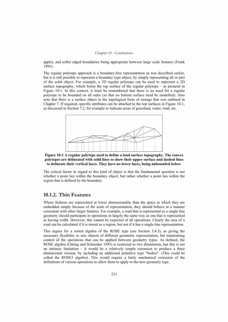
Chapter 10 - Conclusions
231
apple), and softer edged boundaries being appropriate between large scale features (Frank 1995).
The regular polytope approach is a boundary-free representation as was described earlier, but it is still possible to represent a boundary type object, by simply representing all or part of the solid object. For example, a 3D regular polytope can be used to represent a 2D surface topography, which forms the top surface of the regular polytope – as pictured in Figure 10-1. In this context, it must be remembered that there is no need for a regular polytope to be bounded on all sides (so that no bottom surface need be modelled). Also note that there is a surface object in the topological form of storage that was outlined in Chapter 7. If required, specific attributes can be attached to the top surfaces in Figure 10-1, as discussed in Section 7.2, for example to indicate areas of grassland, water, road, etc.
Figure 10-1 A regular polytope used to define a land surface topography. The convex polytopes are delineated with solid lines to show their upper surface and dashed lines to delineate their vertical faces. They have no lower faces, being unbounded below.
The critical factor in regard to this kind of object is that the fundamental question is not whether a point lies within the boundary object, but rather whether a point lies within the region that is defined by the boundary.
10.1.2. Thin Features Where features are represented at lower dimensionality than the space in which they are embedded simply because of the scale of representation, they should behave in a manner consistent with other larger features. For example, a road that is represented as a single line geometry should participate in operations in largely the same way as one that is represented as having width. However, this cannot be expected of all operations. Clearly the area of a road can be calculated if it is stored as a region, but not if it has a single-line representation.
This argues for a sorted algebra of the ROSE type (see Section 3.4.5), as giving the necessary flexibility to mix objects of different geometric representation, but maintaining control of the operations that can be applied between geometry types. As defined, the ROSE algebra (Güting and Schneider 1995) is restricted to two dimensions, but this is not an intrinsic limitation – it would be a relatively simple extension to produce a three dimensional version, by including an additional primitive type "bodies". (This could be called the ROSE3 algebra). This would require a fairly mechanical extension of the definitions of various operations to allow them to apply to the new geometry type.

Chapter 10 - Conclusions
232
The ROSE algebra has already been shown to be implementable using the realms approach (Güting et al. 1995), and by the dual grid approach (Lema and Güting 2002). As these are quite different forms of representation, this further argues for the flexibility of the ROSE algebra and its suitability to the extended regular polytope context.
10.1.3. Definition of Primitives It is not the intention to pursue this in great detail here, merely to indicate a possible line of further research based on the 3D dr-rational representation of regular polytopes. The 3D primitive has already been defined – the regular polytope itself.
The 2D convex primitive could be defined in 3D space as the dr-rational points p = (x,y,z) where Ax + By + Cz + D = 0. In the dr-rational representation, this is a finite set of points (as are all computer representations), but as described in Section 7.7.2, the set is “fairly dense”, containing a large number of dr-rational points. This is an unbounded plane, but if it is intersected with one or more half spaces Hi: i = 1..n, a partially or fully bounded "convex surface patch" can be defined. Surface patch P is defined by A, B, C & D and Hi: i = 1..n such that
p ∈ P if Ax + By + Cz + D = 0 and p ∈ Hi: i = 1..n.
Note that this is a point set, and that the set of half spaces can be viewed as a convex polytope {Hi: i = 1..n} (not necessarily explicitly fully bounded except by the “universal box” – see def4.13). That is to say, a convex surface patch is defined as the intersection of an unbounded plane with a convex polytope. The 2D primitive "surface" in 3D space can then be defined as the union of the points in a number of convex surface patches.
In a similar way, the 1D (convex) line segment could be defined as the points satisfying A1x+B1y+C1z+D1= 0 and A2x+B2y+C2z+D2= 0, delimited by a number of half spaces (two would be sufficient).
The 0D primitive could be defined using three equations, but more simply as a dr-rational point.
Ca would be defined as before as the existence of a point within the pseudo-closure of each primitive, while Cb would be defined as Cb(x, y) if a convex primitive z of the same dimension as either x or y can be found that is entirely within x∪y and x∩z is not empty and y∩z is not empty. (If x and y are solids, then z must be a solid. If a solid and a surface, then z would have to be a surface etc). As can be seen in Figure 10-2, this definition of Cb leads to rather unusual results. For example, the two regions of Case 7 by this definition would be Cb connected. For this reason it would be preferable instead to use the form of continuity defined by Clementini et al (1993), shown in Figure 10-2 as C0, C1 or C2 (or C3 = overlap) where the subscript defines the dimensionality of the overlap between the pseudo-closures of the regions.

Chapter 10 - Conclusions
233
Ca Cb ⇒ Ca
C0 C1C2C0C1 C1 C1 C0
1 6 543 2 8 7
Figure 10-2 Connectivity of objects with the same or different dimensionality.
10.2. Learnings and Future Research The regular polytope representation has proved to be useful in analysing the possibilities of applying rigorous logic to computer representations. It has also shown the potential to be a useful representation in its own right. There is, however much more that can be done in this regard, as is described here.
10.2.1. Optimisation It is expected that, as described in Section 8.4.1, restricting the complexity of convex polytopes will lead to practical speeds of processing. In the case of 2D polytopes, several thousand half planes per convex polytope is expected to be practicable, but this needs to be verified, and more experimentation on varieties of data needs to be carried out. In 3D, the number is probably several hundred. This is appropriate particularly for cadastral data, where the parcels with large numbers of points (more than 2000) required in their definitions generally occur mainly in rural areas, and are all 2D.
The overwhelming advantage of the regular polytope approach is in the rigorously correct logic that it supports, and this justifies the additional data storage requirements as described in Section 7.8, and the potentially slower processing times, but there is still much potential to improve the implementation of some of the operations – in particular, Polytope.intersection, and Polytope.inverse. (See Sections 8.4.1, 8.4.3 and 8.4.4).
A practical implementation would probably be best developed as a series of C or preferably C++ routines embedded in a database engine (such as the IBM Informix ORDBMS) which allows extension of data types and their behaviours.
An issue that would repay further investigation is that of determining the optimum decomposition of regular polytopes into convex polytopes. This has been mentioned earlier in Section 4.1.5, where it was noted that the disjoint normal form (DNF) has certain advantages, but does not necessarily have a natural unique form. Related to this is the possibility of recombining adjacent convex polytopes within the one regular polytope, based on additional rules, and optimised towards producing a particular pattern of

Chapter 10 - Conclusions
234
decomposition. This might seem to be of little value, but can in fact be vital to prevent the database from “ageing”.
O1
C1
C2 O’ = O2∩O1
C4
C3
O2
Figure 10-3 Convex polytopes in 2D that could be recombined.
For example, in Figure 10-3, it is assumed that O’ is the result of forming the intersection of a convex polytope O2 (stippled) with O1, which completely contains O2. The result is naturally that O’ = O2, but while O2 consisted of a single convex polytope, O’ now has been divided into two. This has been noticed frequently in the proof of concept algorithms discussed in Chapter 8, and if left unchecked could lead to a database of objects that grow more complex as time goes by. An algorithm to detect and recombine convex polytopes such as C3 and C4, could prevent this. Note – that the concept of an anti-equal pair of half spaces is ubiquitous in the discussion of regular polytope processing, and an efficient algorithm for detecting such pairs would be beneficial.
10.2.2. Temporal Issues There is scope for extension of the approach to include the temporal dimension. This could be accomplished by merely extending the approach to a 4D regular polytope, but it is not necessarily the case that this is the most appropriate or efficient path. It is more likely that a create/destroy timestamping system will be appropriate to practical situations. This approach can provide a historical representation of a complex situation, and allow the viewing of that situation “as at” times in the past (van Oosterom 1997; Thompson 2003; van Oosterom et al. 2006).
10.2.3. Non-linear Boundaries It may be fruitful to extend the definition of a half space to allow certain classes of non-linear functions. In particular, it may be of value to consider a representation based on polar coordinates (Latitude, Longitude and Elevation).

Chapter 10 - Conclusions
235
10.2.4. Spatial Indexing Details The actual details of appropriate spatial indexing algorithms have not been investigated. It is felt that in the majority of situations, no particularly novel requirements are likely to apply specifically to the regular polytope. The basic algorithm would be that the initial search would be done using an approximation such as a limiting bounding rectangle to determine which features could possibly contact the region being searched, and then the rigorous predicates could be used to decide which features are in fact required. The decision whether to index the regular polytope, or each individual convex polytope is yet to be made. An associated question is whether to enforce disjoint normal form.
There is one specific aspect that may need special consideration in the development of an indexing strategy, and that is the potentially unbounded nature of the regular polytope. If a database is built which may have a significant number of unbounded regions, then the simple bounding box approach can lose efficiency. This is a subject that could be researched further.
10.2.5. Presentation Issues The research documented in this thesis has not addressed any specific issues of presentation of regular polytopes to a user in a graphical user interface. Section 8.3.1 discussed the use of VRML for the visual presentation of the test data, and the issue of suppressing the internal structure (the convex polytope decomposition) of the regular polytopes was raised. In the proof of concept coding, the 2D polytopes were processed to suppress the internal structure, but not the 3D polytopes. Further research could produce algorithms to remove the internal structure of 3D regular polytopes to allow cleaner zooming through the surfaces of objects.
10.2.6. Data Conversion Section 8.3 raised the issue of converting polygon and polyhedron encoded data to regular polytope form. A basic algorithm was implemented in the proof of concept Java classes, but it was felt that significant improvements are possible in this area:
• The basic algorithm only operated in 2D (all 3D objects were manually decomposed)
• The basic algorithm divides a polygon into more convex polytopes than are strictly necessary.
• The basic algorithm produces convex polytopes that tend to be extended in an east-west direction. Ideally, more compact convex polytopes could be generated.
10.2.7. Update and Editing The dr-rational approach does not suffer from the problem of increasing precision requirements in an ageing database, as can be expected in unconstrained precision rational number representations. However the fragmentation of convex polytopes can result from

Chapter 10 - Conclusions
236
operations as discussed in Section 10.2.1. Updates as a result of datum changes and refinement of positional measurements were addressed in Section 9.11.
Most update and editing activities will be accomplished by either forming new regular polytopes as a result of combining existing objects using the topological functions, or by adjusting the parameters of the half spaces. This latter has not been investigated in this research, and is a fruitful field of future work.
10.2.8. Interchange of Spatial Data As was discussed in Section 9.2, the regular polytope representation is an appropriate form for spatial data interchange, both in the form of loss-free and “lossy” transmission. The concept of robustness of the regular polytope has also been defined and discussed in Section 5.7. Another consideration, which raises a possible line of future research is that the regular polytope concept can be used as a means to define and document the concepts of validity and robustness to be used to monitor transmissions of spatial data between conventional vertex representations.
In the present systems and standards, little progress has been made in the definition of validity (see Sections 2.4 and 2.8). Usually, diagrams are provided showing examples of various sorts of “hanging lines”, unclosed polygons, etc, or a mathematical definition which relies on real number theory is given, allowing some unspecified tolerance. The regular polytope raises the prospect of validity definitions which are fully rigorous, while also being computable.
10.3. Conclusion The regular polytope has been shown to be a viable and robust model for the representation of spatial objects. This representation has been shown to possess a closed, rigorous, simple and useful spatial logic which can be realised using finite computational arithmetic. The technique has been shown to be computable, both theoretically – using rigorous proofs, and practically – using demonstration Java programs.
This provides the framework for the storage, retrieval and interchange of representations of spatial features which is robust, useful, internally consistent, and predictable in its results, in contrast to the vertex-based point/line/polygon/polyhedron solutions used in current practice. The regular polytope representations are capable of correctly modelling the behaviour of a range of conceptual world features, and the relationships between those features.
The approach is practical, and could be implemented as a database capable of handling practical quantities of data. While some more optimisation in the area of the regular polytope algorithms could yield speed improvements, for at least the sort of data used in this pilot system, acceptable results were obtained. In the test region, it was possible to test and manipulate the data quite readily (detecting and correcting overlaps) using the standard RCC and topological functions, and the combination and nesting of functions gave completely predictable results.

Chapter 10 - Conclusions
237
10.3.1. Model Design Objective 1 (see Section 1.1.4) was to “determine a method of representing spatial data which supports a closed formal logic”. Chapter 2 showed some examples of the failings in existing technologies which prevent the drawing of inferences from computer-represented spatial data. In Chapters 4 to 6, a definition of a potential solution, known as the regular polytope representation has been defined, and the logic that it supports has been explored. This was supported by axiomatic proofs (in Appendices I to IV), and has been rigorously developed.
At this stage of research, only regular polytopes with linear boundaries have been considered. Various database schemas have been designed and presented, each likely to be appropriate to different classes of data and different applications.
10.3.2. Model Exploration Objective 2 was to “explore these representations, and determine their usefulness and limitations”.
The algebraic formalisms that can be addressed by the regular polytope representation are discussed in some detail in Chapter 6. Included in this objective is the need to show how the proposed solution can be applied to practical problems, such as the representation of cadastral data – especially where a combination of 3D volumetric parcels and the more common 2D parcels are present. This has been discussed in detail in Chapters 7 and 8, where it was shown that the regular polytope approach is particularly well suited to such a combination of dimensionality. Since the regular polytope representation can be viewed as being intrinsically less rich in its selection of geometric primitives than some of the representations in current use, extensions and alternatives, such as lower dimension primitives were suggested in Section 10.1. It is noted that the boundary-free nature of the regular polytope representation does not in any way reduce the functionality of the approach.
10.3.3. Model Verification Objective 3 was to “prove that these representations are consistent, robust and practical”. This has been achieved both by formal proof (in Appendices I to IV) and by implementation of Java classes (see Chapter 8).
The consistency of operations defined on regular polytopes are ensured by the axiomatic proof as part of the model design, but to show that the representations do not increase disproportionately in complexity as a result of operations, proof of concept algorithms have been developed which show that the complexity of the representation can be controlled, and that acceptable access times can be achieved. Storage requirements of several possible database schemas have been analysed, and compared with more traditional approaches. This has shown that, while in general the regular polytope does require more space, the difference is not particularly great, and certainly not enough to preclude a practical implementation.

Chapter 10 - Conclusions
238
Further investigation has shown that the representation is consistent and robust in the presence of small perturbations in the relative positions of points such as can occur as a result of transformation of the data to different datums or projections, or as a result of the use of limited precision data exchange formats.
10.3.4. Main Contribution of this Research The main contribution that this research makes is twofold:
It has shown that a rigorous trail of argument can be applied in the computation representation of spatial objects from the very basic level of how numbers and arithmetic are implemented up to the visible behaviour of the object representations. It is strongly felt that this level of rigour is needed in all such representations, as the unexpected “side effects” of current technology is not acceptable.
It has demonstrated a particular representation – the regular polytope, and in particular the domain-restricted rational number interpretation of that representation to the point where it can be considered to be a candidate for full development as a practical spatial database management system, and for spatial data handling in general.
The principal benefits of the rigorous approach are in the confidence that is engendered in any software that is so produced. Since the rules of logic can be followed through the chain of proofs, a computed assertion (for example that a region is contained within another region) can be traced back through the assumptions made in data capture, to allow a confident claim about a real world phenomenon. This is in contrast to the kinds of issues documented in the case studies of Chapter 2.
The costs of this rigour are:
1. The regular polytope requires more storage space than conventional vertex based approaches. This has been shown in Chapter 7 and in Appendix VII not to be particularly severe – especially in 3D cases.
2. The regular polytope can be more compute intensive, and so potentially slower. This has been shown to be solvable with some additional development.
3. The classes of geometry that can be represented are less rich than those provided by conventional vertex representations, as objects of lower dimensionality than the embedding space are not addressed. This has been shown to be not as restrictive as it first seems – since lower dimensionality objects that represent boundaries can be accommodated. It has also been shown that there is a possible extension in the dr-rational representation to represent surface, linear and point objects in a 3D space.
Most importantly, this approach can lead to the situation that has eluded the industry since the first attempts to process spatial information. That is the provision of a toolkit of objects and techniques that can be used in any combination, and are fully predictable in behaviour.

Bibliography
Agumya, A. and G. J. Hunter (1999). "A Risk-Based Approach to Assessing the "Fitness for Use" of Spatial Data." URISSA Journal 11(1): 33-44.
Archbold, J. W. (1964). Algebra. Pittman & Sons, London.
Arens, C., J. Stoter and P. van Oosterom (2003). Modelling 3D Spatial Objects in a Geo-DBMS Using A 3D Primitive. Association Geographic Information Laboratories Europe, Lyon, France.
Baars, M. (2003). "A comparison between ESRI geodatabase topology and Laser-Scan radius topology." from http://www.gdmc.nl/publications/.
Balbes, R. and P. Dwinger (1974). Distributive Lattices. University of Missouri Press.
Barrett, G. (1989). "Formal methods Applied to a Floating-Point Number System." IEEE Transactions on Software Engineering 15(4): 611-621.
Barvinok, A. I. (1994). "A Polynomial Time Algorithm for Counting Integral Points in Polyhedra when the Dimension is Fixed." Mathematics of Operations Research 19(4): 769-779.
Bennett, B. (1995). Carving up space: Existential axioms for a formal theory of spatial relations. The IJCAI95 Workshop on Spatial and Temporal Reasoning, Montreal, Canada.
Bidarra, R., K. J. de Kraker and W. F. Bronsvoot (1998). "Representation and management of feature information in a cellular model." Computer-Aided design 30(4): 301-313.
Black, P. E. (2001). "Dictionary of Algorithms and Data Structures." Retrieved 19 Jan 2004 from http://www.nist.gov/dads/HTML/polytope.html.
Borgo, S., N. Guarino and C. Masolo (1996). A Pointless Theory of Space Based On Strong Connection and Congruence. 6th International Conference on Principles of Knowledge Representation and Reasoning (KR96), Morgan Kaufmann.
Boyer, C. B. (1985). A History of Mathematics. Princeton University Press, Princeton, New Jersey.
Breunig, M. and S. Zlatanova (2006). 3D Geo-DBMS. Large Scale 3D Data Integration: Challenges and Opportunities. S. Zlatanova and D. Prosperi. Boca Raton, Taylor & Francis CRC.
Brock, J. F. (2001). The Oldest Cadastral Plan Ever Found: The Catalhoyuk Town Plan of 6200 BC. 42nd Australian Surveyors Congress, Brisbane Qld.
Bibliography
240
Burkill, J. C. (1964). A First Course in Mathematical Analysis. Cambridge University Press, Cambridge.
Burrough, P. A. and R. A. McDonnell (1998). Principles of Geographical Information Systems. Oxford University Press, Oxford.
Castellanos, D. (1988). "The Ubiquitous pi (Part II)." Mathematics Magazine 61(3): 148-161.
Clementini, E., P. Di Felice and P. van Oosterom (1993). A Small Set of Formal Topological Relationships Suitable for End-User Interaction. Third International Symposium on Advances in Spatial Databases, Singapore.
Clementini, E. and P. Di Felice (1998). "Topological invariants for lines." IEEE Transactions on Knowledge and Data Engineering 10(1): 38-54.
Codehaus. (2006). "GeoTools: The Open Source Java GIS Toolkit." from http://geotools.codehaus.org/.
Cohn, A. G. and A. C. Varzi (1999). Modes of Connection. Spatial Information Theory. Proceedings of the Fourth International Conference, Berlin and Heidelberg, Springer Verlag.
Courant, R. and H. Robbins (1941). What is Mathematics? Oxford University Press, New York.
Coxeter, H. S. M. (1974). Projective Geometry. Springer-Verlag, New York.
Cullen, H. F. (1968). Introduction to General Topology. Heath, Boston MA.
de Berg, M., M. van Kreveld, M. Overmars and O. Schwarzkopf (2000). Computational Geometry Algorithms and Applications 2. Springer-Verlag, Berlin.
de Vries, M., W. Quak and P. van Oosterom (2005). "Running a GML Relay; Interoperability Tests with Live Audience " GIM International 19(12): 69-71.
Dilo, A. (2006). Representation of and reasoning with vagueness in spatial information. Department of Earth Observation Science. Enschede, Wageningen University.
Dobkin, D. and D. Silver (1990). "Applied Computational Geometry: Towards Robust Solutions of Basic Problems." Journal of Computer and System Sciences 40: 70-87.
Düntsch, I., H. Wang and S. McCloskey. (2002). "A Relation-Algebraic Approach to the Region Connection Calculus." from http://citeseer.ist.psu.edu/264027.html.
Düntsch, I. and M. Winter (2004). "Algebraization and Representation of Mereotopological Structures." Relational Methods in Computer Science 1: 161-180.
Dyer, M. (1991). "On counting lattice points in polyhedra." SIAM journal on computing 20(2): 695-707.
ECU (1970). Automatic Cartography and Planning. Experimental Cartography Unit, Royal College of Art, London.

Bibliography
241
Edelsbrunner, H. and E. P. Muecke (1988). Simulation of Simplicity: A Technique to Cope with Degenerate Cases in Geometric Algorithms. ACM Symposium on Computational Geometry.
Egenhofer, M. J. (1994). "Deriving The Composition Of Binary Topological Relations." Journal Of Visual Languages And Computing 5(2): 133-149.
Egenhofer, M. J., E. Clementini and P. Di Felice (1994). "Topological Relations between Regions with Holes." International Journal of Geographical Information Systems 8(2): 129-142.
Egenhofer, M. J. and R. D. Franzosa (1995). "On the Equivalence of Topological Relations." International Journal of Geographical Information Systems 9(2): 133-152.
Egenhofer, M. J., J. Glasgow, O. Gunther, J. R. Herring and D. J. Peuquet (1999). "Progress in computational methods for representing geographical concepts." International Journal of Geographical Information Science 13(8): 775-796.
Egenhofer, M. J. (2005). "Spherical Topological Relations." Journal of Data Semantics III: 25-49.
Ellul, C. and M. Haklay (2005). Deriving a Generic Topological Data Structure for 3D Data. Topology and Spatial Databases Workshop, Glasgow, UK.
ESRI. (1998). "ESRI Shapefile Technical Description." Retrieved Mar 2007 from http://www.esri.com/library/whitepapers/pdfs/shapefile.pdf.
Forrest, A. R. (1985). Computational Geometry in Practice. Fundamental Algorithms for Computer Graphics. R. A. Earnshaw. Berlin, Springer-Verlag: 701-724.
Frank, A. U. (1995). The Prevalence of Objects with Sharp Boundaries in GIS. Geographic Objects with Indeterminate Boundaries. P. A. Burrough and A. U. Frank, Taylor & Francis.
Franklin, W. R. (1984). "Cartographic errors symptomatic of underlying algebra problems." International Symposium on Spatial Data Handling, Zurich, Switzerland: 190-208.
Franklin, W. R. (1985). Problems with Raster Graphic Algorithms. Data Structures for Raster Graphics, Steensel, The Netherlands.
Fraser, D. A. S. (1958). Statistics: An Introduction. Wiley & Sons, New York.
Gaal, S. A. (1964). Point Set Topology. Academic Press, New York.
Garey, M. R., D. S. Johnson, F. P. Preparata and R. E. Tarjan (1977). "Triangulating a Simple Polygon." Information Processing Letters.
Goldberg, D. (1991). "What Every Computer Scientist Should Know About Floating-Point Arithmetic." Computing Surveys.
Goodchild, M. F. (1998). "'Uncertainty' The Achilles Heel of GIS?" Geo Info Systems Journal: 50-52.

Bibliography
242
Gotts, N. M., J. M. Gooday and A. G. Cohn (1996). "A Connection Based Approach to Common-Sense Topological Description and Reasoning." The Monist 79(1): 51-76.
Green, D. and F. Yao (1986). Finite resolution computational geometry. 27th IEEE Symposium on Foundations of Computer Science, Los Alamitos.
Grumbach, S. and S. Jianwen (1997). Queries with arithmetical constraints. Theoretical Computer Science, Elsevier. 173: 151-181.
Grumbach, S., P. Rigaux, M. Scholl and L. Segoufin (1997). DEDALE, A Spatial Constraint Database. 6th International Workshop on Database Programming Languages Estes Park, Colorado, USA.
Grumbach, S., P. Rigaux, M. Scholl and L. Segoufin. (1999). "The Design and Implementation of DEDALE." from http://gemo.futurs.inria.fr/dedale/references.html.
Grumbach, S., P. Rigaux, M. Scholl and L. Segoufin (2000). The Dedale Prototype. Constraint Databases. G. M. Kuper, L. Libkin and J. Paredaens. Berlin, Springer.
Gunther, O. (1988). Efficient Structures for Geometric Data Management. Springer Verlag, Berlin.
Güting, R. H. and M. Schneider (1993). Realms: A foundation for spatial data types in database systems. 3rd International Symposium on Large Spatial Databases (SSD), Singapore.
Güting, R. H., T. deRidder and M. Schneider (1995). "Implementation of the ROSE algebra: Efficient algorithms for realm-based spatial data types." Advances in Spatial Databases 951: 216-239.
Güting, R. H. and M. Schneider (1995). "Realm-Based Spatial Data Types: The ROSE Algebra." VLDB Journal 4(2): 243-286.
Guttman, A. (1984). "R-Trees: A Dynamic Index Structure for Spatial Searching " ACM SIGMOD 13: 47-57.
Hammer, E. M. (1995). Logic and Visual Information. Centre for the Study of Language and Information (CSLI) and The European Association for Logic, Language and Information (FoLLI), Stanford, California.
Hogg, R. V. and A. T. Craig (1965). Introduction to Mathematical Statistics Second Edition. The Macmillan Company, New York.
Holm, J. E. (1980). Floating-Point Arithmetic and Program Correctness Proofs, Cornell University. PhD: 133.
Hunter, G. J. (1998). "Managing Uncertainty in GIS." NCGIA Core Curriculum in Geographic Information Science.
Hurewicz, W. and H. Wallman (1948). Dimension Theory. Princeton University Press.
IBM. (2002). "IBM Informix Spatial DataBlade Module." Version 8.20. Retrieved Aug 2004 from http://publib.boulder.ibm.com/epubs/pdf/9119.pdf.

Bibliography
243
ICSM. (2002). "Geocentric Datum of Australia Technical Manual." Revision 2.2. Retrieved June 2007 from http://www.icsm.gov.au/icsm/gda/gdatm/gdav2.2.pdf.
Informix (2000). Informix Geodetic DataBlade Module User's Guide. Menlo Park, Informix Corporation.
Insall, M. and E. W. Weisstein. (1999). "Connected set." Retrieved 2 Feb 2007 from http://mathworld.wolfram.com/ConnectedSet.html.
ISO-TC211 (2001). Geographic Information - Spatial Schema. IS19107. Geneva, International Organization for Standards.
ISO-TC211 (2004). Geographic information - Geography Markup Language (GML3).
Jeansoulin, R. (1998). Using spatial constraints as redundancy information to improve geographical knowledge. Data Quality in Geographic Information. M. Goodchild and R. Jeansoulin. Paris, Editions Hermes.
Kanellakis, P. C. and D. Q. Golding (1994). Constraint programming and database query languages. 2nd Conf in Theoretical Aspects of Computer Software, Sendai Japan, Springer Verlag.
Kanellakis, P. C., G. M. Kuper and P. Z. Revesz (1995). "Constraint query languages." Journal of Computer and System Sciences 51: 26-52.
Kannan, R. (1987). "Minkowski's Convex Body Theorem and Integer Programming." Mathematics of Operations Research 12(3): 415-440.
Kazar, B. M., R. Kothuri, P. van Oosterom and S. Ravada (2007). On Valid and Invalid Three-Dimensional Geometries. 2nd International Workshop on 3D Geo-Information: Requirements, Acquisition, Modelling, Analysis, Visualisation. Delft.
Kuper, G. M., L. Libkin and J. Paredaens (2000). Constraint Databases. Springer, Berlin.
Lema, J. A. C. and R. H. Güting (2002). "Dual grid: A new Approach for Robust Spatial Algebra Implementation." GeoInformatica 6(1): 57-76.
Lemon, O. and I. Pratt (1998). "Complete logics for QSR [Qualitative Spatial Reasoning]: A guide to plane mereotopology." Journal of Visual Languages and Computing 9: 5-21.
Lemon, O. and I. Pratt (1999). "Logics for Geographic Information." Journal of geographic Systems (Springer-Verlag).
Lenstra, H. W. (1983). "Integer Programming with a Fixed Number of Variables." Mathematics of Operations Research 8(12): 538-548.
Lott, R. (2004). "OGC Abstract Specification Topic 2, Spatial referencing by coordinates." 04-046r3. Retrieved May 2007 from http://portal.opengeospatial.org/files/index.php?artifact_id=6716.
Louwsma, J. H. (2003). "Topology versus non-topology storage structures." from http://www.gdmc.nl/publications/2003/Topology_storage_structures.pdf.

Bibliography
244
Mansfield, R. (1984). "A Complete Axiomatization of Computer Arithmetic." Mathematics of Computing 42(166): 623-635.
Mehlhorn, K. and S. Näher (1999). LEDA: A Platform for Combinatorial and Geometric Computing. Cambridge University Press.
Meyer, B. (1988). Object-Oriented Software Construction. Prentice-Hall.
Milenkovic, V. J. (1988). "Verifiable implementations of geometric algorithms using finite precision arithmetic." Artificial Intelligence: 377-401.
Molenaar, M. (1990). A formal data structure for 3D vector maps. Proceedings of EGIS’90, Amsterdam.
Molenaar, M. (1998). An Introduction to the Theory of Spatial Object Modelling for GIS. Taylor and Francis, London.
Naimpally, S. A. and B. D. Warrack (1970). Proximity Spaces. University Press, Cambridge.
Narkhede, A. and D. Manocha (2004). "Fast Polygon Triangulation based on Seidel's Algorithm."
NRW (2005). DCDB Documentation, Queensland Department of Natural Resources and Water (Internal Report).
OGC. (1999a). "The Open Geospatial Consortium Abstract Specification Topic 5: Features." Retrieved 10th Oct 2003 from http://portal.opengeospatial.org/files/index.php?artifact_id=890.
OGC. (1999b). "Open GIS Simple features Specification for SQL." Revision 1.1. Retrieved 15th Oct 2003 from http://www.opengis.org/specs/?page=specs.
OGC. (1999c). "The Open GIS Abstract Specification Topic 10 - Feature Collections." Version 4. Retrieved May 2006 from http://portal.opengeospatial.org/files/?artifact_id=897.
OGC. (2000). "Geography Markup Language (GML) 1." from http://www.opengis.org/.
OGC. (2002). "The Open Geospatial Consortium Abstract Specification Topic 2: Spatial Referencing by Coordinates." Version 1.0.2. Retrieved 10th Oct 2003 from http://www.opengis.org/specs/?page=abstract.
OGC. (2003). "Open Geospatial Reference Manual." Retrieved 2003-04-22 from http://www.opengis.org/info/orm/.
OGC. (2004). "Geography Markup Language (GML)." GML-3.1.0.doc Retrieved Mar 2007 from http://www.opengeospatial.org/standards/gml.
OGC. (2006). "The GeoAPI Project." Retrieved 2007 from http://geoapi.sourceforge.net/stable/site/index.html.
OMG. (1997). "UML 1.5." Retrieved 2004 from http://www.omg.org/technology/documents/formal/uml_2.htm.

Bibliography
245
Patterson, E. M. and D. E. Rutherford (1965). Elementary Abstract Algebra. Oliver and Boyd, Edinburgh and London.
Penninga, F., P. Van Oosterom and B. M. Kazar (2006). A TEN-based DBMS Approach for 3D Topographic Data Modeling. Spatial Data Handling 06.
Peucker, T. K., R. J. Fowler, J. J. Little and D. M. Mark (1978). The triangulated irregular network. Digital Terrain Models Symposium (American Society for Photogrametery). St. Louis.
Randell, D. A., Z. Cui and A. G. Cohn (1992). A spatial logic based on regions and connection. 3rd International Conference on Principles of Knowledge Representation and Reasoning, Cambridge MA, USA, Morgan Kaufmann.
Roy, A. J. and J. G. Stell (2002). A Qualitative Account of Discrete Space. GIScience 2002, Boulder, Colorado, USA.
SAA (1984). Interchange of Feature Coded Digital Mapping Data. AS2482-1984, Standards Association of Australia.
Schneider, M. and R. Praing. (2006). "Efficient Implementation for Topological Predicates on Complex Spatial Objects: The Exploration Phase." Retrieved May 2007 from http://www.cise.ufl.edu/submit/files/file_294.pdf.
Sedgwick, R. (1983). Algorithms 1st edition. Addison - Wesley, Reading Mass.
Sedgwick, R. (1988). Algorithms 2nd edition. Addison - Wesley, Reading Mass.
Si, H. and K. Gärtner (2005). Meshing Piecewise Linear Complexes by Constrained Delaunay Tetrahedralizations. 14th International Meshing Roundtable, San Diego, California.
Smith, B. (1997). Boundaries: An Essay in Mereotopology. The Philosophy of Roderick Chisholm. L. Hahn, LaSalle: Open Court: 534-561.
Stell, J. G. and M. F. Worboys (1997). The Algebraic Structure of Sets of Regions. COSIT '97, Laurel Highlands, Pennsylvania.
Stell, J. G. (1999). "Boolean Connection Algebras: A New Approach to the Region-Connection Calculus." Artificial Intelligence 122: 111-136.
Stonebraker, M. and D. Moore (1996). Object-Relational DBMS's: The Next Great Wave. Morgan Kaufmann, San Francisco.
Stoter, J. and M. A. Salzmann (2003). "Towards a 3D cadastre: Where do cadastral needs and technical possibilities meet?" Computers, Environment and Urban Systems 27: 395-410.
Stoter, J. (2004). 3D Cadastre. Delft, Delft University of Technology.
Stoter, J. and P. van Oosterom (2006). 3D Cadastre in an International Context. Taylor & Francis, Boca Raton FL.

Bibliography
246
Sun. (2003). "Class BigInteger." JavaTM 2 Platform, Standard Edition, v 1.4.2 API Specification Retrieved Mar 2007 from http://java.sun.com/j2se/1.4.2/docs/api/java/math/BigInteger.html.
Tarbit, S. and R. J. Thompson (2006). Future Trends for Modern DCDB's, a new Vision for an Existing Infrastructure. Combined 5th Trans Tasman Survey Conference and 2nd Queensland Spatial Industry Conference. Cairns, Queensland, Australia.
Thompson, R. J. (2003). Metadata and Timestamping in RIME. Spatial Sciences 2003, Canberra.
Thompson, R. J. (2005a). 3D Framework for Robust Digital Spatial Models. Large-Scale 3D Data Integration. S. Zlatanova and D. Prosperi. Boca Raton, FL, Taylor & Francis.
Thompson, R. J. (2005b). 3D Cadastral Issues Within NR&M. Brisbane, Department of Natural Resources and Mines (Internal Report).
Thompson, R. J. and P. van Oosterom (2006a). Interchange of Spatial Data – Inhibiting Factors. 9th AGILE International Conference on Geographic Information Science, Visegrád, Hungary.
Thompson, R. J. and P. Van Oosterom (2006b). Implementation Issues In The Storage Of Spatial Data As Regular Polytopes. UDMS 06, Aalborg.
Thompson, R. J., P. van Oosterom and D. Pullar (2006c). Robust Representation and Analysis of Geo Information. AutoCarto, Vancouver, Washington, USA.
Thompson, R. J. and P. Van Oosterom (2007). Mathematically provable correct implementation of integrated 2D and 3D representations. 3D geoinfo 07, The 2nd International Workshop on 3D Geo-Information: Requirements, Acquisition, Modelling, Analysis, Visualisation. Delft, the Netherlands.
Tse, R. and C. Gold (2002). "TIN Meets CAD - Extending the TIN Concept in GIS." Future Generation Computer Systems 20(7): 1171-1184.
Van den Bussche, J. (2000). Constraint Databases, Queries, and Query Languages. Constraint Databases. G. M. Kuper, L. Libkin and J. Paredaens. Berlin, Springer.
van Loenen, B. (2006). Developing geographic information infrastructures. Delft University Press, Delft, The Netherlands.
van Oosterom, P. (1997). Maintaining Consistent Topology including Historical Data in a Large Spatial Database. Auto Carto 13, Seattle, WA.
van Oosterom, P., J. Stoter, W. Quak and S. Zlatanova (2002). The Balance Between Geometry and Topology. 10th International Symposium on Spatial Data Handling, Ottawa, Canada, Springer-Verlag, Berlin.
van Oosterom, P., W. Quak and T. Tijssen (2003). Polygons: The unstable foundation of spatial modeling. International Society of Photogrammetery and Remote Sensing, Quebec.

Bibliography
247
van Oosterom, P., W. Quak and T. Tijssen (2004). About Invalid, Valid and Clean Polygons. Developments In Spatial Data Handling. P. F. Fisher. New York, Springer-Verlag: 1-16.
van Oosterom, P., H. D. Ploeger, J. Stoter, R. J. Thompson and C. Lemmen (2006). Aspects of a 4D cadastre: a first exploration. XXIII International FIG congress, Munich, Germany.
Vandeurzen, L., M. Gyssens and D. Van Gucht (2001). "On the expressiveness of linear-constraint query languages for spatial databases." Theoretical Computer Science 254(1-2): 423-463.
Veregin, H. (1998). "Data Quality Measurement and Assessment." NCGIA Core Curriculum in Geographic Information Science from http://www.ncgia.ucsb.edu/giscc/units/u100/u100_f.html.
Watson, P. (2002). Topology and ORDBMS Technology, Laser-Scan Ltd.
Weisstein, E. W. (1999a). "Vector Space." MathWorld -- A Wolfram Web Resource from http://mathworld.wolfram.com/VectorSpace.html.
Weisstein, E. W. (1999b). "Open Set." MathWorld -- A Wolfram Web Resource. Retrieved 2006 from http://mathworld.wolfram.com/OpenSet.html.
Weisstein, E. W. (1999c). "Equivalence Relation." MathWorld -- A Wolfram Web Resource Retrieved 2004 from http://mathworld.wolfram.com/EquivalenceRelation.html.
Weisstein, E. W. (1999d). "Field Axioms." MathWorld -- A Wolfram Web Resource from http://mathworld.wolfram.com/FieldAxioms.html.
Weisstein, E. W. (1999e). "Boolean Algebra." MathWorld -- A Wolfram Web Resource Retrieved 20 Jan 2007 from http://mathworld.wolfram.com/BooleanAlgebra.html.
Weisstein, E. W. (2002a). "Plane." MathWorld -- A Wolfram Web Resource Retrieved Mar 2007 from http://mathworld.wolfram.com/Plane.html.
Weisstein, E. W. (2002b). "Hessian Normal Form." MathWorld -- A Wolfram Web Resource Retrieved June 2007 from http://mathworld.wolfram.com/HessianNormalForm.html.
Weisstein, E. W. (2005). "Rational Number." MathWorld -- A Wolfram Web Resource Retrieved 23 May 2005 from http://mathworld.wolfram.com/RationalNumber.html.
Weisstein, E. W. (2006a). "Euclidean Algorithm." MathWorld -- A Wolfram Web Resource Retrieved Mar 2006 from http://mathworld.wolfram.com/EuclideanAlgorithm.html.
Weisstein, E. W. (2006b). "Greatest Common Divisor." MathWorld -- A Wolfram Web Resource Retrieved Mar 2007 from http://mathworld.wolfram.com/GreatestCommonDivisor.html.
Wilding, M. (1990). A Mechanically-Checked Correctness Proof of a Floating-Point Search program, Computational Logic Inc.

Bibliography
248
Worboys, M. F. (1998). Some Algebraic and Logical Foundations for Spatial Imprecision. Data Quality in Geographic Information: From Error to Uncertainty. M. Goodchild and R. Jeansoulin, Hermes.
Worboys, M. F. (2004). GIS: A Computing Perspective. Taylor & Francis.
Zlatanova, S. (2000). 3D GIS for Urban Development. Graz, Graz University of Technology.
Zlatanova, S., A. A. Rahman and W. Shi (2002). Topology for 3D spatial objects. International Symposium and Exhibition on Geoinformation, Kuala Lumpur.
Zlatanova, S., A. A. Rahman and W. Shi (2004). "Topological models and frameworks for 3D spatial objects." Journal of Computers & Geosciences 30(4): 419-428.

Appendix I Definitions and Axioms
For convenience, the definitions and axioms mentioned in the text of the preceding chapters have been repeated here. They will be referred to in the following appendices in the proofs of assertions.
I.1. Axioms for a Field
(Patterson and Rutherford 1965; Weisstein 1999d) (See also Section 1.4.2)
(F.1) a + b = b + a Addition is commutative (F.2) (a + b) + c = a + (b + c) Addition is associative (F.3) a.(b + c) = a.b + a.c Addition/multiplication are distributive (F.4) a + 0 = a = 0 + a Additive identity (F.5) a + (-a) = 0 = (-a) + a Additive inverse (F.6) a.b = b.a Multiplication is commutative (F.7) (a.b).c = a.(b.c) Multiplication is associative (F.8) a.1 = a = 1.a Multiplicative identity (F.9) a.a-1 = 1 = a-1.a if a ≠ 0 Multiplicative inverse
I.1. Axioms for Arithmetic Operations
The following set of computational arithmetic axioms have been chosen, as a small set sufficient to prove the following assertions (see Section 4.1.1). These can, in general, be expected to be satisfied by all computer hardware. Circled operations indicate the results of computer evaluation of the equivalent mathematical operation:
(a4.1) A=B, C=D ⇒ A⊕C = B⊕D Addition is repeatable (a4.2) A=B, C=D ⇒ A⊗C = B⊗D Multiplication is repeatable (a4.3) A=B ⇔ A B Equals is correctly evaluated (a4.4) A>B ⇔ A B Inequality is correctly evaluated (a4.5) A = -A Negation is correctly evaluated (a4.6) (-A)⊗B = -(A⊗B) Negation distributes over multiplication (a4.7) (-A) ⊕ (-B) = -(A⊕B) Negation distributes over addition (a4.8) 0 ⊗ A = 0 Multiplication by zero is correct (a4.9) 0 ⊕ A = A Addition of zero is correct

Appendix I – Definitions and Axioms
250
I.2. Half Space Definitions
(See Section 4.1.2). In 3D a half space H(A,B,C,D) is defined as the set of all points P(x,y,z), -M ≤ x,y,z < M for which computational evaluation of the following inequalities yields these results:
(((A⊗x ⊕ B⊗y) ⊕ C⊗z) ⊕ D) 0 or [(((A⊗x ⊕ B⊗y) ⊕ C⊗z) ⊕ D) 0 and A 0] or [((B⊗y ⊕ C⊗z) ⊕ D) 0 and A 0 and B 0] or [(C⊗z ⊕ D) 0 and A 0, B 0 and C 0] Where M is range of values allowed for point representations. (def4.1)
Half Space Equality:
H(A, B, C, D) ≡ H’(A’, B’, C’, D’) =def A=A’, B=B’, C=C’, D=D’. (def4.2) H(A, B, C, D) ≅ H’(A’, B’, C’, D’) =def ∃ integers I>0, J>0: A⊗I = A’⊗J, B⊗I = B’⊗J, C⊗I = C’⊗J, D⊗I = D’⊗J. (def4.3) H = H’ =def p∈H ⇔ p∈ H’. (def4.4)
Empty and universal half spaces:
HΦ =def H(0,0,0,-1) (‘empty’ i.e. points for which –1 0). (def4.5) H∞ =def H(0,0,0,1) (‘everything’ i.e. points for which 1 0). (def4.6)
The following operations are defined on half spaces:
H∪H’ =def {p: p∈H ∨ p∈H’} 1 (def4.7) H∩H’ =def {p: p∈H ∧ p∈H’} (def4.8)
The complement of a half space is defined as:
),,,( DCBAH −−−−= , where ),,,( DCBAH = . (def4.9)
I.3. Convex Polytope Definition
(See Section 4.1.3). A convex polytope is the intersection of any finite number of half spaces:
C = {Hi: i=1..n} (def4.10) Cps =def {p: p∈Hi, i=1..n}. (def4.11)
Where there is no danger of confusion, Cps is denoted as C, and the definition given in the shorthand form of:
iniHC
..1== I where Hi, i=1..n is a set of half spaces. (def4.12)
1 The symbols ∨ and ∧ are interpreted as "or" and "and" respectively.

Appendix I – Definitions and Axioms
251
The half spaces at infinity:
H1∞ = (1,0,0,M), (def4.13)
H2∞ = (-1,0,0,M),
H3∞ = (0,1,0,M),
H4∞ = (0,-1,0,M),
H5∞ = (0,0,1,M),
H6∞ = (0,0,-1,M).
Operations on Convex Polytopes:
'CCpI =def 'CC
sU (def4.14)
C⊆C’ =def ∀p∈C ⇒ p∈C’. (def4.15) C=C’ =def C⊆C’, C’⊆C (def4.16)
Def 4.14 could be expressed as: Where C = {Hi: i=1..n}, C’ = {H’j: j=1..m},
'CCpI = {Hi: i=1..n, H’j: j=1..m}. (def4.17)
CΦ =def {HΦ} (def4.18) C∞ =def {}. (def4.19)
I.4. Regular Polytope Definitions
(See Section 4.1.4).
O =def {Ci ≠ CΦ: i=1..n} (def4.22) Ops = {p: ∃Ci ∈ O: p∈Ci} (def4.23)
Where there is no danger of confusion, Ops is denoted as O, and the definition given in the shorthand form of:
Umi
iCO..1=
= where Ci, i =1..m are convex polytopes, Ci ≠ CΦ. (def4.24)
Operations on Regular Polytopes (where O = {Ci: i=1..n}, O’ = {C’j: j=1..m}):
O ∪ O’ =def {Ci:i=1..n, Cj:j=1..m} (def4.25) O ∩ O’ =def {(Ci∩Cj): i=1..n, j=1..m} (def4.26)
Note that this is could be expressed as:
O ⊆ O’ =def ∀p∈O: p∈O’. (def4.27) O = O’ =def O⊆O’ ∧ O’⊆ O (def4.28) OΦ = {} (i.e. a set containing no convex polygons) (def4.29) O∞ = {C∞}. (def4.30) C =def {C’j, j=1..m}, where C’j }{ jH= (def4.31)

Appendix I – Definitions and Axioms
252
This can be expressed as:
}{..1
jmj
HC=
= U (f4.15)
(Note that C is a regular polytope – not a convex polytope) O =def i
niC
..1=I (def4.32)
For convenience, some further terminology is introduced:
O∩C =def O∩{C}, C∩O =def O∩{C} (def4.33) O∪C =def O∪{C}, C∪O =def O∪{C} (def4.34) O - O' =def 'OO ∩ (def4.35)
Regular Polytope Overlap
OV(O1,O2) =def O1∩O2 ≠ Oφ (def4.37)
This can be restated as:
OV(O1,O2) =def ∃ C1i∈ O1, C2j∈ O2 : ¬Empty(C1i∩C2j). (def4.38) where Empty(C) =def ∀p: p ∉ C. (def4.39)
Other RCC relations
Part of P(O1,O2) =def Empty(O1 ∩ Ō2) (def4.40) Equals EQ(O1,O2) =def P(O1,O2) and P(O2, O1) (def4.41) Proper Part PP(O1,O2) =def P(O1,O2) ∧¬EQ(O2,O1) (def4.42) (can be restated as) PP(O1,O2) =def P(O1,O2) ∧¬P(O2, O1) Proper Overlap PO(O1,O2) =def OV(O1,O2) ∧ ¬P(O1,O2) ∧¬P(O2,O1) (def4.43) Discrete DR(O1,O2) =def ¬OV(O1,O2). (def4.44)
I.5. Topological Space Axioms
(See Section 3.2.1). A topological space is a set X and a family of subsets O (called open sets) (Gaal 1964) such that:
(O.1) ∅ ∈ O and X ∈ O (O.2) if O1∈ O and O2∈ O then ∈21 OO I O (O.3) if Oi ∈ O for all i ∈ I then ∈
∈i
IiOU O
Where ∅ is the empty set, and X ∈ O means that the universal set is also open. I is an index set, not necessarily countable.

Appendix I – Definitions and Axioms
253
I.6. Metric Space Axioms
(Gaal 1964) (See Section 3.2.2):
(M.1) d(p1, p2) ≥ 0 (non-negativity) (M.2) d(p1, p2) = 0 ⇔ p1 = p2 (identity of indiscernibles) (M.3) d(p1, p2) = d(p2, p1) (symmetry) (M.4) d(p1, p3) ≤ d(p1, p2) + d(p2, p3) (triangle inequality).
Definition of metric: 2
122
122
1221 )()()(),( zzyyxxppd −+−+−= (def4.36)
I.7. The Axioms for a Boolean Algebra
(Weisstein 1999e) (See Section 3.2.3):
(BI1) A∪A = A∩A = A (BC1) A∩B = B∩A (BC2) A∪B = B∪A (BA1) A∩(B∩C) = (A∩B)∩C (BA2) A∪(B∪C) = (A∪B)∪C (BAb1) A∩(A∪B) = A∪(A∩B) = A (BD1) A∩(B∪C) = (A∩B) ∪ (A∩C) (BD2) A∪(B∩C) = (A∪B) ∩ (A∪C) (BB1) 0∩A = 0 (BB2) 0∪A = A (BB3) 1 ∩ A = A (BB4) 1 ∪ A = 1 (BInv1) A∩Ā = 0 (BInv2) A∪Ā = 1
I.8. Dr_rational Number Definitions
(See Section 4.4). A dr-rational number r can be defined as an ordered pair of computational integers (I,J) interpreted as r = I/J:
–N''≤I≤ N'' 0<J≤ N' For 3D applications use N' = 6M3, N'' = 18M4. (f4.30) For 2D applications use N' = 2M2, N'' = 4M3. (f4.31)
The first order of resolution, grid1 or G1 is based on the set of integers. The coefficients A,B,C and D in the half space definitions use this resolution.
The second order of resolution, grid2 or G2 is the set of rational points p = x,y,z: –M ≤ x,y,z ≤ M which can be the vertices of a convex polytope - that is to say the possible points of intersection of three half spaces.

Appendix I – Definitions and Axioms
254
I.9. Pseudo-Closure and Vertices
The pseudo-closure of a half-space, H(A,B,C,D), Hpc, is defined as the set of all dr-rational points (x,y,z) such that point (x,y,z) ∈ Hpc if
–M ≤ x,y,z ≤ M 2 (Ax + By + Cz + D) ≥ 0. (def4.45)
The pseudo-closure Cpc of a convex polytope C = {Hi: i=1..n ∈H} is defined as:
Cpc =def {Hipc : Hi∈C, Hj
∞pc, j=1..6} (def4.46) Where Hj
∞, the "half spaces at infinity" are as above (def4.13):
The pseudo-closure Opc of a regular polytope O = {Cj: j =1,m} is defined as:
Opc = {Cjpc : Cj∈O} (def4.47)
A vertex of a convex polytope C is a pseudo-rational point v = (x,y,z) ∈ Cpc where there exist Hi, Hj, Hk ∈ C i≠j≠k≠i such that:
Aix + Biy + Ciz + Di = 0 Ajx + Bjy + Cjz + D j = 0 Akx + Bky + Ckz + Dk = 0 (f4.34)
I.10. Connectivity Definitions for Integer Representation
Convex polytope A is Ca connected to B if there exists a point a∈A and a point b∈B, such that the distance between a and b is less than some defined constant ε.
Two definitions are given for Cb connectivity – see Section 5.2.1, but these are not used in the appendices to follow.
I.11. Connectivity Definitions for Dr-Rational Representation
I.11.1. For Convex Polytopes:
Ca(C1,C2) =def ∃p: p ∈ C1pc ∧ p ∈ C2
pc. (def5.1) Ca(C1,C2) =def ∃C: C ⊆ C1 ∪ C2 ∧ OV(C,C1) ∧ OV(C,C1) . (def5.2)
I.11.2. For Regular Polytopes
A Ca connection S within convex polytope O is defined as a set of convex polytopes S = {Ci: i=1..m, Ci∈O} such that:
S is a Ca connection if m=1. S’ ={C, Ci,C∈O, i=1..m} is a Ca connection if {Ci, i=1..m} is a Ca connection , and ∃ i ≤ m such that Ca(C, Ci).
2 Extending the range of x, y, z which was –M ≤ x,y,z < M.

Appendix I – Definitions and Axioms
255
A regular polytope iniCO
..1== U is Ca connected if {Ci, i=1..n} is a Ca connection.
Cb connectivity has the equivalent definition.
I.12. The Egenhofer Matrix
(See Section 3.2.5). Consists of a 3×3 matrix of Boolean values (Egenhofer 1994), structured as follows (Table I-1):
Table I-1: The Egenhofer 9 Matrix
A \ B Interior Boundary Exterior
Interior A° ∩ B° not empty A° ∩ δB not empty A° ∩ −B not empty
Boundary δA ∩ B° not empty δA ∩ δB not empty δA ∩ −B not empty
Exterior −A ∩ B° not empty −A ∩ δB not empty −A ∩ −B not empty
Where A° is the interior of A, δA is the boundary of A, and −A is the exterior of A.
I.13. The Region Connection Calculus (RCC)
(Randell et al. 1992) (See Section 3.2.8):
(Cref) ∀x C(x, x) (Csym) ∀xy [C(x, y)→C(y, x)].
I.14. Other RCC Relations
(See Section 3.2.8)
DCa(O1, O2) =def ¬Ca(O1, O2) (def5.3) ECa(O1, O2) =def Ca(O1, O2) ∧ ¬OV(O1, O2) (def5.4) TPPa(O1, O2) =def PP(O1, O2) ∧ Ca(O1, 2O ) (def5.5)
NTPPa(O1, O2) =def PP(O1, O2) ∧ ¬Ca(O1, 2O ) (def5.6) DCb(O1, O2) =def ¬Cb(O1, O2) (def5.7) ECb(O1, O2) =def Cb(O1, O2) ∧ ¬OV(O1, O2) (def5.8) TPPb(O1, O2) =def PP(O1, O2) ∧ Cb(O1, 2O ) (def5.9)
NTPPb(O1, O2) =def PP(O1, O2) ∧ ¬Cb(O1, 2O ) (def5.10)

Appendix I – Definitions and Axioms
256
I.15. The Axioms for a Proximity Space
The axioms given for a proximity space X with the proximity relation δ, regions A, B, C, E and empty region ∅ are (Naimpally and Warrack 1970) (See Section 3.2.6):
(PS1) A δ B ⇒ B δ A (PS2) (A ∪ B) δ C ⇔ A δ C ∨ B δ C (PS3) A δ B ⇒ A ≠ ∅ ∧ B ≠ ∅ (PS4) A δ B ⇒ ∃ E: A δ E ∧ (X-E) δ B 3 (PS5) A ∩ B ≠ ∅ ⇒ A δ B.
I.16. The Axioms for a Boolean Connection Algebra
(See Section 3.2.4). In addition to the axioms for a Boolean algebra above (Appendix I.7), the following define connectivity C, thus creating a Boolean connection algebra (Roy and Stell 2002):
(B1) C(A, B) ⇒ C(B, A) (B2) C(A, A) for A ≠ 0 (B3) ∀ ),(:)1,0( AACAAA ≠≠ (B4) ∀ A ≠ 0, B ≠ 0, D ≠ 0: C(A, B∪D) ⇔ [C(A,B) ∨ C(A,D)] (B5) ∀ A ≠ 1 , ∃ B ≠ 0 : ¬C(A,B).
3 A δ B signifies “not (A δ B)”.

Appendix II Proof of Assertions on Half Space Operations
In order to be as general as possible, the following proofs are based on the weakest set of assumptions as to the number representation that is possible for that proof. The set of assumptions given in Appendix I.2 will be used for preference, as they can be satisfied by integers, dr-rational numbers, rational numbers and floating point numbers. The terms general number and general point will be used as shorthand terms for numbers and points that are based on this minimal set of assumptions.
Where more restrictive axioms are required for the proof – for example that the arithmetic is exact, the assumption of number representation is made explicit (e.g. Appendix II.12, which is not applicable to floating point representations).
II.1. A half space can be generated whose surface is guaranteed to pass within one unit of resolution of three given points. (Section 4.1.2).
If the three points are collinear, many such half spaces can be generated, so that the assumption here is made that the points are not collinear.
It is well known in Euclidean space RR3 , that an equation of the form ax + by + cz + d = 0 can be generated to define a plane which passes through any three non-collinear points (xi,yi,zi) i=1..3 (Weisstein 2002a). Here a, b, c and d are real numbers. It is required to be proved that integers A, B, C and D can be found to provide a reasonable approximation.
Without loss of generality assume |a| ≥ |b| and |a| ≥ |c|. If this is not the case, the following argument can be applied using b or c whichever has the largest absolute value.
On this assumption, |a| > 0. Replace a, b, c and d with a’, b’, c’, d’ where:
a’ = M b’ = Mb/a c’ = Mc/a d’ = Md/a
Clearly for the original three points a’xi + b’yi + c’zi +d’ = 0, so that this is also a plane which passes through the points. By the assumption, -M ≤ b’,c’ ≤ M. Since for any of the three original points
a’xi + b’yi + c’zi +d’ = 0 ⇒ d’ = -a’xi – b’yi – c’zi ⇒ |d’| ≤ |a’||xi| + |b’||yi| + |c’||zi| ⇒ |d’| ≤ |M||xi| + |M||yi| + |M||zi| ⇒ |d’| ≤ 3M2

Appendix II – Proof of Assertions on Half Space Operations
258
Define the integers A = NINT(a’), B = NINT(b’), C = NINT(c’), D = NINT(d’), where for real number r, R = NINT(r) is defined as the nearest integer R to r such that r-0.5 ≤ R < r+0.5.
Consider the plane defined by Ax + By + Cz +D = 0. It can still be asserted that |A| ≥ |B| and |A| ≥ |C| following the assumption, and A = M. Therefore for any original point (xi,yi,zi): -M+1 ≤ yi, zi ≤ M-1,
let x = )(1 DCzByM ii ++− .
Clearly Ax + Byi + Czi + D = 0 so that point (x,yi,zi) is on the plane exactly.
But xi = )'''(1 dzcybM ii ++− since (x,yi,zi) is an original point.
So: x-xi = )'''(1 dzcybDCzByM iiii −−−++−
= )]')'()'[(1 dDzcCybBM ii −+−+−− .
Consider )]')'()'[( dDzcCybB ii −+−+− :
For -M+1 ≤ yi, zi ≤ M-1,
|)')'()'(| dDzcCybB ii −+−+− < 0.5(M-1)+0.5(M-1)+0.5 or |)')'()'(| dDzcCybB ii −+−+− < M - 0.5. (II.1)
Therefore | x-xi | ≤ (1 - M21 ) < 1.
Note that this proves that such a plane exists, but does not provide a recipe for producing such a plane, since real number arithmetic has been assumed in the proof.
II.2. A=A’, B=B’, C=C’, D=D’ ⇒ H(A,B,C,D) = H(A’,B’,C’,D’) (Section 4.1.2 - f4.1)
In this proof (and all following proofs up to and including II.11), p is assumed to be a generic point as defined above. The arithmetic axioms can be found in Appendix I.2.
Axioms a4.3 and a4.4 allow the definition of a half space to be restated as:
H(A, B, C, D) is the set of points p = (x,y,z), -M ≤ x,y,z < M, such that: (((A⊗x ⊕ B⊗y) ⊕ C⊗z) ⊕ D) > 0 or [(((A⊗x ⊕ B⊗y) ⊕ C⊗z) ⊕ D) = 0 and A > 0] or [((B⊗y ⊕ C⊗z) ⊕ D) = 0 and A = 0 and B > 0] or
[(C⊗z ⊕ D) = 0 and A = 0, B = 0 and C > 0]
This proof follows from the axioms a4.1 to a4.4, which ensure that the same sequence of operations on equal operands produce the same results.

Appendix II – Proof of Assertions on Half Space Operations
259
Note that assertion f4.21 cannot be shown to follow from this set of axioms. Thus f4.2 cannot be assumed to apply to floating point representations
II.3. Proof that HpHp ∉⇔∈ (Section 4.1.2 - f4.5)
Assuming p∈H,
If (((A⊗x ⊕ B⊗y) ⊕ C⊗z) ⊕ D) > 0
⇒ (((-A⊗x ⊕ -B⊗y) ⊕ -C⊗z) ⊕ -D) < 0 by a4.6, a4.7 Thus p fails the first line of the definition of H and therefore Hp∉ .
If (((A⊗x ⊕ B⊗y) ⊕ C⊗z) ⊕ D) = 0, then:
A > 0 or A = 0, B > 0 or A = B = 0, C > 0 or A = B = C = 0, D > 0.
Considering the first line:
A > 0 ⇒ -A < 0 by a4.4, a4.5 Thus p fails the definition of H .
Continuing in this way shows that for all p∈H, Hp∉ .
Applying the same logic in reverse shows that HpHp ∉⇒∈ .
Therefore HpHp ∉⇔∈ .
II.4. Proof that HH = (Section 4.1.2 - f4.6)
If H = H(A, B, C, D), by defintion ),,,( DCBAHH −−−−= and therefore:
HDCBAHH == ),,,( . by a4.5
II.5. ∀p, p ∉ HΦ (Section 4.1.2 - f4.3)
Referring to the definition of HΦ:
HΦ =def H(0,0,0,-1) (def4.5)
1 A=rA’, B=rB’, C=rC’, D=rD’, r > 0 ⇒ p∈H ⇔ p∈ H’

Appendix II – Proof of Assertions on Half Space Operations
260
For any p(x, y, z),
0⊗x ⊕ 0⊗y) ⊕ 0⊗z) ⊕ -1 = -1 < 0 by a4.8, a4.9 ⇒ p ∉ HΦ.
II.6. ∀p, p ∈ H∞ (Section 4.1.2 - f4.4)
Referring to the definition of HΦ:
H∞ =def H(0,0,0,1) (def4.6)
For any p(x, y, z),
0⊗x ⊕ 0⊗y) ⊕ 0⊗z) ⊕ 1 = 1 < 0 by a4.8, a4.9 ⇒ p ∈ H∞.
II.7. Proof that ∞=∪ HHH (Section 4.1.2 - f4.7) and
Φ=∩ HHH (f4.8)
HHpHp ∪∈⇒∈ by def4.7
HHpHpHp ∪∈⇒∈⇒∉ by f4.5, def4.7
therefore HHpp ∪∈∀ :
and ∞=∪ HHH by f4.4.
Similar reasoning shows that Φ=∩ HHH .
II.8. The Space of Regular Polytopes is a Topological Space (Section 4.1.4).
(O.1) OΦ ∈ O and O∞ ∈ O
These follow immediately from the definition of OΦ and O∞.
(O.2) if O1∈ O and O2∈ O then ∈21 OO I O
This follows from the definition of intersection of regular polytopes.
(O.3) if Oi ∈ O for all i∈I then ∈∈
iIiOU O
This follows from the definition of the union of convex polytopes, but note, that the axiom requires closure under the union of any set (not necessarily finite) of convex polytopes. Since there is only a finite number of regular polytopes that can possibly be defined (albeit a very large number), this is not an issue.

Appendix II – Proof of Assertions on Half Space Operations
261
II.9. Proof that p∈C ∧ p∈C’ ⇔ p∈ Ip
CC ' (Section 4.1.3 - f4.9)
'CCPI =def 'CC
SU (def4.14)
p∈C ⇒ ∀ Hj ∈ C: p∈Hj p∈C’ ⇒ ∀ Hi’ ∈ C’: p∈Hi’
Therefore p∈C ∧ p∈C’ ⇒ p∈ 'CCSU
Therefore p∈C ∧ p∈C’ ⇒ p∈ 'CCPI .
Conversely: p∈ 'CC
PI ⇒ p∈ 'CC
SU
Therefore ∀ Hi ∈ C ∪ C’: p∈Hi So that p∈C and p∈C’.
This also shows that CCCP
⊆'I , since p∈ 'CCPI ⇒ p∈C. (f4.10)
Note that proposition f4.11 is proved in Chapter 4: ∀C, CΦ ⊆ C ⊆ C∞. (f4.11)
II.10. Miscellaneous Proofs on Regular and Convex Polytopes (Section 4.1.4)
Proof that CpCp ∉⇔∈ (f4.16)
p ∈ C ⇒ ∀ Hi ∈ C: p∈Hi Therefore ∀ H ∈ C, p ∉ H - see Appendix II.2 Therefore p ∉ { H } Therefore Cp∉ . (def4.31)
Cp∉ ⇒ ∀ jH ∈ C : p∉ jH
Therefore ∀ jH ∈ C , p ∈ Hj - see Appendix II.2 Therefore p∈Hj, ∀ Hj ∈ C Therefore p ∈ C.
Similar reasoning shows that:
CpCp ∈⇔∉ . (f4.17)
Proof that OpOp ∉⇔∈ (f4.18)
p ∈ O ⇒ ∃ C ∈ O: p ∈ C Therefore for this C, Cp∉
But O =def iniC
..1=I (def4.32)
Therefore Op∉ .

Appendix II – Proof of Assertions on Half Space Operations
262
Similar reasoning shows that OpOp ∉⇒∈ and that:
OpOp ∈⇔∉ . (f4.19)
It follows from the definition of union that:
p ∈ O ∨ p ∈ O’ ⇔ p ∈ O ∪ O’ (f4.20) O ⊆ (O ∪ O’) ∀ O’. (f4.21)
Proof that p ∈ O ∧ p ∈ O’ ⇔ p ∈ O ∩ O’ (f4.22)
p ∈ O ⇒ ∃ Ci ∈ O: p ∈ Ci p ∈ O’ ⇒ ∃ Cj ∈ O: p ∈ Cj p ∈ O ∧ p ∈ O’ ⇒ p ∈ Ci ∩ Cj Therefore p ∈ O ∩ O’
p ∈ O ∩ O’ ⇒ ∃ Ci ∈ O, Cj ∈ O’: p ∈ Ci ∩ Cj’ ⇒ p ∈ Ci ∧ p ∈ Cj’ ⇒ p ∈ O ∧ p ∈ O’.
Proof that (O ∩ O’) ⊆ O ∀ O’. (f4.23)
p ∈ O ∩ O’ ⇒ ∃ Ci ∈ O, Cj ∈ O’: p ∈ Ci ∩ Cj’ ⇒ p ∈ Ci
⇒ p ∈ O.
It follows directly from f4.17 above that:
∞=∪ OCC (f4.24)
φOCC =∩ . (f4.25) It follows directly from f4.19 above that:
OO = (f4.26)
∞=∪ OOO (f4.27)
φOOO =∩ . (f4.28)
II.11. Proof that the Set of Regular Polytopes forms a Boolean algebra (Section 4.2.4)
Axioms BI1, BC1, BC2, BB1, BB2, BB3, and BB4 (See Appendix I.8) follow from the definition of union, intersection and the empty and universal regular polytope respectively. For regular polytopes A, B, C:

Appendix II – Proof of Assertions on Half Space Operations
263
II.11.1. Proof that A∩(B∩C) = (A∩B)∩C (BA1) p ∈ A∩(B∩C) ⇒ p ∈ A ∧ p ∈ (B∩C) ⇒ p ∈ A ∧ (p ∈ B ∧ p ∈ C) ⇒ (p ∈ A ∧ p ∈ B) ∧ p ∈ C ⇒ (p ∈ A ∩ B) ∧ p ∈ C ⇒ p ∈ (A ∩ B) ∩ C
Similarly the converse.
II.11.2. Similar Proofs
Similar reasoning can be used to show:.
A∪(B∪C) = (A∪B) ∪C (BA2) A∩(A∪B) = A∪(A∩B) = A (BAb1) A∩(B∪C) = (A∩B) ∪ (A∩C) (BD1) A∪(B∩C) = (A∪B) ∩ (A∪C) (BD2)
II.11.3. Proof that A∩Ā = 0 (BInv1)
∀ p ∈ A ⇒ p ∉ Ā by f4.19 ⇒ p ∉ A∩Ā by f4.22
∀ p ∈ Ā ⇒ p ∉ A by f4.19 ⇒ p ∉ A∩Ā by f4.22 Therefore ∀ p: p ∉ A∩Ā
Similar reasoning shows that A∪Ā = 1 (BInv2)
II.12. The Space of Regular Polytopes is a Metric Space (Section 4.2.2)
The axioms for a metric space (from Chapter 3) (with a slight change of nomenclature) are:
(a4.13) dist(p1, p2) ≥ 0 (non-negativity) (a4.14) dist (p1, p2) = 0 if and only if p1 = p2 (identity of indiscernibles) (a4.15) dist (p1, p2) = dist (p2, p1) (symmetry) (a4.16) dist (p1, p3) ≤ dist (p1, p2) + dist (p2, p3) (triangle inequality).
The definition of the chosen metric is: 12121221 ),( zzyyxxppdist −+−+−= for p1 = (x1,y1,z1), p2 = (x2,y2,z2).
If the number system in use is rational, dr-rational or integer, the assumption can be made that all arithmetic is exact within its domain of definition, so that if the further assumption is made that the domain of the numbers can be extended to ensure that no overflow can occur, the axioms follow from the usual real number based arguments.
In the case of unrestricted rational numbers, this is clearly the case. In the case of integers, if the coordinates are restricted to -M ≤ x1, x2, y1, y2, z1, z2 < M, an extended domain of -6M
≤ dist < 6M will be needed. Similarly, for grid2 points, the domain needs to be extended to -6M ≤ dist < 6M, but with the numerator and denominator (dist = I/J) extended to |I| < 6M(N”)2, and 0<J<(N”)2.
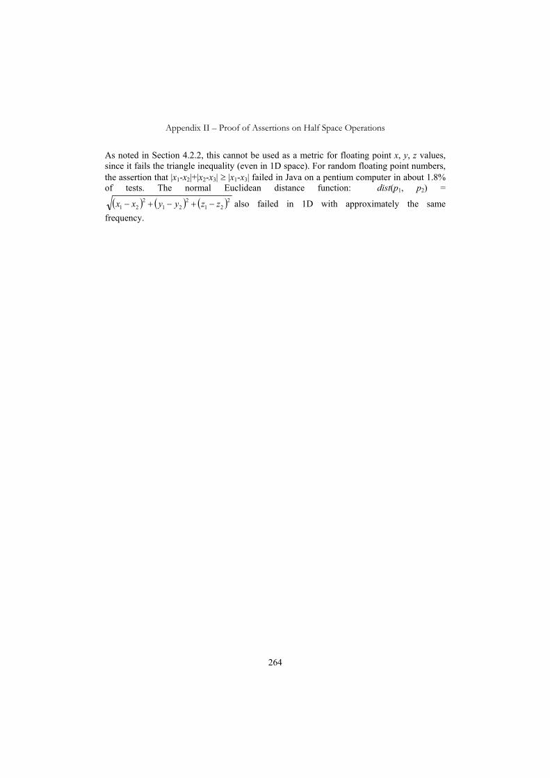
Appendix II – Proof of Assertions on Half Space Operations
264
As noted in Section 4.2.2, this cannot be used as a metric for floating point x, y, z values, since it fails the triangle inequality (even in 1D space). For random floating point numbers, the assertion that |x1-x2|+|x2-x3| ≥ |x1-x3| failed in Java on a pentium computer in about 1.8% of tests. The normal Euclidean distance function: dist(p1, p2) =
( ) ( ) ( )2212
212
21 zzyyxx −+−+− also failed in 1D with approximately the same frequency.

Appendix III Proof of Assertions for the Integer Interpretation
The proofs in this appendix are restricted to the integer interpretation of the regular polytope – where all points are represented as a triple of integer values p = (X,Y,Z) with X,Y,Z integers -M ≤ X,Y,Z < M. Note that only weak connectivity is addressed, and that the equivalent assertions for the strong (Cb) form of connectivity are not necessarily true in all cases.
III.1. For O≠OΦ, O≠O∞, Ca ),( OO (Sections 5.2.1 and 5.4)
This proof is based on the assumption that ε > 1, so that any two adjacent points are considered contiguous. Any smaller value of ε does not permit any contiguity of non-overlapping sets.
Let p = (X,Y,Z) be any point in O, X,Y,Z integers -M ≤ X,Y,Z < M. Either (X+1, Y, Z) ∈ O or ∈ O . If it is within O, try X+2 etc.
Let I” be max I>0, X+I < M: {(X,Y,Z) … (X+I,Y,Z)} ⊆ O. If X+I” < M-1, then point (X+I”,Y,Z) ∈ O and (X+I”+1,Y,Z) ∈ O , therefore Ca ),( OO . If X+I” = M-1, then try X-1, X-2 etc. Let I’ be max I>0, X-I ≥ -M: {(X-I,Y,Z) … (X,Y,Z)} ∈ O. If X-I” > -M, then point (X-I”,Y,Z) ∈ O and (X-I”-1,Y,Z) ∈ O , therefore Ca ),( OO .
Therefore Ca ),( OO unless p = (X,Y,Z) ∈ O ⇒ p’ = (X’,Y,Z) ∀ X’, -M ≤ X’ < M
The same reasoning can be applied to Y, showing that unless Ca ),( OO :
p = (X,Y,Z) ∈ O ⇒ p’ = (X’,Y’,Z) ∈ O, ∀ X’, Y’: -M ≤ X’, Y’ < M, and that p = (X,Y,Z) ∈ O ⇒ p’ = (X’,Y’,Z’) ∈ O, ∀ X’, Y’, Z’: -M ≤ X’, Y’, Z’ < M.
That is; Ca ),( OO or O = OΦ or O = O∞.
III.2. ∀ X,Y,Z∈O: Ca(X,Y∪Z) ⇔ [Ca(X,Y) ∨ Ca(X,Z)] (Section 5.2.1)
Ca(X,Y∪Z) means ∃ p ∈ Y∪Z and ∃ p’ ∈ X: dist(p, p’) < ε.
p ∈ Y∪Z ⇒ p ∈ Y or p ∈ Z Therefore Ca(X,Y) or Ca(X,Z)
Assuming Ca(X,Y) then ∃ p ∈ Y and ∃ p’ ∈ X: dist(p, p’) < ε.
p ∈ Y ⇒ p ∈ Y ∪ Z ⇒ Ca(X, Y∪Z).

Appendix III - Proofs of Assertions for the Integer Representation
266
Similarly Ca(X,Z) ⇒ Ca(X, Y∪Z).
Therefore [Ca(X,Y) ∨ Ca(X,Z)] ⇒ Ca(X, Y∪Z).
III.3. The Space of Regular Polytopes is a Discrete Boolean Connection Algebra under Ca (Section 6.4)
It has been shown in Appendix II that the set of regular polytopes forms a Boolean algebra. It is only necessary to show that it also satisfies the additional axioms for regular polytopes X, Y, Z:
(B1) C(X, Y) ⇒ C(Y, X) (B2) C(X, X) for X ≠ OΦ (B3) ∀ ),(:),( XXCOOXX ∞Φ≠ (B4) ∀ X ≠ OΦ, Y ≠ OΦ, Z ≠ OΦ: C(X,Y∪Z) ⇔ [C(X,Y) or C(X,Z)].
The axiom (B5) - ∀ X ≠ O∞, ∃ Y ≠ OΦ: ¬C(X,Y) is only satisfied by continuous (infinite) spaces.
B1: follows from the definition of Ca. B2 follows from the result that OV ⇒ Ca - noting that for X ≠ OΦ, OV(X,X). B3 was proved above in Appendix III.1. B4 was proved above in Appendix III.2.
III.4. The Space of Regular Polytopes is a Weak Proximity Space under Ca (Section 6.4.1)
The axioms are:
(PS1) A δ B ⇒ B δ A (PS2) (A ∪ B) δ C ⇔ A δ C ∨ B δ C (PS3) A δ B ⇒ A ≠ ∅ ∧ B ≠ ∅ (PS5) A ∩ B ≠ ∅ ⇒ A δ B.
For a weak proximity space, axiom PS41 is not required.
PS1: follows from the definition of Ca.
PS2: is a re-statement of axiom B4 of the Boolean Connection Algebra, and was proved in Appendix III.2.
PS3: follows from the definition of Ca, since ∀ O: ¬Ca(OΦ, O) and ¬Cb(OΦ, O).
PS5: is a restatement of OV ⇒ Ca.
1Axiom PS4 states that: A δ B ⇒ ∃ E: A δ E ∧ (X-E) δ B

Appendix IV Proofs of Assertions for the Dr-Rational Interpretation
The proofs in this appendix are restricted to the dr_rational representation. The terms grid2 number and grid2 point will be used as shortened terms for the dr-rational numbers and points based on numbers r = I/J with
–N'' ≤ I ≤ N'' 0 < J ≤ N' For 3D applications N' = 6M3, N'' = 6M4. (f4.30) For 2D applications N' = 2M2, N'' = 2M3. (f4.31)
The set of all grid2 points will be notated as G2, where p=(x, y, z) ∈ G2 if an only if x, y, z are grid2 numbers, and –M ≤ x, y, z < M.
IV.1. The Vertex Test for Redundant Half Spaces (Section 4.4.3)
This following test allows a considerable simplification in the algorithms that can be written to manipulate regular polytopes, by reducing the number of special cases that need to be accommodated. The following lemma shows that a simplified containment test can be applied, rather than that specified in the half-space definition. Put simply – the details of the relation operator can be ignored, and a simple test ≥ can be used. For example, in Figure IV-1, the half plane H is redundant to the definition of C, even though it passes through a vertex.
C
H
Figure IV-1 Vertex test for redundancy.
The importance of this lemma is that in the implementation of an algorithm to simplify the complex polygons, it is sufficient to test that all vertex points of a bounded convex polygon are within the pseudo-closure of a half plane to declare that half plane redundant. Various

Appendix IV - Proofs of Assertions for the Dr-Rational Representation
268
algorithms (such as the conversion of a general polygon to a regular polytope) result in cases similar to Figure IV-1, which would otherwise require tedious special case testing.
This result is very useful in implementing a database structure based on the regular polytope concept, since it allows the code which removes redundant half spaces or planes to be made much simpler. The testing of many special cases can be avoided.
Proposition 1:
If H is a halver1 such that Cpc ⊆ Hpc, then C ⊆ H. That is to say that if every point in Cpc is also within Hpc, then every point in C must also be within H, (and therefore H is redundant to the definition of C).
IV.1.1. Outline of proof that Cpc ⊆ Hpc ⇒ C ⊆ H
The first step is to show that the intersection of an n dimensional halver/convex polytope with a hyperplane is itself a valid n-1 dimensional halver/convex polytope, provided that the hyperplane is of the form xn = c where xn is the last2 coordinate.
The remainder of the proof is by induction. Assuming the proposition is true for n-1 dimensions, it is shown to hold for n dimensions. Finally, the proposition is shown to hold for 1 dimension.
Figure IV-2 The n-1 dimensional object defined by the intersection of a convex
polytope with a hyperplane xn=c, is itself a convex polytope containing every point. from the original polytope with xn=c.
1 In this proof, the term “halver” is used to mean half plane, half space etc, depending on the dimension. 2 “Last” in this sense is the last coordinate to be mentioned in the definition of ρ at line (IV.1) (next page).

Appendix IV - Proofs of Assertions for the Dr-Rational Representation
269
A changed notation is required for this proof to allow for variable dimensionality. The vector notation for points is used, e.g. x = (x1, x2 , .. xn), with vectors in bold.
Let H(A1,A2 … An, B) be a halver in n dimensions defined as:
x = (x1, x2 , .. xn) ∈ H(A1,A2 … An, B) if A1x1 + A2x2 +… + Anxn + B ρ 0 – where (IV.1)
ρ is ≥ if A1>0, ρ is > if A1<0, ρ is ≥ if A1=0, A2>0, ρ is > if A1=0,A2<0, etc. ρ is ≥ if A1..An-1 = 0, An>0 ρ is > if A1..An-1 = 0, An≤0
An n dimensional halver is valid if:
A1 … An and B are integers, -M ≤ A1 … An ≤ M, (IV.2) -nM2 ≤ B ≤ nM2, (IV.3) and if A1 = A2 = … = An = 0, then B≠0. (IV.4)
Hpc is defined as x ∈Hpc if
A1x1 + A2x2 +… + Anxn + B ≥ 0 (IV.5)
Let C = {H1…Hm} be a convex polytope defined by m halvers defined as follows:
H1 = H(A11, A12, … A1n, B1) H2 = H(A21, A22, … A2n, B2) …. Hm = H(Am1, Am2, … Amn, Bm)
so that Hj is defined as 0ρ1
jji..ni
ji BxA +∑=
C is defined as {x: x∈Hj, j=1..m}. Cpc is defined as {x: x∈Hj
pc, j=1..m}.
IV.1.2. Lemma - induction on halvers
The intersection of n-dimensional halver (n>1), H(A1,A2 … An, B) with the hyperplane xn = x’n (where x’n is a constant –M ≤ x’n < M) is itself a n-1 dimensional halver H-. Further, any point x∈H- is an element of H, and any point x∈H with xn = x’n is an element of H-.
Let B” = Anx’n + B, (IV.6)
The halver H(A1, A2 … An-1, B”) would fulfill the requirements of a valid n-1 dimensional halver if :
A1 … An-1 and B” are integers, -M ≤ A1 … An-1 ≤ M,

Appendix IV - Proofs of Assertions for the Dr-Rational Representation
270
-(n-1)M2 ≤ B” ≤ (n-1)M2 and if A1 = A2 = … = An-1 = 0, then B”≠0.
While the first two requirements are obviously satisfied, the latter two are not necessarily true, but with the following modifications, a valid halver can be assured.
If B” < -(n-1)M2, then let B’ = -(n-1)M2. 3 (IV.7) If B” > (n-1)M2, then let B’ = (n-1)M2. 4 (IV.8) If A1 = A2 = … = An-1 = 0, and B”=0, then
let B’ = 1 if An >0, let B’ = -1 if An ≤ 0. (IV.9)
Otherwise, B’ = B”.
It is clear that this is now a valid n-1 dimension halver.
let x- = (x1, x2, …xn-1) be a n-1 dimensional point x- ∈ H- and let x+ = (x1, x2, …xn-1, x’n) be that point extended to n dimensions on the plane xn = x’n
Case 1 A1..An-1 are not all zero, B’ = B”,
x- ∈H- ⇒ B'xA i..ni
i +∑−= 11
ρ 0 (note – that ρ has the same definition as in the n
dimensional halver based on A1 to An-1). ⇒ Bx'AxA nni
..nii ++∑
−= 11 ρ 0 (substituting IV.6)
⇒ x+∈ H.
Case 2 A1..An-1 are not all zero, B” < B’
B’ = -(n-1)M2 (by IV.7) and B” < -(n-1)M2. (IV.10) Since each Ai ≥ -M, and each –M ≤ xi < M, 2
111)M(nxA i
..nii −≤∑
−=
.
Consider BxA i..ni
i +∑=1
= BxAxA nni..ni
i ++∑−=
'11
≤ (n-1)M2 + B” (by IV.6) < 0 (by IV.10) Thus, there is no point x- in H-.
3 In fact, this is equal to the universal halver, since the sum of the Aixi terms can never be < -(n-1)M2, and to reach this requires a point p = (x1, x2 .. xn-1) (–M ≤ xi < M), this requires all xi = -M and all Ai = M. Point p is such that A1x1+ A2X2 + …An-1-Xn-1 +B’ = 0 and since A1 is positive, x ∈ H. For all other x and for all other Ai, , A1x1+ A2X2 + …An-1-Xn-1 +B’ > 0, so all points are within H. 4 Similarly, this is equal to the empty halver.

Appendix IV - Proofs of Assertions for the Dr-Rational Representation
271
Case 3 A1..An-1 are not all zero, B” > B’
B’ = (n-1)M2 , and (by IV.8) B” > (n-1)M2. (IV.11) Consider x+ as defined above (such that x- ∈H-). x- ∈ H- ⇒ 0ρ
11B'xA i
..nii +∑
−=
⇒ 011
≥+∑−=
B'xA i..ni
i (IV.12)
Consider BxA i..ni
i +∑=1
= BxAxA nni..ni
i ++∑−=
'11
= "11
BxA i..ni
i +∑−=
(by IV.6)
> B'xA i..ni
i +∑−= 11
(by IV.8)
> 0. (by IV.12) Therefore x+ ∈H.
Case 4 If A1 = A2 = … = An-1 = 0, and B’>0
By definition of B’, either A1 = A2 = … = An-1 = 0, and B”>0 i.e. B” = Anx’n + B > 0 (by IV.6) i.e. BxA i
..nii +∑
=1 > 0
or A1 = A2 = … = An-1 = 0, and B”=0 i.e. Anx’n + B = 0 and An > 0. (by IV.9) i.e. BxA i
..nii +∑
=1 = 0, and A1 = A2 = … = An-1 = 0, An > 0
In either case, x+ ∈ H.
Case 5 If A1 = A2 = … = An-1 = 0, and B’<0
H- is empty.
So in all cases, x- ∈ H- ⇒ x+ ∈ H.
Conversely
Let x- = (x1, x2, …xn-1) be a n-1 dimensional point x- ∉ H-
Again let x+ = (x1, x2, … xn-1, x’n) be that point extended to n dimensions.
Case 1 A1..An-1 are not all zero, B’ = Anx’n + B,
x- ∉ H-
⇒ 0ρ_
11B'xA i
..nii +∑
−=
(where _ρ is the inverse of ρ)
⇒ 0ρ_
11Bx'AxA nni
..nii ++∑
−=
(by IV.6)
⇒ x+ ∉ H.

Appendix IV - Proofs of Assertions for the Dr-Rational Representation
272
Case 2 A1..An-1 are not all zero, B” < B’
B’ = -(n-1)M2, and (by IV.7) B” < -(n-1)M2. Consider x+ as defined above (such that x- ∉ H-). As above, 2
111)M(nxA i
..nii −<∑
−=
,
therefore 011
B"xA i..ni
i <+∑−=
,
therefore x+ ∉ H.
Case 3 A1..An-1 are not all zero, B” > B’
B’ = (n-1)M2 and (by IV.8) B” > (n-1)M2. As above, 2
i1..1
i 1)M(nxA −−>∑−= ni
,
therefore 011
>+∑−=
B"xA i..ni
i .
Thus every point x- must be in H-.
Case 4 If A1 = A2 = … = An-1 = 0, and B’>0
No point x- can exist such that x- ∉ H-.
Case 5 If A1 = A2 = … = An-1 = 0, and B’<0
By definition of B’, Anx’n + B < 0 or Anx’n + B = 0 and An ≤ 0. In either case, x+ ∉ H.
So in all cases, x- ∉ H- ⇒ x+ ∉ H.
Alternatively, any point x ∈ H with xn = x’n is an element of H-.
Corollary – induction on convex polytopes
If C is a convex polytope C = {H1…Hm}, and the intersection Hj- of each Hj (j=1..m) with
the plane xn = x’n is formed as above, the set C- = {H1-…Hm
-} is a n-1 dimensional convex polytope. Further, for any point x ∈ C- ⇒ x ∈ C, and for any point with xn = x’n, x ∈ C ⇒ x ∈ C-.
This follows from the definitions.
Corollary – induction on halver pseudo-closure
The intersection of the pseudo-closure of a n-dimensional halver (n>1), Hpc with the hyperplane xn = x’n (where x’n is a constant –M ≤ x’n < M) is itself a n-1 dimensional halver pseudo-closure H-pc. Further, any point x- ∈ H-pc ⇒ x+ ∈ Hpc, and for any point with xn = x’n, x ∈ Hpc ⇒ x-∈ H-pc.
This follows using the logic of the above lemma.

Appendix IV - Proofs of Assertions for the Dr-Rational Representation
273
Corollary– induction on convex polytope pseudo-closure
If Cpc is a the pseudo-closure of a convex polytope Cpc = {H1pc…Hm
pc}, and the intersection Hj
-pc of each Hjpc (j=1..m) with the plane xn = x’n is formed as above, the set C-pc = {H1-
pc…Hm-pc} is the pseudo-closure of an n-1 dimensional convex polytope. Further, any point
x-∈C-pc ⇒ x+∈Cpc, and for any point x with xn = x’n, x∈Cpc ⇒ x-∈ C-pc.
This follows from the definitions.
IV.1.3. Proof of Vertex Test for Redundant Half Spaces
In n dimensions, let H be a halver such that every point in Cpc is within Hpc.
Assume that the proposition is true for dimension n-1. (The iterative assumption)
Let x’ = (x’1, x’2, .. x’n) be any point which is within C.
x’ ∈ C ⇒ x’ ∈ Cpc ⇒ x’ ∈ Hpc. (IV.13)
Consider the hyperplane defined by x’n (all points with xn = x’n), and the intersection of C and H with this hyperplane (named C- and H- respectively):
Let x- = (x-1, x-
2 , .. x-n-1) be any point in C-pc, then it follows that
x+ = (x-1, x-
2 , .. x-n-1, x’n) ∈Cpc
,
x+ ∈ Cpc ⇒ x+ ∈ Hpc
x+ ∈ Hpc, ⇒ x- ∈ H-pc
Thus any point in C-pc is also in H-pc. Therefore, by the iterative assumption, H- is redundant
to the definition of C-, i.e. x-∈C- ⇒ x-∈ H-.
But x’ ∈ C ⇒ (x’1, x’2, .. x’n-1) ∈ C- ⇒ (x’1, x’2, .. x’n-1) ∈ H-.
(x’1, x’2, .. x’n-1) ∈ H- ⇒ x’ ∈ H.
Thus x’ ∈ C ⇒ x’ ∈ H.
That is, if the proposition is true in n-1 dimensions, then it is true in n dimensions.
Consider the 1D case:
Let H(A, B) be a halver defined as:
x = (x) ∈ H(A, B) if Ax + B ρ 0 – where ρ is ≥ if A > 0, ρ is > if A ≤ 0.
Let C = {H1…Hm} be a convex polytope defined by m halvers defined as follows:
H1 = H(A1, B1) H2 = H(A2, B2) … Hm = H(Am, Bm) so that Hj is defined as Ajx+Bj ρj 0.
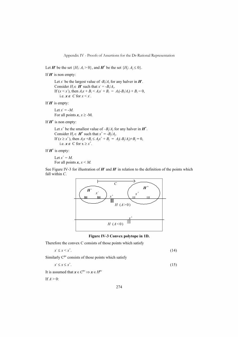
Appendix IV - Proofs of Assertions for the Dr-Rational Representation
274
Let H- be the set {Hi: Ai > 0}, and H+ be the set {Hj: Aj ≤ 0}.
If H- is non empty:
Let x- be the largest value of -Bi/Ai for any halver in H-. Consider Hi ∈ H- such that x- = -Bi/Ai. If (x < x-), then Aix + Bi < Aix- + Bi = Ai(-Bi/Ai) + Bi = 0, i.e. x ∉ C for x < x-.
If H- is empty:
Let x- = -M. For all points x, x ≥ -M.
If H+ is non empty:
Let x+ be the smallest value of –Bj/Aj for any halver in H+. Consider Hj ∈ H+ such that x+ = -Bj/Aj. If (x ≥ x+), then Ajx +Bj ≤ Ajx+ + Bj = Aj(-Bj/Aj)+Bj = 0, i.e. x ∉ C for x ≥ x+.
If H+ is empty:
Let x+ = M. For all points x, x < M.
See Figure IV-3 for illustration of H- and H- in relation to the definition of the points which fall within C.
x - x +
H (A > 0 )
H (A < 0 )
H + H -
C
x ’
x ’
Figure IV-3 Convex polytope in 1D.
Therefore the convex C consists of those points which satisfy
x- ≤ x < x+. (14)
Similarly Cpc consists of those points which satisfy
x- ≤ x ≤ x+. (15)
It is assumed that x ∈Cpc ⇒ x ∈Hpc
If A > 0:

Appendix IV - Proofs of Assertions for the Dr-Rational Representation
275
Let x’ = -B/A. H is defined as points x = (x) for which x ≥ x’, and H = Hpc. x ∈ C ⇒ x ∈ Cpc ⇒ x ∈ Hpc ⇒ x ≥ x’ ⇒ x ∈H, as required.
If A < 0
Let x’ = -B/A. H is defined as all points x = (x) for which x < x’, ': xxxH ≥= . But x’∈ Hpc . If x’ < x+, (x+) ∈ Cpc (by IV.15) (x+) ∈ Hpc ⇒ x+ ≤ x’ – contradiction – therefore x’ ≥ x+. x ∈ C ⇒ x < x+ (by IV.14) ⇒ x < x’ ⇒ x ∈ H. – as required.
If A = 0
If B < 0, then H is the empty halver, and there are no points in Hpc. Thus Cpc is also empty. Alternatively if B > 0, then this is the universal halver, and all points in C must be in H.
Thus the proposition is proved in 1 dimension.
Therefore it follows for all dimensions ≥ 1.
IV.2. Vertex Test for Incompatible Half Spaces (Section 4.4.3)
Taken in conjunction with proposition 1, this, in effect states that the complexity of the definition (in terms of the use of the ≥ or > relational tests) can be safely ignored while programming the simplification algorithms. The complexity of these two proofs is more than justified by the reduction in complexity they allow in the software.
Proposition 2
Hpx (the pseudo-exterior of H) is defined as:
x ∈Hpx if A1x1 + A2x2 +… + AnXn + B ≤ 0. (IV.16) Note that any point on the hyperplane of H is an element of Hpx and of Hpc.
If H is a halver5 such that Cpc ⊆ Hpx, then H is incompatible with C. That is to say that if every point in Cpc is also within Hpx, then every point in C is not within H.
IV.2.1. Outline of proof of proof that Cpc ⊆ Hpx ⇒ C ∩ H = CΦ
The proof, like that of IV.1, is by induction. Assuming the proposition is true for n-1 dimensions, it is shown to hold for n dimensions. Finally, the proposition is shown to hold for 1 dimension.
5 The term “halver” is used to mean half plane, half space etc, depending on the dimension.

Appendix IV - Proofs of Assertions for the Dr-Rational Representation
276
As before, let C = {H1…Hm} be a convex polytope defined by m halvers defined as follows:
H1 = H(A11, A12, … A1n, B1) H2 = H(A21, A22, … A2n, B2) …. Hm = H(Am1, Am2, … Amn, Bm). so that Hj is defined as ji
..niji BxA +∑
=1 ρj 0.
C is defined as {x: x∈Hj, j=1..m}. Cpc is defined as {x: x∈Hj
pc, j=1..m}.
IV.2.2. Corollary – induction on convex polytope pseudo-exterior
The intersection of the pseudo-exterior Hpx of a n-dimensional halver (n>1), with the hyperplane xn = x’n (where x’n is a constant –M ≤ x’n < M) is itself the pseudo-exterior H-px of the n-1 dimensional halver H- (defined in Appendix IV.1.2). Further, any point x- ∈ H-px ⇒ x- ∈ Hpx, and for any point with xn = x’n, x∈Hpx ⇒ x ∈ H-px.
This follows from the lemma of proposition 1.
IV.2.3. Proof of Vertex Test for Incompatible Half Spaces
Let H be a halver such that every point in Cpc is within Hpx.
Assume that the proposition is true for dimension n-1. (The iterative assumption)
Let x’ = (x’1, x’2 , .. x’n) be any point such that x’ ∈ C
x’ ∈ C ⇒ x’ ∈ Cpc ⇒ x’ ∈ Hpx.
Consider the hyperplane defined by x’n (all points with xn = x’n), and the intersection of C and H with this hyperplane (named C- and H- respectively).
Let x- = (x-1,x-
2 , .. x-n-1) be any point in C-pc, then it follows that
x+= (x-1, x-
2, .. x-n-1, xn) ∈Cpc
,
x+∈Cpc ⇒ x+∈Hpx
x+∈Hpx ⇒ x-∈H-px
Thus any point in C-pc is also in H-px. Therefore, by the iterative assumption, H- is
incompatible with C-. Therefore there can be no point in C- which is in H-.
But x’ ∈C ⇒ (x’1, x’2 , .. x’n-1) ∈C- ⇒ (x’1, x’2 , .. x’n-1) ∉H-.
(x’1, x’2 , .. x’n-1) ∉H- ⇒ x’ ∉ H.
Thus x’ ∈ C ⇒ x’ ∉ H.
i.e. if the proposition is true in n-1 dimensions, then it is true in n dimensions.
Consider the 1D case:
Defining H = H(A, B), and C = {H1…Hm} as in proposition 1,

Appendix IV - Proofs of Assertions for the Dr-Rational Representation
277
x - x+
H (A>0)
H (A<0)
C
x’
x’
H px
H px Figure IV-4 Relationship of x-, x+ and x’ to C and H.
As before, we can determine x- and x+ such that C is defined as
x = (x), such that x- ≤ x < x+. (IV.17)
Similarly Cpc becomes
x, such that x- <= x <= x+. (IV.18)
It is assumed that x ∈Cpc ⇒ x ∈Hpx
If A > 0:
let x’ = -B/A. H is defined as all points for which x ≥ x’. Hpx is defined as all points for which x ≤ x’. (IV.19) x+ ∈ Cpc ⇒ x+ ∈ Hpx ⇒ x+ ≤ x’. (by IV.19)
But x ∈ H ⇒ x ≥ x’ ⇒ x ≥ x+ ⇒ x ∉ C. (by IV.17) i.e. all points in H are excluded from C.
If A < 0
let x’ = -B/A. H is defined as all points for which x < x’ Hpx is defined as all points for which x ≥ x’. (IV.20) x- ∈ Cpc ⇒ x- ∈ Hpx ⇒ x- ≥ x’. (by IV.20)
But x ∈ H ⇒ x < x’ ⇒ x < x- ⇒ x ∉C. (by IV.17) i.e. all points in H are excluded from C.
If A = 0
If B < 0, then H is the empty halver, so no point in C may be in H. Alternatively if B > 0, then Hpx contains no points, so C must contain no points.
Thus the proposition is proved in 1 dimension.
Therefore it follows for all dimensions ≥ 1.
Appendix IV - Proofs of Assertions for the Dr-Rational Representation
278
IV.3. Lemma: every non-degenerate convex polytope contains at least one point with rational coordinates - p ∈ QQ3.
For this discussion, non-degenerate convex polytope is one which, after all redundant half spaces has been removed, consists of at least one half space, which is ≠ HΦ and ≠ H∞.
Let C be a non-degenerate convex polytope with no redundant half spaces. Let vk: k=1..m be the vertices of C. Since there is at least one non-redundant half space m > 0.
Otherwise, for every vertex vi = (xi, yi, zi), if xi > -M, then point (-M, yi, zi) ∈ C. Thus the half space at infinity H1
∞ = (1, 0, 0, M) is not redundant. But H1∞ has A > 0 - contradicton!
Let p = (x, y, z) = 1/m (v1+v2+… vm). (I.e. x = 1/m (x1 + x2 +… xm) etc.).
Since the field of rational numbers is closed under addition and division, x is a rational number.
The same applies to y and z, so that p ∈ QQ3.
For any Hi ∈ C:
Hi(p) = Aix + Biy + Ciz + Di = 1/m [(Aix1 + Biy1+Ciz1+Di) + (Aix2 + Biy2+Ciz2+Di) + … + (Aixm + Biym+Cizm+Di) = 1/m (Hi(v1) + Hi(v2) + … + Hi(vm))
but Hi(vk) ≥ 0, k=1..m therefore Hi(v) = 0 requires Hi(vk) = 0, k=1..3, which in turn means that all vk lie on Hi. Since all vk lie on Hi, they must be coplanar. Contradiction!
Therefore Hi(p) > 0 therefore p ∈ Hi for all Hi ∈ C.
Therefore p ∈ C.
Note – although this proof shows only that a point of arbitrary rational precision can be found in any non-degenerate convex polytope, it is highly probable that this can be tightened to state that a dr-rational point can be found, possibly requiring more precision than a grid2 dr-rational point.
IV.4. Uniqueness of Convex Polytopes (Section 4.4.5)
Consider two convex polytope definitions, C = {Hi: i=1..n} and C’ = {Hj’: j=1..m} such that p ∈ C ⇔ p ∈ C’ for any p ∈ QQ3.
For Hi ∈ C, there cannot be any vertex v’ of C’ such that v’ ∉ Hipc.
(Because if such a vertex existed, the three half spaces of C’ that define it and iH would together define a non-redundant convex polytope C”. Thus by IV.3, ∃ p” ∈ C”. This means p” ∈ C’ and p” ∉ H which contradicts the assumption.)
Thus every vertex v’ of C’ is within Cpc.
Likewise, every vertex v of C is within C’pc.

Appendix IV - Proofs of Assertions for the Dr-Rational Representation
279
Thus we have two convex polyhedra, each of which contains all the vertices of the other. This is no longer a specific problem of regular polytope or dr-rational number arithmetic, but a conventional geometric problem. It is clear by the convex nature of C and C’ that the vertices of each must be identical (otherwise there will be points within one, but not within the other), and that the faces that define each are coplanar.
Thus for every Hi ∈ C, there exists one H’j ∈ C’ such that Hi and H’j are coplanar, and vice versa. That is to say, there is a 1-1 correspondence between the half spaces that define C and C’, and for each pair Hi = (A, B, C, D) ∈ C and H’j = (A’, B’, C’, D’) ∈ C’, there exists a rational number r such that A = rA’, B = rB’, C = rC’, D = rD’.
IV.5. For O≠OΦ, O≠O∞, Cb ),( OO (Section 5.4)
First, given O = {Ci: i=1..n} where Ci = {Hij: j=1..m}, generate a convex coverage of the universal region, by dividing it by each Hij and its inverse. That is to say, start with the universal region, and split it into two between ijHO ∩∞ and ijHO ∩∞ . For each Hij added, the number of sub-regions will increase or remain the same (if this half space is coplanar with some other), but each sub-region will be convex. Let the universal region be divided into u subregions Sk: k=1..u, each being a convex polytope (see Figure IV-5).
Figure IV-5 Coverage (right) generated from a regular polytope (left).
The sub-regions will fall into two sets - }:{ OSS kk ⊆ and }:{ OSS ll ⊆ . Each sub-region
must be entirely within O or O , because all half spaces that define the original regular polytope are present in the coverage definition. It is also clear that any half space Hij (or its inverse) cannot further subdivide any sub-region. We ensure that all sub-regions are normalised to remove any redundant half spaces.
For any Sk = {Hki, i = 1..r} let C’ be the result of removing any Hkq from its definition (i.e. C’ = {Hki, i = 1..r: i ≠ q}.

Appendix IV - Proofs of Assertions for the Dr-Rational Representation
280
Sk Sl
Hkq
Figure IV-6 Subregion with a half space removed from its definition.
By the requirement that each sub-region has no redundant half spaces, there must be some p ∈ C’: p ∉ Sk. Because the set of sub-regions is a complete coverage, there must be some other sub-region Sl such that p∈ Sl (see Figure IV-6). Since the sub-regions are minimal, then Sl must contain all points p∈ C’ ∧ p ∉ Sk., and there can be no point p’ ∈ Sl: p’ ∉ C’. That is to say, C’ = Ck ∪ Cl.
In summary, the result of removing any half space from the definition of any sub-region is to create a convex polytope which is the union of two sub-regions.
Choose Ck and Hkq such that Sk ⊆ O and Sl ⊆ O . This must be possible unless O = OΦ or O = O∞. Thus we have
C’ ⊆ O ∪ O C’ ∩ Sk = Sk ≠ CΦ. C’ ∩ Sl = Sl ≠ CΦ.
Therefore Cb(O, O ).
IV.6. For O≠OΦ, O≠O∞, Ca ),( OO (Section 5.4)
This follows immediately from IV.3, since Cb ⇒ Ca.
IV.7. ∀ X,Y,Z∈O: Cb(X,Y∪Z) ⇔ [Cb(X,Y) or Cb(X,Z)] (Section 5.4)
This proof addresses a somewhat stronger statement of the proposition - that:
∀ X,Y,Z∈O: W = Y∪Z ∧ Cb(X,W) ⇔ [Cb(X,Y) or Cb(X,Z)],
W = Y∪Z ∧ Cb(X,W) makes the meaning explicit that set W which is pointwise equal to Y∪Z, but may have a different internal definition to Y and Z is connected to X.

Appendix IV - Proofs of Assertions for the Dr-Rational Representation
281
IV.7.1. Lemma ∀ X,Y,Z∈O: Cb(X,Y) ∧ Y=Z ⇒ Cb(X,Z)
That is to say if X is connected to Y and Y = Z then X is connected to Z. If OV(X,Y) the result is trivial, so the remainder of the proof assumes Cb(X,Y) ∧¬ OV(X,Y).
Cb(X, Y) ⇒ ∃ Cx ∈ X, Cy ∈ Y: Cb(Cx, Cy) - by definition of Cb ¬ OV(X,Y) ⇒ ¬ OV(Cx,Cy) Cb(Cx, Cy) ∧¬ OV(X,Y) ⇒ ∃Hx ∈ Cx, Hy ∈ Cy: yx HH ≅ by f5.1 Let C’x = {Hi: Hi∈Cx, Hi ≠ Hx} Let C’y = {Hj: Hj∈Cy, Hj ≠ Hy}.
That is to say, C’x is Cx with Hx omitted from its definition: Cx ⊂ C’x, and C’y is equivalent.
Let C = C’x ∩ C’y.
C is now a convex polytope which is contained within Cx ∪ Cy and has a non-empty intersection with both as illustrated in Figure IV-7 (see also Section 5.2).
Y
Cy
X Cx
Hx Hy
Figure IV-7 X and Y with overlapping convex polytope C shaded.
Let W = Z ∪ C. Convert W to maximal form, as described in Appendix IV.5. This divides the universal region into u subregions Sk: k=1..u, each being a convex polytope.
The sub-regions will fall into two sets: }:{' WSSW kk ⊆= and }:{' WSSW ll ⊆= . The set }:{ WSS kk ⊆ can be further divided into }:{' ZSSZ kk ⊆= and
}',':{' ZSWSSX kkk ∉∈= . That is to say, W’ is the set of subregions within W, Z’ is the set of subregions within Z and X’ is the set of subregions within C ∩ X.

Appendix IV - Proofs of Assertions for the Dr-Rational Representation
282
Z
C Sx Sz
Figure IV-8 W = Z ∪ C in maximal form with C shaded, and Sx and Sz shown.
Let Sx ∈ X’ such that Hx ∈ Sx. There must be at least one because C ∩ X is non-empty and is separated from Z by Hx (see Figure IV-8).
Let S = {H: H∈Sx, H≠Hx} i.e. S is Sx with Hx omitted from its definition. Let Sz = S – Sx i.e. Sz is the region of S not within Sx. Let pz be a point: pz ∈ Sz. Assume pz ∉ C.
⇒ ∃ H ∈ C’x or H ∈ C’x such that pz ∉ H. But, by the maximal nature of the decomposition, Sz ⊆ H or Sz ⊆ H , Therefore pz ∉ H ⇒ Sz ⊆ H .
Let px ∈ Sx. Sx ∈ X’ ⇒ Sx ⊆ C ⇒ px ⊆ C⇒ px ⊆ C’x ∩ C’y
⇒ px ⊆ H ⇒ Sx ⊆ H. Thus H separates Sx and Sz, and therefore H = Hx (by def of Sz). Contradiction! Therefore pz ∈ C, and so Sz⊆ C.
Therefore S = Sx ∪ Sz is a convex polytope, its intersection with Cx is Sx ≠ CΦ, and its intersection with some Cz ∈ Z is Sz.
Thus, by definition Cb(Cx, Cz), and so Cb(X, Z).
IV.7.2. Proof that ∀ X,Y,Z∈O: Cb(X,Y∪Z) ⇔ [Cb(X,Y) or Cb(X,Z)]
Let X = {Ci, i=1..n}, Y = {Cj, j=1..o}, Z = {Ck, k=1..q},
let W’ = Y∪Z = {Cj, j=1..o, Ck, k=1..q}.
If Cb(X,W’), by definition: ∃ Ci ∈ X, Cl ∈ W’, Cb(Ci, Cl).
But by definition, Cl ∈ Y or Cl ∈ Z. Therefore, Cb(X,Y) or Cb(X, Z).
If Cb(X, Y) by definition, ∃ Ci ∈ X, Cj ∈ Y, Cb(Ci, Cj).
But Cj ∈ Y ⇒ Cj ∈ W’. Therefore, Cb(X, W’).

Appendix IV - Proofs of Assertions for the Dr-Rational Representation
283
Similarly, Cb(X, Y) ⇒ Cb(X, W’).
Since W = W’, applying the lemma,
∀ X,Y,Z∈O: W = Y∪Z ∧ Cb(X,W) ⇔ [Cb(X,Y) or Cb(X,Z)].
IV.8. ∀ X,Y,Z∈O: Ca(X,Y∪Z) ⇔ [Ca(X,Y) or Ca(X,Z)] (Section 5.4)
Let X = {Ci, i=1..n}, Y = {Cj, j=1..o}, Z = {Ck, k=1..q}.
Let W = Y∪Z.
If Ca(X,W), by definition: ∃ Ci ∈ X, Cl ∈ W, Ca(Ci, Cl).
Therefore ∃ p ∈ Cipc, p ∈ Cl
pc. p ∈ Cl
pc ⇒ p ∈ Wpc ⇒ p ∈ Ypc or p ∈ Xpc
p ∈ Ypc ⇒ p ∈ Cjpc for some Cj ∈ Y ⇒ Ca(Ci, Cj) ⇒ Ca(X, Y)
p ∈ Zpc ⇒ p ∈ Ckpc for some Ck ∈ Z ⇒ Ca(Ci, Ck) ⇒ Ca(X, Z)
Therefore, Ca(X,Y) or Ca(X, Z).
The converse is proved using the same logic.
IV.9. The Space of Regular Polytopes is a Discrete Boolean Connection Algebra under Ca or Cb (Section 6.5)
It has been shown in Appendix II that the set of regular polytopes forms a Boolean algebra. It is only necessary to show that it also satisfies the additional axioms:
(B1) C(X, Y) ⇒ C(Y, X) (B2) C(X, X) for X ≠ OΦ (B3) ∀ ),(:),( XXCOOXX ∞Φ≠ (B4) ∀ X ≠ OΦ, Y ≠ OΦ, Z ≠ OΦ: C(X,Y∪Z) ⇔ [C(X,Y) or C(X,Z)].
The axiom (B5) - ∀ X ≠ O∞ , ∃ Y ≠ OΦ : ¬C(X,Y) is only satisfied by continuous (infinite) spaces.
B1: follows from the definition of Ca and Cb.
B2 follows from the result that OV ⇒ Cb ⇒ Ca.
B3 was proved above in Appendices IV.3 and IV.6 .
B4 was proved above in Appendices IV.7 and IV.8.
IV.10. The Space of Regular Polytopes is a Weak Proximity Space under Ca or Cb (Section 6.4)
The axioms are:
(PS1) A δ B implies B δ A (PS2) (A ∪ B) δ C iff A δ C or B δ C

Appendix IV - Proofs of Assertions for the Dr-Rational Representation
284
(PS3) A δ B implies A ≠ ∅ and B ≠ ∅ (PS5) A ∩ B ≠ ∅ implies A δ B.
For a weak proximity space, axiom PS4 6 is not required.
PS1: follows from the definition of Ca and Cb.
PS2: is a re-statement of axiom B4 of the Boolean Connection Algebra, and was proved in Appendices IV.7 and IV.8.
PS3: follows from the definition of Ca and Cb, since ∀ O: ¬Ca(OΦ, O), ¬Cb(OΦ, O).
PS5: is a restatement of OV ⇒ Cb ⇒ Ca.
IV.11. Storage Required for Rational Number Computations (Section 3.4.6)
For the purposes of discussion, assume that a plane is to be specified in the form Ax+By+Cz+D=0 to pass through three points with integer coefficients, each requiring 32 bits to represent them. As described in Section 3.4.6, the formula for the parameters are:
A = y1z2 - y1z3 + y2z3 – y2z1 + y3z1 – y3z2. (f3.4) D = x1(y2z3 - y3z2) + x2(y3z1 – y1z3) + x3(y1z2 – y2z1). (f3.5)
With B, and C similar to A.
Thus A, B and C will require more than 64 bits, and D requires more than 96 bits.
If we then take three of these planes, defined by A1x+B1y+C1z+D1=0, A2x+B2y+C2z+D2=0, A3x+B3y+C3z+D3=0, and form their point of intersection in homogeneous coordinates p=(Px,Py,Pz,Q), where:
321
321
321
CCCBBBAAA
Q = , (f3.6)
3
3
3
2
2
2
1
1
1
CBD
CBD
CBD
Px
−−−= ,
3
3
3
2
2
2
1
1
1
CD
A
CD
A
CD
APy −−−= ,
3
3
3
2
2
2
1
1
1
DBA
DBA
DBA
Pz
−−−= . (f3.7)
Thus Px, Py and Pz require more than 224 bits (32×7) and Q requires more than 192 bits (32×6).
In attempting to take the next step, the plane through points (Px1,Py1,Pz1,Q1), (Px2,Py2,Pz2,Q2) and (Px3, Py3, Pz3, Q3), we replace the formulae f3.4 and f3.5 with their homogeneous coordinate equivalent to give:
6Axiom PS4 states that: A δ B implies ∃ E such that A δ E and (X-E) δ B

Appendix IV - Proofs of Assertions for the Dr-Rational Representation
285
0
3333
2222
1111 =
QPPPQPPPQPPPQZYX
zyx
zyx
zyx (f3.8)
or:
A = (Py1Pz2Q3 - Py1Pz3Q2 + Py2Pz3Q1 – Py2Pz1Q3 + Py3Pz1Q2 – Py3Pz2Q1) etc. D = Px1(Py2Pz3 - Py3Pz2) + Px2(Py3Pz1 – Py1Pz3) + Px3(Py1Pz2 – Py2Pz1)
This means that now A, B, C require more than 640 bits (32×20), and D requires more than 672 bits (32×21).
Thus the cycle of forming planes through points, and intersecting these planes causes a tenfold increase in the storage requirements of the coefficients (from 64 to 640 bits, 96 to 672 bits).


Appendix V Selected Java Documentation
This appendix contains an edited selection of JavaDoc for the three main classes of the demonstration software. Note that none of the classes documented here are directly instantiated, and therefore do not have public constructors. These classes are all parents of 2D and 3D subclasses, and it is these subclasses that are instantiated, with constructors defined.
V.1. Class Polytope
*
Polytope
nrUnitsA: int; unitNrA[*]: int; nrUnitsB: int; unitNrB[*]: int; MBR: box;
ConvexPoly
static newPolytope(String) newPolytope(int) clone(int) addConvexPoly(ConvexPoly) isConnectedA() isConnectedB() size() getConvexPoly(int) draw(GWin) union(Polytope) unionWith(Polytope) intersection() print() toString() inverse() universe() isWithin(Polytope) equals(Polytope) connectsToA(Polytope) connectsToB(Polytope) properPartOf(Polytope) isNull() intersects(Polytope) properOverlap(Polytope) tangentialProperPartOfA(Polytope) tangentialProperPartOfB(Polytope) nonTangentialProperPartOfA(Polytope) nonTangentialProperPartOfB(Polytope) externallyConnectedToA(Polytope) externallyConnectedToB(Polytope) extend() flatten() getMBR() asPolygon() dimension()
Polytope2
Polytope3
* Halver
Figure V-1 Polytope class and subclasses

Appendix V Selected Java Documentation
288
Direct Known Subclasses:
Polytope2, Polytope3
public class Polytope
extends java.lang.Object
Title: Regular Polytope.
Description: A region defined as the union of a number of convex polytopes (see Figure V-1 and Section 8.2).
Method Detail
V.1.1. newPolytope
public static Polytope newPolytope(java.lang.String inp)
Decode the database form of the regular polytope. Parameters: inp - String form of the regular polytope as read from the database. Returns: The internal regular polytope decoded from the database form.
V.1.2. clone
public Polytope clone(int convexPolyCount)
Create a new regular polytope with extra capacity as specified. Parameters: convexPolyCount - the number of extra convex polytopes that are to be
accommodated.
V.1.3. newPolytope
public Polytope newPolytope(int convexPolyCount)
Create a new empty regular polytope with capacity as specified, of the same dimensionality as this polytope.
Parameters: convexPolyCount - the number of extra convex polytopes that are to be
accommodated.

Appendix V Selected Java Documentation
289
V.1.4. addConvexPoly
public void addConvexPoly(ConvexPoly poly)
Add the convex polytope to this regular polytope. (This is equivalent to this = this.union(poly)).
Parameters: poly - A convex polytope.
V.1.5. isConnectedA
public boolean isConnectedA()
Determine if the regular polytope is internally contiguous using Ca connectivity. Returns: True if the regular polytope is internally contiguous using the weak connectivity
criterion.
V.1.6. isConnectedB
public boolean isConnectedB()
Determine if the regular polytope is internally contiguous using Cb connectivity. Returns: True if the regular polytope is internally contiguous using the strong connectivity
criterion.
V.1.7. size
public int size()
Returns: The count of the number of convex polytopes defining this regular polytope.
V.1.8. getConvexPoly
public ConvexPoly getConvexPoly(int index)
Parameters: index - Valid values 0..this.size()-1. Returns: The convex polytope at position index.
Appendix V Selected Java Documentation
290
V.1.9. draw
public void draw(GWin gWin)
For debug only. Parameters: gWin - a graphics window.
V.1.10. union
public Polytope union(Polytope other)
Form the union of this regular polytope with the other. Parameters: other - The other regular polytope. Returns: The union of this regular polytope with the other.
V.1.11. unionWith
public void unionWith(Polytope other)
Set this regular polytope to the union of itself with the other. Parameters: other - The other regular polytope.
V.1.12. intersection
public Polytope intersection(Polytope other)
Form the intersection of this regular polytope with the other. Parameters: other - The other regular polytope. Returns: The intersection of this regular polytope with the other.
V.1.13. print
public void print()
Print the regular polytope definition for debug purposes.

Appendix V Selected Java Documentation
291
V.1.14. toString
public java.lang.String toString()
Overrides: toString in class java.lang.Object. Returns: The regular polytope definition as a string in db format.
V.1.15. inverse
public Polytope inverse()
Calculate a Regular Polytope which is the inverse of this one. Returns: a Regular Polytope which is the inverse of this one.
V.1.16. universe
public Polytope universe()
Generate a regular polytope which covers the universal region of the dimension of this regular polytope.
Returns: A universal regular polytope.
V.1.17. isWithin
public boolean isWithin(Polytope other)
Determines if this regular polytope is within the other. Parameters: other - The other regular polytope. Returns: True if every point in this regular polytope is within the other regular polytope.
V.1.18. equals
public boolean equals(Polytope other)
Determines if this regular polytope is equal to the other (Point set equality). Parameters: other - The other Regular Polytope. Returns: True if every point in this regular polytope is within the other and vice versa.

Appendix V Selected Java Documentation
292
V.1.19. connectsToA
public boolean connectsToA(Polytope other)
This is the basic Ca continuity test between this and another regular polytope. Note that this differs from "intersects" which requires a point in common between the regions. Continuity requires only contact between the regular polytopes.
Parameters: other - the other Polytope. Returns: True if there is any point of contact between the two polytopes. Note that the regular
polytopes do not themselves have to be contiguous.
V.1.20. connectsToB
public boolean connectsToB(Polytope other)
This is the basic Cb continuity test between this and another regular polytope. Note that this differs from "intersects" which requires a point in common between the regions. Continuity requires only contact between the regular polytopes. To qualify as Cb, there must be at lease a plane of contact in 3D, or a line in 2D.
Parameters: other - the other Polytope. Returns: True if there is strong contact between the two polytopes. Note that the regular
polytopes do not themselves have to be contiguous.
V.1.21. properPartOf
public boolean properPartOf(Polytope other)
Test for proper containment of this by another regular polytope. Parameters: other - the other Polytope. Returns: True if this polytope is within the other but not vice versa.
V.1.22. isNull
public boolean isNull()
Test for empty polytope. Returns: True if this polytope is null - i.e does not contain any points.

Appendix V Selected Java Documentation
293
V.1.23. intersects
public boolean intersects(Polytope other)
Test for intersection of this by another regular polytope (i.e. a non empty intersection).
Parameters: other - the other Polytope. Returns: True if these polytopes have a non-empty intersection.
V.1.24. properOverlap
public boolean properOverlap(Polytope other)
Test for proper overlap of this by another regular polytope (i.e. a non empty intersection, but neither polytope containing the other).
Parameters: other - the other Polytope. Returns: True if these polytopes have a non-empty intersection, but both sets have points
outside that intersection.
V.1.25. tangentialProperPartOfA
public boolean tangentialProperPartOfA(Polytope other)
Test for proper containment of this by another regular polytope, but with at least one point of contact between this and the exterior of the other polytope.
Parameters: other - the other polytope. Returns: True if this polytope is within the other but not vice versa, and there is at least one
point of contact between this polytope and the exterior of the other.
V.1.26. tangentialProperPartOfB
public boolean tangentialProperPartOfB(Polytope other)
Test for proper containment of this by another regular polytope, but with at least a plane of contact (in 3D, line of contact in 2D) between this and the exterior of the other polytope.
Parameters: other - the other polytope. Returns:

Appendix V Selected Java Documentation
294
True if this polytope is within the other but not vice versa, and there is strong contact between this polytope and the exterior of the other.
V.1.27. nonTangentialProperPartOfA
public boolean nonTangentialProperPartOfA(Polytope other)
Test for proper containment of this by another regular polytope, with no point of contact between this and the exterior of the other polytope.
Parameters: other - the other Polytope. Returns: True if this polytope is within the other but not vice versa, and there is no point of
contact between this polytope and the exterior of the other.
V.1.28. nonTangentialProperPartOfB
public boolean nonTangentialProperPartOfB(Polytope other)
Test for proper containment of this by another regular polytope, with no plane (or line in 2D) of contact between this and the exterior of the other polytope.
Parameters: other - the other Polytope. Returns: True if this polytope is within the other but not vice versa, and there is no Cb contact
between this polytope and the exterior of the other.
V.1.29. externallyConnectedToA
public boolean externallyConnectedToA(Polytope other)
Test for external (weak or strong) connection (Ca) to this by another regular polytope
Parameters: other - the other Polytope Returns: True if this polytope is at least Ca connected to the other, but does not overlap it.
V.1.30. externallyConnectedToB
public boolean externallyConnectedToB(Polytope other)
Test for strong external connection to this by another regular polytope Parameters:

Appendix V Selected Java Documentation
295
other - the other Polytope Returns: True if this polytope is strongly connected (Cb) to the other, but does not overlap it.
V.1.31. extend
public Polytope3 extend()
Extend the 2D polytope into 3D by projecting into a prism in the z direction. Returns: A convex poly which is one dimension larger (add a z dimension to the x and y).
V.1.32. flatten
public Polytope2 flatten()
Flatten the 3d polytope into 2D by intersecting with z=0. Returns: A convex poly which is one dimension smaller.
V.1.33. getMBR
public Box getMBR()
Returns: A minimum bounding rectangle surrounding the regular polytope.
V.1.34. asPolygon
public MultiPolygon asPolygon()
Returns: The regular polytope converted to conventional vertex representation. Note that if
the polytope was 3D, it is flattened first.
V.1.35. dimension
public int dimension()
Returns: The dimensionality of the polytope (2 or 3).

Appendix V Selected Java Documentation
296
V.2. Class ConvexPoly
* *
Polytope ConvexPoly
MBR: box
ConvexPoly2
ConvexPoly3
Halver
addHalver(Halver) size() vertexSize() getHalver(int) getVertex(int) inverse() intersect(ConvexPoly) toString() draw() empty() closureEmpty() connectionA() connectionB() print() extend(Box) compareWith() newPolytope(int) newConvexPoly(int) extend() flatten() clone() dimension() universe() universalPolytope()
Figure V-2 ConvexPolytope class and subclasses
Direct Known Subclasses:
ConvexPoly2, ConvexPoly3
public class ConvexPoly
extends java.lang.Object
Title: Convex Polytope.
Description: A convex region defined as the intersection of a number of half planes in 2D, or half spaces in 3D (See Figure V-2 and Section 8.2).

Appendix V Selected Java Documentation
297
Method Detail
V.2.1. addHalver
public void addHalver(Halver newHalver)
Add a half plane or half space to this convex polytope definiton. The final result will be that part of this convex polytope which is also within the half plane/space. I.e. the intersection of the convex polytope and the half plane/space.
Parameters: newHalver - the half plane/space to be included.
V.2.2. size
public int size()
Returns: The count of the number of half planes/spaces defining this convex polytope.
V.2.3. vertexSize
public int vertexSize()
Returns: The count of the number of vertices defining this convex polytope.
V.2.4. getHalver
public Halver getHalver(int index)
Parameters: index - Valid values 0..this.size()-1. Returns: Halver half plane/space at position index.
V.2.5. getVertex
public PointR getVertex(int index)
Parameters: index - Valid values 0..this.vertexSize()-1. Returns: The vertex at position index as a Point3R or a Point2R.

Appendix V Selected Java Documentation
298
V.2.6. inverse
public Polytope inverse()
Calculate a regular polytope (not necessarily convex) which is the inverse of this convex polytope.
Returns: a regular polytope which is the inverse of this convex polytope.
V.2.7. intersect
public ConvexPoly intersect(ConvexPoly that)
Form the intersection of this convex polytope with another. Parameters: that - the other convex polytope. Returns: the intersection of this convex polytope with another.
V.2.8. toString
public java.lang.String toString()
Overrides: toString in class java.lang.Object. Returns: the convex polytope definition as a string in db format.
V.2.9. draw
public void draw(GWin gWin)
For debug only. Parameters: gWin - the drawing window.
V.2.10. empty
public boolean empty()
Determine if this convex polytope has become empty. Empty means that there are no points inside the convex polytope. If the pseudo-closure has points during the determination of contact, an empty convex polytope may have faces and vertices.
Returns: True if this convex polytope has become empty.

Appendix V Selected Java Documentation
299
V.2.11. closureEmpty
public boolean closureEmpty()
Determine if the closure of this un-normalised convex polytope1 has become empty. Returns: True if this convex polytope has become empty.
V.2.12. connectionB
public boolean connectionB()
Determine if this un-normalised convex polytope is a connection for strong connectivity test. I.e. does this consist of a pair of degenerate faces only?
Returns: True if this convex polytope has become a degenerate connection for strong
connectivity test.
V.2.13. connectionA
public boolean connectionA()
Determine if this un-normalised convex polytope is a connecton for weak connectivity test. I.e. does the closure of this convex polytope contain at least one point.
Returns: True if this convex polytope has become become degenerate for weak connectivity
test.
V.2.14. print
public void print()
Print the convex polytope parameters for debug purposes.
V.2.15. extend
public void extend(Box mbr)
Extend the minimum bounding rectangle to include this convex polytope.
1 This and other methods are used in the compareWith method. In effect, the pair of convex polytopes are intersected with the result not being normalised. These three methods are then used to determine the overlap or degree of connectedness of the result.

Appendix V Selected Java Documentation
300
V.2.16. compareWith
public int compareWith(ConvexPoly that)
Compare this convex polytope with another. Parameters: that - The other ConvexPoly Returns: DISJOINT if the polytopes do not connect. CONTACTSa if the polytopes meet at a single point. CONTACTSb if the polytopes meet at a face (or overlaps). CONTAINED if this polytope is completely contained by the other (including
tangential containment). CONTAINS if this polytope completely contains the other (including tangential
containment). EQUAL if this polytope completely contains the other and vice versa.
V.2.17. newPolytope
public Polytope newPolytope(int size)
create a new empty regular polytope with capacity as specified, and the same dimensionality as this convex polytope.
Parameters: size - the number of convex Polytopes that are to be accommodated.
V.2.18. newConvexPoly
public ConvexPoly newConvexPoly(int size)
create a new convex polytope with capacity as specified, and the same dimensionality as this. Since it is created with no halvers, it is initially equal to the infinite convex polytope.
Parameters: size - the number of halvers that are to be accommodated.
V.2.19. extend
public ConvexPoly3 extend()
Extend the 2d convex poly into 3D by projecting into a prism. Returns: A convex poly which is one dimension larger (adding a z value to the x and y).

Appendix V Selected Java Documentation
301
V.2.20. flatten
public ConvexPoly2 flatten()
Flatten the 3d polytope into 2D by intersecting with z=0. Returns: A convex poly which is one dimension smaller.
V.2.21. clone
public ConvexPoly clone(int halverCount)
Parameters: halverCount - the number of extra capacity required. Returns: a new convex polytope equal to the old one, with extra capacity as required.
V.2.22. dimension
public int dimension()
Returns: the dimensionality of the polytope (2 or 3).
V.2.23. universe
public ConvexPoly universe(int size)
Returns: A universal convex polytope, of the same dimensionality as this.
V.2.24. universalPolytope
public Polytope universalPolytope()
Returns: A universal regular polytope, of the same dimensionality as this convex polytope.

Appendix V Selected Java Documentation
302
V.3. Class Halver
surroundedBy
1
A, B, D: int; p1, p2: Point2R
HalfSpace 3..*
A, B, C, D: int; p: Point3R[3..*]
HalfPlane
toString() inverse() equals(Halver) compareWith(Halver) print() includes(PointR) extend() flatten() isUniverse() clone() truncate(Halver) isNull()
Halver
Figure V-3 Halver class and subclasses
Direct Known Subclasses:
HalfPlane, HalfSpace
public class Halver
extends java.lang.Object
Description: A half plane or half space (depending on the dimension of the problem domain universe). (See Figure V-3 and Section 8.2).
Method Detail
V.3.1. toString
public java.lang.String toString()
Overrides: toString in class java.lang.Object. Returns: String the half plane or space parameters as a string in DB format.

Appendix V Selected Java Documentation
303
V.3.2. inverse
public Halver inverse()
The set theoretical inverse of this half plane/space. i.e. the resultant half plane or space contains all points which are not in this plane or space.
Returns: Halver a half space/plane defining all points not in this half space/plane.
V.3.3. equals
public boolean equals(Halver that)
The set theoretical equality of this half plane/space compared to the other. i.e. the two planes/spaces define exactly the same set of points.
Parameters: that - The other half plane/space. Returns: true if the two planes/spaces define exactly the same set of points.
V.3.4. compareWith
public int compareWith(Halver other)
Compare two half spaces/planes, returning the relationship between them. Parameters: other - The other half plane/space. Returns: The relationship as defined below:
EQUAL - if the half planes/spaces define the same set of points. CONTAINEDBY - if all points in this set are contained within the other set. CONTAINS - if this set contains all points in the other set. ANTIEQUAL - if there is no point in both sets, but every point is in one set or
the other. That is to say, the boundaries coincide but in opposite directions. DISJOINT - if there is no point simultaneously in both sets, but the sets are not
ANTIEQUAL. OVERLAP - if the two half planes/spaces overlap. This is overlap in the infinite
line/plane sense, i.e. the half space/plane boundaries are not parallel.
V.3.5. print
public void print()
Print the half space or plane parameters for debug purposes.

Appendix V Selected Java Documentation
304
V.3.6. includes
public int includes(PointR point)
Test if dr-rational point p lies within or on the edge of the half space or plane. Parameters: point - the point. Returns: 1 if the point is within, 0 if on the edge, -1 outside of the half space or half plane.
V.3.7. extend
public Halver extend()
Extend the half plane into a half space. Returns: a halver which is one dimension larger (adding a z value to the x and y).
V.3.8. flatten
public Halver flatten()
flatten the half space into a half plane. Returns: a halver which is one dimension smaller (setting the z value to zero).
V.3.9. isUniverse
public boolean isUniverse()
Returns: true if this half space or plane is equal to the universal region
V.3.10. clone
public java.lang.Object clone()
Overrides: clone in class java.lang.Object Returns: a copy of the halver.

Appendix V Selected Java Documentation
305
V.3.11. truncate
public void truncate(Halver thatH)
Truncate the face defined by this halver by removing that part of it which is not within the other half plane or half space. Calculation of the points of intersection use halvers rather than vertices to avoid rounding errors or increasing precision requirements.
Parameters: thatH - The halver to be used to truncate this face.
V.3.12. isNull
public boolean isNull()
Determine if this edge line or plane is part of the boundary of the convex polytope which contains it.
Returns: True if this face is null. False if this edge line or plane is part of the boundary of the convex polytope which
contains it. (That is to say, it has not been truncated out of existence).


Appendix VI Encoding of the Regular Polytope
In the Java coding that was developed as a proof of concept for the Regular Polytope approach (see Chapter 8), a simplified textural encoding was used for database storage. Simple text encoding was chosen for its ease of debugging and visibility of internal details. It would be expected that in a final implementation a binary encoding would be used, and perhaps additional objects would be stored (such as vertices) to provide faster processing. The following (Figure VI-1) is a diagram of the format used for encoding, Figure VI-2 is an example of the encoding of a 2D regular polytope and Figure VI-3 is an example of the encoding of a 3D regular polytope – the red parcel shown in Figure 8-7. This format (or an equivalent format expressed in XML) could potentially be used as a “well known text” format for the interchange of regular polytope data.
Encoding Meaning n Dimensionality (2 or 3) { Start of regular polytope ccc Number of convex polytopes in this regular
polytope [ hhh Number of halvers in this convex polytope (A aaa Value of A B bbb Value of B C For 3D half spaces only ccc Value of C, for 3D half spaces only D dddd Value of D ) ] uu The unit number } End of regular polytope
Figure VI-1 Encoding of the regular polytope.

Appendix VI Encoding of the Regular Polytope
308
2{3[4(A1000000000B-123291173D-69575189961077544) (A-1000000000B-26136927D58393007284472408) (A1000000000B31431823D-57996749042819608) (A1000000000B34920016D-57735712615021376)] 1[3(A1000000000B26175247D-58388182445082504) (A-1000000000B-41425581D57246948141295320) (A-1000000000B-19410078D58894463521045944)] 1[4(A22044640B-1000000000D-76164657185192560) (A-1000000000B-34920016D57735712615021376) (A-20797546B1000000000D76091499563579888) (A1000000000B19410078D-58894463521045944)]1}
Figure VI-2 Sample of a 2D regular polytope with 3 convex polytopes.
3{4[5(A209106769B-1000000000C0D-87474526385019632) (A-1000000000B96742947C0D67619782016733008) (A154141516B1000000000C0D65542411417979120) (A0B0C1000000000D-1620000000000) (A0B0C-1000000000D3369000000000)] 1[9(A1000000000B-96742947C0D-67619782016733008) (A124297655B-1000000000C0D-82353864426437184) (A42902139B-1000000000C0D-77439217084724288) (A-1000000000B-485290904C0D24057595685639176) (A154151941B1000000000C0D65541781852024560) (A0B0C-1000000000D3369000000000) (A321910248B312154508C1000000000D3926298596179034) (A167386483B162313705C1000000000D2041013821873728) (A55882393B-39480156C1000000000D-6330415395970066)] 1[9(A1000000000B485290904C0D-24057595685639176) (A-39306006B-1000000000C0D-72475406303075040) (A-122497336B-1000000000C0D-67452131525276536) (A-203536187B-1000000000C0D-62558733116505200) (A-1000000000B305424379C0D83245526342290960) (A154151941B1000000000C0D65541781852024560) (A0B0C-1000000000D3369000000000) (A-9290258B-60270964C1000000000D-3951380303692924) (A-2668660B-67894450C1000000000D-4921817835264868)] 1[6(A-1000000000B305424379C0D83245526342290960) (A154151941B1000000000C0D65541781852024560) (A0B0C-1000000000D1150000000000) (A-49838883B-1000000000C414957265D-71840804779952464) (A-111385607B-1000000000C414957265D-68124465446020072) (A-160311958B-1000000000C555632101D-65170280390171696)]1}
Figure VI-3 Sample of a 3D regular polytope with 4 convex polytopes as pictured in Figure 8-7.

Appendix VII Data Storage Requirement Estimates
In order to compare the storage requirements of the regular polytope approach with conventional vertex-defined approaches, a number of theoretic cases have been estimated. In each of the following, the size quoted is for a single object (polygon, polyhedron or regular polytope). An attempt has been made to ensure that the relative complexity of the object is directly comparable in all cases, but this cannot always be guaranteed. For example, the storage requirements of the regular polytope have a dependence on the number of points of concavity in the object, which is highly variable and dependant on the application domain. These estimates should be treated as indicative only. They are used principally in Chapter 7 as part of the comparison of various suggested database schemata.
VII.1. Summary of Schemas
The estimates to be found on later pages of this appendix have been tabulated for convenience in Tables VII-1 and VII-2 below. The details of the cases, and the assumptions can be found later in the appendix. Since the requirements for the various 2D and 3D regular polytope forms do not differ by much, only the 3D forms have been estimated for the approximated polytope forms.
Table VII-1 – Vertex Representations
2D Simple
2D Moderate
3D Large
3D Simple
3D Moderate
3D Large
No Topology 96 b 864 b 80 kb 404 b 5668 b 560 kb With
Topology 148 b 532 b 40 kb 230 b 1736 b 160 kb
Table VII-2 – Regular Polytope Representations
2D Simple
2D Moderate
3D Large
3D Simple
3D Moderate
3D Large
No Topology 144 b 1860 b 165 kb 212 b 2344 b 207 kb Shared Halver Topology 147 b 1927 b 172 kb 196 b 2148 b 187 kb Approximated – no
Topology 620 b 9268 b 920 kb
Approximated – with Shared Halver
626 b 9368 b 930 kb
Approximated – with Shared Surfaces
532 b 3054 b 300 kb

Appendix VII Data Storage Requirement Estimates
310
VII.2. Assumptions
To simplify the calculations, an object-oriented storage model is assumed, with each class on the database schema diagram being represented by a block of memory. No provision has been made for indexes or overheads required by the file handling system. In addition, the following assumptions have been made:
• Each object carries 40 bytes of attributes. • All pointers are 4 bytes long. • All integers require 4 bytes except the D parameter of the half space, which requires 8
bytes. • All coordinate values (x, y and z) are stored as 4 byte integers. • Each one-to-many relation requires a count of the number of member objects. • Where possible, member objects are physically placed within the owner object, and do
not require pointers. • Each one-to-many link requires a pointer to each member object. • Each one-to-many link requires a pointer to the head from each member. • Each many-to-many relation has two counters, plus the necessary pointers to objects at
each end of the relation.
In all cases, three representative objects are compared:
1. A very simple object – 4 sides in 2D, 6 faces in 3D.
2. A moderately complex object – 100 faces or sides. In the regular polytope representations, 100 half spaces are used.
3. A large object with 10000 sides, faces or half spaces.
Simple 4 sided polygon in 2d with 4 directly adjoining
polygons.
Simple 6 face polyhedron in 3D
with 8 vertices and 6 directly adjoining
polyhedra
Moderate 6 surface polyhedron in 3D with 100 vertices
and 6 directly adjoining polyhedra
Moderate 100 sided polygon in 2d with 4 directly adjoining
polygons.
A B C
d
Figure VII-1 Simple and moderate objects
Examples of the kind of objects are illustrated in Figure VII-1. In the case of data models that use topological encoding, it is assumed that a complete coverage of space is being stored, and no estimate is made for any “edge of the world” conditions (that is, each shared surface or linestring is assumed to have a region on both sides).

Appendix VII Data Storage Requirement Estimates
311
A further question in the 3D objects being modelled is the ratio between the number of surfaces patches and the number of vertices of a polyhedron. This number is constrained to a small range of values provided the vertices and edges are only used to define the shape of the surface (not, for example, being used to provide coloured patches or measurement points). As can be seen in Figure VII-2, the ratio of vertices to surface patches varies from 1:2 in the case of a hexagonal decomposition to 2:1 in the case of a triangulated surface. For simplicity a ratio of 1:1 is chosen in this appendix (which is credible for the cadastral domain).
Average 2 corners per face
Average one corner per face
Average one corner per 2 faces
Figure VII-2 Ratio of corners to surface patches.
In the data models in this chapter, a UML class diagram is used to describe the schema, but a simplified diagram is used for the storage estimates. In this form of diagram, as exemplified in Figure VII-3, the actual relations between object classes are omitted to avoid clutter. Instead, dashed lines indicate the relative cardinality of the sets of objects at each end of the line. Each object has its estimated size in the upper right corner.
Region 76 bytes
attributes 40b LBR 16b lineString count 4b ptr to lineString 16 direction
2
LineString 16/108/10008 b
ptrs to region 4b point count 4b ptr to points 8/100/10000b
4
On average, each region is associated with 4 lineStrings. Each lineString is shared between two regions. Hence on average there will be two line strings for each region.
Point 4 bytes
x, y, z 4b
1 2 25 2500
Where three numbers are shown, they refer to the simple, medium and large cases.
Figure VII-3 Examples of storage estimate diagram format.
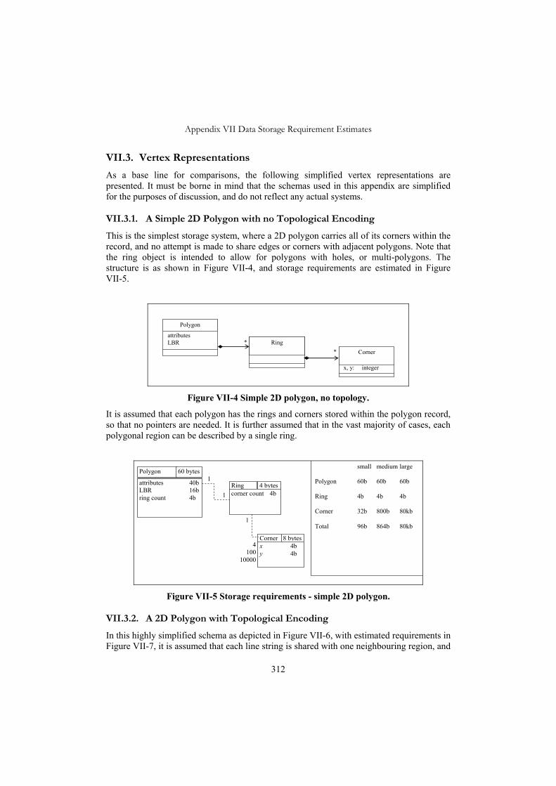
Appendix VII Data Storage Requirement Estimates
312
VII.3. Vertex Representations
As a base line for comparisons, the following simplified vertex representations are presented. It must be borne in mind that the schemas used in this appendix are simplified for the purposes of discussion, and do not reflect any actual systems.
VII.3.1. A Simple 2D Polygon with no Topological Encoding
This is the simplest storage system, where a 2D polygon carries all of its corners within the record, and no attempt is made to share edges or corners with adjacent polygons. Note that the ring object is intended to allow for polygons with holes, or multi-polygons. The structure is as shown in Figure VII-4, and storage requirements are estimated in Figure VII-5.
Polygon
Ring * attributes LBR
Corner *
x, y: integer
Figure VII-4 Simple 2D polygon, no topology.
It is assumed that each polygon has the rings and corners stored within the polygon record, so that no pointers are needed. It is further assumed that in the vast majority of cases, each polygonal region can be described by a single ring.
Polygon 60 bytes
attributes 40b LBR 16b ring count 4b
Corner 8 bytesx 4b y 4b
4 100
10000
1 Ring 4 bytescorner count 4b 1
1
small medium large Polygon 60b 60b 60b Ring 4b 4b 4b Corner 32b 800b 80kb Total 96b 864b 80kb
Figure VII-5 Storage requirements - simple 2D polygon.
VII.3.2. A 2D Polygon with Topological Encoding
In this highly simplified schema as depicted in Figure VII-6, with estimated requirements in Figure VII-7, it is assumed that each line string is shared with one neighbouring region, and

Appendix VII Data Storage Requirement Estimates
313
that there are four nodes in the boundary of each region (thus 4 linestrings) (see Figure VII-1A and B). It is also assumed that each node is common to four regions on average. The average number of linestrings for a region is therefore 4 – each shared with a neighbour. The average number points per region is the number of sides less the number of nodes.
direction
Region
Point *
attributes LBR
x, y: integer
Line String *
Node
*
x, y: integer
2
2
direction
Figure VII-6 a 2D polygonal region with topological encoding.
Region 80 bytes
attributes 40b LBR 16b lineString count 4b ptr to lineString 16b direction 4b
2
4
LineString 20 bytes ptr to region 8b ptr to node 8b point count 4b
4
2 Node 28 bytesx 4b y 4b lineString count 4b ptr to lineString 16b
Point 8 bytesx 4b y 4b
0 96
9994
1
1
2
small medium large Region 80b 80b 80b LineString 40b 40b 40b Node 28b 28b 28b Point 0b 384b 40kb Total 148b 532b 40kb
Figure VII-7 Storage requirements - 2D region with topology.
Note, in Figure VII-7, the 1-1 on the dotted line between Region and Node does not indicate a 1-1 link, but merely that on average the number of nodes in the database will be approximately the same as the number of regions.
VII.3.3. A Simple 3D Polyhedron with no Topological Encoding
This is the simplest possible storage system for a 3D polyhedron, where the faces are stored within the polyhedron, and the corners are stored within each face. Note that this allows for polyhedrons with holes, multi-polyhedrons and for faces with concavities. The structure is

Appendix VII Data Storage Requirement Estimates
314
as shown in Figure VII-8, with estimates in Figure VII-9. The simple polyhedron is a “brick” shape, with 6 faces and 8 corners, while in the complex cases the topology between regions is the same as in the simple case, but the surfaces of the regions are more detailed. (See Figure VII-1C and D).
Polyhedron
Ring *
attributes LBR
Corner *
x, y, z: integer
Face *
Figure VII-8 Simple 3D polyhedron, no topology.
Polyhedron 68 bytes
attributes 40b LBR 24b face count 4b
1
6 100
10000
Face 4 bytesring count 4b
1
1
1
4
1
small medium large Polygon 68b 68b 68b Face 24b 400b 40kb Ring 24b 400b 40kb Corner 288b 4800b 480kb Total 404b 5668b 560kb
Corner 12 bytesx 4b y 4b z 4b
24 400
40000
Ring 4 bytescorner count 4b
Figure VII-9 Storage requirements - simple 2D polygon.
VII.3.4. A 3D Polyhedron with Topological Encoding
Several different forms of topological encoding have been suggested in the literature (See Chapter 3). For comparison purposes, it is assumed that a simple structure is in use which shares the definition of surfaces between adjacent bodies. It is further assumed that there is very basic sharing of points within and between surfaces. It is assumed that each surface is shared with one neighbouring region, and that there are 6 surfaces in the boundary of each region.

Appendix VII Data Storage Requirement Estimates
315
direction
2
2
*
direction
Region
Node
attributes LBR
x, y, z: integer
Edge
2
Surface *
SurfacePatch *
Figure VII-10 a 3D polygonal region with topological encoding.
Region 98 bytes
attributes 40b LBR 24b surface count 4b ptr to surface 24b direction 6b
2
6
Node 12 bytesx 4b y 4b z 4b
2 Surface 12 bytes ptrs to region 8b surfacePatch count 4b
SurfacePatch 20 bytesnode count 4b ptr to node 16b
6 100
10000 1
4
6 100
10000
2
small medium large Region 98b 98b 98b Surface 36b 36b 36b SurfacePatch 60b 1000b 100kb Node 36b 600b 60kb Total 230b 1734b 160kb
Figure VII-11 Storage requirements - 3D region with topology.
VII.4. Regular Polytope Storage Estimates
It is not possible in general to estimate the number of convex polytopes per regular polytope for all application domains, and the numbers in practice are quite varied. For example, a regular polytope could consist of a single convex polytope defined by 20 half spaces. If the complement is taken of this, it will be a regular polytope of 20 convex

Appendix VII Data Storage Requirement Estimates
316
polytopes, each defined by one half space. It is felt that the proportions used in this appendix are reasonable, but the actual estimates are not particularly sensitive to this issue.
VII.4.1. A 2D Regular Polytope in Discrete Form
This is the basic form of storage of the regular polytope, as described in Section 7.2. Figure VII-12 shows the database objects only, omitting the face and vertex classes, which are only present during calculations. The storage estimates are as shown in Figure VII-13.
RegularPolytope
ConvexPolytope *
* HalfSpace
A, B, C, D: integer
Regular Polytope Representation
Figure VII-12 Regular polytope in simple form.
RegularPolytope 60 bytes
attributes 40b LBR 16b convexPoly count 4b
HalfPlane 16 A,B 8b D 8b
4 10 40
1
ConvexPoly 20 bytes halfPlane count 4b LBR 16b
1 10
250 1
small medium large RegularPolytope 60b 60b 60b ConvexPoly 20b 200b 5kb HalfPlane 64b 1600b 160kb Total 144b 1860b 165kb 1
4 100
10000
Figure VII-13 Storage requirements - 2D regular polytope.

Appendix VII Data Storage Requirement Estimates
317
VII.4.2. A 3D Regular Polytope in Discrete Form
This has the same schema diagram Figure VII-12, as the 2D equivalent. The 3D polytope storage requirements can be found in Figure VII-14.
Regular Polytope 64 bytes
attributes 40b LBR 24b convexPoly count 4b
HalfSpace 20 A,B,C 12b D 8b
6 10 40
1
ConvexPoly 28 bytes halverSpace count 4b LBR 24b
1 10
250 1
small medium large RegularPolytope 64b 64b 64b ConvexPoly 28b 280b 7kb HalfSpace 120b 2000b 200kb Total 212b 2344b 207kb
6 100
10000
1
Figure VII-14 Storage requirements - 3D regular polytope.
VII.4.3. A 2D Regular Polytope with Shared Half Planes
There is a further assumption required to estimate this structure’s requirements, and that is the degree to which halvers can be shared between convex polytopes. This depends on the application domain, and can be expected to be quite high for Cadastral data. The sharing rate could even be higher than the number of halvers per regular polytope (refer to Chapter 7 Figure 8, where the road frontages are shared by all parcels along the road). For the purposes of this estimate, it is conservatively assumed that halvers are shared between three convex polytopes on average. The schema is depicted in Figure VII-15, with the storage estimates in Figure VII-16.
A, B, C, D extents
* *
complement: Boolean
HalfSpace
Orientation RegularPolytope
ConvexPolytope 0:*
Figure VII-15 Shared half space topology.

Appendix VII Data Storage Requirement Estimates
318
Regular Polytope 68 bytes
attributes 40b LBR 16b convexPoly count 4b
HalfPlane 35 bytesA, B 8b D 8b convexPoly count 4b ptr to convexPoly 12b orientation 3b
4 10 40
1
ConvexPoly 40/70/220 bytes halfPlane count 4b ptr to halfPlane 16/40/160b orientation 4/10/40b LBR 16b
1 10
250
3
small medium large RegularPolytope 60b 60b 60b ConvexPoly 40b 700b 55kb HalfPlane 47b 1167b 17kb Total 147b 1927b 172kb 1
1.3 33.3 3333
Figure VII-16 Storage requirements, 2D shared half plane topology.
VII.4.4. A 3D Regular Polytope with Shared Half Spaces
Figure VII-17 shows the estimated requirements for the 3D equivalent – the regular polytope with shared half space topology.

Appendix VII Data Storage Requirement Estimates
319
Regular Polytope 68 bytes
attributes 40b LBR 24b convexPoly count 4b
HalfSpace 39 bytesA, B, C 14b D 8b convexPoly count 4b ptr to convexPoly 12b orientation 3b
6 10 40
1
ConvexPoly 50/78/228 bytes halfPlane count 4b ptr to halfPlane 16/40/160b orientation 6/10/40b LBR 24b
1 10
250
3
small medium large RegularPolytope 68b 68b 68b ConvexPoly 50b 780b 57kb HalfPlane 78b 1300b 130kb Total 196b 2148b 187kb 1
2 33.3 3333
Figure VII-17 Storage requirements - regular polytope in 3D with shared half spaces.
VII.4.5. 3D Approximated Regular Polytope
composed of
Body
Face
A, B, C, D: int
4..*
Boundary
1..*
Edge
3..*
Approximated Point
X, Y, Z: int13..*
bounded by
limited by other face
Figure VII-18 Approximated regular polytope.
This is the simplest form of the approximated polytope, and it is assumed that all faces, boundaries, edges and points are stored directly with the body. The other useful factors are that the “other face” relationship only needs to be navigated in the edge to face direction, and no back pointer is needed from approximated point to edge. Since the edges that define a boundary can be stored in order, only one approximated point per edge is needed.
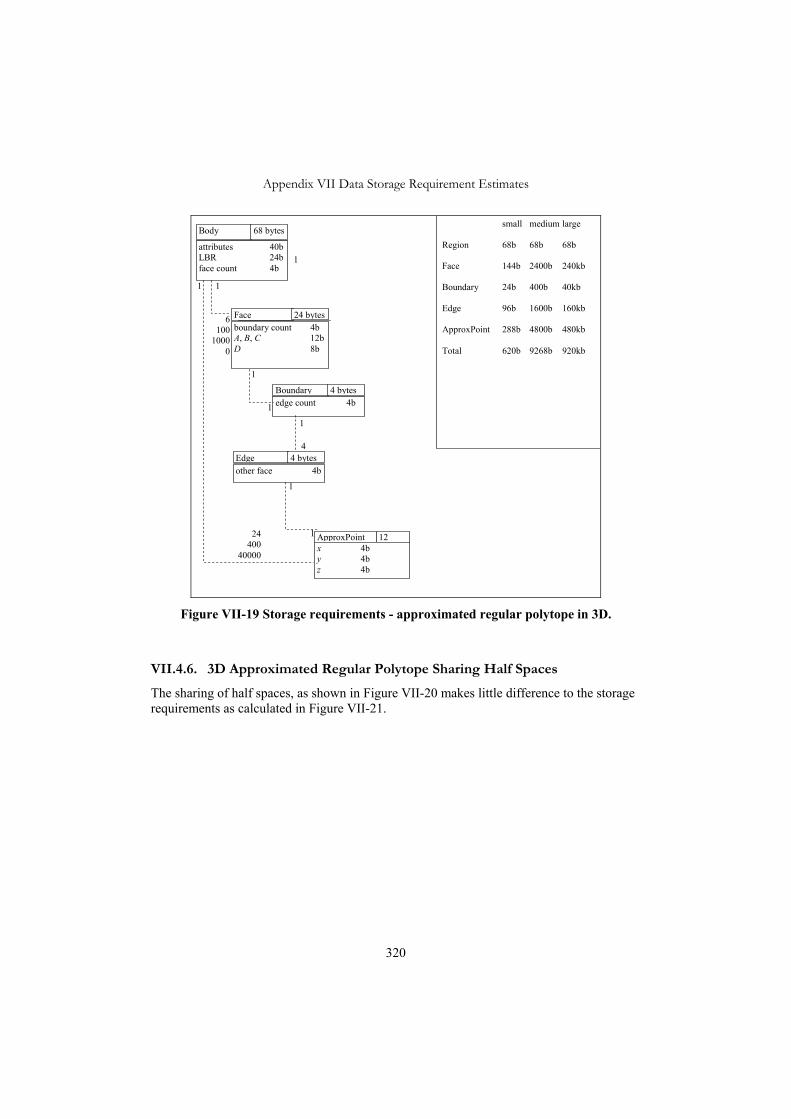
Appendix VII Data Storage Requirement Estimates
320
Body 68 bytes
attributes 40b LBR 24b face count 4b
1
6 100
10000
Edge 4 bytes other face 4b
1
1 ApproxPoint 12 x 4b y 4b z 4b
Face 24 bytes boundary count 4b A, B, C 12b D 8b
Boundary 4 bytesedge count 4b
1
4
1
24 400
40000
1
1
small medium large Region 68b 68b 68b Face 144b 2400b 240kb Boundary 24b 400b 40kb Edge 96b 1600b 160kb ApproxPoint 288b 4800b 480kb Total 620b 9268b 920kb
1
Figure VII-19 Storage requirements - approximated regular polytope in 3D.
VII.4.6. 3D Approximated Regular Polytope Sharing Half Spaces
The sharing of half spaces, as shown in Figure VII-20 makes little difference to the storage requirements as calculated in Figure VII-21.

Appendix VII Data Storage Requirement Estimates
321
*
1
complement: Boolean
1
Body
Facet
4..*
Boundary
1..*
Edge
3..*
1
Approximated Point
X, Y, Z: integer3..*
bounded by
limited by
composed of
other face
HalfSpace
A, B, C, D: intextents
Figure VII-20 Approximated regular polytope with shared half spaces.
Body 68 bytes
attributes 40b LBR 24b facet count 4b
1
6 100
10000
Edge 4 bytes other face 4b
1
1 ApproxPoint 12 x 4b y 4b z 4b
Facet 13 bytes boundary count 4b complement 1b halfSpace count 4b ptr to halfSpace 4b
Boundary 4 bytesedge count 4b
1
4
1
24 400
40000
1
1
HalfSpace 36 bytesA, B, C 12b D 8b facet count 4b ptr to facet 12b 3
3
6 100
10000
small medium large Region 68b 68b 68b Facet 78b 1300b 130kb HalfSpace 72b 1200b 120kb Boundary 24b 400b 40kb Edge 96b 1600b 160kb ApproxPoint 288b 4800b 480kb Total 626b 9368kb 930kb
1
Figure VII-21 3D Storage requirements approximated polytope with shared half
spaces.

Appendix VII Data Storage Requirement Estimates
322
VII.4.7. 3D Approximated Regular Polytope with Shared Surface Topology
This schema Figure VII-22 shares surfaces between adjoining bodies. There are savings over the earlier approximated polytope schemata, mainly in the sharing of points and edges, as can be seen in Figure VII-23. Note that for estimation purposes, the approximated edges are divided into two categories – those totally within one surface, and those that form the boundary between three or more surfaces – the “nodal edges”. This should provide a more accurate size estimate.
Surface Body
1..21..*
+ / -
Face
A, B, C, D: int
1..*
Boundary
1..* Approximate Edge Approximated Point
X, Y, Z: int22 *Left/R
ight
Figure VII-22 Approximated regular polytope with shared surface topology.

Appendix VII Data Storage Requirement Estimates
323
Surface 12 bytes
face count 4b ptrs to body 8b
6 100 10000
ApproxEdge 25 bytesother face 4bptr to point 8bboundary count 4bptr to boundary 8bdirection 1b
1
2 ApproxPoint 12 x 4b y 4b z 4b
Face 24 bytes A, B, C 12b D 8b boundary count 4b
Boundary 4 bytesedge count 4b
2
1
1
Body 98 bytesattributes 40b LBR 24b surface count 4b ptr to surface 24b +/- 6b
6
ApproxEdge 33 bytes other face 4b ptr to point 8 boundary count 4b ptr to boundary 16b direction 1b
2
2
12
2
1
2
0 88 9988
2
6 100 10000
where a “nodal edge”
small medium large Body 98b 98b 98b Surface 36b 36b 36b Face 72b 1200b 120kb Boundary 12b 200b 20kb Approx NodalEdge 198b 198b 198b ApproxEdge 0b 1100b 125kb AppproxPoint 72b 600b 60kb Total 488b 3432b 325kb
Figure VII-23 Storage requirements - approximated regular polytope with shared surfaces.


Summary
The storage and retrieval of spatial data in computer systems has matured greatly over recent years, from the earliest approaches (of simple digitised linework and text) to the representation of features and their attributes, with the semantics of their behaviour associated. This has led to massive cost savings where data, which might have been captured for a specific purpose, can be shared and reused for other purposes.
In this first generation of Geographic Information Systems (GIS), the data is stored locally, with each vendor using different nomenclature and definitions of spatial objects and having very different rules for what is accepted as “valid”. As a result a scientist using a desktop GIS may need to expend a considerable portion of his/her research effort and funds in translating, cleaning and preparing pre-existing data to convert to the form required for the study.
For some years now, there has been a trend towards spatial data being housed within a database management system, these being considered as a corporate resource, leading to the realisation that the geographic data itself is in fact an infrastructure, in the same way as is, for example, a telephone network. This moves the ownership of the data from the desktop, firstly to the corporation, and ultimately to being a shared resource between public and private organisations – a Geographic Information Infrastructure (GII).
An inhibiting factor in these trends is the lack of standardisation alluded to above. Where every data sharing operation involves manual intervention, it is difficult, if not impossible to create a GII. Thus a strong and consistent set of standards is needed, with the most basic requirement being for consistency in the geometric concepts used. While progress is being made by groups such as the International Standards Organisation Technical Committee 211 (ISO TC211) and the Open Geospatial Consortium (OGC), there is still much to be done.
The success of these standardisation efforts has been compromised by the requirement to be vendor neutral – i.e. to avoid specifying an internal representation to be used for storage. For example, the standards will remain silent on whether coordinate values should be stored in floating point or integer format.
As a result, definitions of spatial objects are expressed in mathematical terms assuming an infinite precision real number system, with the details of how this is to be translated into the computational representation being left to the implementer. Therefore there is no agreed normative meaning of the “equals” predicate when applied to geometric objects, and definitions of validity are in general left to the implementers.
If the standardisation effort is to allow spatial data to be interchanged without expensive manual intervention, a well defined logic is needed to underpin the standards and support the definition of validity of that data. This would also ensure that inferences drawn from the digital model remain consistent and do not lead to logical fallacies.

Summary
326
The language of spatial databases is couched in the language of mathematics, with operations being given names such as “union” and “intersection” and using vector-like representations. This naturally leads to the impression that the representations form a topological and/or vector space. Unfortunately this is not the case. Generally speaking, the rigorous mathematics used in the definition of spatial objects ends outside the database representation, which is only an approximation of the theoretical formalism used to define it.
This thesis documents a number of cases that illustrate the potential breakdown of logic to be found in current technology, for example, cases where the union or intersection operations lead to inconsistent results. Various alternative approaches that have been investigated in search of solutions are discussed, and their advantages and disadvantages indicated.
This current research has been motivated by an attempt to apply the mathematical approach to the actual representation of spatial features within the computer system. In this rigorous approach, the assumptions (or “axioms”) are clearly identified, and used to develop a chain of argument, leading to a proof of the required proposition. The advantage of this approach in the field of spatial data representation is that, if the computer hardware can be verified to obey the axioms, then the correct results of the algorithms are assured.
In order to facilitate such a chain of proof, a form of representation known as the regular polytope has been defined, based on a small set of axioms and definitions, and shown to possess a consistent and complete logic. That is to say, the computational representation itself expresses the algebraic formalism, rather than being an approximation to an idealised mathematical model.
Thus this representation is capable of providing a potential storage structure for a useful class of features, but this should not be seen as the sole object of the research. Rather the regular polytope should be seen as an exemplar for any approach to spatial data representation and storage.
The fact that this particular representation can be axiomatically defined and implemented demonstrates that such an approach is feasible, and opens the possibility that all computational representations can be similarly analysed. The regular polytope is a particularly tractable construct for this type of analysis, which is the reason for choosing it. By contrast the kind of structure embedded in many current systems is far more complex. In particular, floating point numbers add a significant level of complexity, and only the most basic topological behaviour has been proved where floating point operations are assumed.
Based on integer and domain restricted rational arithmetic, it is shown that the logic of topology, the Boolean connection algebra and the region connection calculus can be expressed directly by the database implementation. Thus a database built on this structure cannot suffer from the kinds of breakdown of logic discussed above. In addition, this raises the prospect of a definition of validity and robustness of representation that is not vendor specific.
A regular polytope representation of spatial objects is defined as the union of a finite set of (possibly overlapping) "convex regular polytopes", which are in turn defined as the

Summary
327
intersection of a finite set of half spaces. These half spaces are defined by finite precision number representations. The term “Regular Polytope” here does not carry its conventional meaning as the generalisation of a regular polyhedron (one having equal sides, faces and angles etc.). In the form used here, it combines the topological term “regular” with the conventional geometric meaning of “polyhedron”.
The actual definition is given in axiomatic form, structured so as to form a “boundary free” representation, valid in any number of dimensions. Although it is explored here principally in 3D, particular reference is made to the mixture of 2D and 3D found in many current application areas such as cadastral property boundaries. Particular attention is paid to the issue of connectivity, both within and between regular polytopes, and the resultant logic is developed in terms of well studied concepts such as the region connection calculus.
The particular representation chosen for the half space is such that adjoining regular polytopes will have no points in common, and no points will exist between them. Thus it is possible to define a complete partition of space where every point that can be represented computationally is defined to exist in one and only one region. In the traditional representations of 2D polygons and 3D polyhedrons, points play a very important role of carrying the metric information. This is in contrast to regular polytopes where points do not play a role in the definition at all. Instead the metric is specified via the half planes using 3 or 4 integers (in 2D and 3D respectively).
This theoretic basis is then applied to actual database schema design, and several alternative models proposed and analysed. As a check on the practicality of the algorithms, “proof of concept” classes have been developed in the Java programming language, and tested on a significant set of cadastral parcels (2D and 3D) from the Queensland cadastre.
Finally, further areas of research are identified, including extensions of the approach to wider problem domains.


Nederlandse Samenvatting
De opslag en bevraging van ruimtelijke gegevens in computersystemen heeft de laatste jaren flinke vooruitgang geboekt, vanaf het allereerste begin (digitaliseren van het lijnenwerk en de tekst) tot aan de huidige representatie van objecten en attributen, aangevuld met de semantiek. Dit heeft geleid tot een enorme kostenbesparing daar waar gegevens, die voor een bepaald doel worden ingewonnen en bijgehouden, nu ook gedeeld en hergebruikt kunnen worden voor andere toepassingen.
In de eerste generatie GIS had elke leverancier zijn eigen begrippenkader met bijbehorende definities van ruimtelijke objecten waarbij zeer verschillende regels werden toegepast om te bepalen wanneer een ruimtelijk object als geldig werd gezien. Momenteel kan een wetenschapper die een GIS gebruikt gedwongen zijn een aanzienlijk gedeelte van zijn/haar onderzoeksinspanning en -fondsen te besteden aan het vertalen, opschonen en voorbereiden van reeds bestaande gegevens om deze in de vorm te krijgen die voor het onderzoek nodig is.
Gedurende enige tijd is er een ontwikkeling richting het beheer van ruimtelijke gegevens in een database management systeem, dat als collectief bedrijfsmiddel wordt beschouwd. De volgende fase in deze ontwikkeling is het besef dat geografische gegevens zelf onderdeel van de infrastructuur zijn, vergelijkbaar met bijvoorbeeld een telefoonnetwerk. Hiermee verhuist het beheer van de gegevens van de lokale computer, via de bedrijfsorganisatie, uiteindelijk naar de infrastructuuromgeving als een gedeeld hulpmiddel tussen de openbare diensten en private organisaties – een Geografische Informatie Infrastructuur (GII).
Een belemmerende factor in deze ontwikkelingen is het hierboven geïmpliceerde gebrek aan eenduidigheid (standaarden). Wanneer bij de dagelijkse gegevensuitwisseling steeds handwerk nodig is, zal het moeilijk – zo niet onmogelijk – zijn om een GII te realiseren. Daarom is een degelijke en consistente verzameling standaarden nodig. De meest basale vereiste is standaardisatie van de gebruikte geometrische concepten. Hoewel er al de nodige vooruitgang is geboekt door groepen zoals Technisch Comité 211 van de Internationale Standaardisatie Organisatie (ISO TC211) en het Open Geospatial Consortium (OGC), moet er op dit gebied nog steeds veel gedaan worden.
Het succes van de standaardisatieactiviteiten wordt beperkt door de eis van een zuivere leveranciersneutrale aanpak – zoals het voorkomen om betrokken te raken bij de kwestie hoe ruimtelijke gegevens worden omgezet naar een interne representatie geschikt voor opslag. Zo zwijgen bijvoorbeeld de standaarden of de coördinaatwaarden in drijvende-komma- of gehele-getallenformaat zouden moeten worden opgeslagen. Dientengevolge worden de definities uitgedrukt in wiskundige termen, de oneindige nauwkeurigheid veronderstellend van reële getallen. De details ten aanzien van hoe dit dan in de drijvende-komma- of gehele getallen van de computersystemen moet worden vertaald worden aan de uitvoeder/programmeur overgelaten. Zo is er geen gestandaardiseerde interpretatie van het predikaat “is gelijk” wanneer toegepast op geometrische objecten. Verder worden de

Nederlands Samenvatting
330
definities van valide objecten in het algemeen bepaald door de ontwikkelaars van implementaties.
Als standaardisatieactiviteiten moeten leiden tot een situatie waarbij ruimtelijke gegevens zonder handmatig ingrijpen kunnen worden uitgewisseld, dan is er een strenge logica nodig om de standaarden te onderbouwen en om de definitie van valide objecten te specificeren. Dit zou verzekeren dat de gevolgtrekkingen die op basis van een digitale representatie worden getrokken consistent zijn en niet tot logische fouten leiden.
De taal van de ruimtelijke databases is ingebed in de taal van de wiskunde met operatienamen zoals “vereniging” en “doorsnede’’ en het gebruik van vectorachtige representaties. Dit leidt natuurlijk tot de indruk dat de representaties een topologische ruimte vormen (en/of een vectorruimte). Wat helaas niet het geval is. Over het algemeen, is de streng-wiskundige definitie van ruimtelijke objecten niet geldig buiten de databaserepresentatie, omdat het slechts een benadering is van het theoretische formalisme dat gebruikt is bij de definitie.
Dit proefschrift beschrijft een aantal gevallen van falende logica binnen de huidige technologie, zoals bijvoorbeeld situaties waarbij de operatoren “vereniging” en “doorsnede” tot inconsistente resultaten leiden. Diverse alternatieve benaderingen die zijn onderzocht worden beschreven, waarbij van elk de voor- en nadelen worden aangeduid.
Het huidige onderzoek wordt gekenmerkt door een poging om een wiskundige basis te kiezen voor de feitelijke representatie van ruimtelijke objecten in een computer. In deze rigide aanpak zijn de aannamen (axioma’s) duidelijk gedefinieerd en gebruikt om een keten van argumenten samen te stellen, die tot een bewijs leiden van de gewenste eigenschap van voorspelbaar en correct gedrag. Het voordeel van deze aanpak voor de representatie van ruimtelijke objecten is dat, indien de computerhardware aantoonbaar aan de axioma’s voldoet, de correcte werking van de algoritmen gegarandeerd kan worden.
Om een dergelijke bewijsketen te faciliteren is een representatievorm, bekend onder de naam “regulier polytoop” gedefinieerd (op basis van een aantal axioma’s en definities) en onderzocht. Hierbij is aangetoond dat deze een consistente en compleet gedefinieerde logica bezit. Dat betekent dat de opslagstructuur in de computer zelf dit algebraïsche formalisme heeft, in plaats van een benadering te zijn van een geïdealiseerd wiskundig model.
Het regulier polytoop is een representatie die als opslagstructuur voor ruimtelijke objecten kan dienen. Dit moet niet gezien worden als het enige onderzoeksobject, maar eerder als een exemplarisch voorbeeld voor rigide methoden om ruimtelijke gegevens te representeren en op te slaan.
Dat deze specifieke representatie rigide gedefinieerd en geïmplementeerd kan worden demonstreert dat een dergelijke rigiditeit mogelijk is en opent de mogelijkheid dat andere computerrepresentaties soortgelijk geanalyseerd kunnen worden. Het regulier polytoop is een bijzonder handelbaar concept voor dit type van analyse, vandaar de keuze voor dit concept. Dit in tegenstelling tot de structuren in de hedendaagse systemen, die veel complexer zijn op dit vlak. In het bijzonder leiden drijvende-kommagetallen tot een aanzienlijk hoger niveau van complexiteit en alleen de meest basale topologische eigenschappen kunnen bewezen worden wanneer drijvende-kommaoperaties worden gebruikt.

Nederlands Samenvatting
331
Gebaseerd op gehele of domein-beperkte rationele-getallenrekenkunde wordt aangetoond dat de strenge logica van topologie, de “Boolean connection algebra” en de “region connection calculus” gerealiseerd kunnen worden in de database-implementatie zelf. Aldus lijdt een op deze structuur gebaseerde database niet aan de eerder besproken falende logica. Bovendien komt er hierbij zicht op een definitie van geldige (valide) objecten en robuuste representaties die niet leveranciersspecifiek zijn.
Een regulier polytoop representatie van ruimtelijke objecten is gedefinieerd als de vereniging van een eindige verzameling van (mogelijk overlappende) convexe reguliere polytopen, welke op hun beurt weer gedefinieerd zijn als de doorsnede van een eindige verzameling van halfruimten. Deze halfruimten zijn gedefinieerd door getalrepresentaties met eindige nauwkeurigheid. De term regulier polytoop zoals hier gebruikt is een combinatie van het topologische begrip “regulier” (verzameling die gelijk is aan het binnenste van zijn afsluiting) met de gangbare geometrische betekenis van “polytoop” (de n-dimensionale veralgemenisering van een polyhedron).
De feitelijke definitie is gegeven in axiomatische vorm, zodanig gestructureerd dat het een representatie zonder expliciete grenzen vormt, welke geldig is in elke dimensie. Hoewel het hier vooral in 3D gebruikt wordt, wordt er ook een specifieke vermelding gemaakt van het gecombineerde gebruik in 2D en 3D. Dit heeft dan vele toepassingsgebieden, zoals bijvoorbeeld kadastrale eigendomspercelen. Bijzondere aandacht is besteed aan het onderwerp “verbondenheid”, zowel binnen een regulier polytoop als tussen meerdere reguliere polytopen. De bijbehorende logica is ontwikkeld in termen van goede eerder bestudeerde concepten, zoals de “region connection calculus”.
De specifiek gebruikte representatie van halfruimten is zodanig dat naburige reguliere polytopen geen enkel punt gemeenschappelijk hebben en dat er ook geen enkel punt tussen hen invalt. Het is dus mogelijk om een complete partitie (opdeling) van de ruimte te maken, zodanig dat elk computationeel representeerbaar punt precies in één gebied valt. Bijzonder is ook dat het regulier polytoop geen punten gebruikt om de metrische informatie te representeren zoals dit wel gebeurt in de meer traditionele weergaven van polygonen (in 2D) en polyhedra (in 3D). Bij reguliere polytopen wordt deze metrische informatie gespecificeerd via de halfruimten door drie of vier (in respectievelijk 2D en 3D) gehele getallen.
Deze theoretische basis wordt vervolgens toegepast op een daadwerkelijk database-schemaontwerp, waarbij verschillende alternatieven onderzocht worden. Als controle voor de praktische haalbaarheid van het concept is een verzameling Java-klassen ontwikkeld en getest met een flink aantal kadastrale percelen (2D en 3D) van het kadaster van Queensland.
Tot slot worden de verdere onderzoeksgebieden geïdentificeerd, met inbegrip van uitbreidingen van de gepresenteerde aanpak naar andere probleemdomeinen.

Curriculum Vitae
Rodney James Thompson graduated from the University of Queensland in 1969 with a Batchelor of Science degree majoring in Mathematics, and obtained a Diploma of Computer Science in 1970. After several years as programmer and systems analyst in diverse application areas such as insurance, shipping container management, message switching, local government and electricity supply network management, he moved to the field of spatial data, and joined the Queensland Department of Mapping and Surveying in 1985.
Various Departmental name changes and mergers have occurred since that time, and now he works for the Department of Natural Resources and Water as a Principal Technical Advisor. He was responsible for the design of the Queensland Digital Cadastral Data Base (the DCDB), for which he received an award in the category of technological innovation from The Australian Key Centre in Land Information Studies. He provided technical advice in the development of the “Resource Information Management Environment” (RIME) which contains the State’s topographic and resource spatial data. In 1997 he obtained a Master of Engineering Science (Computer Science) degree from the University of Queensland for research into the application of neural network techniques to spatial applications. He was awarded the Queensland Land Services “Mark of Achievement” for innovation in Spatial Technology in 1998.
He was a representative of the Department of Natural Resources on the topographic data working group of the Australian and New Zealand Intergovernmental Committee on Surveying and Mapping (ICSM) from 1998 to 2001, and participated in the development of the “Harmonised Data Model” for interchange of spatial data.
