Shannon Lecture at ISIT in Seattle 13th July 2006

Towards a General Theory of Information Transfer

Rudolf Ahlswede

More than restoring

strings of symbols transmittedmeans transfer today

A. Probabilistic Models

B. Combinatorial Models

C. Further Perspectives

1

Content

A. Probabilistic Models

I. Transmission via DMC (Shannon Theory)

II. Identification via DMC (including Feedback)

III. Discovery ofMystery Numbers = Common Randomness Capacity

“Principle”

1. Order Common Randomness Capacity CR

=

2. Order Identification Capacity CID

IV. “Consequences” for Secrecy Systems

V. More General Transfer Models

VI. Extensions to Classical/Quantum Channels

VII. Source Coding for Identification

Discovery of Identification Entropy

2

B. Combinatorial Models

VIII. Updating Memories with cost constraints - Optimal Anticodes

Ahlswede/Khachatrian

Complete Intersection Theorem

Problem of Erdos/Ko/Rado 1938

IX. Network Coding for Information Flows

Shannon’s Missed Theory

X. Localized Errors

Ahlswede/Bassalygo/PinskerAlmost Made it

XI. Search

Renyi/Berlekamp/Ulam Liar Problem(or Error Correcting Codes with feedback)

Berlekamp’s Thesis II

Renyi’s Missed Theorem

XII. Combi-Probabilistic Models

Coloring Hypergraphs did a problem by Gallager

3

C. Further Perspectives

a. Protocol Information ?

b. Beyond Information Theory:

Identification as a New Concept of Solution

for Probabilistic Algorithms

c. A New Connection between Information Inequalities

and Combinatorial Number Theory (Tao)

d. A Question for Shannon’s Attorneys

e. Could we ask Shannon’s advise !

4

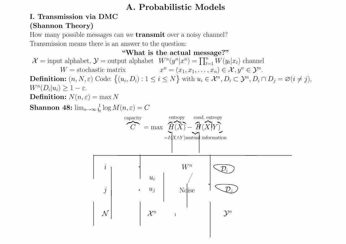
A. Probabilistic ModelsI. Transmission via DMC

(Shannon Theory)

How many possible messages can we transmit over a noisy channel?

Transmission means there is an answer to the question:

“What is the actual message?”

X = input alphabet, Y = output alphabet W n(yn|xn) =∏

n

t=1 W (yt|xt) channel

W = stochastic matrix xn = (x1, x1, . . . , xn) ∈ X , yn ∈ Yn.

Definition: (n, N, ε) Code:{(ui, Di) : 1 ≤ i ≤ N

}with ui ∈ X n, Di ⊂ Yn, Di ∩ Dj = ∅(i 6= j),

W n(Di|ui) ≥ 1 − ε.

Definition: N(n, ε) = max N

Shannon 48: limn→∞1n

log M(n, ε) = C

capacity︷︸︸︷

C = max

entropy︷ ︸︸ ︷

H(X)−cond. entropy︷ ︸︸ ︷

H(X|Y )︸ ︷︷ ︸

=I(X∧Y )mutual information

-

--

W n

Noise

i

j

ui

uj

N X n Yn

.................

.............

..........

.......

.....

.....

.......

..........

.............................

................... .........................................

..

.................

..............

...........

..

..

..

..

..

..

..

..

..

..

..

..

..

..

..

..

..

.

..

..

..

..

..

..

............

.............

.............................

..................

.....................

........................

.................

..............

..........

.......

......

....

.....

........

...........

............................. ................... .......................

....................

..................

...............

............

..........

..

..

..

..

..

..

..

.

..

..

..

..

..

..

..

..

..

..

..

..

..

..

..

............

.............

................................

....................

.......................

..........................

Di

Dj

1

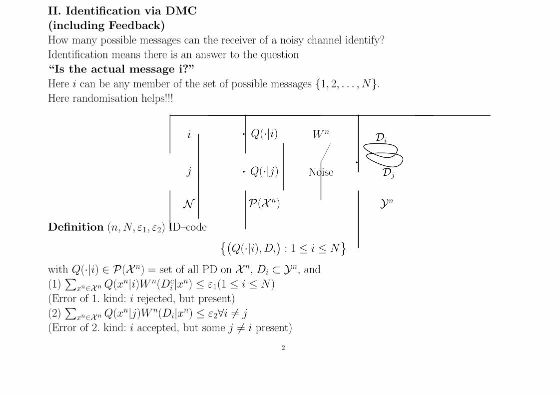
II. Identification via DMC

(including Feedback)

How many possible messages can the receiver of a noisy channel identify?

Identification means there is an answer to the question

“Is the actual message i?”

Here i can be any member of the set of possible messages {1, 2, . . . , N}.

Here randomisation helps!!!

-

--

W n

Noise

i

j

Q(·|i)

Q(·|j)

.................

.............

..........

.......

.....

.....

.......

..........

.............................

................... .........................................

..

.................

..............

...........

........

..

..

..

..

..

..

..

..

..

..

..

..

..

.

..

..

..

..

..

..

............

.............

.............................

..................

.....................

........................

.................

..............

..........

.......

......

....

.....

........

........................................ ................... ....................... ....................

..................

...............

............

..........

........

..

..

..

.

..

..

..

..

..

..

..

..

..

..

..

..

..

..

..

............

.............

................................

....................

.......................

..........................

N P(X n) Yn

Di

Dj

Definition (n, N, ε1, ε2) ID–code{(

Q(·|i), Di

): 1 ≤ i ≤ N

}

with Q(·|i) ∈ P(X n) = set of all PD on X n, Di ⊂ Yn, and

(1)∑

xn∈Xn Q(xn|i)W n(Dci |xn) ≤ ε1(1 ≤ i ≤ N)

(Error of 1. kind: i rejected, but present)

(2)∑

xn∈Xn Q(xn|j)W n(Di|xn) ≤ ε2∀i 6= j

(Error of 2. kind: i accepted, but some j 6= i present)

2

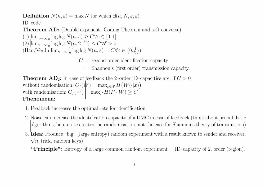
Definition N(n, ε) = max N for which ∃(n, N, ε, ε)

ID–code

Theorem AD: (Double exponent.–Coding Theorem and soft converse)

(1) limn→∞1n

log log N(n, ε) ≥ C∀ε ∈ [0, 1]

(2) limn→∞1n

log log N(n, 2−δn) ≤ C∀δ > 0.

(Han/Verdu limn→∞1n

log log N(n, ε) = C∀ε ∈(0, 1

2

))

C = second order identification capacity

= Shannon’s (first order) transmission capacity.

Theorem AD2: In case of feedback the 2–order ID–capacities are, if C > 0

without randomisation: Cf(W ) = maxx∈X H(W (·|x)

)

with randomisation: Cf(W ) = maxP H(P · W ) ≥ C

Phenomena:

1. Feedback increases the optimal rate for identification.

2. Noise can increase the identification capacity of a DMC in case of feedback (think about probabilistic

algorithms, here noise creates the randomisation, not the case for Shannon’s theory of transmission)

3. Idea: Produce “big” (large entropy) random experiment with a result known to sender and receiver.√n–trick, random keys)

“Principle”: Entropy of a large common random experiment = ID–capacity of 2. order (region).

3

Remark: ID–theory led to foundation of new areas and stimulated further research

Approximation of output distributions.

Converse for Theorem AD1

-

W

....................

..................

................

..............

............

...........

...........

...........

.............

...............

..................

.......................................... ........................

......................

...................

.................

..............

..

..

..

..

....

..

..

..

..

..

..

..

..

..

..

..

..

.

..

..

..

..

..

..

..

..

..

..

..

..

..

..

..

..

..

..

..

..

..

..

..

..

.

..

..

..

..

..

..

..

..

..

..

.

..

..

..

..

..

..

..

..

..

..

.

..

..

..

..

..

..

..

..

..

................

...............

..............

...........................

...............

................

.................

...................

......................

..........................

.......................

.....................

..................

...............

..............

.............

............

.............

................

..................

........................................... .......................

.....................

...................

.................

...............

..

..

..

.......

..

..

..

..

..

..

..

..

..

..

..

..

..

..

.

..

..

..

..

..

..

..

..

..

..

..

..

..

..

..

..

.

..

..

..

..

..

..

..

..

..

.

..

..

..

..

..

..

..

..

..

..

..

..

..

..

..

..

..

..

..

..

..

..

..

..

..

..

..

..

..

..

..

..

..

..

..

..

..

..

..

..

..

..

..

.

..

..

..

..

..

..

..

..

.

..

..

..

..

..

..

..

.............

............

........................

.............

...............

................

..................

.....................

........................

P Q = PW

How can we count?

Find U ⊂ X n with uniform distribution PU :

PU · W ∼ Q

Minimize |U|, then N .(|X n||U|).

4

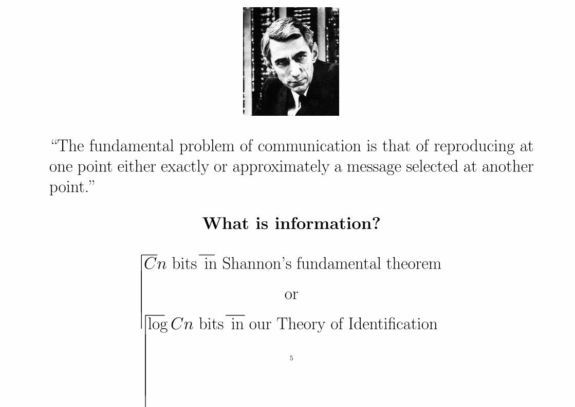
“The fundamental problem of communication is that of reproducing atone point either exactly or approximately a message selected at anotherpoint.”

What is information?

Cn bits in Shannon’s fundamental theorem

or

log Cn bits in our Theory of Identification

5

III. Discovery of

Mystery Numbers = Common Randomness Capacity

Mystery Number

In dealing with different kinds of feedback strategies it is convenient to have the following concept. Let

Fn(n = 1, 2, . . . ) be a subset of the set of all randomized feedback strategies F rn of a DMC W with

blocklength n and let it contain the set Fdn of all deterministic strategies.

We call (Fn)∞n=1 a smooth class of strategies if for all n1, n2 ∈ N and n = n1 + n2

Fn ⊃ Fn1× Fn2

(*)

where the product means concatenation of strategies.

For fn ∈ Fn the channel induces an output sequence Y n(fn). For any smooth class we define numbers

µ(Fn) = maxfn∈FnH(Y n(fn))

By (*) and the memoryless character of the channel

µ(Fn) ≥ µ(Fn1) + µ(Fn2

),

and therefore

µ = µ((Fn)∞n=1 = limn→∞ 1/nµ(Fn) exists.

It is called mystery number to attract attention.6

Common Randomness Capacity

The common randomness capacity CCR is the maximal number ν such, that for aconstant c > 0 and for all ǫ > 0, δ > 0 and for all n sufficiently large there exists apermissible pair (K, L) of random variables for length n on a set K with |K| < e

cn

with

Pr{K 6= L} < ǫ andH(K)

n> ν − δ.

7

From common randomness to identification: (now also called shared randomness)

The√

n-trick

Let [M ] = {1, 2, . . . , M}, [M ′] = {1, 2, . . . , M ′} and let T = {Ti : i = 1, . . . , N} be a family of maps

Ti : [M ] → [M ′] and consider for i = 1, 2, . . . , N the sets

Ki = {(m, Ti(m)) : m ∈ [M ]}and on [M ] × [M ′] the PD’s

Qi((m, m′)) =

1

Mfor all (m, m

′) ∈ Ki.

Lemma: Given M, M ′ = exp{√log M} and ǫ > 0 there exists a family T = T (ǫ, M) such that

• |T | = N ≥ exp{M − c(ǫ)√

n}• Qi(Ki) = 1 for i = 1, . . . , N

• Qi(Kj) ≤ ǫ ∀i 6= j

Note In typical applications the common random experiment has range M = exp{CRn} and uses for

its realisation

blocklength n

while the extension by the Ti uses

blocklength√

n

.8

Capacity Regions

Transmission Identification

DMC X X

MAC X X

BC ? X

TWC ? ?

With Feedback

DMC X X

MAC ? XD

MAC 1.) ? ?R

BC ? ?D

BC 2.) ? XR

TWC ? XD

Amazing dualities transmission versus identification:

for instance concerning feedback:

there is a rather unified theory of

Multi-user identification with feedback - with constructive solutions, whereas for

transmission with feedback most capacity regions are unknown.

9

and concerning MAC and BC:

1.) Mystery numbers for MAC?

2.) Mystery number region for BC known!

For transmission capacity regions the situation is reversed.

10

Further cases of validity of the “principle”

— Ahlswede/Zhang 1993: Cryptography (Wire tape channel)

— Ahlswede/Balakirsky (Correlated source helps)

— Ahlswede/Cai (More on AVC, correlated source helps)

— Ahlswede/Csiszar: AVC See Blackwell/Breiman/Thomasian 1960

— Ahlswede, Steinberg: MAC

— Ahlswede: BC

— Bassalygo/Burnashev ( relation to cryptography)

— Ahlswede/Csiszar: Common Randomness: its role in Information Theory and Cryptography, Part II, 1998

— This work was continued in several papers by Csiszar/Narayan

— Venkatesan/Anantharam: The common randomness capacity of a pair of independent discrete me-

moryless channels, 1998

Entropy characterisation to calculate entropy of common random experiment

Example MAC:

Xn+1 = fn+1(Zn)

Yn+1 = gn+1(Zn)

Xn Y n

Zn –common Max H(Zn)=?

(identification–transmission)11

A/Balakirsky

DMC

-

--

W n

Noise

i

j

Q(·|i)

Q(·|j)

.................

.............

..........

.......

.....

.....

.......

..........

.............................

................... ........................................

...

.................

..............

...........

........

..

..

..

..

..

..

..

..

..

..

..

..

..

.

..

..

..

..

..

..

............

.............

.............................

..................

.....................

........................

.................

..............

..........

.......

......

....

.....

........

........................................ ................... ....................... ....................

..................

...............

............

..........

..

......

..

..

..

.

..

..

..

..

..

..

..

..

..

..

..

..

..

..

..

............

.............

................................

....................

.......................

..........................

N P(X n) Yn

Di

Dj

How much does a correlated source

Un

sender sideV

n

receiver side

help for IDENTIFICATION over the DMC?

The “Principle” suggests the question:

How much does DMC help for Common Randomness in (Un, V n)?12

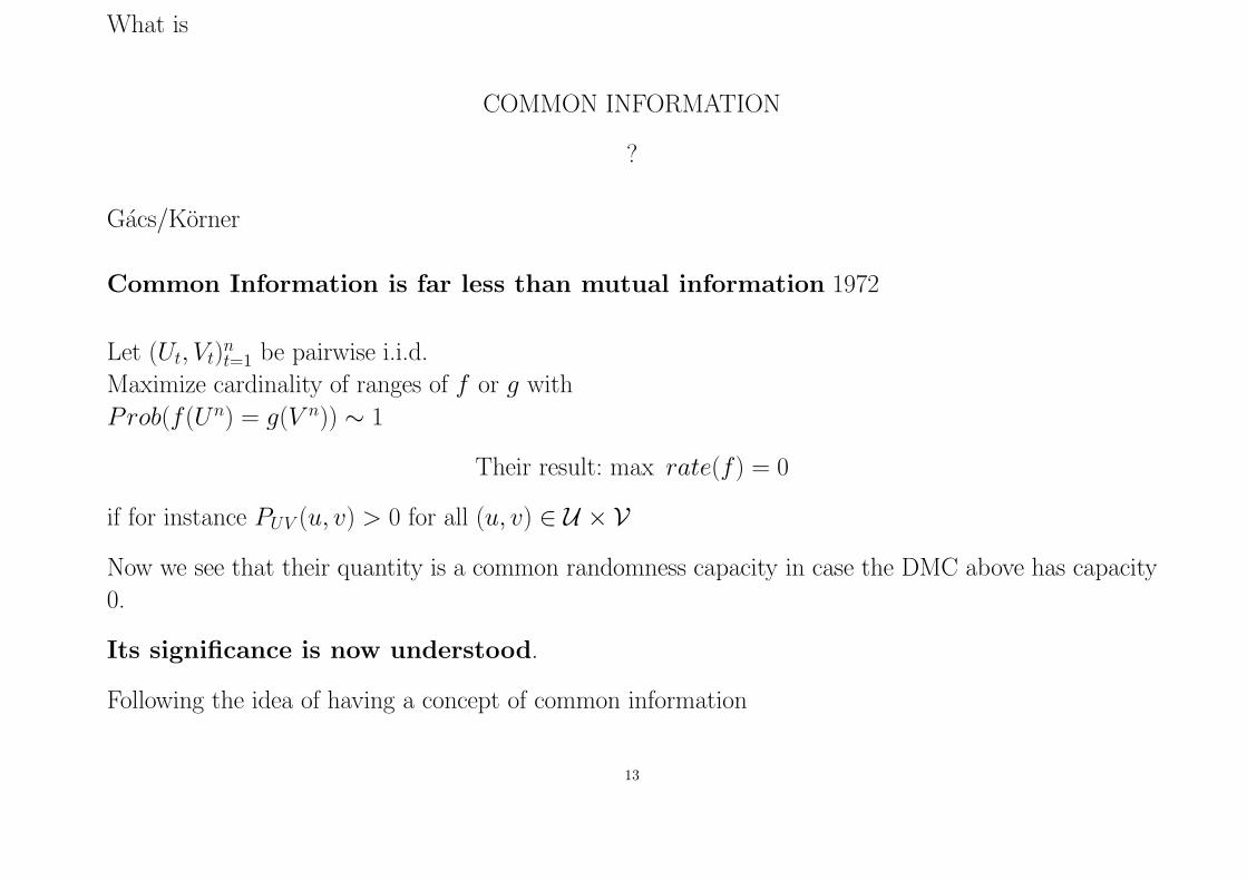
What is

COMMON INFORMATION

?

Gacs/Korner

Common Information is far less than mutual information 1972

Let (Ut, Vt)nt=1 be pairwise i.i.d.

Maximize cardinality of ranges of f or g with

Prob(f(Un) = g(V n)) ∼ 1

Their result: max rate(f) = 0

if for instance PUV (u, v) > 0 for all (u, v) ∈ U × V

Now we see that their quantity is a common randomness capacity in case the DMC above has capacity

0.

Its significance is now understood.

Following the idea of having a concept of common information

13

Wyner: Common Information

CWyner depends on probabilities not only on positivities

Claimed to have the notion of common information.

Note: CWyner(U, V ) ≥ I(U ∧ V )

14

Comparison of identification rate and common randomness capacity: Identification

rate can exceed common randomness capacity and vice versa

One of the observations was that random experiments, to whom the communicators have access, essenti-

ally influence the value of the identification capacity CI . Actually, if sender and receiver have a common

random capacity CR then by the√

n–trick always

CI ≥ CR if CI > 0.

For many channels, in particular for channels with feedback, equality has been proved.

It seemed therefore plausible, that this is always the case, and that the theory of identification is basically

understood, when common random capacities are known.

We report here a result, which shows that this expected unification is not valid in general — there

remain two theories.

Example: CI = 1, CR = 0. (Fundamental)

(Kleinewachter found also an example involving feedback with 0 < CI < CR)

We use a Gilbert type construction of error correcting codes with constant weight words. This was done

for certain parameters. The same arguments give for parameters needed here the following auxiliary

result.

Proposition. Let Z be a finite set and let λ ∈ (0, 1/2) be given. For ε < (22/λ + 1)−1 a family

A1, . . . , AN of subsets of Z exists with the properties

|Ai| = ε|Z|, |Ai ∩ Aj| < λε|Z| (i 6= j)

and

N ≥ |Z|−12⌊ε|Z|⌋ − 1.15

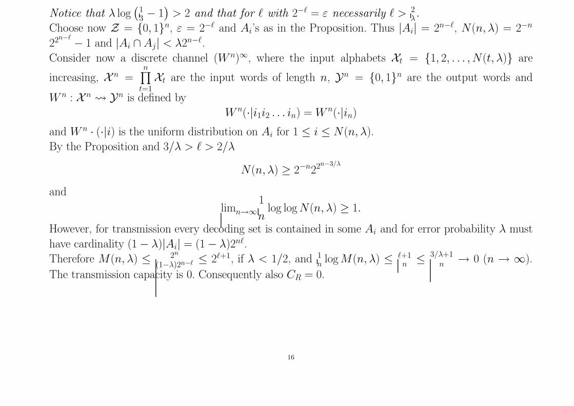
Notice that λ log(

13 − 1

)> 2 and that for ℓ with 2−ℓ = ε necessarily ℓ >

2λ.

Choose now Z = {0, 1}n, ε = 2−ℓ and Ai’s as in the Proposition. Thus |Ai| = 2n−ℓ, N(n, λ) = 2−n

22n−ℓ − 1 and |Ai ∩ Aj| < λ2n−ℓ.

Consider now a discrete channel (W n)∞, where the input alphabets Xt = {1, 2, . . . , N(t, λ)} are

increasing, X n =n∏

t=1Xt are the input words of length n, Yn = {0, 1}n are the output words and

W n : X n Yn is defined by

Wn(·|i1i2 . . . in) = W

n(·|in)and W n · (·|i) is the uniform distribution on Ai for 1 ≤ i ≤ N(n, λ).

By the Proposition and 3/λ > ℓ > 2/λ

N(n, λ) ≥ 2−n22n−3/λ

and

limn→∞1

nlog log N(n, λ) ≥ 1.

However, for transmission every decoding set is contained in some Ai and for error probability λ must

have cardinality (1 − λ)|Ai| = (1 − λ)2nℓ.

Therefore M(n, λ) ≤ 2n

(1−λ)2n−ℓ≤ 2ℓ+1, if λ < 1/2, and 1

nlog M(n, λ) ≤ ℓ+1

n≤ 3/λ+1

n→ 0 (n → ∞).

The transmission capacity is 0. Consequently also CR = 0.

16

IV. “Consequences” for Secrecy Systems

Characterisation of the capacity region for the BC for identification

We need the direct part of the ABC Coding Theorem for transmission.

(Cover, van der Meulen; Korner and Marton)

Here, there are separate messages for decoder Y (resp. Z) and common messages for both decoders.

Achievable are (with maximal errors)

TY ={(RY , R0) : R0 ≤ I(U ∧ Z), R0 + RY

≤ min[I(X ∧ Y ), I(X ∧ Y |U) + I(U ∧ Z)

],

U X Y Z, ‖U‖ ≤ |X | + 2}

resp. TZ ={(R0, RZ) : R0 ≤ I(U ∧ Y ), R0 + RZ

≤ min[I(X ∧ Z), I(X ∧ Z|U) + I(U ∧ Y )

],

U X Y Z, ‖U‖ ≤ |X | + 2}.

This is our surprising result.

Theorem: For the (general) BC the set of achievable pairs of second order rates for identification

is given by

B = T ′Y ∪ T ′

Z ,

where

T ′Y = {(R′

Y, R′Z) : ∃(RY, R0) ∈ TY with R

′Y = RY + R0, R

′Z = R0} and

T ′Z = {(R′

Y , R′Z) : ∃(R0, RZ) ∈ TZ with R

′Y = R0, R

′Z = R0 + RZ}.

Remark: B gives also the achievable pairs of first order rates for common randomness. Proof goes via identification!17

Transmission, identification and common randomness capacities for wire-tape

channels with secure feedback from the decoder

R. Ahlswede and N. Cai

Problems on General Theory of Information Transfer, particularly,

transmission, identification and common randomness, via a wire-tap channel with

secure feedback

are studied in this work.

Wire-tap channels were introduced by A. D. Wyner and

were generalized by I. Csiszar and J. Korner.

Its identification capacity was determined by R. Ahlswede and Z. Zhang.

Here by secure feedback we mean that the feedback is noiseless and that the wire-tapper has no knowledge

about the content of the feedback except via his own output.

Lower and upper bounds to the transmission capacity are derived. The two bounds are shown

to coincide for two families of degraded wire-tap channels, including Wyner’s original version of the

wire-tap channel.

The identification and common randomness capacities for the channels are completely determi-

ned.

Also here again identification capacity is much bigger than common randomness ca-

pacity, because the common randomness used for the (secured) identification needs not to be secured!

18

V. More General Transfer Models

Our work on identification has led us to reconsider the basic assumptions of Shannon’s Theory. It deals

with “messages”, which are elements of a prescribed set of objects, known to the communicators.

The receiver wants to know the true message. This basic model occuring in all engineering work on

communication channels and networks addresses a very special communication situation. More generally

they are characterized by

(I) The questions of the receivers concerning the given “ensemble”, to be answered by the sender(s)

(II) The prior knowledge of the receivers

(III) The senders prior knowledge.

It seems that the whole body of present day Information Theory will undergo serious revisions and

some dramatic expansions. We open several directions of future research and start the mathematical

description of communication models in great generality. For some specific problems we provide solutions

or ideas for their solutions.

One sender answering several questions of receivers

A general communication model for one sender

To simplify matters we assume first that the noise is modelled by a discrete memoryless channel (DMC)

with input (resp. output) alphabet X (resp. Y) and transmission matrix W .

19

The goal in the classical Shannon communication theory is to transmit many messages reliably over this

channel. This is done by coding. An (n, M, λ)–code is a system of pairs{(ui, Di) : 1 ≤ i ≤ M

}with

ui ⊂ X n, Di ⊂ Yn and

Di ∩ Di′ = ∅ for i = 1, . . . , M,

W (Dc

i |ui) ≤ λ for i = 1, . . . , M.

Given a set of messages M = {1, . . . , M}, by assigning i to codeword ui we can transmit a message

from M in blocklength n over the channel with a maximal error probability less than λ. Notice that

the underlying assumption in this classical transmission problem is that both, sender and receiver, know

that the message is from a specified set M. They also know the code. The receiver’s goal is to get

to know the message sent.

One can conceive of many situations in which the receiver has (or many receivers have) different

goals.

A nice class of such situations can, abstractly, be described by a family Π(M) of partitions of M.

Decoder π ∈ Π(M) wants to know only which member of the partition π = (A1, . . . , Ar) contains m,

the true message, which is known to the encoder.

We describe now some seemingly natural families of partitions.

Model 1: ΠS = {πsh}, πsh ={{m} : m ∈ M

}. This describes Shannon’s classical transmission

problem stated above.

Model 2: ΠI = {πm : m ∈ M} with πm ={{m},M r {m}

}. Here decoder πm wants to know

whether m occured or not. This is the identification problem.

20

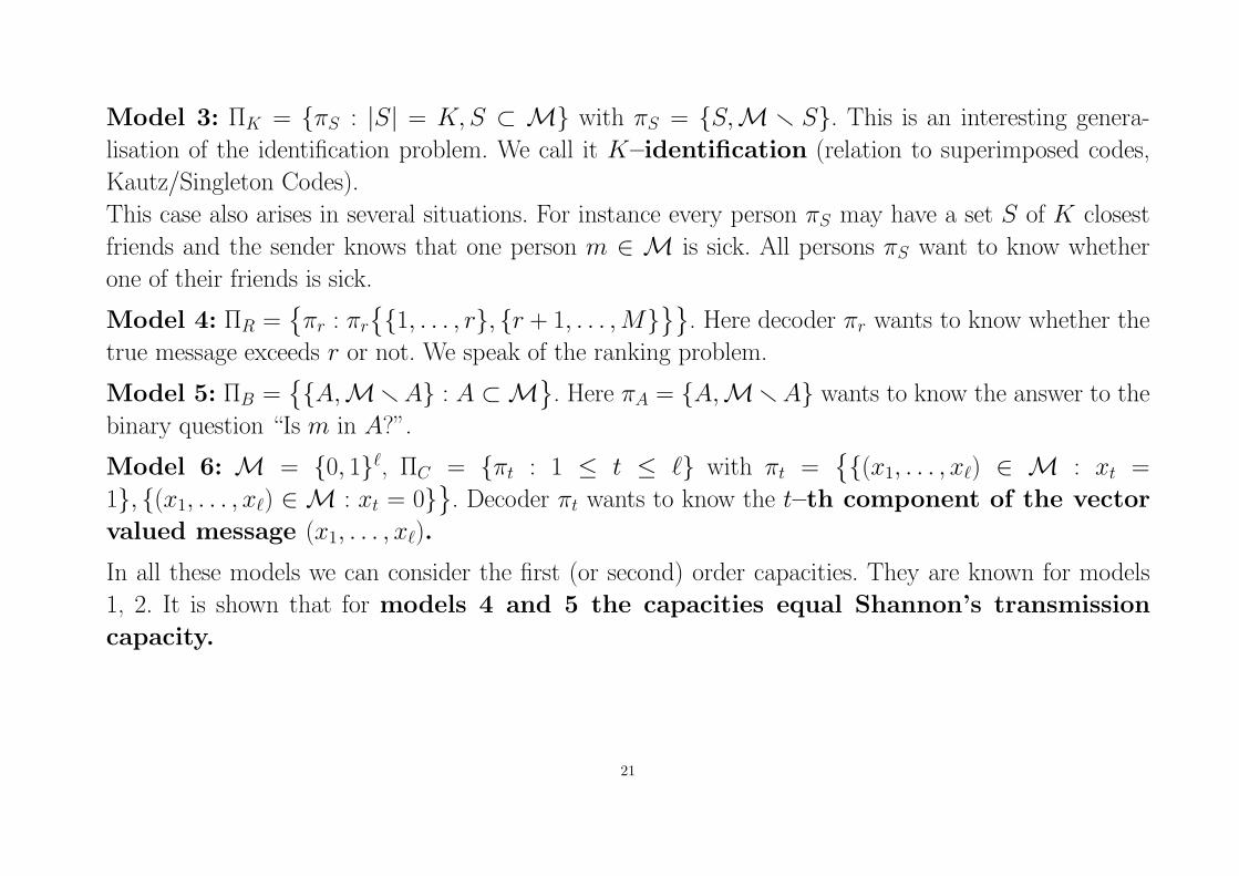
Model 3: ΠK = {πS : |S| = K, S ⊂ M} with πS = {S,M r S}. This is an interesting genera-

lisation of the identification problem. We call it K–identification (relation to superimposed codes,

Kautz/Singleton Codes).

This case also arises in several situations. For instance every person πS may have a set S of K closest

friends and the sender knows that one person m ∈ M is sick. All persons πS want to know whether

one of their friends is sick.

Model 4: ΠR ={πr : πr

{{1, . . . , r}, {r + 1, . . . , M}

}}. Here decoder πr wants to know whether the

true message exceeds r or not. We speak of the ranking problem.

Model 5: ΠB ={{A,Mr A} : A ⊂ M

}. Here πA = {A,Mr A} wants to know the answer to the

binary question “Is m in A?”.

Model 6: M = {0, 1}ℓ, ΠC = {πt : 1 ≤ t ≤ ℓ} with πt ={{(x1, . . . , xℓ) ∈ M : xt =

1}, {(x1, . . . , xℓ) ∈ M : xt = 0}}. Decoder πt wants to know the t–th component of the vector

valued message (x1, . . . , xℓ).

In all these models we can consider the first (or second) order capacities. They are known for models

1, 2. It is shown that for models 4 and 5 the capacities equal Shannon’s transmission

capacity.

21

The most challenging problem is the general K-identification problem of model 3. Here

an (n, N, K, λ)–code is a family of pairs{(Q(·|i), Dπ) : 1 ≤ i ≤ N, π ∈ ΠK

}, where the Q(·|i)’s are

PD’s on X n, Dπ ⊂ Yn, and where for all π = {S,M r S}(

S ∈(M

K

))

∑

xn

Q(xn|i)W (Dc

π|xn) ≤ λ for all i ∈ S,

∑

xn

Q(xn|i)W (Dπ|xn) ≤ λ for all i /∈ S.

We also write DS instead of Dπ. A coding theorem is established.

Remark 1: Most models fall into the following category of regular transfer models. By this we mean

that the set of partitions Π of M is invariant under all permutations σ : M → M:

π = (A1, . . . , Ar) ∈ Π implies σπ =(σ(A1), . . . , σ(Ar)

)∈ Π.

Remark 2: Many of the models introduced concern bivariate partitions. More generally they are

described by a hypergraph H = (M, E), where decoder E wants to know whether the m occured is in

E or not.

22

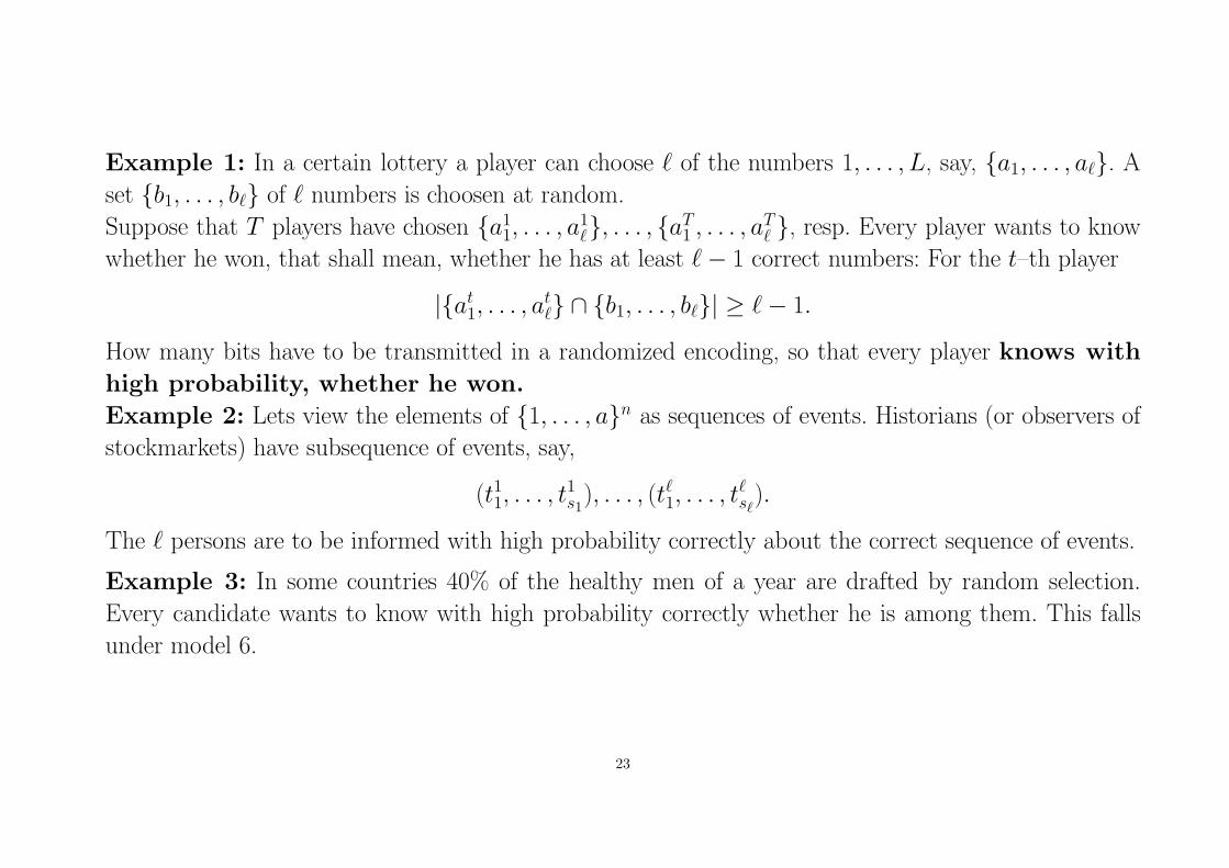
Example 1: In a certain lottery a player can choose ℓ of the numbers 1, . . . , L, say, {a1, . . . , aℓ}. A

set {b1, . . . , bℓ} of ℓ numbers is choosen at random.

Suppose that T players have chosen {a11, . . . , a

1ℓ}, . . . , {aT

1 , . . . , aT

ℓ}, resp. Every player wants to know

whether he won, that shall mean, whether he has at least ℓ − 1 correct numbers: For the t–th player

|{at

1, . . . , at

ℓ} ∩ {b1, . . . , bℓ}| ≥ ℓ − 1.

How many bits have to be transmitted in a randomized encoding, so that every player knows with

high probability, whether he won.

Example 2: Lets view the elements of {1, . . . , a}n as sequences of events. Historians (or observers of

stockmarkets) have subsequence of events, say,

(t11, . . . , t1s1

), . . . , (tℓ1, . . . , tℓ

sℓ).

The ℓ persons are to be informed with high probability correctly about the correct sequence of events.

Example 3: In some countries 40% of the healthy men of a year are drafted by random selection.

Every candidate wants to know with high probability correctly whether he is among them. This falls

under model 6.

23

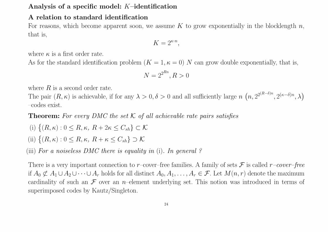
Analysis of a specific model: K–identification

A relation to standard identification

For reasons, which become apparent soon, we assume K to grow exponentially in the blocklength n,

that is,

K = 2κ·n,

where κ is a first order rate.

As for the standard identification problem (K = 1, κ = 0) N can grow double exponentially, that is,

N = 22Rn

, R > 0

where R is a second order rate.

The pair (R, κ) is achievable, if for any λ > 0, δ > 0 and all sufficiently large n(n, 22(R−δ)n

, 2(κ−δ)n, λ)

–codes exist.

Theorem: For every DMC the set K of all achievable rate pairs satisfies

(i){(R, κ) : 0 ≤ R, κ, R + 2κ ≤ Csh} ⊂ K

(ii){(R, κ) : 0 ≤ R, κ, R + κ ≤ Csh} ⊃ K

(iii) For a noiseless DMC there is equality in (i). In general ?

There is a very important connection to r–cover–free families. A family of sets F is called r–cover–free

if A0 6⊂ A1 ∪A2 ∪ · · ·∪Ar holds for all distinct A0, A1, . . . , Ar ∈ F . Let M(n, r) denote the maximum

cardinality of such an F over an n–element underlying set. This notion was introduced in terms of

superimposed codes by Kautz/Singleton.

24

VI. Extensions to Classical/Quantum Channels

Great progress in recent years with fruitful exchanges between Information Theory andPhysics.

Note: Common Randomness — Entanglement

Since I cannot expect that many listeners understand this just give classical me-thods which extend or have analoga.

25

The elimination techniqueThis method was introduced by us in 1978.

It is a general method to obtain from a correlated code for AVC with probability

λn ≤ e−ǫn

, ǫ > 0,

an ordinary code of essentially the same rate and average error probability

λn = o(1).

Since for correlated codes the capacity is known, we thus obtain the ordenary capacity.

We obtain this result, if the ordinary capacity is known to be positive.

Capacity of Quantum Arbitrarily Varying Channels

Rudolf Ahlswede and Vladimir Blinovsky

We prove that the average error capacity Cq of a quantum arbitrarily varying channel (QAVC) equals

0 or else the random code capacity C (Ahlswede’s dichotomy).

We also establish a necessary and sufficient condition for Cq > 0.

26

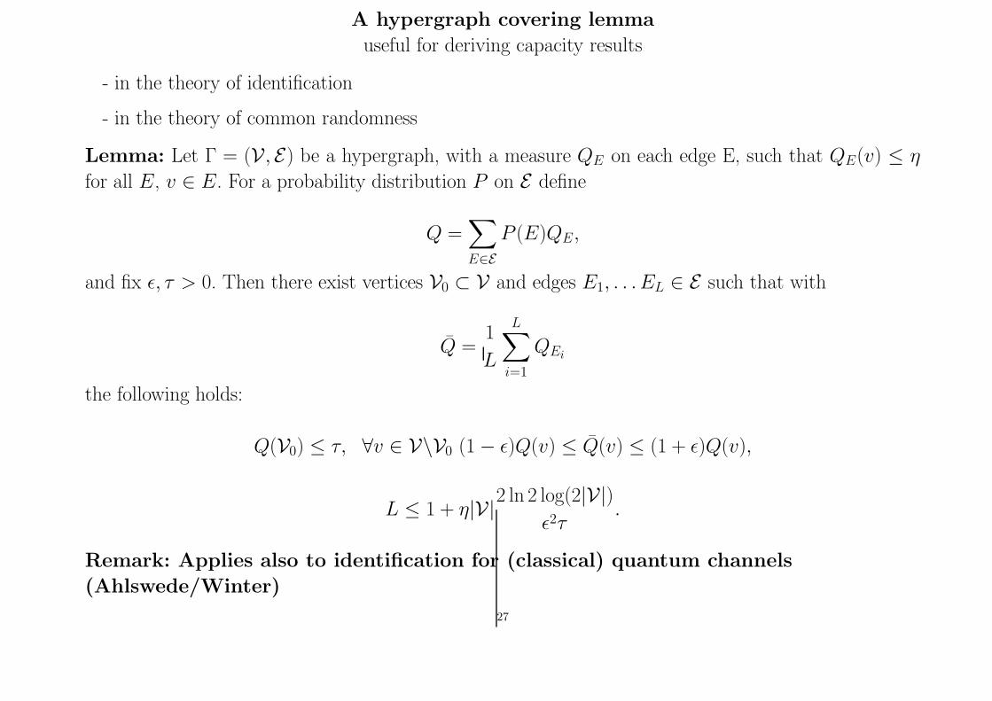
A hypergraph covering lemma

useful for deriving capacity results

- in the theory of identification

- in the theory of common randomness

Lemma: Let Γ = (V , E) be a hypergraph, with a measure QE on each edge E, such that QE(v) ≤ η

for all E, v ∈ E. For a probability distribution P on E define

Q =∑

E∈EP (E)QE,

and fix ǫ, τ > 0. Then there exist vertices V0 ⊂ V and edges E1, . . . EL ∈ E such that with

Q =1

L

L∑

i=1

QEi

the following holds:

Q(V0) ≤ τ, ∀v ∈ V\V0 (1 − ǫ)Q(v) ≤ Q(v) ≤ (1 + ǫ)Q(v),

L ≤ 1 + η|V|2 ln 2 log(2|V|)ǫ2τ

.

Remark: Applies also to identification for (classical) quantum channels

(Ahlswede/Winter)

27

The blowing up technique

We define the k–Hamming–neighbourhood ΓkB of a set B ⊂ Yn as

ΓkB , {yn ∈ Yn : d(yn

, xn) ≤ k for some y

′n ∈ B}where d(yn, y′n) , ({t : 1 ≤ t ≤ n, y′t 6= yt})

Blowing up Lemma (Ahlswede/Gacs/Korner, 1976)

For any DMC W there is a constant c(W ):

∀xn ∈ X n, B ⊂ Yn

W n(ΓkB|xn) ≥ Φ(Φ−1(W n(B|xn))) + n−1/2(k − 1)c

if Φ(t) =∫

t

−∞(2π)−1/2e−u2/2du.

Have no quantum version!

28

A wringing technique

useful for

- strong converse for multi-user channels

- converses for multiple-descriptions in rate-distortion theory

Lemma: Let P and Q be probability distributions on X n such that for a positive constant c

(1) P (xn) = (1 + c)Q(xn) for all xn ∈ X n,

then for any 0 < γ < c, 0 ≤ ǫ < 1 there exist t1, . . . , tk ∈ {1, . . . , n}, where 0 ≤ k ≤ c

γ, such that for

some xt1, . . . , xtk

(2) P (xt1|xt1

, . . . , xtk) ≤ max((1 + γ)Q(xi|xt1

, . . . , xtk), ǫ) for all xt ∈ X and all t = 1, 2, . . . , n

and

(3) P (xt1, . . . , xtk

) ≥ ǫk

Remark: Presently only method to prove strong converse for transmission for (classical) quantum

multiple-access channel (Ahlswede/Cai).

29

VII. Source Coding for Identification: a Discovery of Identification Entropy

Shannon’s Channel Coding Theorem for Transmission is paralleled by a Channel Coding Theorem for

Identification. We introduced noiseless source coding for identification and suggested the study of several

performance measures.

Interesting observations were made already for uniform sources

PN =(

1N

, . . . ,1N

), for which the worst case expected number of checkings L(PN) is approximately 2.

Actually it has been shown that

limN→∞

L(PN) = 2.

Recall that in channel coding going from transmission to identification leads from an exponentially

growing number of managable messages to double exponentially many.

Now in source coding roughly speaking the range of average code lengths for data compression is the

interval [0,∞) and it is [0, 2) for an average expected length of optimal identification procedures.

Note that no randomization has to be used here.

30

A discovery is an identification entropy, namely the functional

HI(P ) = 2

(

1 −N∑

u=1

P2u

)

(1.1)

for the source (U , P ), where U = {1, 2, . . . , N} and P = (P1, . . . , PN) is a probability distribution.

Its operational significance in identification source coding is similar to that of classical entropy H(P ) in

noiseless coding of data: it serves as a good bound.

31

Noiseless identification for sources and basic concept of performance

For the source (U , P ) let C = {c1, . . . , cN} be a binary prefix code (PC) with ‖cu‖ as length of cu.

Introduce the RV U with Prob(U = u) = Pu for u ∈ U and the RV C with C = cu = (cu1, cu2, . . . , cu‖u‖)if U = u.

We use the PC for noiseless identification, that is user u wants to know whether the

source output equals u, that is, whether C equals cu or not.

He iteratively checks whether C = (C1, C2, . . . ) coincides with cu in the first, second

etc. letter and stops when the first different letters occur or when C = cu. What is

the expected number LC(P, u) of checkings?

Related quantities are

LC = max1≤u≤N

LC(P, u), (1.2)

that is, the expected number of ckeckings for a person in the worst case, if code C is used,

L(P ) = minC

LC(P ), (1.3)

the expected number of checkings in the worst case for the best code, and finally, if users are chosen

by a RV V independent of U and defined by Prob(V = v) = Qv for v ∈ V = U , we consider

32

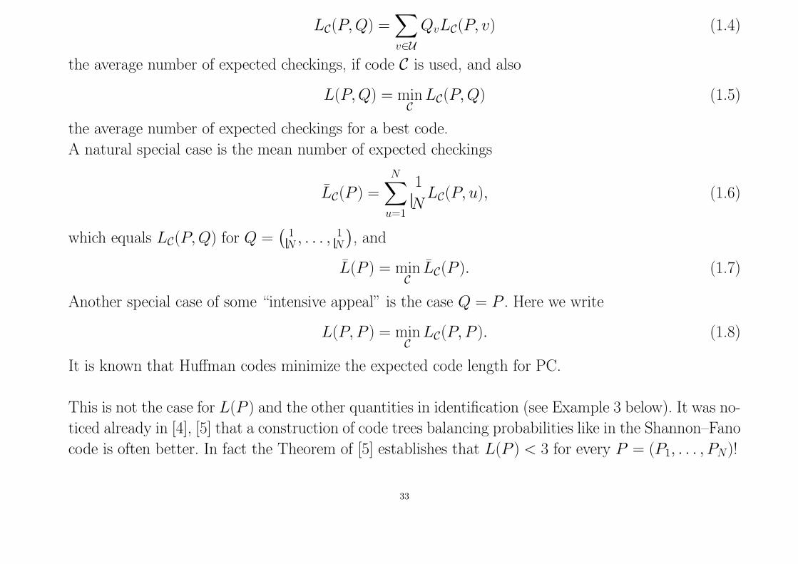
LC(P, Q) =∑

v∈UQvLC(P, v) (1.4)

the average number of expected checkings, if code C is used, and also

L(P, Q) = minC

LC(P, Q) (1.5)

the average number of expected checkings for a best code.

A natural special case is the mean number of expected checkings

LC(P ) =N∑

u=1

1

NLC(P, u), (1.6)

which equals LC(P, Q) for Q =(

1N

, . . . ,1N

), and

L(P ) = minC

LC(P ). (1.7)

Another special case of some “intensive appeal” is the case Q = P . Here we write

L(P, P ) = minC

LC(P, P ). (1.8)

It is known that Huffman codes minimize the expected code length for PC.

This is not the case for L(P ) and the other quantities in identification (see Example 3 below). It was no-

ticed already in [4], [5] that a construction of code trees balancing probabilities like in the Shannon–Fano

code is often better. In fact the Theorem of [5] establishes that L(P ) < 3 for every P = (P1, . . . , PN)!

33

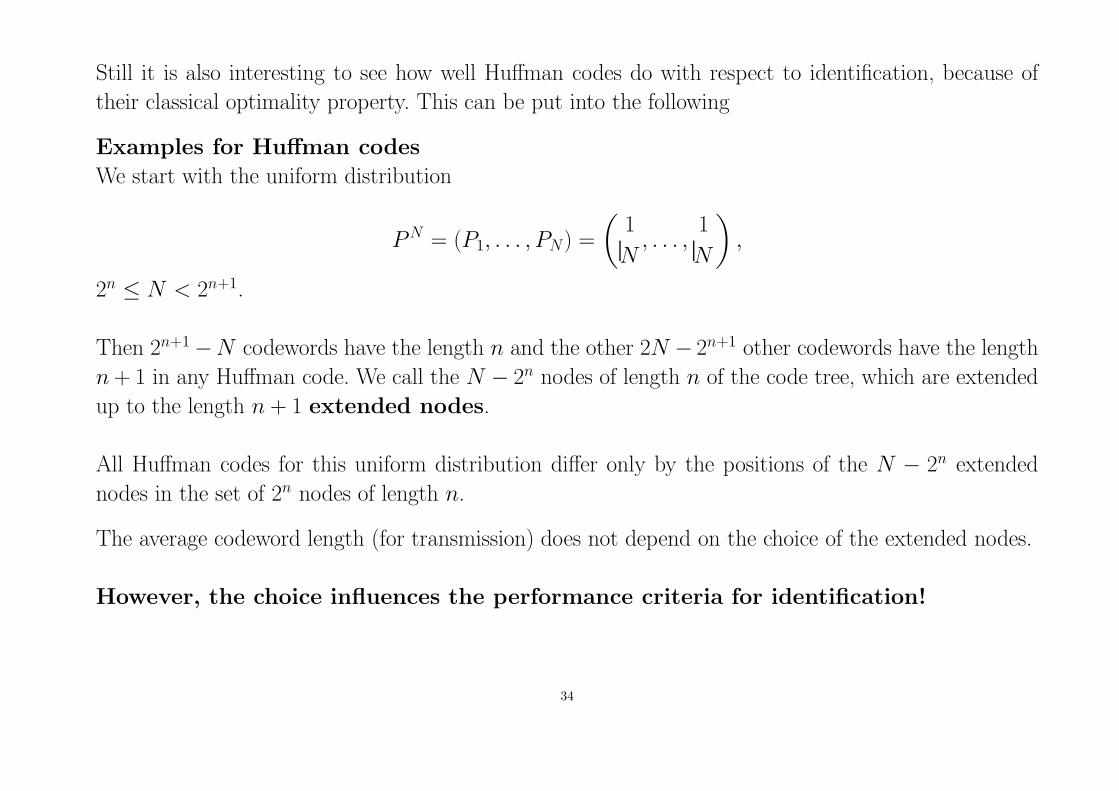
Still it is also interesting to see how well Huffman codes do with respect to identification, because of

their classical optimality property. This can be put into the following

Examples for Huffman codes

We start with the uniform distribution

PN = (P1, . . . , PN) =

(1

N, . . . ,

1

N

)

,

2n ≤ N < 2n+1.

Then 2n+1 −N codewords have the length n and the other 2N − 2n+1 other codewords have the length

n + 1 in any Huffman code. We call the N − 2n nodes of length n of the code tree, which are extended

up to the length n + 1 extended nodes.

All Huffman codes for this uniform distribution differ only by the positions of the N − 2n extended

nodes in the set of 2n nodes of length n.

The average codeword length (for transmission) does not depend on the choice of the extended nodes.

However, the choice influences the performance criteria for identification!

34

Example 1: N = 9, U = {1, 2, . . . , 9}, P1 = · · · = P9 = 19.

19 c9

19 c8

19 c1

19 c2

19 c3

19 c4

19 c5

19 c6

19 c7

29

29

29

29

39

49

59

1

Here LC(P ) ≈ 2.111, LC(P, P ) ≈ 1.815 because

LC(P ) = LC(c8) =4

9· 1 +

2

9· 2 +

1

9· 3 +

2

9· 4 = 2

1

9

LC(c9) = LC(c8), LC(c7) = 18

9, LC(c5) = LC(c6) = 1

7

9,

LC(c1) = LC(c2) = LC(c3) = LC(c4) = 16

9and therefore

35

LC(P, P ) =1

9

[

16

9· 4 + 1

7

9· 2 + 1

8

9· 1 + 2

1

9· 2

]

= 122

27= LC,

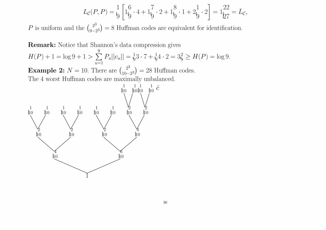
P is uniform and the(

23

9−23

)= 8 Huffman codes are equivalent for identification.

Remark: Notice that Shannon’s data compression gives

H(P ) + 1 = log 9 + 1 >

9∑

u=1Pu||cu|| = 1

93 · 7 + 1

94 · 2 = 32

9≥ H(P ) = log 9.

Example 2: N = 10. There are(

23

10−23

)= 28 Huffman codes.

The 4 worst Huffman codes are maximally unbalanced.110 c

110

110

110

110

110

110

110

110

110

210

210

210

210

210

410

410

610

1

36

Here LC(P ) = 2.2 and LC(P, P ) = 1.880, because

LC(P ) = 1 + 0.6 + 0.4 + 0.2 = 2.2

LC(P, P ) =1

10[1.6 · 4 + 1.8 · 2 + 2.2 · 4] = 1.880.

One of the 16 best Huffman codes

110

c110

110

110

210

110

110

110

110

110

110

210

310

210

210

310

510

510

1

Here LC(P ) = 2.0 and LC(P, P ) = 1.840 because

LC(P ) = LC(c) = 1 + 0.5 + 0.3 + 0.2 = 2.000

LC(P, P ) =1

5(1.7 · 2 + 1.8 · 1 + 2.0 · 2) = 1.840

37

Theorem: For every source (U , P N)

L(P N) ≥ L(P N, P

N) ≥ HI(PN).

Theorem: For P N = (P1, . . . , PN)

L(P N) ≤ 2

(

1 − 1

N2

)

.

Theorem: For P N = (2−ℓ1, . . . , 2−ℓN ) with 2-powers as probabilities

L(P N, P

N) = HI(PN).

Theorem:

L(P N, P

N) ≤ 2

1 −∑

u

α(u)∑

s=1

P2us

≤ 2

(

1 − 1

2

∑

u

P2u

)

.

For Pu = 1N

(u ∈ U) this gives the upper bound 2(1 − 1

2N

), which is better than the bound 2

(1 − 1

N2

)

for uniform distributions.

Finally we derive

Corollary.

L(P N, P

N) ≤ HI(PN) + max

1≤u≤N

Pu.

It shows the lower bound of L(P n, P N) by HI(PN) and this upper bound are close.

38

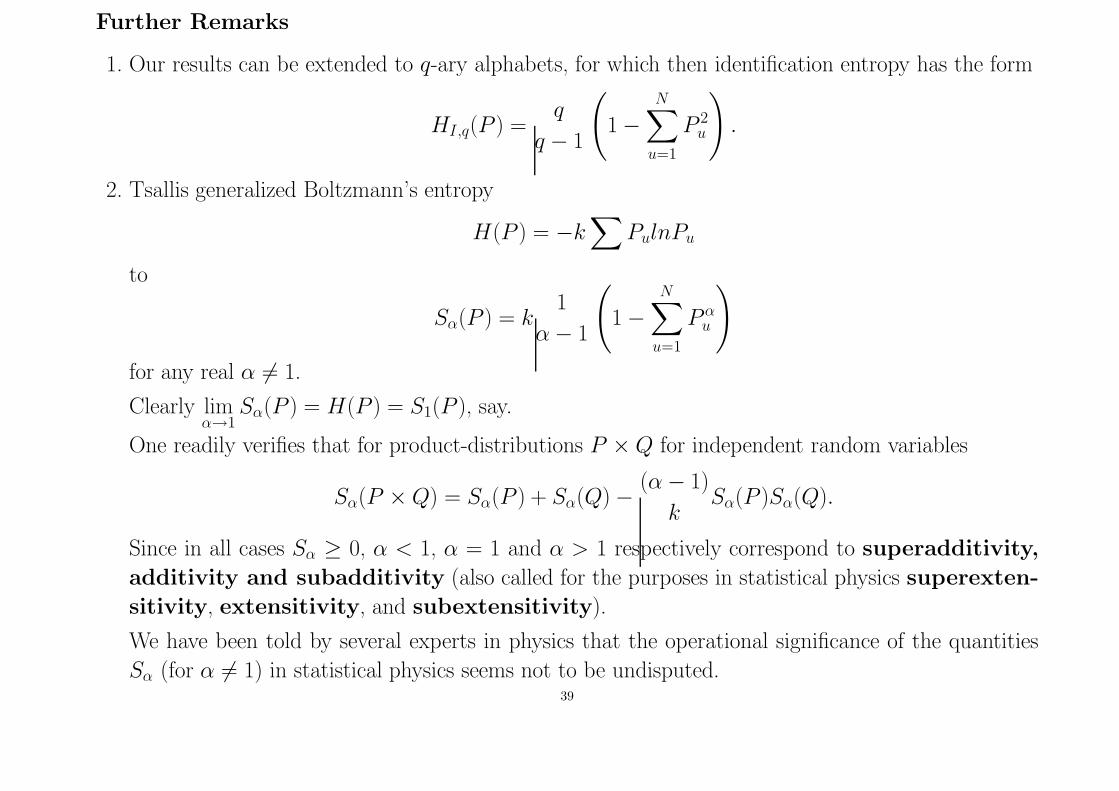
Further Remarks

1. Our results can be extended to q-ary alphabets, for which then identification entropy has the form

HI,q(P ) =q

q − 1

(

1 −N∑

u=1

P2u

)

.

2. Tsallis generalized Boltzmann’s entropy

H(P ) = −k

∑

PulnPu

to

Sα(P ) = k1

α − 1

(

1 −N∑

u=1

Pα

u

)

for any real α 6= 1.

Clearly limα→1

Sα(P ) = H(P ) = S1(P ), say.

One readily verifies that for product-distributions P × Q for independent random variables

Sα(P × Q) = Sα(P ) + Sα(Q) − (α − 1)

kSα(P )Sα(Q).

Since in all cases Sα ≥ 0, α < 1, α = 1 and α > 1 respectively correspond to superadditivity,

additivity and subadditivity (also called for the purposes in statistical physics superexten-

sitivity, extensitivity, and subextensitivity).

We have been told by several experts in physics that the operational significance of the quantities

Sα (for α 6= 1) in statistical physics seems not to be undisputed.39

In contrast we have demonstrated the significance of identification entropy, which is

formally close, but essentially different for two reasons: always α = 2 and k = q

q−1 is uniquely

determined and depends on the alphabet size q!

40

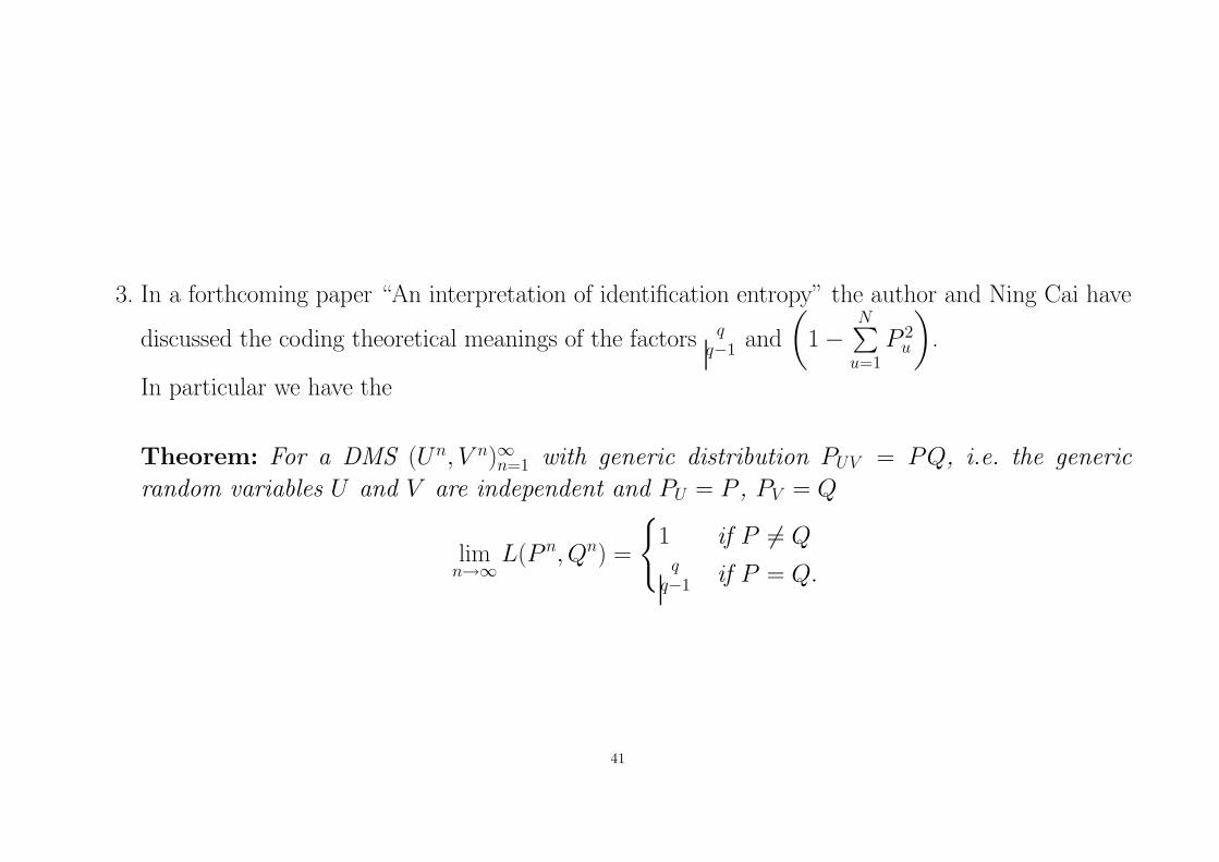
3. In a forthcoming paper “An interpretation of identification entropy” the author and Ning Cai have

discussed the coding theoretical meanings of the factors q

q−1 and

(

1 −N∑

u=1P 2

u

)

.

In particular we have the

Theorem: For a DMS (Un, V n)∞n=1 with generic distribution PUV = PQ, i.e. the generic

random variables U and V are independent and PU = P , PV = Q

limn→∞

L(P n, Q

n) =

{

1 if P 6= Q

q

q−1if P = Q.

41

B. Combinatorial Models

That Combinatorics

and Information Sciences

often come together is no surprise

they were born as twins

(Leibniz Ars Combinatoria gives credit to

Raimundus Lullus from Catalania,

who wanted to create a formal

language).

42

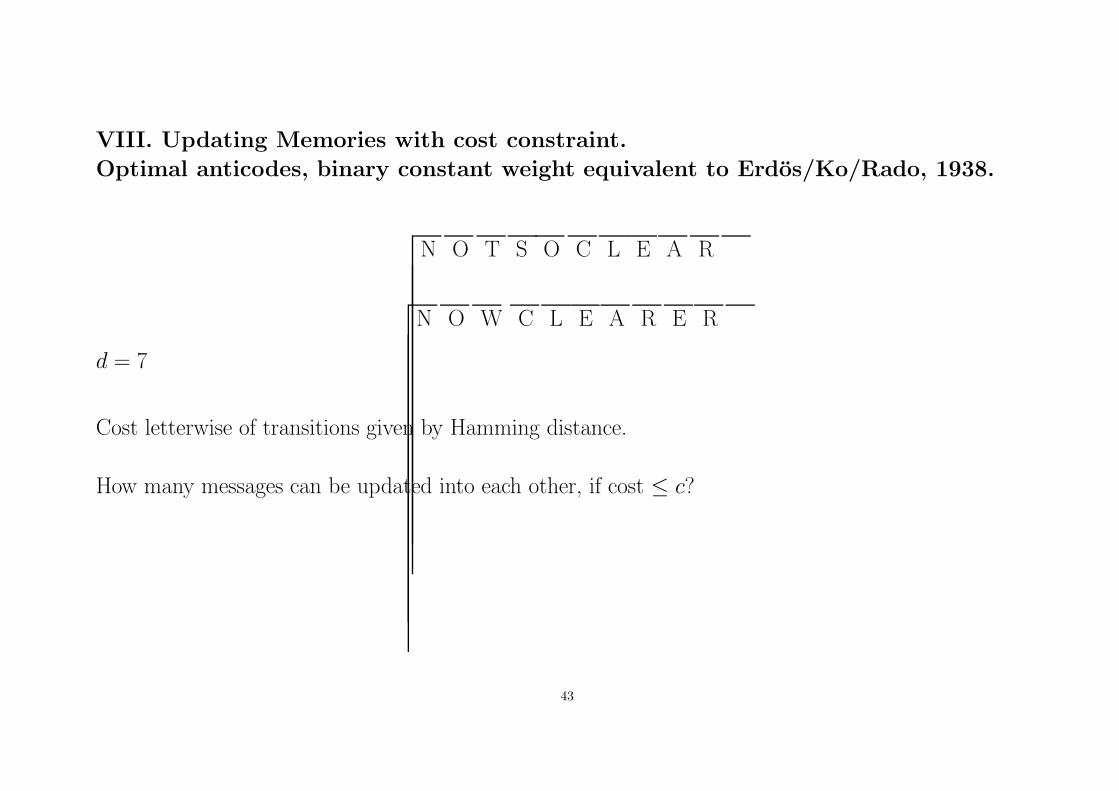
VIII. Updating Memories with cost constraint.

Optimal anticodes, binary constant weight equivalent to Erdos/Ko/Rado, 1938.

N O T S O C L E A R

N O W C L E A R E R

d = 7

Cost letterwise of transitions given by Hamming distance.

How many messages can be updated into each other, if cost ≤ c?

43

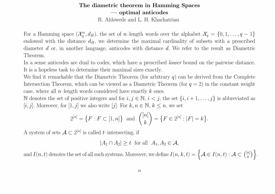
The diametric theorem in Hamming Spaces

— optimal anticodes

R. Ahlswede and L. H. Khachatrian

For a Hamming space (X nq , dH), the set of n–length words over the alphabet Xq = {0, 1, . . . , q − 1}

endowed with the distance dH , we determine the maximal cardinality of subsets with a prescribed

diameter d or, in another language, anticodes with distance d. We refer to the result as Diametric

Theorem.

In a sense anticodes are dual to codes, which have a prescribed lower bound on the pairwise distance.

It is a hopeless task to determine their maximal sizes exactly.

We find it remarkable that the Diametric Theorem (for arbitrary q) can be derived from the Complete

Intersection Theorem, which can be viewed as a Diametric Theorem (for q = 2) in the constant weight

case, where all n–length words considered have exactly k ones.

N denotes the set of positive integers and for i, j ∈ N, i < j, the set {i, i + 1, . . . , j} is abbreviated as

[i, j]. Moreover, for [1, j] we also write [j]. For k, n ∈ N, k ≤ n, we set

2[n] ={F : F ⊂ [1, n]

}and

([n]

k

)

={F ∈ 2[n] : |F | = k

}.

A system of sets A ⊂ 2[n] is called t–intersecting, if

|A1 ∩ A2| ≥ t for all A1, A2 ∈ A,

and I(n, t) denotes the set of all such systems. Moreover, we define I(n, k, t) ={

A ∈ I(n, t) : A ⊂(

[n]k

)}

.

44

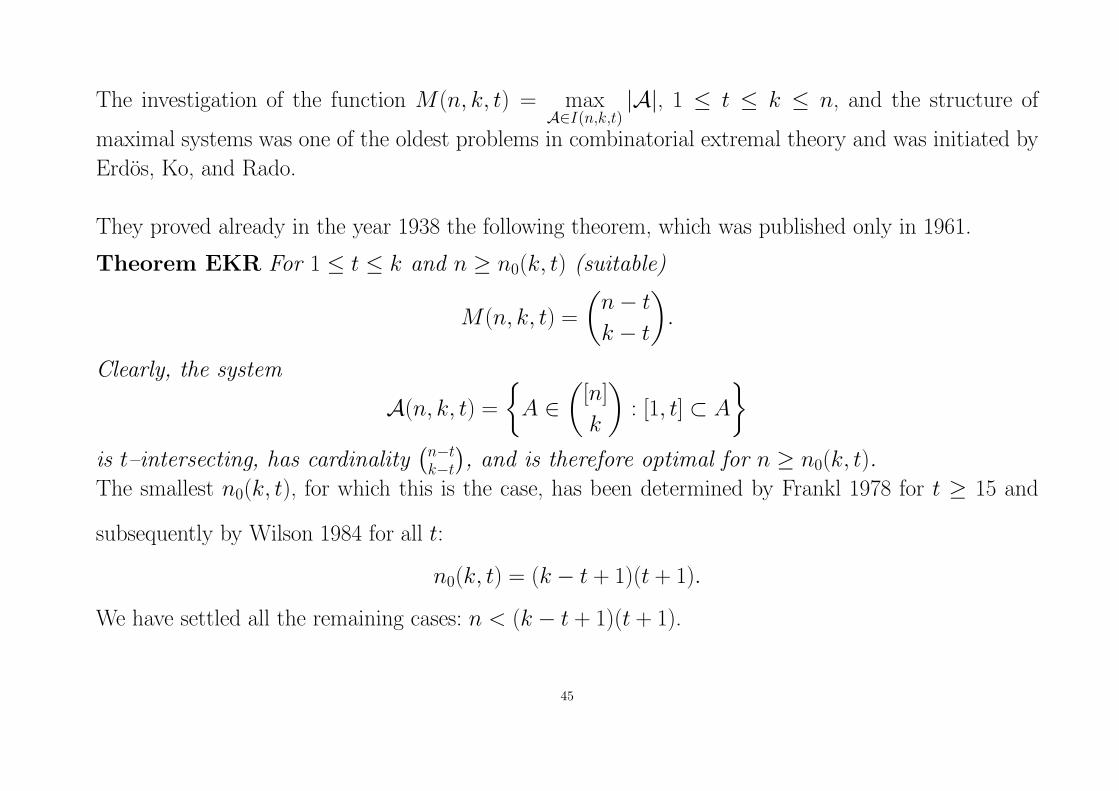
The investigation of the function M(n, k, t) = maxA∈I(n,k,t)

|A|, 1 ≤ t ≤ k ≤ n, and the structure of

maximal systems was one of the oldest problems in combinatorial extremal theory and was initiated by

Erdos, Ko, and Rado.

They proved already in the year 1938 the following theorem, which was published only in 1961.

Theorem EKR For 1 ≤ t ≤ k and n ≥ n0(k, t) (suitable)

M(n, k, t) =

(n − t

k − t

)

.

Clearly, the system

A(n, k, t) =

{

A ∈(

[n]

k

)

: [1, t] ⊂ A

}

is t–intersecting, has cardinality(n−t

k−t

), and is therefore optimal for n ≥ n0(k, t).

The smallest n0(k, t), for which this is the case, has been determined by Frankl 1978 for t ≥ 15 and

subsequently by Wilson 1984 for all t:

n0(k, t) = (k − t + 1)(t + 1).

We have settled all the remaining cases: n < (k − t + 1)(t + 1).

45

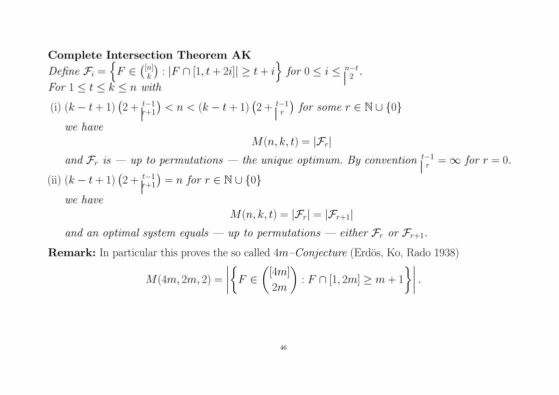
Complete Intersection Theorem AK

Define Fi ={

F ∈(

[n]k

): |F ∩ [1, t + 2i]| ≥ t + i

}

for 0 ≤ i ≤ n−t

2.

For 1 ≤ t ≤ k ≤ n with

(i) (k − t + 1)(2 + t−1

r+1

)< n < (k − t + 1)

(2 + t−1

r

)for some r ∈ N ∪ {0}

we have

M(n, k, t) = |Fr|and Fr is — up to permutations — the unique optimum. By convention t−1

r= ∞ for r = 0.

(ii) (k − t + 1)(2 + t−1

r+1

)= n for r ∈ N ∪ {0}

we have

M(n, k, t) = |Fr| = |Fr+1|and an optimal system equals — up to permutations — either Fr or Fr+1.

Remark: In particular this proves the so called 4m–Conjecture (Erdos, Ko, Rado 1938)

M(4m, 2m, 2) =

∣∣∣∣

{

F ∈(

[4m]

2m

)

: F ∩ [1, 2m] ≥ m + 1

}∣∣∣∣.

46

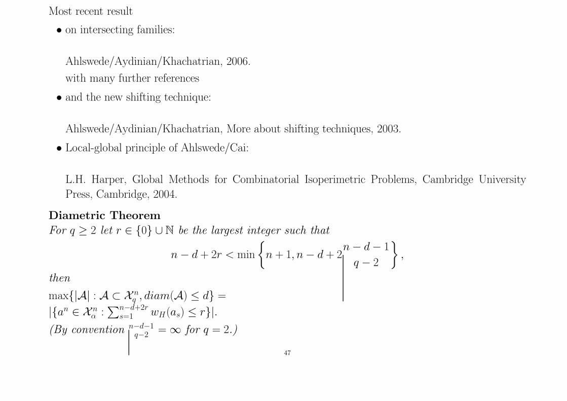
Most recent result

• on intersecting families:

Ahlswede/Aydinian/Khachatrian, 2006.

with many further references

• and the new shifting technique:

Ahlswede/Aydinian/Khachatrian, More about shifting techniques, 2003.

• Local-global principle of Ahlswede/Cai:

L.H. Harper, Global Methods for Combinatorial Isoperimetric Problems, Cambridge University

Press, Cambridge, 2004.

Diametric Theorem

For q ≥ 2 let r ∈ {0} ∪ N be the largest integer such that

n − d + 2r < min

{

n + 1, n − d + 2n − d − 1

q − 2

}

,

then

max{|A| : A ⊂ X nq , diam(A) ≤ d} =

|{an ∈ X nα :∑

n−d+2rs=1 wH(as) ≤ r}|.

(By convention n−d−1q−2

= ∞ for q = 2.)

47

Another diametric theorem in Hamming spaces: optimal group anticodes

R. Ahlswede

In the last century together with Levon Khachatrian we established a diametric theorem in Hamming

space Hn = (X n, dH).

Now we contribute a diametric theorem for such spaces, if they are endowed with the group structure

Gn =n∑

1G, the direct sum of group G on X = {0, 1, . . . , q− 1}, and as candidates are considered which

form a subgroup of Gn.

For all finite groups G, every permitted distance d, and all n ≥ d subgroups of Gn with

diameter d have maximal cardinality qd.

Other extremal problems can also be studied in this setting.

48

A report on Extremal Problems in Number Theory and especially also in Combinatorics,

which arose in Information Theory can be found in

R. Ahlswede, Advances on extremal problems in Number Theory and Combinatorics, European

Congress of Mathematicians, Barcelona 2000, Vol. I, 147.175, Progress in Mathematics, Vol. 201.

R. Ahlswede and V. Blinovsky, Modern Problems in Combinatorics, forthcoming book.

K. Engel, Sperner Theory, Cambridge University Press, Cambridge, 1997.

General Theory of Information Transfer and Combinatorics, Report on a Research Project at the

ZIF (Center of interdisciplinary studies) in Bielefeld Oct. 1, 2001 – August 31, 2004, edit R. Ahlswede

with the assistance of L. Baumer and N. Cai, Lecture Notes in Computer Science, No. 4123.

49

IX Network Coding for Information Flows

Combinatorial

Extremal

Problems Information

Networks

The founder of Information Theory Claude E. Shannon, who set the standards for efficient transmission

of channels with noise by introducing the idea of coding - at a time where another giant John

von Neumann was still fighting unreliability of systems by repetitions -

Shannon also wrote together with Peter Elias and Amiel Feinstein a basic paper on networks containing

the L.R. Ford/D.R. Fulkerson - Min Cut - Max Flow Theorem, saying that for flows of physical com-

modities like electric currents or water, satisfying Kirchhoff’s laws, the maximal flow equals the minimal

cut.

With the stormy development of Computer Science there is an ever increasing demand for designing

and optimizing Information Flows over networks - for instance in the Internet.

Data, that is strings of symbols, are to be send from sources s1, . . . , sn to their destinations, sets of node

sinks D1, . . . , Dn.50

Computer scientist quickly realized that it is beneficial to copy incoming strings at processors sitting

at nodes of the network and to forward copies to adjacent nodes. This task is called Multi-Casting.

However, quite surprisingly they did not consider coding, which means here to produce not only

copies, but, more generally, new output strings as deterministic functions of incoming strings.

The Min-Max-Theorem was discovered and proved for Information Flows by Ahlswede,

Cai, Li, and Yeung (2000).

Its statement can be simply explained. For one source only, that is n = 1, in the notation above, and

D1 = {d11, d12, . . . , d1t} let F1j denote the Max-Flow value, which can go for any commodity like water

in case of Ford/Fulkerson from si to d1i. The same water cannot go to several sinks. However, the amount

of min1≤j≤t F1j bits can go simultaneously to d11, d12, . . . and d1t. Obviously, this is best possible.

It has been referred to as ACLY-Min-Max-Theorem (It also could be called Shannon’s Missed

Theorem). To the individual F1j Ford/Fulkerson’s Min-Cut-Max-Flow Theorem applies.

It is very important that in the starting model there is no noise and it is amazing for how long Computer

Scientists did the inferior Multicasting allowing only copies.

Network Flows with more than one source are much harder to analyze and lead to a wealth of old

and new Combinatorial Extremal problems. This is one of the most striking examples of an

interplay between Information Transfer and Combinatorics.

51

Even nicely characterized classes of error correcting codes come up as being isomorphic to a

complete set of solutions of flow problems without errors!

Also our characterization of optimal Anticodes obtained with the late Levon Khachatrian arises in

such a role!

On the classical side for instance orthogonal Latin Squares - on which Euler went so wrong - arise.

The Min-Max-Theorem has been made practically more feasible by a polynomial algorithm by Peter

Sanders, Sebastian Egner and Ludo Tolhuizen as well as by his competitors (or groups of competitors)

in other parts of the world, leading to the joint publications.

With NetCod 2005 - the first workshop on Network Coding Theory and Applications, April 7, 2005,

Riva, Italy the New Subject Network Coding was put to start.

Research into network coding is growing fast, and Microsoft, IBM and other companies have research

teams who are researching this new field.

A few American universities (Princeton, MIT, Caltec and Berkeley) have also established research groups

in network coding.

The holy grail in network coding is to plan and organize ( in an automated fashion) network flow (that

is to allowed to utilize network coding) in a feasible manner. Most current research does not yet address

this difficult problem.

52

There may be a great challenge not only coming to Combinatorics but also to Algebraic Geome-

try and its present foundations.

An Introduction to the area of Network Coding is given in the book of R. Yeung.

The case |Di ∩ Dj| = ∅ for i 6= j and |Di| = 1 for i = 1, . . . , n, that is, each source sends its

message to its sink has an obvious symmetry and appeal. Soren Riis established the equivalence of

this flow problem to a guessing game, which is cooperative.

53

X. Localized Errors

A famous problem in coding theory consists in finding good bounds for the maximal size, say N(n, t, q),

of a t-error correcting code over a q-ary alphabet Q = {0, 1, . . . , q − 1} with blocklength n.

This code concept is suited for communication over a q-ary channel with input and output alphabets

Q, where a word of length n sent by the encoder is changed by the channel in atmost t letters. Here

neither the encoder nor the decoder knows in advance where the errors, that is changes of letters, occur.

It is convenient to use the notation relative error τ = t/n and rate R = n−1 log M .

The Hamming bound is an upper bound on it.

Hq(τ ) =

{

1 − hq(τ ) − τ logq(q − 1) if 0 ≤ τ ≤ q−1q

0 if q−1q

< τ ≤ 1.

We turn now to another model. Suppose that the encoder, who wants to encode message i ∈ M =

{1, 2, . . . , M}, knows the t-element set E ⊂ [n] = {1, . . . , n} of positions, in which only errors may

occur. He then can make the codeword presenting i dependent on E ∈ Et =(

[n]t

), the family of t-element

subsets of [n]. We call them “a priori error pattern”. A family {ui(E) : 1 ≤ i ≤ M, E ∈ Et} of q-ary

vectors with n components is an (M, n, t, q)l code (for localized errors), if for all E, E′ ∈ Et and all

q-ary vectors e ∈ V (E) = {e = (e1, . . . , en) : ej = 0 for j 6∈ E} and e′ ∈ V (E′)

ui(E) ⊕ e 6= ui′(E′) ⊕ e

′ for i 6= i′,

where ⊕ is the addition modulo q.

54

We denote the capacity error function, that is the supremum of the rates achievable for τ and all large n,

by C lq. It was determined by Bassalygo/Gelfand/Pinsker for the binary case to equal H2(τ ). For general

q the best known result is

Theorem Ahlswede/Bassalygo/Pinsker

(i) C lq(τ ) ≤ Hq(τ ), for 0 ≤ τ ≤ 1

2.

(ii) C lq(τ ) = Hq(τ ), for 0 ≤ τ <

12− q−2

2q(2q−3).

Competing Ideas:

Ahlswede: With increase of q the Hamming space should become more flexible for packing.

Pinsker: Knowing the a-priori error pattern E gives less (protocol) information if q increases.

Who wins?

55

XI. Search

After we wrote with I. Wegener one of the first books on search in 1978, the subject has grown terrifically.

Still progress is possible on basic questions

Input alphabet X = Q and output alphabet Y = Q.

Mf(n, t, q) maximal size of a t-error correcting code over a q-ary alphabet with block length n in the

presence of noiseless feedback, that means

Having sent letters x1, . . . , xj−1 ∈ X the encoder knows the letters y1, . . . , yj−1 ∈ Y received before he

sends the next letter xj (j = 1, 2, . . . , n).

Relative error τ = t/n and rate R = n−1 log M .

Cfq (τ ) the supremum of the rates achievable for τ and all large n (capacity error function).

56

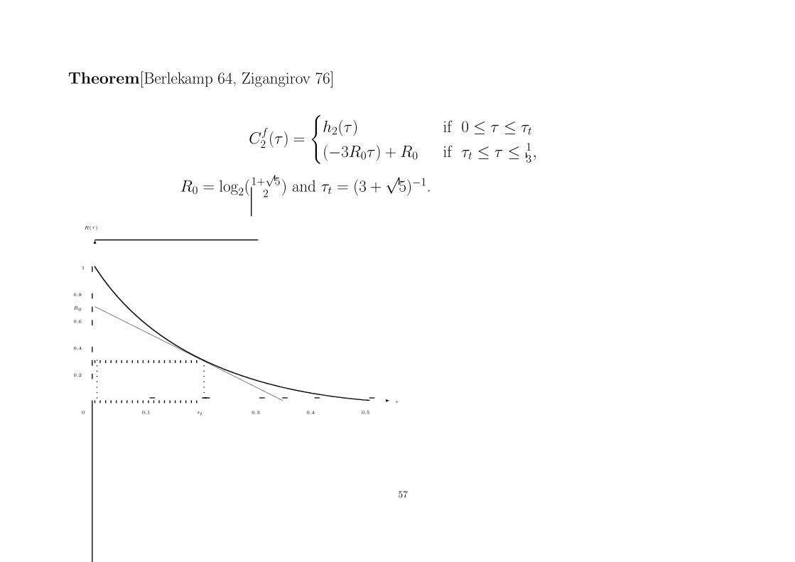
Theorem[Berlekamp 64, Zigangirov 76]

Cf

2 (τ ) =

{

h2(τ ) if 0 ≤ τ ≤ τt

(−3R0τ ) + R0 if τt ≤ τ ≤ 13,

R0 = log2(1+

√5

2 ) and τt = (3 +√

5)−1.

R(τ)

τ-

6

0 0.1 τt 0.3 0.4 0.5

0.2

0.4

0.6

R0

0.8

1

57

Theorem[Ahlswede, Deppe, Lebedev, Annals of the EAS, 2006]

Let q ≥ 3

(i)

Cf

q (τ )

≤ Hq(τ ) if 0 ≤ τ ≤ 1q

= (1 − 2τ ) logq(q − 1) if 1q≤ τ ≤ 1

2

= 0 if 12≤ τ ≤ 1

(ii) The rate function obtained by the r-rubber method is a tangent to Hq(τ ) going through ( 1r+1, 0).

τ-

6

0 0.1 0.2 0.3 0.4 0.5

0.2

0.4

0.6

0.8

1

58

The rubber method

b : M → {1, 2, . . . , q − 1}n−2t

bijection between messages and of used sequences.

The “0” is used for error correction only.

Given i ∈ M the sender chooses b(i) = (x1, x2, . . . , xn−2t) ∈ {1, 2, . . . , q − 1}n−2t as a skeleton for

encoding, which finally will be known to the receiver.

For all positions i ≤ n not needed dummy xi = 1 are defined to fill the block length n.

Transmission algorithm:

The sender sends x1, x2 until the first error occurs, say in position p with xp sent.

If a standard error occurs (xp → yp ∈ {1, 2, . . . , q − 1}), the sender transmits, with smallest l pos-

sible, 2l + 1 times 0 until the decoder received l + 1 zeros. Then he transmits at the next step xp, again,

and continues the algorithm.

If a towards zero error occurs (xp → yp = 0), the sender decreases p by one (if it is bigger than 1)

and continues (transmits at the next step xp).

Decoding algorithm: The receiver just regards the “0” as a a protocol symbol - he erases it by a

rubber, who in addition erases the previous symbol.

59

Example: n = 5, t = 2, q = 3

b(1) = 1, b(2) = 2

Let i = 1:

sent: 10111 10101 10001

received: 20111 20201 22001

r-rubber method:

skeleton: {xn−(r+1)t ∈ {0, 1, . . . , q − 1}n−(r+1)t : the sequence contains ≤ r − 1 consecutive zeros }protocol string: r consecutive zeros

60

Relation between Berlekamp’s strategies and r-rubber method

- For q = 2 and r > 1 the r-rubber strategies have the same rate as Berlekamp’s strategies (tangents to

the Hamming bound going through ( 1r+1

, 0)).

- Especially for q = 2 and r = 2 we get Berlekamp’s tangent bound.

- More general we get for q > 2 and r ≥ 1 tangents to the Hamming bound going through ( 1r+1

, 0).

61

Ratewise-optimal non-sequential search strategies under constraints on the tests

R. Ahlswede

Already in his Lectures on Search Renyi suggested to consider a search problem, where an unknown

x ∈ X = {1, 2, . . . , n} is to be found by asking for containment in a minimal number m(n, k) of subsets

A1, . . . , Am with the restrictions |Ai| ≤ k <n

2for i = 1, 2, . . . , m.

Katona gave in 1966 the lower bound m(n, k) ≥ log n

h(k

n)in terms of binary entropy and the upper bound

m(n, k) ≤⌈

log n+1log n/k

⌉

· n

k, which was improved by Wegener in 1979 to m(n, k) ≤

⌈log n

log n/k

⌉ (⌈n

k

⌉− 1).

We prove here for k = pn that m(n, k) = log n+o(log n)h(p) , that is, ratewise optimality of the entropy

bound.

Quite surprisingly, eventhough this result is known for several decades nobody proved

that – or even seems to have wondered whether – it is essentially best possible

for instance for k-set tests “carrying h(

k

n

)bit of information”.

62

However, when we looked for a proof we realized an obstacle, which blocked the development even for

people who may have believed in the entropy bound. The known proofs for upper bounds (Theorem KW

in Section 3) are constructive and apparently hard to improve. In such a situation often a probabilistic

argument helps. However, a standard approach by random choice is suboptimal even for the

simple case of unrestricted tests as was noticed already by Renyi 1965. Using the uniform distribution

for choosing a separating system (see Section 2) requires

m ≥ 2 log n + 6

sets, where ⌈log n⌉ is optimal. So we are by a factor of 2 away from the optimum!

63

XII. Combi-Probabilistic Models

Coloring Hypergraphs did a problem by Gallager

Slepian/Wolf Model 1973

for DMCS ((Xn, Y n))∞n=1.

-Y n Xn

Encoding f : Yn → N

Decoding g : X n × N → X n × Yn

Prob(g(Xn, f(Y n)) = (Xn

, Yn)) ∼ 1 (1)

Opt. Rate(f) = H(Y |X)

Gallager Model 1976

for discrete, memoryless conditional distribution

({Y n(xn) : xn ∈ X n})∞n=1 (Generic PY |X)

Prob(g(xn, f(Y n)) = (xn

, Yn)) ∼ 1 ∀x

n ∈ X n (2)

64

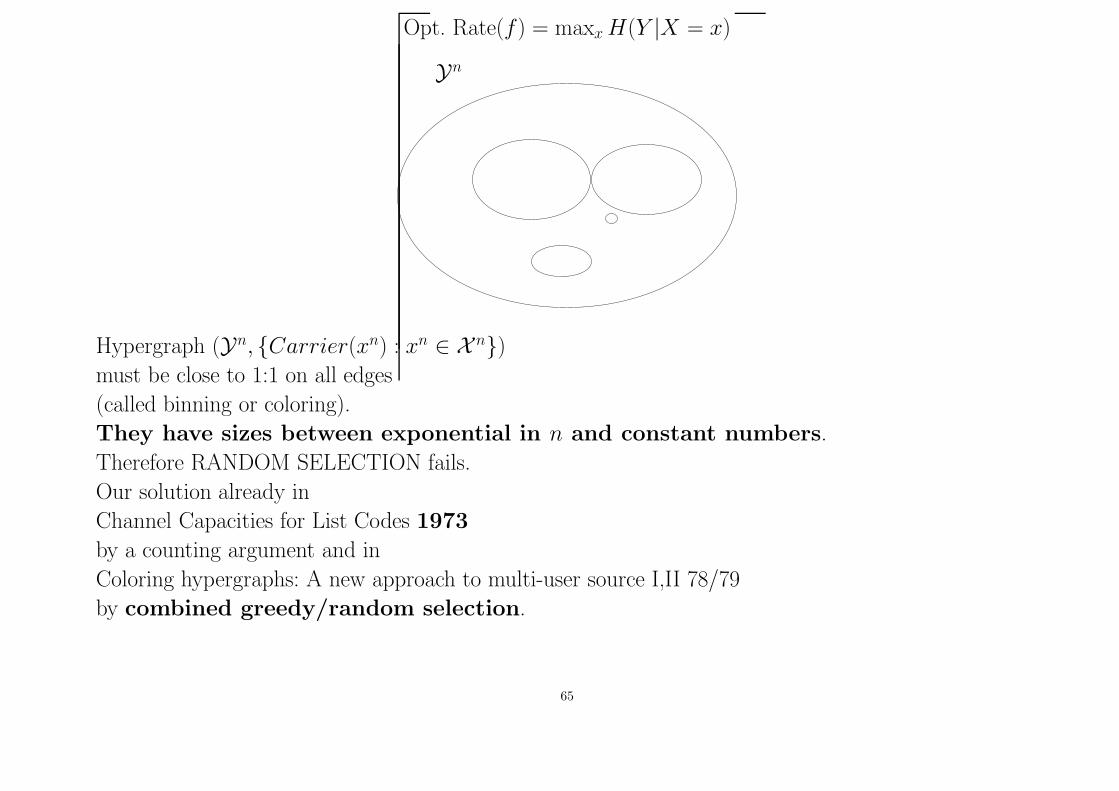
Opt. Rate(f) = maxx H(Y |X = x)

Yn

Hypergraph (Yn, {Carrier(xn) : xn ∈ X n})

must be close to 1:1 on all edges

(called binning or coloring).

They have sizes between exponential in n and constant numbers.

Therefore RANDOM SELECTION fails.

Our solution already in

Channel Capacities for List Codes 1973

by a counting argument and in

Coloring hypergraphs: A new approach to multi-user source I,II 78/79

by combined greedy/random selection.

65

C. Further Perspectives

a. Protocol Information (Gallager?)

“Protocol” information ought to be investigated more deeply. We encountered it in the Theory of

Localized Errors and in the Rubber Method.

66

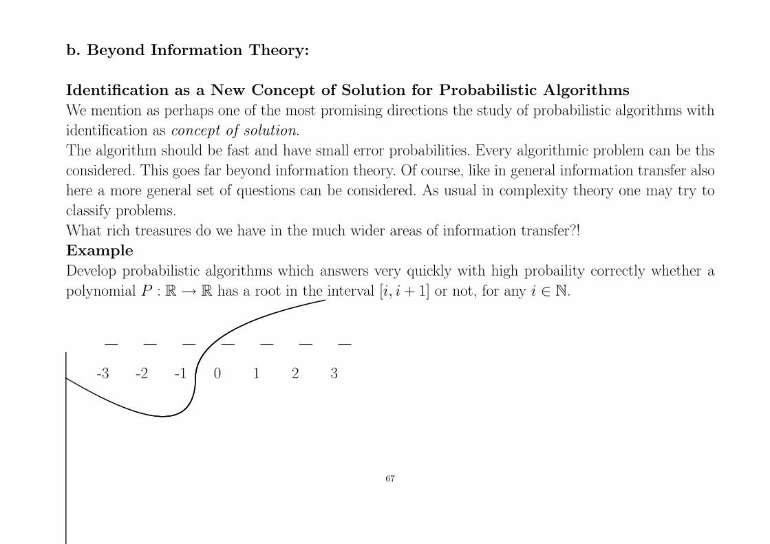
b. Beyond Information Theory:

Identification as a New Concept of Solution for Probabilistic Algorithms

We mention as perhaps one of the most promising directions the study of probabilistic algorithms with

identification as concept of solution.

The algorithm should be fast and have small error probabilities. Every algorithmic problem can be ths

considered. This goes far beyond information theory. Of course, like in general information transfer also

here a more general set of questions can be considered. As usual in complexity theory one may try to

classify problems.

What rich treasures do we have in the much wider areas of information transfer?!

Example

Develop probabilistic algorithms which answers very quickly with high probaility correctly whether a

polynomial P : R → R has a root in the interval [i, i + 1] or not, for any i ∈ N.

-3 -2 -1 0 1 2 3

67

c. A new connection between information inequalities

and Combinatorial Number Theory (Tao)

The final form of Tao’s inequality relating conditional expectation and conditional

mutual information

R. Ahlswede

Recently Terence Tao approached Szemeredi’s Regularity Lemma from the perspectives of Probability

Theory and of Information Theory instead of Graph Theory and found a stronger variant of this

lemma, which involves a new parameter.

To pass from an entropy formulation to an expectation formulation he found the following

Lemma. Let Y , and X, X ′ be discrete random variables taking values in Y and X , respectively, where

Y ⊂ [−1, 1], and with X ′ = f(X) for a (deterministic) function f .

Then we have

E(|E(Y |X ′) − E(Y |X)|

)≤ 2I(X ∧ Y |X ′)

1

2 .

We show that the constant 2 can be improved to (2ℓn2)1

2 and that this is the best possible constant.

68

d. A question to Shannon’s attorneys

The following last paragraph on page 376 is taken from “Two way commounication channels”, C.

Shannon Collected Papers, 351-384.

“The inner bound also has an interesting interpretation. If we artificially limit the codes to those where

the transmitted sequence at each terminal depends only on the message and not on the received sequences

at that terminal, then the inner bound is indeed the capacity region. This results since in this case we have

at each stage of the transmission (that is, given the index of the letter being transmitted) independence

between the two next transmitted letters. It follows that the total vector change in equivocation is

bounded by the sum of n vectors, each corresponding to an independent probability assignment. Details

of this proofs are left to the reader. The independence required would also occur if the

transmission and repetition points at each end were at different places with no direct

cross communication.”

According to my understanding the last sentence in this quote (which is put here in boldface) implies

the solution of the capacity region problem for what is now called Interference Channel. Already in

“A channel with two senders and two receivers”, 1974 I showed that the region obtained with

independent sender’s distributions is generally smaller than the capacity region.

69

e. Could we ask Shannon’s advise !!!

The following last paragraph on page 350 is taken from “Coding theorems for a discrete source with a

fidelity criterion”, C. Shannon Collected Papers, 325-350.

“In a somewhat dual way, evaluating the rate-distortion function R(D) for a source amounts, mathe-

matically, to minimizing a mutual Information under variant of the qi(j), again with a linear inequality

constraint. The solution leads to a function R(d) which is convex downward. Solving this problem cor-

responds to finding a channel that is just right for the source and allowed distortion level. This duality

can be pursued further and is related to the duality between past and future and the notions of control

and knowledge. Thus we may have knowledge of the past but cannot control it; we may

control the future but have no knowledge of it.”

The often cited last sentence, which we put here in boldface, has made several thinkers curious.

We sketch now our ideas about creating order involving knowledge of past and future and wonder

what Shannon would think about them. They are motivated by Clausius’ second law of

thermodynamics. He also introduced entropy.

70

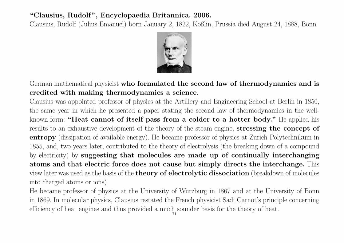
“Clausius, Rudolf”, Encyclopaedia Britannica. 2006.

Clausius, Rudolf (Julius Emanuel) born January 2, 1822, Koßlin, Prussia died August 24, 1888, Bonn

German mathematical physicist who formulated the second law of thermodynamics and is

credited with making thermodynamics a science.

Clausius was appointed professor of physics at the Artillery and Engineering School at Berlin in 1850,

the same year in which he presented a paper stating the second law of thermodynamics in the well-

known form: “Heat cannot of itself pass from a colder to a hotter body.” He applied his

results to an exhaustive development of the theory of the steam engine, stressing the concept of

entropy (dissipation of available energy). He became professor of physics at Zurich Polytechnikum in

1855, and, two years later, contributed to the theory of electrolysis (the breaking down of a compound

by electricity) by suggesting that molecules are made up of continually interchanging

atoms and that electric force does not cause but simply directs the interchange. This

view later was used as the basis of the theory of electrolytic dissociation (breakdown of molecules

into charged atoms or ions).

He became professor of physics at the University of Wurzburg in 1867 and at the University of Bonn

in 1869. In molecular physics, Clausius restated the French physicist Sadi Carnot’s principle concerning

efficiency of heat engines and thus provided a much sounder basis for the theory of heat.71

Entropy

Rudolf Clausius

∆S =∆Q

T

Einstein: Deepest law in physics

Boltzmann

−∑

pi log pi

(empirical distribution = composition = type = complexion)

Shannon

I(x ∧ y)

individual information

Identification Entropy

q

q − 1

(

1 −N∑

i=1

p2i

)

72

“The quantity∑

n

k=1 pk log21pk

is frequently called the entropy of the

distribution P = (p1, . . . , pk). Indeed, there is a strong connectionbetween the notion of entropy in thermodynamics and the no-tion of information (or uncertainly). L. Boltzmann was the firstto emphasize the probabilistic meaning of the thermodynamicalentropy and thus he may be considered as a pioneer of infor-mation theory. It would even be proper to call the formula theBoltzmann-Shannon formula. Boltzmann proved that the entro-py of a physical system can be considered as a measure of thedisorder in the system. In case of a physical system having manydegrees of freedom (e.g. perfect gas) the number measuring thedisorder of the system measures also the uncertainty concerningthe states of the individual particles.”

A. Renyi, Probability Theory, North Holland, Amsterdam, p. 554, 1970.

73

Creating order in sequence spaces

People spend a large amount of time creating order in various circumstances. Our aim is to start or

to contribute to a theory of ordering. In particular we try to understand how much “order” can be

created in a “system” under constraints on our “knowledge about the system” and on the “actions we

can perform in the system”.

The non-probabilistic model

We have a box that contains β objects at time t labeled with numbers from X = {1, . . . , α}. The state

of the box is st = (st(1), . . . , st(α)), where st(i) denotes the number of balls at time t labeled by i.

Assume now that an arbitrary sequence xn = (x1, . . . , xn) ∈ X n enters the box iteratively. At time t

an organizer O outputs an object yt and then xt enters the box. xn = (x1, . . . , xn) is called an input

and yn = (y1, . . . , yn) an output sequence. The organizer’s behaviour must obey the following rules.

74

Constraints on matter. The organizer can output only objects from the box. At each time t he

must output exactly one object.

Constraints on mind. The organizer’s strategy depends on

(a) his knowledge about the time t. The cases where O has a timer and has no timer are denoted by

T+ and T−, respectively.

(b) his knowledge about the content of the box. O− indicates that the organizer knows at time t only

the state st of the box. If he also knows the order of entrance times of the objects, we write O+.

(c) the passive memory (π, β, ϕ). At time t the organizer remembers the output letters yt−π, . . . , yt−1

and can see the incoming letters xt+1, . . . , xt+ϕ.

Let Fn(π, β, ϕ, T−, O−) be the set of all strategies for (T−, O−), length n and a given memory (π, β, ϕ)

and S be the set of all states. A strategy fn : X n ×S → X n assigns to each pair (xn, s1) an output yn.

Denote Y(fn) the image of X n × S under fn. Also denote ||Y(fn)|| the cardinality of Y(fn).

Now we define the size

Nn

α (π, β, ϕ) = min{||Y(fn)|| : fn ∈ Fn(π, β, ϕ, T−, O

−)}and the rate

να(π, β, ϕ) = limn→∞

1

nlog N

n

α (π, β, ϕ).

Analogously, we define in the case (T−, O+) the quantities Onα(π, β, ϕ), ωα(π, β, ϕ), in the case (T+, O−)

the quantities T nα (π, β, ϕ), τα(π, β, ϕ) and in the case (T+, O+) the quantities Gn

α(π, β, ϕ), γα(π, β, ϕ).

(d) the active memory. Now the organizer has additional memory of size m, where he is free to delete

or store any relevant information at any time. Here we are led to study the quantities Nnα (π, β, ϕ, m),

να(π, β, ϕ, m), etc.75

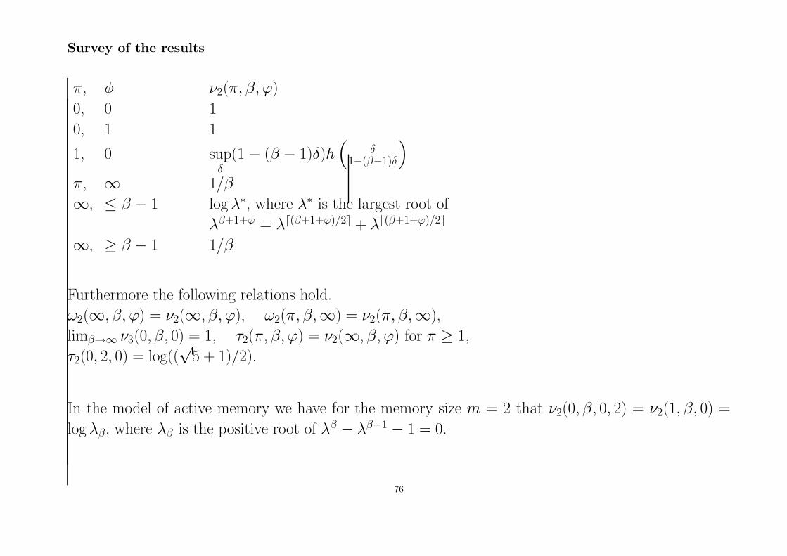
Survey of the results

π, φ ν2(π, β, ϕ)

0, 0 1

0, 1 1

1, 0 supδ

(1 − (β − 1)δ)h(

δ

1−(β−1)δ

)

π, ∞ 1/β

∞, ≤ β − 1 log λ∗, where λ∗ is the largest root of

λβ+1+ϕ = λ⌈(β+1+ϕ)/2⌉ + λ⌊(β+1+ϕ)/2⌋

∞, ≥ β − 1 1/β

Furthermore the following relations hold.

ω2(∞, β, ϕ) = ν2(∞, β, ϕ), ω2(π, β,∞) = ν2(π, β,∞),

limβ→∞ ν3(0, β, 0) = 1, τ2(π, β, ϕ) = ν2(∞, β, ϕ) for π ≥ 1,

τ2(0, 2, 0) = log((√

5 + 1)/2).

In the model of active memory we have for the memory size m = 2 that ν2(0, β, 0, 2) = ν2(1, β, 0) =

log λβ, where λβ is the positive root of λβ − λβ−1 − 1 = 0.

76

Conjecture 1. limϕ→∞ ν2(π, β, ϕ) 6= ν2(π, β,∞).

Conjecture 2. limβ→∞ να(0, β, 0) = log2⌈(α + 1)/2⌉(for α = 2 and α = 3 this is true).

Conjecture 3. ω2(0, β, 0) = ν2(1, β − 1, 0).

A probabilistic model

The initial content of the box and the input (Xt)nt=1 are produced by i.i.d. random variables with generic

distribution PX . This gives rise to an output process (Yt)nt=1. The constraints on matter and mind are

again meaningful. The performance of a strategy f is now measured by the entropy H(Y n) and the

mean entropy Hf = lim supn→∞(1/n)H(Y n) to be minimized.

Define

ηα(π, β, ϕ, PX) = limn→∞

minfn

1

nH(Y n).

For this model we obtained the following result. Consider the events Ek = {Y k = 01010 · · · } and

Dk = Ek r Ek+1. Denote q(k) =Prob(Dk).

Then for PX(0) = PX(1) = 1/2 we have

η2(∞, 2, 0, PX) =H(q)

∑∞k=1 kq(k)

.

77

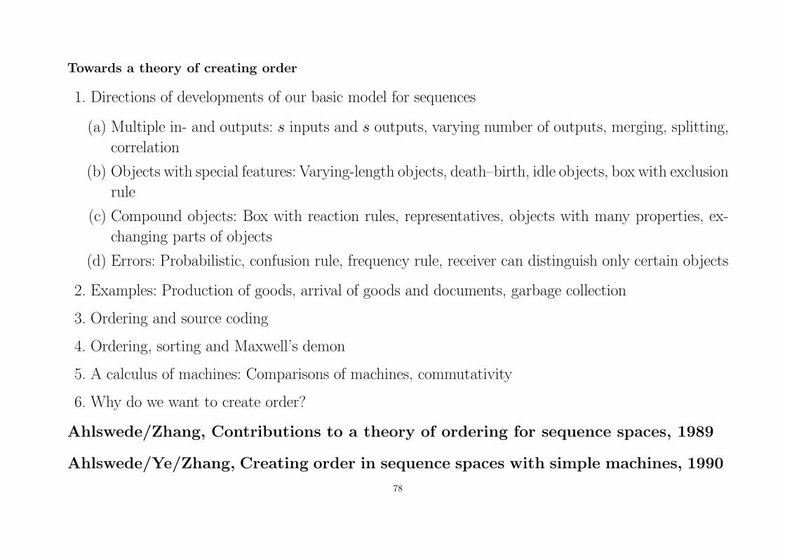
Towards a theory of creating order

1. Directions of developments of our basic model for sequences

(a) Multiple in- and outputs: s inputs and s outputs, varying number of outputs, merging, splitting,

correlation

(b) Objects with special features: Varying-length objects, death–birth, idle objects, box with exclusion

rule

(c) Compound objects: Box with reaction rules, representatives, objects with many properties, ex-

changing parts of objects

(d) Errors: Probabilistic, confusion rule, frequency rule, receiver can distinguish only certain objects

2. Examples: Production of goods, arrival of goods and documents, garbage collection

3. Ordering and source coding

4. Ordering, sorting and Maxwell’s demon

5. A calculus of machines: Comparisons of machines, commutativity

6. Why do we want to create order?

Ahlswede/Zhang, Contributions to a theory of ordering for sequence spaces, 1989

Ahlswede/Ye/Zhang, Creating order in sequence spaces with simple machines, 1990

78