1

Towards A Conceptually Simple DefensiveApproach for Few-shot classifiers Against

Adversarial Support SamplesYi Xiang Marcus Tan, Penny Chong, Jiamei Sun, Ngai-Man Cheung, Yuval Elovici and Alexander Binder

Abstract—Few-shot classifiers have been shown to exhibitpromising results in use cases where user-provided labels arescarce. These models are able to learn to predict novel classessimply by training on a non-overlapping set of classes. Thiscan be largely attributed to the differences in their mechanismsas compared to conventional deep networks. However, this alsooffers new opportunities for novel attackers to induce integrityattacks against such models, which are not present in othermachine learning setups. In this work, we aim to close this gapby studying a conceptually simple approach to defend few-shotclassifiers against adversarial attacks. More specifically, we pro-pose a simple attack-agnostic detection method, using the conceptof self-similarity and filtering, to flag out adversarial supportsets which destroy the understanding of a victim classifier for acertain class. Our extended evaluation on the miniImagenet (MI)and CUB datasets exhibit good attack detection performance,across three different few-shot classifiers and across differentattack strengths, beating baselines. Our observed results allowour approach to establishing itself as a strong detection methodfor support set poisoning attacks. We also show that our approachconstitutes a generalizable concept, as it can be paired with otherfiltering functions. Finally, we provide an analysis of our resultswhen we vary two components found in our detection approach.

Index Terms—adversarial machine learning, adversarial de-fence, adversarial detection, detection, few-shot, self-similarity,filtering

I. INTRODUCTION

AN open topic in machine learning is the transferabilityof a trained model to a new set of prediction categories

without retraining efforts, in particular when some classeshave very few samples. Few-shot learning algorithms havebeen proposed to address this. Prediction and training in few-shot approaches are based on the concept of an episode. Eachepisode (task) comprises several labelled training samples perclass (i.e. 1 or 5), denoted as the support set, and query samples

This research is supported by both ST Engineering Electronics and NationalResearch Foundation, Singapore, under its Corporate Laboratory @ UniversityScheme (Programme Title: STEE Infosec-SUTD Corporate Laboratory). (Cor-responding author: Yi Xiang Marcus Tan, e-mail:marcustanyx16@gmail.com).

Yi Xiang Marcus Tan, Penny Chong, Jiamei Sun was with the InformationSystems Technology and Design Pillar, Singapore University of Technologyand Design, Singapore 487372, Singapore.

Ngai-Man Cheung is with the Information Systems Technology and DesignPillar, Singapore University of Technology and Design, Singapore 487372,Singapore.

Yuval Elovici is with the Department of Software and Information SystemsEngineerng, Ben-Gurion University of the Negev, 653 Beer-Sheva, Israel.

Alexander Binder is with the Department of Informatics, Digital SignalProcessing and Image Analysis group of the University of Oslo, 0373 Oslo,Norway.

for episodic testing called the query set. Unlike conventionalmachine learning setups, the prediction in few-shot models isrelative to the support set classes of an episode [1], [2], [3],[4], [5]. The label categories drawn in each episode varies andtraining is performed by on these randomised sets of classes.This allows for the iteration over varying prediction tasks whenlearning model parameters. Effectively, this learns a class-agnostic similarity metric which allows for generalisation tonovel categories [6], [7], [8].

Unfortunately, the adversarial susceptibility of models underthe few-shot classification setting remains relatively unex-plored, albeit gaining traction [9], [10]. This is compared tomodels under the standard classification setting, where such aphenomenon had been widely explored [11], [12], [13], [14],[15], [16]. The relative nature of predictions in few-shot setupsallows going beyond crafting adversarial test samples.

The attacker could craft adversarial perturbations for all n-shot support samples of the attacked class and insert them intothe deployment phase of the model. The goal is to misclassifytest samples of the attacked class regardless of the samplesdrawn in the other classes. In this work, we consider theimpact on the few-shot accuracy of the attacked class, inthe presence of adversarial perturbations, even when differentsamples were drawn for the non-attacked classes. This is ahighly realistic scenario as the victim could unknowingly drawsuch adversarial support sets during the evaluation phase oncethey were inserted by the attacker. The use of adversarialsamples to attack other settings than the one trained for areknown as transferability attacks.

In order to mitigate the adverse effects of adversarial attacks,several methods were proposed in the past. Such approachesaim to do so through detection [17], [18], [19] or throughmodel robustness [20], [21], [22], [23]. Though these methodswork well for neural networks under the conventional classifi-cation setting, they will fail on few-shot classifiers due to thelimited data issue that few-shot learners excel at. Furthermore,these defences were not trained to transfer its pre-existingknowledge towards a novel distribution of class samples,contrary to few-shot classifiers. With the aforementioned draw-backs in mind, we propose a conceptually simple methodfor performing attack-agnostic detection of adversarial supportsamples in this setting. We exploit the concept of support andquery sets of few-shot classifiers to measure the similarityof samples within a support set after filtering, for exampleby autoencoders. We perform this by randomly splitting theoriginal support set randomly into auxiliary support and query

This work has been submitted to the IEEE for possible publication. Copyright may be transferred without notice, after which this version may no longer beaccessible.

arX

iv:2

110.

1235

7v1

[cs

.LG

] 2

4 O

ct 2

021

2

sets, followed by filtering the auxiliary support and predictingthe query. If the samples are not self-similar, then we will flagthe support set as adversarial. To this end, we describe thecontributions of this work as follows:

1) We propose a simple yet novel attack-agnostic detectionmechanism against adversarial support sets in the do-main of few-shot classification. This is based on self-similarity under randomised splitting of the supportset and filtering, and is the first, to the best of ourknowledge, for the detection of adversarial support setsin few-shot classifiers. In particular, we show that few-shot learning can be equipped with strong detectionapproaches for support set poisoning attacks.

2) We analyse the effectiveness of such a detection ap-proach, when using various filtering functions of dif-fering mechanisms. To provide a form of comparison,we adopted two simple baselines with one being an un-supervised approach while the other being a supervisedmethod.

3) We investigate the effects of a unique white-box adver-sary against few-shot frameworks, through the lens oftransferability attacks. Rather than crafting adversarialquery samples similar to standard machine learningsetups, we optimise adversarial supports sets, in a settingwhere all non-target classes are varying. Various attackstrengths were explored to analyse the trend in ourdetection performance.

4) We provide further analysis on the detection perfor-mance of our algorithm when using different differentfiltering functions and also different formulation variantsof the aforementioned self-similarity quantity. Our anal-ysis establishes our proposed approach of self-similarityand filtering as a generalisable concept.

This work extends our prior work in [24], where weintroduce here an additional model in our experiments, namelythe Prototypical Network (PN) [25], to improve the generalis-ability of our approach to other variants of few-shot models.Furthermore, we explored additional filtering functions andbaselines, to analyse variations in detection performance ofour approach and to provide a simple benchmark. Morespecifically, we describe our newly explored baselines, namelythe Out-of-Distribution Image Detection (ODIN) and IsolationForest (IF) approaches in Sections III-D1 and III-D2, whileintroducing the Total Variation Minimisation (TVM) and BitReduction (BitR) in Sections IV-E and IV-F as additionalfilters. We have also increased the scope of the attack strengthswe considered, to show the trends of our detection perfor-mance at various scenarios. Comparing to our previous workin [24], we have vastly expanded our experiment settings. InSection V-D, we show an extension of our transferability attackanalysis by introducing varying degrees of attack strength, forthe two attack variants that were explored in this work. Fur-thermore, we explain our motivation for using self-similarityhere, which was missing in our prior work [24]. In SectionV-E, we further extend our analysis to show the trends ofour detection performance. We evaluated across the variousattack strengths and attack approaches, filtering functions and

baselines, the few-shot models, and datasets.

II. RELATED WORKS

A. Few-shot classification

With the aim of mitigating the high demand for labelleddata for deep neural networks (DNNs), few-shot classificationrecognises novel categories with only a few labelled samplesper class for training. Notable methods include metric-basedclassifiers [6], [8], [26], [7] and optimisation-based classifiers[2], [5]. Optimisation-based classifiers learn the initialisationparameters that can quickly generalise to novel categoriesor train a meta-optimiser that adaptively updates the modelparameters for novel classes. Metric-based classifiers learn adistance metric that compares the representations of imagesand generates similarity scores for classification, which madesignificant progress recently.

B. Poisoning of Support Sets

There is limited literature examining the poisoning of sup-port sets in meta-learning. [9] proposed an attack routine,Meta-Attack, extending from the highly explored ProjectedGradient Descent (PGD) attack [14]. They assumed a scenariowhere the attacker is unable to obtain feedback from the classi-fication of the query set. Hence, the authors used the empiricalloss on the support set to generate adversarial support sampleswhich hope to induce misclassification behaviours to unseenquery sets.

C. Autoencoder-based and Feature Preserving-based De-fences

There are two recent prior works which utilise autoencodersas to formulate their defence approach. [19] performs thedetection of such attacks using Non-parametric Scan Statistics(NPSS), based on hidden node activations from an autoen-coder. This NPSS score measures how anomalous a subset of anode activation is, given an input sample. The authors computesuch activations from both clean and adversarial images, com-pares them and compute the NPSS score. [22] proposed usingan autoencoder to reconstruct input samples such that onlythe necessary signals remain for classification. Their trainingmethod is a two-step process, first performing unsupervisedtraining for reconstruction throughout the autoencoder, and thesecond, training only the decoder based on the classificationloss of the input with respect to the ground truth. However,under the few-shot setting, fine-tuning based on the classifi-cation loss should be avoided because we would require largeenough samples from each class for the fine-tuning step. [23]attempts to stabilise sensitive neurons which might be moreprone to the effects of adversarial perturbations, by enforcingsimilar behaviours of the sensitive neurons between cleanand adversarial inputs through Sensitive Neurons Stabilising(SNS). As such, SNS tries to preserve the features betweenthe reconstructed image and the original image for adversarialrobustness by training their defended model, regularised ona feature preserving loss term between clean and adversarialfeatures. The method in [23] requires adversarial samples

3

during the training process which potentially makes defendingagainst unseen attacks challenging, since they were unseenduring training. In light of this, we proposed a detectionapproach which does not make use of any adversarial samples.Though we employed the concept of feature preserving as oneof our various filtering functions (introduced later in SectionIV), our approach is still different from [23] as it does notsuffer from this limitation. Hence, in our work, we adoptedan approach which does not require labelled data to train ourautoencoder for reconstruction, which we will elaborate furtherin Section IV.

III. BACKGROUND

A. Few-shot classifiers Used

A majority of the few-shot classifiers are trained withepisodes sampled from the training set. Each episode consistsof a support set S = {xs, ys}K∗Ns=1 with N labelled samplesper K classes, and a query set Q = {xq}

Nq

q=1 with Nqunlabelled samples from the same K classes to be classified,denoted as a K-way N -shot task. The metric-based classifierslearn a distance metric that compares the features of supportsamples xs and query sample xq for classification. Duringinference, the episodes are sampled from the test set that hasno overlapping categories with the training set.

In this work, we explored three known metric-based few-shot classifiers, namely the RelationNet (RN) [6], the Proto-typical Network (PN) [1], and a state-of-the-art model, theCross-Attention Network (CAN) [8]. The support and querysamples are first encoded by a backbone CNN to get theimage features {f cs | c = 1, . . . ,K} and fq , respectively.The feature vectors f cs and fq ∈ Rdf ,hf ,wf , where df , hf ,and wf are the channel dimension, height, and width of theimage features. If N > 1, f cs will be the averaged feature ofthe support samples from class c. To measure the similaritybetween f cs and fq , the RN model concatenates fq and f csalong the channel dimension pairwise and uses a relationmodule to calculate the similarities. The CAN model adoptsa cross-attention module that generates attention weights forevery {f cs , fq} pair. The PN model computes the mean of thesupport samples after extracting their features, for each way ofthe episode. The attended image features are further classifiedwith cosine similarity in the spirit of dense classification [27].

B. Threat Model

We assume that the attacker wants to invalidate the few-shotclassifier’s notion of a targeted class, t, unlike conventionalmachine learning frameworks where one is optimising singletest samples to be misclassified. The attacker wants to findan adversarially perturbed set of support images, such thatmisclassification of most query samples from class t occurs,regardless of the class labels of the other samples. He then re-places the defender support set for class t with the adversarialsupport. We assume that the attacker has white-box access tothe few-shot model (i.e. weights, architecture, support set). Theadversarial support set would classify itself as self-similar, thatis, they classify among each other as being within the same

class, visually appear as class t, but classify true query imagesof class t as belonging to another class.

We now clarify our definition of x used in our attacks.The attacks are applied on a fixed support set candidate(xt1, . . . , x

tnshot

) for the target class. In every iteration of thegradient-based optimisation, we sample all classes randomlyexcept for the target class. Specifically, we sample the supportsets S−t and query sets Q−t of all the other classes randomly,and we randomly sample the query samples of the target Qt,illustrated in the equations below. They are redrawn in everyiteration of the optimisation following a uniform distribution.

C−t ∼ Uniform(C \ {t})S−t, Q−t ∼ Uniform(x|c ∈ C−t), Qt ∼ Uniform(x|c = t)

x = (xt1, . . . , xtnshot

),

h(x) = h([xt1, . . . , xtnshot

, S−t], [Qt, Q−t]),(1)

where C is the set of all classes, and C−t the random setof classes used in the episode together without class t (thecardinality of C−t is K− 1 given a K-way problem). Here, his a few-shot classifier that takes in a support set and a queryset to return class prediction scores for the query samples. Thelast line in (1) indicates that the few-shot classifier h takes ina support set made up of x and S−t and a query set made upof Qt and Q−t, which is a simplification to the expression,to relate to (3) and (4). The adversarial perturbations δ andthe underlying gradients are computed only for each of thesupport samples x of the target class.

C. Attack Algorithms Used

1) Projected Gradient Descent (PGD): The Projected Gra-dient Descent (PGD) attack [14] computes the sign of thegradient of the loss function with respect to the input data asadversarial perturbations. For an adversarial candidate xi atthe ith iteration:

x0 = xoriginal + Uniform([−ε, ε]d), (2)xi = Clipx,ε{xi−1 + η sign(∇xL(h(xi−1), c))}, (3)

where h(.) is the prediction logits for classifier h of someadversarial candidate xt, L is the loss used during training(i.e. cross-entropy with softmax for image classification), ∇xLrepresents the gradients of the loss calculated with respect toxt, η is the step size and ε is the adversarial strength whichlimits the adversarial candidate xi within an ε bounded `∞ball. Before the iterative perturbation step, the attacker ini-tialises the starting adversarial candidate as a point uniformlysampled around xoriginal, bounded by ε. This maximises theloss of the adversarial candidate with respect to the sourceclass c, which aims to cause a misclassification.

2) Carlini & Wagner L2 (CW-L2): The Carlini & WagnerL2 (CW-L2) attack [13] finds the smallest δ that successfullyfools a target model using the Adam optimiser. Among thevarious white-box attacks, this approach is known to be highlyeffective in obtaining successful adversarial samples whileachieving a low adversarial perturbation magnitude. However,contrary to the previous white-box attacks, the CW-L2 is

4

a specifically targeted attack as it involves computing thedifference in logits between the targeted prediction and thecurrent highest scoring logit (which is not t). Their attacksolves the following objective function:

minδ||δ||2 + const · L(x+ δ, κ),

s.t. L(x′, κ) = max(−κ,maxi 6=t

(h(x′)i)− h(x′)t).(4)

The first term penalises δ from being too large by minimisingthe L2 norm of δ while the second term enforces mispre-diction. The value const is a weighting factor that controlsthe trade-off between finding a low δ and having a successfulmisprediction. h(·)i refers to the logits of prediction index iand t refers to the target prediction. κ is the confidence valuethat influences the logits score differences between the targetprediction t and the next best prediction i.

D. Baseline Algorithms Used

In our work, we used two algorithms designed to detectout-of-distribution samples, namely Out-of-Distribution ImageDetection (ODIN) and Isolation Forest (IF), which can beexploited to detect adversarial samples..

1) Out-of-Distribution Image Detection (ODIN): TheODIN approach [28] is a two-step process, first involving apreprocessing step and with the second performing detectionbased on the maximum scaled softmax probability score fromthe classifier. Their approach claims that introducing a smallperturbation and using temperature-scaled softmax probabilityscores can make in- and out-of-distribution samples moredistinguishable. The scaled softmax probabilities are based onsome temperature parameter, T , such that:

softmaxi(x, T ) =exp(hi(x)/T )∑C−1j=0 exp(hj(x)/T )

, (5)

for i ∈ [0, C) where C is the total number of classes. h isour classifier function that returns the prediction scores of theinput sample. For the preprocessing of the inputs, they adopteda similar approach introduced by [16] to perform a smallperturbation to increase the scaled softmax score. However,they performed standard gradient descent to minimise the lossincurred (i.e. cross-entropy with softmax), instead of the stan-dard gradient ascent, commonly used in adversarial attacks.More specifically, the preprocessed input, x is computed asfollows:

x = x− εODIN · sign(∇x − log(softmaxy(x, T ))), (6)

where y is the hard label prediction of the classifier h. Afterwhich, x is passed as inputs to h, where the maximum scaledsoftmax probability score is computed. The input is flaggedas an outlier if this maximum if lower than a certain thresholdvalue, calibrated based on some desired True Positive Rate.The authors noted that good detection rates occur at tempera-ture values above 100 (i.e. T > 100), though any value of Tabove that range does not significantly improve the detectionfurther.

2) Isolation Forest (IF): The IF, analogous to RandomForest, uses a collection of isolation trees (binary trees) thatpartitions the data based on randomly selected features of ran-domly selected values (between the minimum and maximumvalue of the selected feature) [29]. The algorithm works underthe observation that clean data performs deeper traversalsfrom the root of the isolation trees to the leaves, in contrastto anomalous data points, since they are scarce (i.e. lyingfurther away in the feature space as compared to clean data).Consequently, anomalous data lies closer to the root nodes ofthe isolation trees. The anomalous score of a sample, x, beingfed to an isolation tree is given as such:

s(x,M) = 2−E(height(x))/c(M) (7)

where height(x) is the length of the path from the root tothe leaf for some input x, c(M) is the average number ofunsuccessful searches in a binary search tree given M numberof nodes. A score closer to 1 exhibit strong abnormality whilescores much smaller than 0.5 indicates otherwise.

IV. DETECTION METHODOLOGY

Our detection-based defence is based on three components:a sampling of auxiliary query and support sets, filtering theauxiliary support sets and measuring an adversarial score withrespect to the unfiltered auxiliary query set. Our motivationis derived from a high self similarity phenomenon underattacks (high classification accuracy of adversarial samples),which was absent under normal cases (see Table II). As such,should filtering be performed on the auxiliary support set,we postulate that the auxiliary query set will be less selfsimilar to its auxiliary supports. In order to showcase thegeneralisability of using self similarity and filtering to detectadversarial samples, we adopted several filtering functionswith highly different mechanisms. We denote a statistic eitheraveraged over all possible splits or for a randomly drawn splitof a support set into auxiliary sets with filtering of the auxiliarysupports as self-similarity.

A. Auxiliary Sets

Support and query sets in few-shot classifiers can be chosenfreely, which implies that any specific sample can be chosento be part of the support or the query. Assuming we have asupport set for class c, we randomly split it into its auxiliarysupport and query sets, where Sc might be clean or adversarial:

Scaux ∪Qcaux = Sc and Scaux ∩Qcaux = ∅,such that |Scaux| = nshot − 1 and |Qcaux| = 1. (8)

The few-shot learner is now faced with a randomly drawn(n − 1)-shot problem, evaluating on one query sample perway, with the option to average the n possible splits.

B. Detection of Adversarial Support Sets

Our detection mechanism flags a support set as adversarialwhen auxiliary support samples, after filtering, are highly dif-ferent from the auxiliary query samples, as shown in Figure 1.Given a support set of class c, Sc, we split it randomly into two

5

auxiliary sets Scaux and Qcaux. We filter Scaux using a functionr(·) and use the resultant samples as the new auxiliary supportset to evaluate Qcaux. Following which, we obtain the logits ofQcaux both before and after the filtering of the auxiliary support(i.e. using Scaux and r(Scaux) respectively) and compute the L1

norm difference between them. The adversarial score Uadv isgiven in (9) where h is the few-shot classifier

Uadv =‖h(r(Scaux), Qcaux)− h(Scaux, Qcaux)‖1, (9)

and r is any filtering function which maps a support setonto its own space. We observe that we obtain already veryhigh AUROC detection scores when computing Uadv withoutaveraging over nshot draws, which we elaborate further later.We flag a support set Sc as adversarial if the adversarial scoregoes above a certain threshold (i.e. Uadv > T ). Differentstatistics can be used to compute Uadv , with Eq. (9) beingone of many. Our main contribution lies rather in the proposalof using self-similarity of a support set for such detection.

Fig. 1: Illustration of our detection mechanism based on self-similarity, by partitioning Sc into two auxiliary sets Scaux andQcaux and filtering. Best viewed in colour.

C. Feature-space Preserving Autoencoder (FPA) for AuxiliarySupport Set Filtering

In light of exploring a DNN-based filtering function, weuse an autoencoder (AE) as function r(·) for the detectionof adversarial samples in the support set motivated by [22].We initially trained a standard autoencoder to reconstructthe clean samples in the image space using the MSE loss.However, the standard autoencoder performed poorly in de-tecting adversarial supports since it did not learn to preservethe feature space representation of image samples. Therefore,we switched to a feature-space preserving autoencoder whichadditionally reconstructs the images in the feature space ofthe few-shot classifier, contrary to prior work where they fine-tuned their AE on the classification loss [22]. We argue thatusing classification loss for fine-tuning is inapplicable in few-shot learning due to having very few labelled samples. Weminimise the following objective function for the feature-spacepreserving autoencoder:

LFPA =1

N ′

N ′∑i=1

0.01 · ‖xi − xi‖22

dim(xi)1/2+‖fi − fi‖22dim(fi)1/2

, (10)

where xi and xi are the original and reconstructed image sam-ples, respectively, and fi and fi are the feature representation

of the original and reconstructed image obtained from the few-shot model before any metric module (i.e. features from CNNbackbone). The second loss term ensures that the reconstructedimage features are similar to those of the original image in thefeature space of the few-shot models. We train the feature-space preserving autoencoder by fine-tuning the weights fromthe standard autoencoder.

D. Median Filtering (FeatS)

In our work, we also explored an alternate filtering function.We adopted a feature squeezing (FeatS) filter from [17],where it was used in a conventional classifier. It essentiallyperforms local spatial smoothing of images by having thecentre pixel taking the median value among its neighbourswithin a 2x2 sliding window. As their detection performancewas reasonably high using this filter, we decided to use it asan alternative to FPA as an explorative step. However, theirapproach performs filtering on each individual test samplewhereas we use it on the auxiliary support set.

E. Total Variation Minimisation (TVM)

We have also explored another filtering function, basedon the concept of TVM, in our work [30]. In essence, theTVM approach performs a reconstruction of randomly selectedpixels in the image, selected via a Bernoulli distribution. Thereconstruction involves solving an optimisation problem, byminimising the difference between the original and recon-structed images, regularised on the difference between thepixels to the left and above the selected pixel. We made useof the authors’ code, as implemented in [30], in our work.

F. Bit Reduction (BitR)

Other than FeatS, we have also adopted a bit reduction(BitR) filter similarly from [17]. It essentially reduces therange of values that each pixel in the image can take. Forinstance, reducing each pixel (pix) from an 8-bit precision(r = 8) to a 4-bit precision (r = 4) implies reducing therange of values from pix ∈ [0, 255] to pix ∈ [0, 15]. Note thatthis operation was also performed across all colour channels.

V. EXPERIMENTS AND RESULTS

A. Experimental Settings

1) Datasets: MiniImagenet (MI) [31] and CUB [32]datasets were used in our experiments. We prepared themfollowing prior benchmark splits [33], [34], with 64/16/20categories for the train/val/test sets of MI and 100/50/50categories for the train/val/test sets of CUB. In our attack anddetection evaluation, we chose an exemplary set of 10 and 25classes from the test set for MI and CUB respectively, andwe report the average metrics across them. This is purely forcomputational efficiency. For the RN model, we used imagesizes of 224 while using image sizes of 96 for the CAN andPN models across both datasets.

6

2) Attacks: In this work, we used two different attackroutines, one being PGD while the other being a slight variantof the CW-L2 attack. This variant uses a normal StochasticGradient Descent optimiser instead of Adam as we did notyield good performing adversarial samples with the latter. Westill used the objective function defined in (4) to optimiseour CW adversarial samples, while using (3) to perform aperturbation step less the clipping and sign functions. We namethis attack CW-SGD. For our PGD attack, we limit the L∞norm of the perturbation (ε∞) to 12/255 and a step size ofη = 0.05 (see (3)). For our CW-SGD attack, clipping wasnot used due to the optimisation over ||δ||2 while κ = 0.1 andη = 50. We have also evaluated the detection performances ona weaker variant of the above attacks (lower strength attacksettings). Namely, for PGD, we limit the L∞ norm of theperturbation to 6/255 and 3/255. For CW-SGD, we exploredthe settings κ = 0, η = 50 and κ = 0, η = 25. We would liketo stress that optimising for the best set of hyperparametersfor generating attacks is not the main focus of our work as weare more interested in obtaining viable adversarial samples. Inboth settings, we generate 50 sets of adversarial perturbationsfor each of the 10 and 25 exemplary classes for MI and CUBrespectively. We also attack all n support samples for thetargeted class t.

3) Autoencoder Training Hyperparameters: We used aResNet-50 [35] architecture for the autoencoders1. For the MIdataset, we trained the standard autoencoder from scratch witha learning rate of 1e-4. For the CUB dataset, we trained thestandard encoder initialised from ImageNet with a learningrate of 1e-4, and the standard decoder from scratch with alearning rate of 1e-3. For fine-tuning of the feature-spacepreserving autoencoder, we used a learning rate of 1e-4. Weemployed a decaying learning rate with a step size of 10epochs and γ = 0.1. We used the Adam [36] optimiser witha weight decay of 1e-4. In both settings, we used the trainsplit for training and the validation split for selecting our bestperforming set of autoencoder weights out of 150 epochs oftraining. It is implemented in PyTorch [37].

4) Training Few-shot Classifiers Hyperparameters: Wetrained the RN and CAN models on the MI and CUB datasets,following the details in [34] and [8]. The backbone CNNsfor RN and CAN models are Resnet-10 and Resnet-12 [35]respectively. The backbone for the PN model architecture wasa simple network with 4-convolutional blocks [25]. All modelsare trained under the 5-way 5-shot setting. For the CAN model,we trained with an SGD optimiser for 80 epochs with an initiallearning rate of 0.1. We annealed the learning rate to 0.06 atthe 60th epoch and 1e-3 at the 70th epoch. For the RN and PNmodels, we first pre-trained the backbone CNN on the trainingset as a standard classification task. With the pre-trained CNN,we further trained them with an Adam optimiser and a learningrate of 1e-3 for 400 epochs. We chose the best-performingmodel on the validation set for the following experiments.

1Autoencoder architecture adapted from GitHub repositoryhttps://github.com/Alvinhech/resnet-autoencoder.

B. Baseline Accuracy of Few-shot Classifiers

We evaluated our classifiers by taking the average andstandard deviation accuracy over 2000 episodes across allmodels and datasets, reported in Table I, to show that we wereattacking reasonably performing few-shot classifiers.

TABLE I: Baseline classification accuracy of the chosenmodels on the two datasets, under a 5-way 5-shot setting,computed across 2000 randomly sampled episodes. We reportthe mean with 95% confidence intervals for the accuracy.

RN - 5 shot CAN - 5 shot PN - 5 shotMI 0.727 ± 0.0037 0.787 ± 0.0033 0.662 ± 0.0038CUB 0.842 ± 0.0032 0.890 ± 0.0026 0.724 ± 0.0038

C. Evaluation Metrics Used

We evaluated the success of our attacks via computingthe Attack Success Rate (ASR), measuring the proportion ofsamples that had adversarial candidates generated from attacksthat successfully cause misclassification. We only consideredsamples originating from the targeted class when measuringASR:

ASR = ESt,Qt∼D{P (argmaxy(hy(St + δt, Qt)) 6= t)}.

(11)

The remaining (K − 1) classes were sampled randomly tomake up the support set.

In evaluation of the detection performances, we used theArea Under the Receiver Operating Characteristic (AUROC)metric, since detection problems are binary (whether an ad-versarial sample is present or not), and true and false positivescan be collected at various predefined threshold values.

D. Transferability Attack Results

TABLE II: Classification accuracy of the auxiliary query setunder various scenarios. “Clean” indicates that only cleansamples are present in the support set while “PGD” and“CW-SGD” indicates that the respective adversarial samplesare present in the support set. In the presence of adversarialsamples, both the auxiliary support and query set containsadversarial samples. We computed the results across the 10and 25 exemplary classes for MI and CUB respectively, and50 sets of adversarial perturbations.

Model Dataset Clean PGD(ε∞ = 12/255)

CW-SGD(κ = 0.1)

RN(5-shot)

MI 0.697 0.736 0.815CUB 0.834 0.947 0.919

CAN(5-shot)

MI 0.783 1.000 1.000CUB 0.876 0.999 0.987

PN(5-shot)

MI 0.679 0.999 0.993CUB 0.843 0.998 0.981

To begin with, the adversarial samples classify each other ata comparable or even better accuracy than clean samples do,and thus cannot be distinguished by looking at accuracy alone.We show the accuracy of the auxiliary query set when onlyclean support set is present and also when only adversarialsupport set is present in Table II. For the latter, it implies that

7

(a) Vanilla attack settings (i.e. ε∞ = 12/255 for PGD, κ = 0.1 andη = 50 for CW-SGD).

(b) Lower attack settings variant 1 (i.e. ε∞ = 6/255 forPGD, κ = 0 and η = 50 for CW-SGD).

(c) Lower attack settings variant 2 (i.e. ε∞ = 3/255 for PGD, κ = 0and η = 25 for CW-SGD).

Fig. 2: Transferability attack results under scenarios (i) Fixed Supports and (ii) New Supports, against our two explored attackson RN, PN and CAN models across both datasets. Reported ASRs were averaged across the chosen exemplary classes andacross the 50 generated sets of adversarial perturbations as bar charts. Standard deviation is represented as the whiskers. ASRmetric reported. Attack strength is sorted in the following order: (Figure 2a) > (Figure 2b) > (Figure 2c).

the adversarial samples are found both in the auxiliary supportand query sets. Our results illustrate the self-similar nature ofour adversarial support samples, which is not observed for theclean samples.

We conducted transferability experiments to evaluate howwell the attacker generalised their generated adversarial per-turbation under two unique scenarios: i) transfer with fixedsupports and ii) transfer with new supports. Setting (i) assumesthat we have the same adversarial support set for class tand we evaluated the ASR over newly drawn query sets.Setting (ii) relaxes this assumption and we instead appliedthe generated adversarial perturbation, that was stored duringthe attack phase, on newly drawn support sets for class t,

similarly evaluating over newly drawn query sets. Contrary totransferability attacks in conventional setups where a sampleis generated on one model and evaluated on another, weperformed transferability to new tasks, by drawing randomlysets of non-target classes together with their support sets, andnew query sets for the few-shot paradigm.

As illustrated in Figure 2, the PGD generated adversarialsamples showed higher transferability than the CW-SGD at-tack, across the three models and under all scenarios. Theexceptionally high transfer ASR we observed under scenario(i) implies that once the attacker had obtained an adversarialsupport set targeting a specific class, successful attacks can becarried out on new tasks for which the target class is present.

8

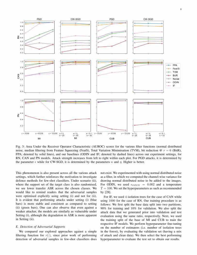
Fig. 3: Area Under the Receiver Operator Characteristic (AUROC) scores for the various filter functions (normal distributednoise, median filtering from Feature Squeezing (FeatS), Total Variation Minimisation (TVM), bit reduction @ r = 6 (BitR),FPA; denoted by solid lines), and our baselines (ODIN and IF; denoted by dashed lines) across our experiment settings, forRN, CAN and PN models. Attack strength increases from left to right within each plot. For PGD attacks, it is determined bythe parameter ε while for CW-SGD, it is determined by the parameters κ and η. Higher is better.

This phenomenon is also present across all the various attacksettings, which further reinforces the motivation to investigatedefence methods for few-shot classifiers. Under scenario (ii),where the support set of the target class is also randomised,we see lower transfer ASR across the chosen classes. Wewould like to remind readers that the adversarial sampleswere optimised explicitly using setting (i) and not for (ii).It is evident that performing attacks under setting (i) (bluebars) is more stable and consistent as compared to setting(ii) (green bars). One can also observe that even against aweaker attacker, the models are similarly as vulnerable underSetting (i), although the degradation in ASR is more apparentin Setting (ii).

E. Detection of Adversarial SupportsWe compared our explored approaches against a simple

filtering function for r(·), since prior work of performingdetection of adversarial samples in few-shot classifiers does

not exist. We experimented with using normal distributed noiseas a filter, in which we computed the channel-wise variance fordrawing normal distributed noise to be added to the images.For ODIN, we used εODIN = 0.002 and a temperatureT = 100. We set the hyperparameters as such as recommendedby [28].

For IF, we used 4 isolation trees for the case of CAN whileusing 1000 for the case of RN. Our training procedure is asfollows: We first split the base data split into two partitions,90% for training and 10% for validation. We also split theattack data that we generated prior into validation and testevaluation using the same ratio, respectively. Next, we usedthe training split of the base of MI and CUB to train therespective IF models. We perform hyperparameter fine-tuningon the number of estimators (i.e. number of isolation treesin the forest), by evaluating the validation set (having a mixof attack and clean data). We then select the best performinghyperparameter to evaluate the test set to obtain our results.

9

Our results in Figure 3 shows that FPA exhibits gooddetection performance across all settings. Though “FeatS”also exhibit good detection performances, the FPA approachconsistently outperforms it across all settings for RN andCAN, regardless of the attack strength (denoted by the solidblue line chart). The “Noise” approach (denoted by the solidred line chart), however, encountered challenges in detectionand is arguably the worse performing among the other filteringfunctions and outlier detection approaches, when observingthe trends for RN and CAN. We see highly varied detectionperformances across the different settings, which makes thisapproach highly unreliable. This result is hardly surprisingsince such methods require substantial manual fine-tuning ofits noise parameters. This is not ideal as newer attacks canbe introduced in the future and also, being in a few-shotframework, the optimal noise parameters between differenttask instances might not be consistent as the data mightbe different. However, the FPA filter approach exhibits suchrobustness even in such scenarios as it still achieved favourableAUROC scores. For clean samples, the FPA managed toreconstruct Scaux such that the logits of Qcaux before andafter filtering remained consistent, even when the FPA didnot encounter classes from the novel split during training.Although our outlier baselines (i.e. ODIN and IF; denotedby the dashed line charts) perform well at times, they canfail at other settings, which also makes them less reliable inperforming detection. This phenomenon can also be seen forthe BitR filter function, where it performs reasonably well forthe CAN model but not for the RN and for the PN models.We note that for BitR, better detection performances couldbe observed when the detection threshold was flipped (i.e.Uadv > T to Uadv < T ). Therefore, we flipped the detectioncondition for BitR for all models.

VI. DISCUSSION

A. Detection Performance of Attacking Single Sample inCrafting Adversarial Support Sets

We have also explored the effectiveness of our attack detec-tion algorithm when the attacker only attacks a single samplein the support set. We only considered the CAN model in thisset of experiments as the behaviour for the case of RN willbe similar. We evaluated the AUROC scores when using ourFPA filtering function, with Figure 4 illustrating our results.We chose this setting as we wanted to shed some light on theimpact of our detection approach, should we adopt anothersetting (i.e. attacking N samples vs attacking 1 sample).Attackers adopting a scenario between these two settingswould yield results which will simply be an interpolation ofthe two.

It is clear that the detection AUROC score suffers as lessadversarial samples were found in our support set. This ishardly surprising as there might be instances whereby theadversarial sample was found in the auxiliary query set, ren-dering the filtering function useless in filtering the adversarialsample. However, even when faced with a single adversarialsample, our algorithm could still detect adversarial supportsto a reasonable extent. One could also take the average

Fig. 4: AUROC results comparing between attacking 1 sampleand 5 samples in the support set for the CAN, using our FPAto filter the auxiliary support set. We computed the resultsacross the 10 and 25 exemplary classes for MI and CUBrespectively, and 50 sets of adversarial perturbations. Attackstrengths for PGD and CW-SGD were ε∞ = 12/255 andκ = 0.1 respectively.

of multiple random splits of auxiliary support and querysets instead to compute the adversarial score for performingdetection to improve the robustness of our detection approach.Furthermore, attacking a few-shot classifier with only a singlesample would not yield favourable attack outcomes as evidentin Figure 5, where we observe a transferability attack ASRdegradation as compared to attacking 5 samples. As such, anydetrimental impact attacker inflicts will be lessened as well.

Fig. 5: Transferability attack results under settings (i) FixedSupports and (ii) New Supports, against our two exploredattacks on the CAN model across both datasets, comparingbetween 1 sample and 5 samples being attacked in the adver-sarial support set. Reported ASRs were averaged across thechosen exemplary classes and across the 50 generated sets ofadversarial perturbations. Attack strengths for PGD and CW-SGD were ε∞ = 12/255 and κ = 0.1 respectively. ASRmetric reported.

B. Study of Self-Similarity Computation Methods

In Section IV-B, we described one of the possible detectionmechanism based on logits differences. An alternative wouldbe to use hard label predictions. Thus, we investigate the effectof different schemes as a justification for our choice Uadv . Forthe case of hard label predictions, we perform the following:we compute the average accuracy of Qcaux, across the different

10

permutated partitions of Sc. We illustrate how we constructour partitions across the n-shots in Figure 6. In essence, eachsupport sample will have a chance to be part of the auxiliaryquery set. This results in the statistic U ′adv:

Fig. 6: Illustration of how partitioning Sc into two auxiliarysets Scaux and Qcaux is performed. Best viewed in colour.

U ′adv =1

nshot

nshot∑i=1

1[argmaxj(hj(r(Sci,aux), Q

ci,aux)) 6= c],

(12)where h is the few-shot classifier, and r is the filteringfunction. Similarly, we flag the support set as adversarial whenU ′adv > T , such that it goes above a certain threshold.

TABLE III: Area Under the Receiver Operator Characteristic(AUROC) scores for the two detection mechanisms (Uadv andU ′adv) using our FPA across our experiment settings. Higheris better.

Model DatasetPGD

(ε∞ = 12/255)CW-SGD(κ = 0.1)

Uadv U ′adv Uadv U ′

advRN

(5-shot)MI 0.999 0.451 0.979 0.723

CUB 0.997 0.326 0.974 0.524CAN

(5-shot)MI 0.999 0.991 0.999 0.931

CUB 0.999 0.998 0.988 0.821PN

(5-shot)MI 0.999 0.903 0.973 0.558

CUB 0.999 0.997 0.942 0.782

TABLE IV: Area Under the Receiver Operator Characteristic(AUROC) scores for the two detection mechanisms (Uadv andU ′adv) using FeatS across our experiment settings. Higher isbetter.

Model DatasetPGD

(ε∞ = 12/255)CW-SGD(κ = 0.1)

Uadv U ′adv Uadv U ′

advRN

(5-shot)MI 0.998 0.585 0.936 0.714

CUB 0.983 0.275 0.899 0.551CAN

(5-shot)MI 0.995 0.304 0.963 0.008

CUB 0.985 0.154 0.986 0.768PN

(5-shot)MI 0.998 0.000 0.945 0.001

CUB 0.997 0.000 0.929 0.004

Tables III to VII show our AUROC scores comparing thetwo detection mechanisms, Uadv and U ′adv . It is evident thatusing logits scores to calculate differences, as in Uadv , is moreinformative than using hard label predictions to match classlabels, as Uadv outperforms U ′adv . Differences in logits canbe pronounced also in cases when the prediction label does

TABLE V: Area Under the Receiver Operator Characteristic(AUROC) scores for the two detection mechanisms (Uadv andU ′adv) using BitR across our experiment settings. Higher isbetter.

Model DatasetPGD

(ε∞ = 12/255)CW-SGD(κ = 0.1)

Uadv U ′adv Uadv U ′

advRN

(5-shot)MI 0.415 0.002 0.297 0.006

CUB 0.518 0.004 0.444 0.001CAN

(5-shot)MI 0.938 0.000 0.999 0.002

CUB 0.939 0.000 0.972 0.013PN

(5-shot)MI 0.357 0.286 0.422 0.240

CUB 0.057 0.153 0.261 0.114

TABLE VI: Area Under the Receiver Operator Characteristic(AUROC) scores for the two detection mechanisms (Uadv andU ′adv) using Noise across our experiment settings. Higher isbetter.

Model DatasetPGD

(ε∞ = 12/255)CW-SGD(κ = 0.1)

Uadv U ′adv Uadv U ′

advRN

(5-shot)MI 0.765 0.460 0.455 0.562

CUB 0.779 0.200 0.605 0.525CAN

(5-shot)MI 0.657 0.137 0.007 0.000

CUB 0.868 0.437 0.024 0.004PN

(5-shot)MI 0.998 0.551 0.902 0.558

CUB 0.997 0.697 0.885 0.554

not switch. We would like to note that when using U ′adv , forFeatS, BitR, and Noise filters, there is a greater majority ofAUROC scores that fall below 0.5. This indicates that betterperformance would be achieved when the flagging conditionis inverted. However, it will not be experimentally consistentsince such inversion should be applied on both Uadv and U ′adv ,for any given filter function.

C. Varying Degrees of Regularisation of FPA

We observe lower AUROC scores for the RN model than theCAN model in Figure 3. As such, we question if this differencecan be attributed to the FPA’s ability to reconstruct clean sam-ples effectively, as mentioned in the preamble of Section IV.Recalling from (10), we define an additional regularisationterm to enforce stricter reconstruction requirements to alsoinclude class distribution reconstruction. More specifically, weminimise the following objective function:

TABLE VII: Area Under the Receiver Operator Characteristic(AUROC) scores for the two detection mechanisms (Uadv andU ′adv) using TVM across our experiment settings. Higher isbetter.

Model DatasetPGD

(ε∞ = 12/255)CW-SGD(κ = 0.1)

Uadv U ′adv Uadv U ′

advRN

(5-shot)MI 0.813 0.891 0.520 0.764

CUB 0.756 0.813 0.559 0.802CAN

(5-shot)MI 0.938 0.814 0.983 0.861

CUB 0.968 0.819 0.948 0.860PN

(5-shot)MI 0.999 0.799 0.960 0.737

CUB 0.999 0.891 0.928 0.772

11

LFPA′ =1

N ′

N ′∑i=1

0.01· ‖xi − xi‖22

dim(xi)1/2+‖fi − fi‖22dim(fi)1/2

+‖zi − zi‖22dim(zi)1/2

,

(13)

where xi and xi are the original and reconstructed image sam-ples, respectively, and, fi and fi are the feature representationof the original and reconstructed image obtained from the few-shot model before any metric module, and zi and zi are thelogits of the original and reconstructed image. We refer to thisvariant as FPA′. Similarly, we train FPA′ by fine-tuning theweights from the standard autoencoder.

TABLE VIII: AUROC results comparing FPA and FPA′

for the RN. We computed the results across the 10 and 25exemplary classes for MI and CUB respectively, and 50 setsof adversarial perturbations.

DatasetPGD

(ε∞ = 12/255)CW-SGD(κ = 0.1)

FPA FPA′ FPA FPA′

MI 0.999 0.999 0.979 0.950CUB 0.997 0.997 0.974 0.971

Our results in Table VIII shows that surprisingly, imposing ahigher degree of regularisation marginally lowers the detectionperformance of our algorithm rather than improving it. Thisimplies that FPA is already sufficient to induce a large enoughdivergence in classification behaviours in the presence of anadversarial support set.

VII. CONCLUSION

In this work, we made several extensions from our priorwork. Firstly, we provide motivation to our conceptuallysimple approach by analysing the self-similarity of supportsamples under attack and normal conditions. Secondly, weperform a more in-depth analysis of our detection performanceagainst a wider range of attack strengths and also with an ad-ditional few-shot classifier. Thirdly, we provide an analysis ofthe transferability attack and our detection performance whenonly a single sample in the support set is targeted. Finally, westudy the effects of varying the self-similarity computationmethod on the detection performance. Through our extendedresults, we have shown that the FPA approach is still the mosteffective filtering function (highest AUROC scores) among theexplored filter functions, while also being able to outperformsimple baseline approaches across our settings. Our algorithm,which uses the concept of self-similarity among samples inthe support set and filtering, is thus shown to exhibit somegeneralizability in essence. Finally, in our single sample attackscenario, we found that although the detection performancedrops slightly, the transferability attack results decayed moresignificantly, which also provides a lower bound of our attackdetection performance in essence.

REFERENCES

[1] J. Snell, K. Swersky, and R. S. Zemel, “Prototypical networks for few-shot learning,” arXiv preprint arXiv:1703.05175, 2017.

[2] C. Finn, P. Abbeel, and S. Levine, “Model-agnostic meta-learning forfast adaptation of deep networks,” in Proceedings of the 34th ICMLVolume 70. JMLR. org, 2017, pp. 1126–1135.

[3] N. Mishra, M. Rohaninejad, X. Chen, and P. Abbeel, “A simple neuralattentive meta-learner,” in ICLR, 2018.

[4] A. Nichol and J. Schulman, “Reptile: a scalable metalearning algorithm,”arXiv preprint arXiv:1803.02999, vol. 2, no. 3, p. 4, 2018.

[5] Q. Sun, Y. Liu, T.-S. Chua, and B. Schiele, “Meta-transfer learning forfew-shot learning,” in Proceedings of the IEEE CVPR, 2019, pp. 403–412.

[6] F. Sung, Y. Yang, L. Zhang, T. Xiang, P. H. Torr, and T. M. Hospedales,“Learning to compare: Relation network for few-shot learning,” inProceedings of the IEEE CVPR, 2018, pp. 1199–1208.

[7] C. Zhang, Y. Cai, G. Lin, and C. Shen, “Deepemd: Few-shot imageclassification with differentiable earth mover’s distance and structuredclassifiers,” in IEEE/CVF CVPR, 2020, pp. 12 203–12 213.

[8] R. Hou, H. Chang, M. Bingpeng, S. Shan, and X. Chen, “Cross attentionnetwork for few-shot classification,” in NIPS, 2019, pp. 4005–4016.

[9] H. Xu, Y. Li, X. Liu, H. Liu, and J. Tang, “Yet meta learning can adaptfast, it can also break easily,” 2020.

[10] M. Goldblum, L. Fowl, and T. Goldstein, “Adversarially robust few-shotlearning: A meta-learning approach,” Advances in Neural InformationProcessing Systems, vol. 33, 2020.

[11] C. Szegedy, W. Zaremba, I. Sutskever, J. Bruna, D. Erhan, I. Goodfellow,and R. Fergus, “Intriguing properties of neural networks,” arXiv preprintarXiv:1312.6199, 2013.

[12] N. Papernot, P. McDaniel, I. Goodfellow, S. Jha, Z. B. Celik, andA. Swami, “Practical black-box attacks against machine learning,” inProceedings of the 2017 ACM on Asia Conference on Computer andCommunications Security, ser. ASIA CCS ’17. ACM, 2017, pp. 506–519. [Online]. Available: http://doi.acm.org/10.1145/3052973.3053009

[13] N. Carlini and D. Wagner, “Towards evaluating the robustness of neuralnetworks,” in 2017 IEEE Symposium on Security and Privacy (SP).IEEE, 2017, pp. 39–57.

[14] A. Madry, A. Makelov, L. Schmidt, D. Tsipras, and A. Vladu, “Towardsdeep learning models resistant to adversarial attacks,” in InternationalConference on Learning Representations, 2018.

[15] T. Tanay and L. Griffin, “A boundary tilting persepective on thephenomenon of adversarial examples,” arXiv preprint arXiv:1608.07690,2016.

[16] I. J. Goodfellow, J. Shlens, and C. Szegedy, “Explaining andHarnessing Adversarial Examples,” pp. 1–11, 2014. [Online]. Available:http://arxiv.org/abs/1412.6572

[17] W. Xu, D. Evans, and Y. Qi, “Feature squeezing: Detecting adversarialexamples in deep neural networks,” arXiv preprint arXiv:1704.01155,2017.

[18] S. Tian, G. Yang, and Y. Cai, “Detecting Adversarial Examples throughImage Transformation,” Aaai, pp. 4139–4146, 2018.

[19] C. Cintas, S. Speakman, V. Akinwande, W. Ogallo, K. Weldemariam,S. Sridharan, and E. McFowland, “Detecting adversarial attacks viasubset scanning of autoencoder activations and reconstruction error,”in IJCAI, 2020.

[20] H. Zhang, Y. Yu, J. Jiao, E. P. Xing, L. E. Ghaoui, and M. I. Jordan,“Theoretically principled trade-off between robustness and accuracy,”arXiv preprint arXiv:1901.08573, 2019.

[21] A. Jeddi, M. J. Shafiee, M. Karg, C. Scharfenberger, and A. Wong,“Learn2perturb: an end-to-end feature perturbation learning to improveadversarial robustness,” in Proceedings of the IEEE/CVF Conference onComputer Vision and Pattern Recognition, 2020, pp. 1241–1250.

[22] J. Folz, S. Palacio, J. Hees, and A. Dengel, “Adversarial defense basedon structure-to-signal autoencoders,” in 2020 IEEE Winter Conferenceon Applications of Computer Vision (WACV). IEEE, 2020, pp. 3568–3577.

[23] C. Zhang, A. Liu, X. Liu, Y. Xu, H. Yu, Y. Ma, and T. Li, “Interpretingand improving adversarial robustness of deep neural networks withneuron sensitivity,” IEEE Transactions on Image Processing, vol. 30,pp. 1291–1304, 2020.

[24] Y. X. M. Tan, P. Chong, J. Sun, N.-M. Cheung, Y. Elovici, and A. Binder,“Detection of adversarial supports in few-shot classifiers using self-similarity and filtering,” 2021.

[25] J. Snell, K. Swersky, and R. Zemel, “Prototypical networks for few-shotlearning,” in NIPS, 2017, pp. 4077–4087.

[26] M. Lichtenstein, P. Sattigeri, R. Feris, R. Giryes, and L. Karlinsky,“Tafssl: Task-adaptive feature sub-space learning for few-shot classifica-tion,” in Computer Vision – ECCV 2020, A. Vedaldi, H. Bischof, T. Brox,and J.-M. Frahm, Eds. Cham: Springer International Publishing, 2020,pp. 522–539.

12

[27] Y. Lifchitz, Y. Avrithis, S. Picard, and A. Bursuc, “Dense classificationand implanting for few-shot learning,” in Proceedings of the IEEEConference on Computer Vision and Pattern Recognition, 2019, pp.9258–9267.

[28] S. Liang, Y. Li, and R. Srikant, “Enhancing the reliability of out-of-distribution image detection in neural networks,” in InternationalConference on Learning Representations, 2018.

[29] F. T. Liu, K. M. Ting, and Z.-H. Zhou, “Isolation-based anomalydetection,” ACM Transactions on Knowledge Discovery from Data(TKDD), vol. 6, no. 1, pp. 1–39, 2012.

[30] C. Guo, M. Rana, M. Cisse, and L. van der Maaten, “Countering adver-sarial images using input transformations,” in International Conferenceon Learning Representations, 2018.

[31] O. Vinyals, C. Blundell, T. Lillicrap, D. Wierstra et al., “Matchingnetworks for one shot learning,” in NIPS, 2016, pp. 3630–3638.

[32] C. Wah, S. Branson, P. Welinder, P. Perona, and S. Belongie, “Thecaltech-ucsd birds-200-2011 dataset,” 2011.

[33] S. Ravi and H. Larochelle, “Optimization as a model for few-shotlearning,” in ICLR, 2017.

[34] H.-Y. Tseng, H.-Y. Lee, J.-B. Huang, and M.-H. Yang, “Cross-domainfew-shot classification via learned feature-wise transformation,” in ICLR,2020.

[35] K. He, X. Zhang, S. Ren, and J. Sun, “Deep residual learning for imagerecognition,” in Proceedings of the IEEE conference on computer visionand pattern recognition, 2016, pp. 770–778.

[36] D. P. Kingma and J. Ba, “Adam: A method for stochastic optimization,”arXiv preprint arXiv:1412.6980, 2014.

[37] A. Paszke, S. Gross, S. Chintala, G. Chanan, E. Yang, Z. DeVito, Z. Lin,A. Desmaison, L. Antiga, and A. Lerer, “Automatic differentiation inpytorch,” in NIPS-W, 2017.

Yi Xiang Marcus Tan graduated with a Ph.D. degree from the SingaporeUniversity of Technology and Design (SUTD) in 2021, where he was underthe supervision of Alexander Binder and Ngai-Man Cheung during hiscandidature. His research interest lies in the area of machine learning andhow machine learning can be defended against integrity attacks.

Penny Chong graduated with a Ph.D. degree from the Singapore University ofTechnology and Design (SUTD), under the supervision of Alexander Binderand Ngai-Man Cheung. She received a B.Sc. (Hons) in Applied Mathematicswith Computing from Universiti Tunku Abdul Rahman (UTAR), Malaysia in2016. Her research interests include machine learning, explainable AI and itsapplications.

Jiamei Sun graduated with a Ph.D. degree from the Singapore Universityof Technology and Design in 2021, where she was under the supervisionof Alexander Binder during her candidature. Her research interests includemachine learning, deep learning and explainable AI.

Ngai-Man Cheung is an associate professor at the Singapore Universityof Technology and Design. He received his Ph.D. degree in ElectricalEngineering from University of Southern California (USC), Los Angeles, CA,in 2008. His research interests include image, video and signal processing,computer vision and AI.

Yuval Elovici is the director of the Telekom Innovation Laboratories at Ben-Gurion University of the Negev (BGU), head of BGU Cyber Security ResearchCenter and a professor in the Department of Software and InformationSystems Engineering at BGU. He holds a Ph.D. in Information Systems fromTel-Aviv University. His primary research interests are computer and networksecurity, cyber security, web intelligence, information warfare, social networkanalysis, and machine learning. He is the co-founder of the start-up Morphisec.

Alexander Binder is an associate professor at the University of Oslo (UiO).He received a Dr.rer.nat. in Computer Science from Technische UniversitatBerlin in 2013. His research interests include explainable deep learning andmedical imaging.