Toward Constant time Enumeration by

Amortized Analysis

Toward Constant time Enumeration by

Amortized Analysis

27/Aug/2015 Lorentz Workshop for Enumeration Algorithms Using Structures

Takeaki Uno (National Institute of Informatics, Japan)

http://research.nii.ac.jp/~uno/index-j.htmle-mail: uno@nii.ac.jp

Approach from ComputationApproach from Computation

• I would like to start from PHILOSOPHY

• Personally, I think algo. researches are divided into three

+ Mathematical approaches

BP, approx., on-line, embedding, interior point method, sampling…

+ Structural approaches

　 graph class, miner, perfect graph conjecture, Voronoi diagram,…

+ Computation approaches

DP, branch&bound, k-best, plane sweep, prefix array,…

• Many in former, and less in latter (I don’t know it is good or not)

Computation Approach for Enumeration

Computation Approach for Enumeration

• In enumeration algorithms, many researches seem to follow computation approaches and structural approaches

• There are still many unstudied problems, so there would be a big frontier

• Today, I would like to talk about amortized analysis on enumeration algorithm that is in a computation approach

• So the talk is combination of complexity analysis, algorithm design, and structures

Complexity AnalysisComplexity Analysis

• Complexity analysis a base notion of algorithm design

• With complexity analysis we can design efficient algorithms

+ k-best selection

　　 reduce problems to 12/13 iteratively with tricky pivots

+ merge sort

balance of problem partition reduces time complexity

• We can not understand why the time complexity is small, without understanding the complexity analysis

Targets in This TalkTargets in This Talk

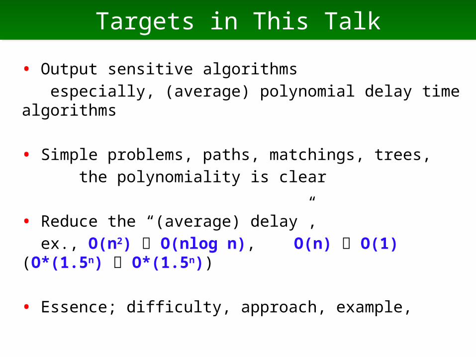
• Output sensitive algorithms

especially, (average) polynomial delay time algorithms

• Simple problems, paths, matchings, trees,

the polynomiality is clear

• Reduce the “(average) delay”,

ex., O(n2) O(nlog n), O(n) O(1) (O*(1.5n) O*(1.5n))

• Essence; difficulty, approach, example,

2 Motivation to Amortization2 Motivation to Amortization

There is an AlgorithmThere is an Algorithm

• Suppose that there is an enumeration algorithm Z.

we want to know time complexity of Z (output polynomiality)

• What is needed?

• What will we obtain as a result?

• We assume that Z is a tree-shaped recursion algorithm

(the structure of the recursion is a tree)

and the problem is combinatorial.

(has at most 2n solutions)

・・・・・・

Iteration = O(X)Iteration = O(X)

• We now know that each iteration takes O(X) time.

Can we do something?

No. Possibility for

“exponentially many iterations, with few solutions”

ex) feasible solutions for SAT,

with branch-and-bound algorithm

・・・・・・

O(X)

O(X)

Solution for EachSolution for Each

• We now know that each iteration outputs a solution.

Can we do something?

Yes! #solutions = #iterations

“O(X) time for each solution”

・・・・・・

O(X)

O(X)

Solutions at LeavesSolutions at Leaves

• We now know that at each leaf, a solution is output.

Can we do something?

ex) s-t paths, spanning trees, …

No. Possibility for

“exponentially many inner

iterations, with few leaves”

・・・・・・

O(X)

O(X)EXP. many

Bounded DepthBounded Depth

• We now know that the height of recursion tree is at most H

Can we do something?

YES! [#iterations] < [#solutions] × [height]

“O(X ・ H) time for each solution”

・・・・・・

O(X)

O(X) O(H)

At least Two ChildrenAt least Two Children

• Instead of the height, we now know that each non-leaf iteration

has at least two children

Can we do something?

YES! [#iterations] < 2 × [#solutions]

“O(X) time for each solution”

・・・・・・

O(X)two

two two

Good Three CasesGood Three Cases

• These three cases are typical in which we can bound the time complexity efficiently

• In each case, the time complexity for an iteration depends on maximum computation time on an iteration

• If we want to do better,

we have to use amortized analysis

(average computation time of

an iteration) ・・・・・・

two

two two

・・・・・・

・・・・・・

3 Basic Analysis3 Basic Analysis

Bottom-widenessBottom-wideness

• An iteration of enumeration algorithm generates recursive calls for solving “subproblems”

• Subproblems are usually smaller than the original problem

Many bottom level iterations take short time, few iterations take long time (we call bottom-wideness)

• Can we do something better?

・・・・・・

longmiddle

short shortshortshort

middle

Bad CaseBad Case

• An iteration of enumeration algorithm generates recursive calls for solving “subproblems”

• Subproblems are usually smaller than the original problem

Many bottom level iterations take short time, few iterations take long time

• Can we do something better?

No. not sufficient

in the right case, an iteration

takes O(n) time on average 1

1

1

1

1

nn-1

n-2

2・

・・

・・

・

BalancedBalanced

• The recursion tree was biased. If balanced?

No. not sufficient

in the right case, an iteration

takes O(n) time on average

nn-1 n-1

n-2 n-2

1 1 1 1 1

What is sufficient to reduce the amortized time complexity?

Sudden DecreaseSudden Decrease

• In the cases, sudden decrease occurs.

time for parent and child differ much

We shall clarify good

characterization for

“no sudden decrease”

• Then, what is good?n

n-1 n-1n-2 n-2

1 1 1 1 1

1

1

1

1

1

nn-1

n-2

2

・・

・・

・・

Toy CaseToy Case

• If any iteration has two children, and the computation time decreases constantly, the amortized computation time will be reduced

Ex)

n + 2(n-1) + 4(n-2) +…+ 2n-1•2 + 2n•1

2•2n

• This holds for any polynomial

{Σ 2n-i poly(i) } / 2•2n = O(1)

・・・・・・

nn-1 n-1

n-2 n-2

1 1 1 1 1

computation time

#iterations

= O(1)

AnalysisAnalysis

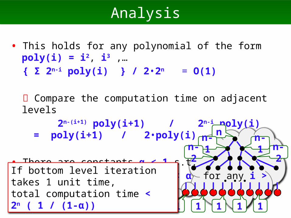
• This holds for any polynomial of the form poly(i) = i2, i3 ,…

{ Σ 2n-i poly(i) } / 2•2n = O(1)

Compare the computation time on adjacent levels

2n-(i+1) poly(i+1) / 2n-i poly(i) = poly(i+1) / 2•poly(i)

• There are constants α < 1 s.t.

poly( i+1) / 2•poly( i ) < α for any i > 0

・・・・・・

nn-1 n-1

n-2 n-2

1 1 1 1 1

If bottom level iteration takes 1 unit time,total computation time < 2n ( 1 / (1-α))

Generalization of the Toy CaseGeneralization of the Toy Case

• Assume that poly(i) is an arbitrary polynomial

• There are constant δ and α < 1 s.t.

poly(i+1) / 2•poly( i ) < α for any i > δ

• When i < δ, poly(i) is constant, thus any iteration on level

below δ takes constant time

• For i ≥ δ ,

{ Σi ≥δ 2n-i poly(i) } / 2•2n(n-δ) = O(1)

・・・・・・

nn-1 n-1

n-2 n-2

1 1 1 1 1

Therefore, amortized computation time for one iteration is O(1)

More Than Two ChildrenMore Than Two Children

• Consider cases that an iteration may generate more than two recursive calls (so, iterations have three or more children)

• Let N(i) be the number of iterations in level i

computation time on level i is bounded by Σ N(i) poly(i)

• Compare adjacent levels

N(i+1) poly(i+1) / N(i) poly(i)

≤ poly(i+1) / 2•poly(i)

・・・・・・

nn-1

n-2

1 1 1 1 1

・・・・・・Thus, in the same way, we can show amortized computation time for one iteration is O(1)

ApplicationApplication

• You may think this is too much trivial to enumeration algorithms

• However, surprisingly, there are applications

• Consider the enumeration of

elimination orderings

Elimination ordering

for given a structure (graph, set, etc.)

a way of removing its elements one by one until the structure will be empty, with keeping a given property

・・・・・・

nn-1 n-1

n-2 n-2

1 1 1 1 1

Elimination Ordering for ConnectivityElimination Ordering for Connectivity

Ex) For given a connected graph G=(V,E), remove vertices one by one with keeping the connectivity

• We can enumerate this elimination

ordering by simple backtracking

• Each iteration takes O(|V|2) time

Iter (G, S) 1. if G is empty then output S 2. for each vertex v in G, if G-v is connected then call Iter (G-v, S+v)

…unpublished

Necessary ConditionNecessary Condition

(1) For any connected graph, there are at least two vertices whose removals are connected

Each (internal) iteration has at least two children

(2) Computation time on an iteration in level i is O(i2)

Amortized computation time of

and iteration is O(1) time

Iter (G, X)1. if G is empty then output X2. for each vertex v in G if G-v is connected then call Iter (G-v, X+v)

Small Pit FallsSmall Pit Falls

How to output X in O(1) time?

output X by the difference from the previously output one

Since the number of additions and deletions is linear in the number of iterations, the amortized output time is O(1)

How to give G and X to the recursive call in O(1) time?

always update them, and give them by pointers to G and X

Before the recursive call, we remove v and adjacent edges from G, and add v to X

After the recursive call, we add v and adjacent edges to G, and

remove v from X. This doesn’t increase the time/space complexity

Q

Q

Other Elimination OrderingOther Elimination Ordering

• There are many kinds of elimination orderings

+ perfect elimination ordering (chordal graphs)

+ strongly perfect elimination ordering (chordal graphs)

+ vertex on the surface of the convex hull (points)

…

+ edge coloring of bipartite graph can be also solved

• At least, there proposed constant time algorithms for the first two

(technical, to achieve amortized constant time for each iteration)

• We can have the same results with very very simple algorithms

Ruskey et. al. ‘03

Ruskey et. al. ‘03

Matsui & U ‘05

4 Amortize by Children4 Amortize by Children

Biased Recursion TreesBiased Recursion Trees

• The previous cases are something perfect

+ the height (depth) is equal at everywhere

+ computation time depends on the height

• We want to have stronger tools

that can be applied to biased cases

・・・・・・

nn-1 n/2

n-2 n/4

1 1 1 1 1

Well-known CaseWell-known Case

• Let T(X) be the computation time on iteration X

• If every child takes at most T(X) / α, for some α > 1

the height of the tree is O(log n)

+ useful in complexity analysis

+ however, #iterations is bounded by

polynomial (not fit for enumeration)

・・・・・・

nn/3 n/2

n/6 n/4

1 1 1 1 1

We need another idea

Local AmortizationLocal Amortization

• If #children is large, amortized time complexity will be small even though sudden decrease occurs

• Let C(X) be children of iteration X,

and assign computation time T(X) to its children

each child receives T(X) / |C(X)|

• The time complexity of an iteration is

O( max X { T(X) / ( |C(X)| + 1) } )

• We can use #grandchildren instead of #children

10

2

22

2 2 2 2

Estimating #(Grand)ChildrenEstimating #(Grand)Children

• This analysis needs to estimate #children (and #grandchildren)

this will be a technical part of the proof

+ estimate by the degree of the pivot vertex

+ #edges in a cycle

+ #edges in a cut…

・・・

Enumeration of s?-pathEnumeration of s?-path

Problem: given a graph G=(V,E), and a vertex s, enumerate all simple paths one of whose end is s

• Simply, by back tracking, we can solve

• Each iteration takes O(d(t)) where d(t) is the degree of t

the time complexity of an iteration is O(|V|)

Iter (G=(V,E), t, S)1. output S2. for each vertex v in G adjacent to s call Iter (G-t, v, S+v)

ss

…folklore

AmortizationAmortization

+ Each iteration takes O(d(t)) time

+ Each iteration generates d(t) recursive calls

• Thus, max x { T(X) / ( |C(X)| + 1) } = O(1),

and the amortized time complexity of

an iteration is O(1)

Iter (G=(V,E), s, S)1. output S2. for each vertex v in G adjacent to s call Iter (G-s, v, S+v)

ss

Other ProblemsOther Problems

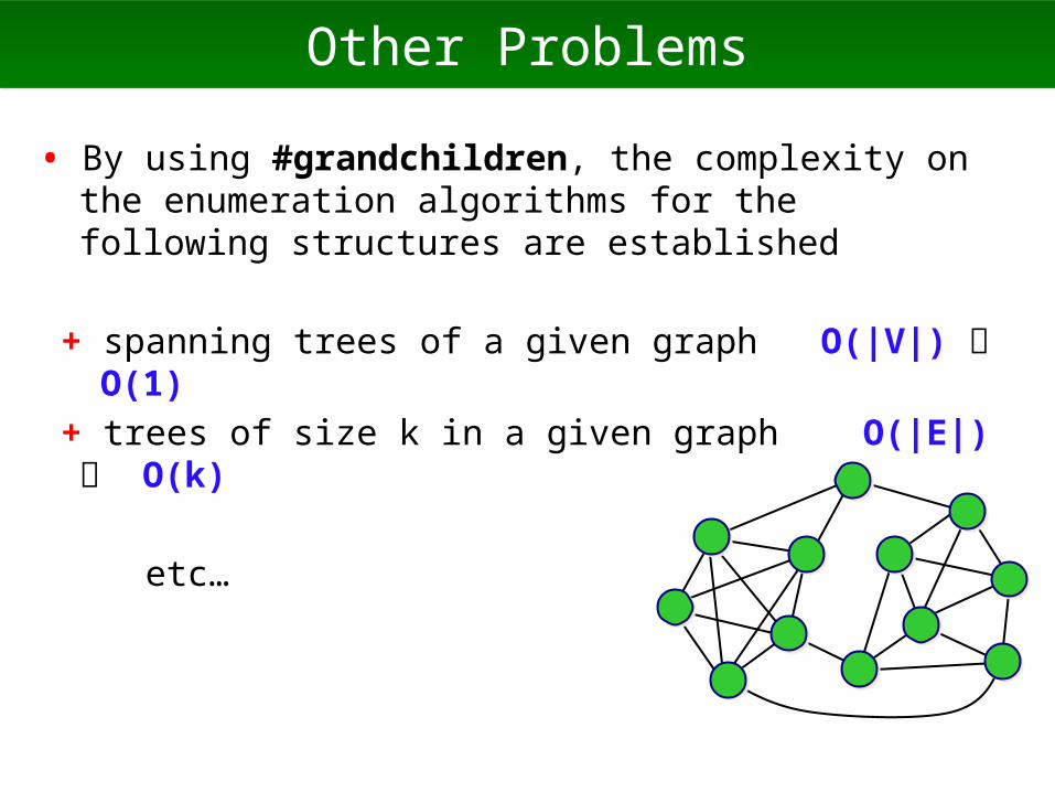
• By using #grandchildren, the complexity on the enumeration algorithms for the following structures are established

+ spanning trees of a given graph O(|V|) O(1)

+ trees of size k in a given graph O(|E|) O(k)

etc…

5 Push out Amortization5 Push out Amortization

Computation Time “Increases”Computation Time “Increases”

• In the “toy” cases, the key property was that

“the total computation time on each level increases with a

constant factor, by going to a deeper level “

2n-(i+1) poly(i+1) / 2n-i poly(i) = poly(i+1) / 2•poly(i)

• It seems that “increase of computation time is good for us”

(it implicitly forbids “sudden decrease”)

• Since the tree is biased, apply this idea locally

--- parent and child (or descendants)

Local IncreaseLocal Increase

• In the “toy” cases, we compare the total computation time on a level and that on the neighboring level

• Instead of that, we compare the computation time of a parent, and the total time on its children

the condition of the toy case is implemented as follows

Σ child Z of X T(Z) ≥ αT(X) for some α > 1

nn-1 n/2

We will characterize good cases by this condition

PO （ Push Out ） ConditionPO （ Push Out ） Condition

T(X): computation time of iteration X

T* : the maximum computation time on a leaf

C(X): set of child iterations of X

α （ T(X) 　≦　　　　 Σ 　T(Y) 　　　　　　　　　　　　　　　　　　　　　　　　　　　 Y C(X)∈

PO Condition

α ， β > 1 constantα ， β > 1 constant

rest ≤ time of children / αrest ≤ time of children / α

FormulaFormula

S(X): computation time given to X by its parent

T* : the maximum computation time on a leaf

C(X): set of child iterations of X

Proof: give one’s computation time to its children, so that each child Z receives (just move, for analysis)

α T(X) × ( T(Z) ／ ΣY C(X)∈ T(Y) )

Each child gives the received time and its own time to its children, recursively (so, grandchildren)

9

4 8

63

if PO condition holds in all iterations, S(X) = O( T(X) ), thus amortized computation time of each iteration is O(T*)

Theorem

Induction Induction

• Each child gives the received computation time and its own computation time to its children (so, grandchildren)

Observation: under this rule, any iteration z receives

at most T(Z) /(α-1) from its parent

(intuitively, T(Z) / α from parent, T(Z) / α2 from grandparent, ... )

• Suppose that an iteration x satisfies the condition

Then, its child z receives at most

{T(Z) / ΣT(Y)} • { T(X) + T(X) / (α-1) }

= {T(Z) / ΣT(Y) } •{ T(X) α / (α-1) }

≤ {T(Z) / α } • { α / (α-1) } 　 = T(Z) / (α-1)

9

4 8

63

9 (α+1) (1/α)

T(X)/ ΣT(Y) ≥ α

Amortized Time on LeafAmortized Time on Leaf

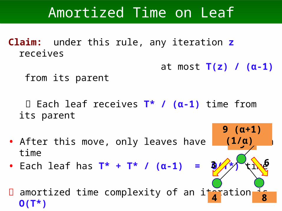
Claim: under this rule, any iteration z receives

at most T(z) / (α-1) from its parent

Each leaf receives T* / (α-1) time from its parent

• After this move, only leaves have computation time

• Each leaf has T* + T* / (α-1) = O(T*) time

amortized time complexity of an iteration is O(T*) 9

4 8

63

9 (α+1) (1/α)

PO （ Push Out ） ConditionPO （ Push Out ） Condition

T(X): computation time of iteration X

T* : the maximum computation time on a leaf

C(X): set of child iterations of X

α （ T(X) － βT* (|C(X)|+1) 　　 ≤ 　　　　 Σ 　 T(Y) 　　　　　　　　　　　　　　　　　　　　　　　　　　　 Y C(X)∈

PO Condition

α ， β > 1 constantα ， β > 1 constantα ， β > 1 constantα ， β > 1 constant

assign T* to it & childrenassign T* to it & children

rest ≤ time of children / αrest ≤ time of children / α

First, for each iteration X, assign T* of its computation time to each child and itself, (βT* (|C(X)|+1) in total), and forget about thisThen, the situation is the same as the previous theorem

FormulaFormula

if PO condition holds in all iterations, the amortized computation time of each iteration is O(T*)

Theorem

PO Condition

T* : the maximum computation time on a leaf

T(X): computation time of iteration X

C(X): set of child iterations of X

S(X): computation time given to X by its parent

α （ T(X) － βT* (|C(X)|+1) 　　 ≤ 　 　 Σ 　 T(Y) 　　　　　　　　　　　　　　　　　　　　　　　　　　　 Y C(X)∈

Connected Component Enumeration

Connected Component Enumeration

Problem: for given a graph G = (V, E), output all vertex sets of G that induces a connected subgraph

In particular, we consider enumeration of

those including a specified vertex r

Connected Component EnumerationConnected Component Enumeration

terms

　 d(v): the degree of v

　 G-v: the graph obtained from G by removing v

　 G/e: the graph obtained from G by contracting edge e

　

AvisFukuda96, U.98

rr

Simple Binary PartitionSimple Binary Partition

• Enumerated by simple binary partition,

with vertex v adjacent to r, as follows

　　● vertex subsets including v

　　　　 recurs with G/(r,v)

　　● vertex subsets not including v

　　　　 recurs with G - v

• An iteration takes O(|V|) time

• PO condition does not hold with naïve observation

rr

vv

Observing in DetailObserving in Detail

• An iteration takes O( d(r) + d(v) ) time, actually

• Child iterations take time

　 Ω( (d(r) + d(v) -2) ／ 2 ＋ ○○ ) and

　 Ω( d(r) -1 ＋ △△ )

● Here, let T(X)= 3d(r)+d(v) and T* = 2

● Sum of child iterations

　 3(d(r)+d(v)-2) ／ 2 + 3d(r)-3

　　　 = 　 ( 9d(r)+3d(v) ) ／ 2 -6 　 ≧ 　 1.5 T(X) – 3T* 　　　　　　　　　　　　　　　　　　　　　　　

rr

vv

Tricky!Tricky!PO condition

holds!PO condition

holds!

Matching Enumeration Matching Enumeration

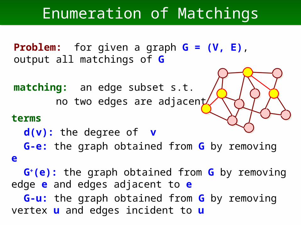
Problem: for given a graph G = (V, E), output all matchings of G

matching: an edge subset s.t.

no two edges are adjacent

Enumeration of MatchingsEnumeration of Matchings

terms

　 d(v): the degree of v

　 G-e: the graph obtained from G by removing e

　 G+(e): the graph obtained from G by removing edge e and edges adjacent to e

　 G-u: the graph obtained from G by removing vertex u and edges incident to u

　

Basic AlgorithmBasic Algorithm

• Matching enumeration is done by, with edge e =(u,v)

　● enumerate matchings including e

recurs with G+(e)

　● enumerate matchings not including e

　 recurs G – (u,v)

that is binary partition (branch & bound)

• An iteration takes O(|V|) time (or maximum degree)

• T* =O(1), but PO doesn’t hold when degrees of u and v are large

vv

uu

…forklore

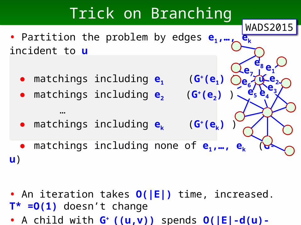
Trick on BranchingTrick on Branching

• Partition the problem by edges e1,…, ek incident to u

　● matchings including e1 (G+(e1) )

　● matchings including e2 (G+(e2) )

　　　　　…　● matchings including ek (G+(ek) )

　● matchings including none of e1,…, ek (G- u)

• An iteration takes O(|E|) time, increased. T* =O(1) doesn’t change

• A child with G+ ((u,v)) spends O(|E|-d(u)-d(v)+1) time, (×d(u))

and the child with G-u spends O(|E|-d(u)) time (×1)

uue1

e2e3e4

e5

e6

e7

e8

WADS2015

PO ConditionPO Condition

• d(u) children spends O(|E|-d(u)-d(v)+1) time, and

a child spends O(|E|-d(u)) time

in total, all children take

O( (d(u)+1) (|E|-d(u)) - Σ d(v) +d(u) )

= O( d(u)(|E|-d(u)) + |E| - Σ d(v) )

= O( d(u)(|E|-d(u)) ) time

• Choosing max. deg vertex as u, then

+ d(u)=1: d(v) is also 1, so two subproblems has ≥ |E|-2 edges

+ d(u) ≥ c|E|: #children ≥ c|E|

+ otherwise: d(u)(|E|-d(u)) ≥ c|E| for some c

• In any case, PO condition hold, thus O(1) time for each

uue1

e2e3e4

e5

e6

e7

e8

Spanning Tree EnumerationSpanning Tree Enumeration

Problem: for a given graph G = (V,E), output all spanning trees of G

Enumeration of Spanning TreesEnumeration of Spanning Trees

terms

　 G-e: the graph obtained from G by removing e

　 G/e: the graph obtained from G by removing edge e and edges adjacent to e

　

WADS2015

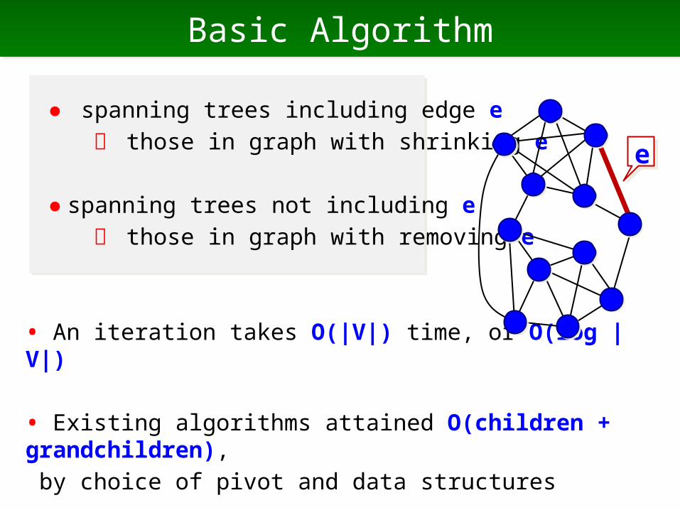
Basic AlgorithmBasic Algorithm

　● spanning trees including edge e

　　　 those in graph with shrinking e

　● spanning trees not including e

　　　 those in graph with removing e

　

• An iteration takes O(|V|) time, or O(log |V|)

• Existing algorithms attained O(children + grandchildren),

by choice of pivot and data structures

ee

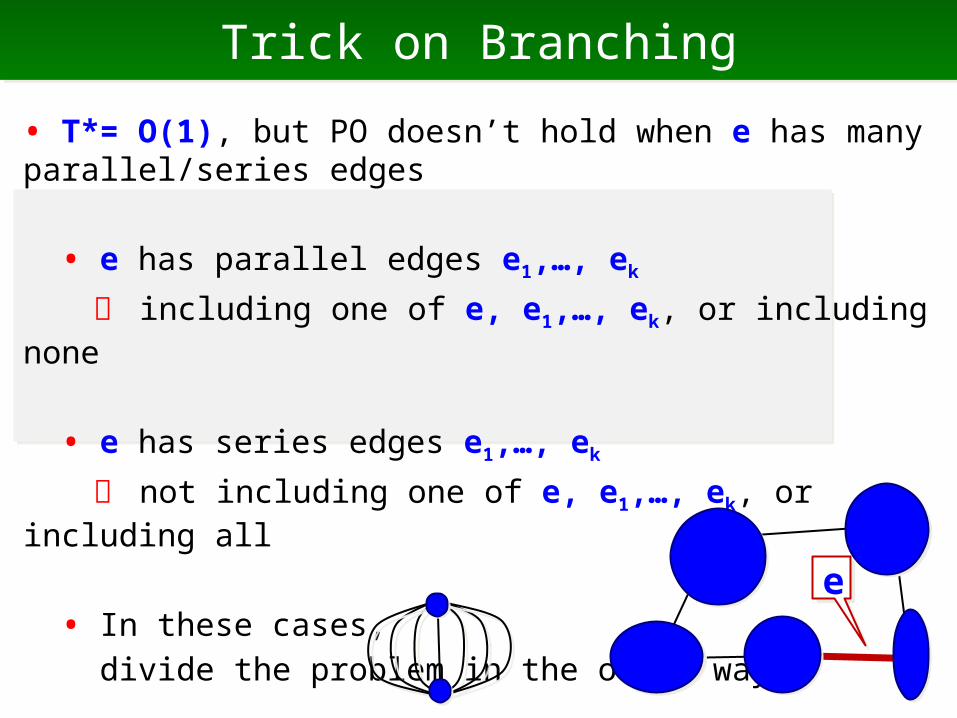
Trick on BranchingTrick on Branching

• T*= O(1), but PO doesn’t hold when e has many parallel/series edges

• e has parallel edges e1,…, ek

　 including one of e, e1,…, ek, or including none

• e has series edges e1,…, ek 　　　 not including one of e, e1,…, ek, or including all

• In these cases,

divide the problem in the other waysee

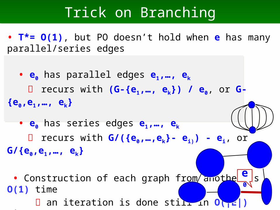
Trick on BranchingTrick on Branching

• T*= O(1), but PO doesn’t hold when e has many parallel/series edges

• e0 has parallel edges e1,…, ek

　 recurs with (G-{e1,…, ek}) / e0, or G-{e0,e1,…, ek}

• e0 has series edges e1,…, ek

　 recurs with G/({e0,…,ek}- ei)) - ei, or G/{e0,e1,…, ek}

• Construction of each graph from another is O(1) time

an iteration is done still in O(|E|) time

• PO condition holds when e has parallel/

series edges so that it has many childrene0e0

Checking PO ConditionChecking PO Condition

• e0 has parallel edges e1,…, ek

　 recurs with (G-{e1,…, ek}) / e0, or G-{e0,e1,…, ek}

• e0 has series edges e1,…, ek

　 recurs with G/({e0,…,ek}- ei)) - ei, or G/{e0,e1,…, ek}

an iteration is done still in O(|E|) time

+ if e0 has < c|E| parallel/series edges,

PO condition holds since children are large

+ if e0 has ≥ c|E| parallel/series edges,

PO condition holds since c|E| children

• So, it is O(1) time for each

e0e0

ConclusionConclusion

ConclusionConclusion

• Mechanism of amortization

- enumeration algorithm spends much time on bottom level

• Basic (toy) case (elimination ordering)

- even toy cases are interesting!

• Local amortization (path enumeration)

- cost for a parent is assigned to children and grandchildren

• Biased (general) case (matching enumeration)

- just modify the algorithm so that the conditions are satisfied

ReferencesReferences PO ConditionT. Uno, Constant Time Enumeration by Amortization, WADS 2015, LNCS9214,

593-605 (2015)

Elimination orderings L. Chandran, L. Ibarra, F. Ruskey, J. Sawada, Generating and characterizing the

perfect elimination orderings of a chordal graph, TCS, 303-317 (2003)

Y. Matsui, T. Uno, On the Enumeration of Bipartite Minimum Edge Colorings, Graph Theory in Paris, Trends in Mathematics 2007, 271-285 (2007)

Matching T. Uno, Algorithms for Enumerating All Perfect, Maximum and Maximal

Matchings in Bipartite Graphs, ISAAC97, LNCS 1350, 92-101 (1997)

T. Uno, A Fast Algorithm for Enumerating Bipartite Perfect Matchings, ISAAC2001, LNCS 2223, 367-379 (2001)

T. Uno, A Fast Algorithm for Enumerating Non-Bipartite Maximal Matchings, J. National Institute of Informatics 3, 89-97 (2001)

ReferencesReferences

Connected component D. Avis, K. Fukuda, Reverse Search for Enumeration, DAM 65, 21-46 (1996)

T. Uno, Studies on Speeding Up Enumeration Algorithms, PhD thesis (1998)

Spanning Trees H. N. Kapoor and H. Ramesh, Algorithms for Generating All Spanning Trees of

Undirected, Directed and Weighted Graphs, LNCS 519, 461-472 (1992)

A. Shioura, A. Tamura and T. Uno, An Optimal Algorithm for Scanning All Spanning Trees of Undirected Graphs, SIAM J. Comp. 26, 678-692 (1997)

T. Uno, An Algorithm for Enumerating All Directed Spanning Trees in a

Directed Graph, ISAAC96, LNCS 1178, 166-173 (1996)

T. Uno, A New Approach for Speeding Up Enumeration Algorithms, ISAAC98, LNCS 1533, 287-296 (1998)

T. Uno, A New Approach for Speeding Up Enumeration Algorithms and Its Application for Matroid Bases, COCOON 99, LNCS 1627, 349-359 (1999)