toward an empirical theory of pulsar emin millisecond ...jmrankin/papers/et_xii.pdf · em is the...

Toward an Empirical Theory of Pulsar Emission. XII. Exploring the Physical Conditionsin Millisecond Pulsar Emission Regions

Joanna M. Rankin1,2 , Anne Archibald2,3 , Jason Hessels2,3 , Joeri van Leeuwen2,3, Dipanjan Mitra1,4,5 , Scott Ransom6 ,Ingrid Stairs7 , Willem van Straten8 , and Joel M. Weisberg9

1 Physics Department, University of Vermont, Burlington, VT 05405, USA; [email protected] Anton Pannekoek Institute for Astronomy, University of Amsterdam, Science Park 904, 1098 XH Amsterdam, The Netherlands

3 ASTRON, the Netherlands Institute for Radio Astronomy, Postbus 2, 7990 AA, Dwingeloo, The Netherlands4 National Centre for Radio Astrophysics, Ganeshkhind, Pune 411 007, India

5 Janusz Gil Institute of Astronomy, University of Zielona Góra, ul. Szafrana 2, 65–516 Zielona Góra, Poland6 National Radio Astronomy Observatory, Charlottesville, VA 29201, USA

7 Physics Department, University of British Columbia, V6T 1Z4, BC, Canada8 Institute for Radio Astronomy & Space Research, Auckland University of Technology, Auckland 1142, New Zealand

9 Physics & Astronomy Department, Carleton College, Northfield, MN 55057, USAReceived 2016 October 13; revised 2017 June 16; accepted 2017 June 19; published 2017 August 9

Abstract

The five-component profile of the 2.7ms pulsar J0337+1715 appears to exhibit the best example to date of acore/double-cone emission-beam structure in a millisecond pulsar (MSP). Moreover, three other MSPs, thebinary pulsars B1913+16, B1953+29, and J1022+1001, seem to exhibit core/single-cone profiles. Theseconfigurations are remarkable and important because it has not been clear whether MSPs and slow pulsarsexhibit similar emission-beam configurations, given that they have considerably smaller magnetospheric sizesand magnetic field strengths. MSPs thus provide an extreme context for studying pulsar radio emission. Particlecurrents along the magnetic polar flux tube connect processes just above the polar cap through the radio-emission region to the light-cylinder and the external environment. In slow pulsars, radio-emission heights aretypically about 500 km around where the magnetic field is nearly dipolar, and estimates of the physicalconditions there point to radiation below the plasma frequency and emission from charged solitons by thecurvature process. We are able to estimate emission heights for the four MSPs and carry out a similar estimationof physical conditions in their much lower emission regions. We find strong evidence that MSPs also radiate bycurvature emission from charged solitons.

Key words: pulsars: general – pulsars: individual (J0337+1715, J1022+1001, B1913+16, B1953+29) –radiation mechanisms: non-thermal

1. Introduction

Millisecond pulsar (MSP) emission processes have remainedenigmatic despite the very prominence of MSPs as indis-pensable tools of contemporary physics and astrophysics. MSPmagnetospheres are much more compact (!100–3000 km), andtheir magnetic field strengths are typically 103–104 timesweaker and probably more complex than those of normalpulsars, which is a result of the period of accretion that isbelieved to recycle old pulsars into MSPs.

Normal pulsars are found to exhibit many regularities ofprofile form and polarization that together suggest an overallbeam geometry comprised by two distinct emission cones and acentral core beam. It would seem that these regularities occur inthe main part because the magnetic field is usually highlydipolar at the roughly 500km height where radio emissionoccurs (J. M. Rankin et al. 2017, in preparation).

The vast majority of MSPs shows no such regularity. Theirpolarized profile forms are often broad and complex and seemalmost a drunken parody of the order that is exhibited by manyslower pulsars (e.g., Dai et al. 2015 and the references therein).The reasons for this disorder are not yet fully clear, but thesmaller magnetospheres of MSPs may well entail emissionheights where the magnetic fields are dominated by quadru-poles and higher terms. In addition, aberration/retardation(hereafter A/R) becomes ever more important for fasterpulsars. In this context, it is arresting to encounter a few

MSPs that appear to exhibit the regular profile forms andperhaps polarization of normal pulsars. If so, even a few suchMSPs provide an opportunity to work out their quantitativeemission geometry and assess whether their radiative processesare similar to those of normal pulsars.The profile of MSP J0337+1715 surprisingly has what

appears to be a five-component core/double-cone configura-tion. Such a five-component structure is potentially importantbecause it has not been clear whether MSPs ever exhibitemission-beam configurations similar to those of slowerpulsars. J0337+1715 is now well known as the uniqueexample so far of an MSP in a system of three stars (Ransomet al. 2014). The pulsar is relatively bright and can beobserved over a large frequency band, so that both its pulsetiming and polarized profile characteristics can be investi-gated in detail.In addition, we find three other probable examples of MSPs

with core-cone profiles: the original binary pulsar, B1913+16;the second MSP discovered, B1953+29; and pulsar J1022+1001. We also discuss the profile geometries of these threeMSPs and consider their interpretations below.The slow pulsars with four-component profiles show outer

and inner pairs of conal components, centered closely on the(unseen) longitude of the magnetic axis, all with particulardimensions relative to the angular size of the pulsar’smagnetic (dipolar) polar cap. The classes of pulsar profilesand their quantitative beaming geometries are discussed in

The Astrophysical Journal, 845:23 (13pp), 2017 August 10 https://doi.org/10.3847/1538-4357/aa7b73© 2017. The American Astronomical Society. All rights reserved.

1

Rankin (1983, hereafter ET I; 1993a, 1993b, hereafter ET VIa& ET VIb) and other population analyses have come to similarconclusions (e.g., Gil et al. 1993 Mitra & Deshpande 1999;Mitra & Rankin 2011). Core beams have intrinsic half-powerangular diameters about equal to a pulsar’s (dipolar) polar cap( n �P2 .45 1 2, where P is the pulsar rotation period), suggestinggeneration at altitudes just above the polar cap. Conal beamradii in slow pulsars also scale as �P 1 2 and reflect emissionfrom heights of several hundred km. Core emission heightsare not usually known apart from the low-altitude implicationof their widths—so it is plausible to assume that coreradiation arises from heights well below that of the conalemission.

Classification of profiles and quantitative geometricalmodeling provides an essential foundation for understandingpulsars physically. MSPs, heretofore, have seemed inexplic-able in these terms. The core/double-cone model works wellfor most pulsars with periods longer than about 100 ms,whereas faster pulsars mostly either present inscrutable singleprofiles or complex profiles where no cones or core can beidentified. It is then important to learn how and why it is thatthe core/double-cone beam model often breaks down for thefaster pulsars.

A/R becomes more important for faster pulsars and MSPssimply because their periods are shorter relative to A/Rtemporal shifts. The role of A/R in pulsar emission profileswas first described by Blaskiewicz et al. (1991, hereafterBCW), but only later was this understanding developed into areliable technique for determining pulsar emission heights (e.g.,Dyks et al. 2004; Dyks 2008; Mitra & Rankin 2011; Kumar &Gangadhara 2012). A/R has the effect of shifting the profileearlier and the polarization-angle (hereafter PPA) traverse laterby equal amounts,

% � o ( )t h c2 , 1em

where hem is the emission height (above the center of the star),such that the magnetic axis longitude remains centered inbetween. In that the PPA inflection is often difficult todetermine, A/R heights have also been estimated by using thecore position as a marker for the magnetic axis longitude,as first suggested by Malov & Suleimanova (1998) andGangadhara & Gupta (2001) and now widely used. The A/Rmethod has thus usually been used to measure conal emissionheights, but core heights have also been estimated for B0329+54 (Mitra et al. 2007) and recently for B1933+16 andseveral other pulsars (Mitra et al. 2016), giving heights aroundor a little lower than the conal heights. Crucially, A/Rmeasurements indicate emission heights of some 300–500 kmin the slow pulsar population. So it is important to seehow MSPs compare, given that many have magnetospheressmaller than 500 km.

In what follows we discuss the observations in Section 2, theJ0337+1715 core component and its width in Section 3.1, andthe conal component configuration in Section 3.2. Section 3.3treats its quantitative geometry, Section 3.4 computes A/Remission heights, and Section 4 considers three other MSPswith cone/single-cone profiles. Finally, Section 5 summarizesthe results, Section 6 interprets them physically, and Section 7outlines the overall conclusions.

2. Observations

2.1. Acquisition and Calibration

J0337+1715. A large number of observations at differentfrequencies and observatories were carried out in the course ofconfirming J0337+1715 and understanding the complex orbitalmodulations of its pulse-arrival times. Some of these werepolarimetric and some much more sensitive, and unsurpris-ingly, the Arecibo observations were usually of the highestquality. In compiling the observations for this analysis, weassessed which observations were deepest at both 1400 and430MHz. The PUPPI backend10 was used at both frequencieswith a 30MHz bandwidth at 430 and a 600MHz bandwidth at1400MHz. We then explored the pulsar’s behavior at higherfrequencies, and both 2.0 and 2.8GHz observations arereported here. We also attempted a rise-to-set observation at5 GHz with a 1GHz bandwidth, but the pulsar was notdetected. All the J0337+1715 observations were calibrated orrecalibrated using the PSRchive pac-x routine (Hotan et al.2004). The final bin size was chosen to reflect the joint timeand frequency resolution, and is given in Table 1 along withsome other characteristics of the observations.The 1391MHz profile in Figure 1 is the deepest and best

resolved of the four and deserves more detailed analysis. The2.8, 2.0, and 0.43 GHz profiles can be seen in Figure 2.B1913+16, B1953+29, and J1022+1001.We also carried

out Arecibo observations of these pulsars using the L-bandWide feed and the Mock11 spectrometers. The former weresingle-pulse polarimetric observations using as many Mockspectrometers as needed to optimize the resolution and use the

Table 1Properties of the Arecibo and GBT Observations

Band Backend MJD Resolution Length(GHz) (°/sample) (s)

J0337+1715(P=2.73 ms; DM=21.32 pc cm!3)1.1–1.7 PUPPI 56736 0.70 "34001.1–1.8 GUPPI 56412 0.70 40,9680.42–0.44 PUPPI 56584 1.41 "34001.9–2.5* PUPPI 56781 1.41 36001.9–2.5 PUPPI 57902 1.41 36002.5–3.1* PUPPI 56768 1.41 39362.5–3.1 PUPPI 57902 1.41 30001.1–1.7 Mocks 56760 4.74 1000B1913+16(P=59.0 ms; DM=168.77 pc cm!3)1.1–1.9 GUPPI 55753 0.35 19001.1–1.7 Mocks 56199 0.58 1200B1953+29(P=6.13 ms; DM=104.501 pc cm!3)1.1–1.6 Mocks 56564 2.24 24001.1–1.6 Mocks 56585 2.24 24001.1–1.9 PUPPI 57129 0.35 3608J1022+1001(P=16.4 ms; DM=10.2521 pc cm!3)1.1–1.7 Mocks 56315/23 0.53 6001.1–1.7 Mocks 56577 0.46 18000.30–0.35 Mocks 56418/31 2.55 6000.30–0.35 Mocks 56577 2.55 1800

Note. These earlier PUPPI 2.0 and 2.8GHz observations could not becalibrated polarimetrically because of faulty cal signals; therefore, we use onlyStokes I in Figure 5.

10 http://www.naic.edu/~astro/guide/node11.html11 http://www.naic.edu/~astro/mock.shtml

2

The Astrophysical Journal, 845:23 (13pp), 2017 August 10 Rankin et al.

total available bandwidth for maximum sensitivity, and theresults are given in Table 1. These Mock observations wereprocessed as described in Mitra et al. (2016), includingderotation to infinite frequency.

2.2. Rotation-measure (RM) Determinations

Our RM determinations will be published as a part of alarger paper in preparation together with a full description ofour observations and techniques.

J0337+1715. A RM of +30±3radm2 was determinedusing a set of the best-quality observations from both theArecibo PUPPI and Green Bank Telescope (hereafter GBT)GUPPI machines.12 These were processed as above withPSRchive, and its rmfit routine was used to estimate each RMand its error; the stated error then reflects the scatter of thesevalues. Ionospheric corrections estimated for these observa-tions ran between +0.8 and –0.2radm2, so the intrinsic valuelies well within the above error. Separately, the Mockobservation of MJD 56760 was used to determine anionosphere-corrected value of +29.3±0.7radm2.

B1913+16.An accurate RM value was determined for thefirst time using five Arecibo Mock 1.4GHz observations—oneof which is shown below in Figure 3. After ionospheric

Figure 1. Total 1.4GHz Arecibo PUPPI polarized profile of pulsar J0337+1715 showing its apparent core component as well as its pairs of inner andouter conal components. The core component seems to be conflated with thetrailing conal components at about 90° longitude. The positions and centers ofthe two conal component pairs are indicated. They are far from symmetricallyspaced as in slower pulsars, apparently because of aberration/retardation.However, note that the outer cone center precedes the inner one as well as thecore. The upper panel gives the total intensity (Stokes I; solid curve), the totallinear ( � �[ ]L Q U2 2 ; dashed green), and the circular polarization (Stokes V;dotted magenta). The PPA [� �( ) ( )]U Q1 2 tan 1 values (lower panel) havebeen Faraday-derotated to infinite frequency. Errors in the PPAs were computedrelative to the off-pulse noise phasor—that is, T T_ � ( )‐ LtanPPA

1off pulse and are

plotted when � n30 and indicated by occasional 3! error bars.

Figure 2. Arecibo PUPPI profiles of J0337+1715 after Figure 1 at higherand lower frequencies than the earlier 1391MHz profile; see Table 1.These show the near absence of evolution with frequency. The profiles,as well as that at 1.4GHz above, are aligned with the dispersive delayremoved.12 https://safe.nrao.edu/wiki/bin/view/CICADA/GUPPiUsersGuide

3


correction, the RMs were estimated by trial and errormaximization of the aggregate linear polarization resulting ina value of +354.4±0.6radm2, where the error reflects therms scatter of the values. This value is then further confirmedby a GBT GUPPI observation, made as part of another project(Force et al. 2015) and processed using the PSRchive rmfitroutine to yield an RM value of +357.9±1.5radm2 thatincluded some 2–3 units of ionospheric contribution. Thisrepresents a substantial increase in precision compared to thecurrent value on the ATNF Pulsar Catalog website of+430±77radm2 (Han et al. 2006).

B1953+29. This RM value was also estimated for the firsttime using Arecibo 1.4GHz observations as processed by boththe Mock spectrometers and PUPPI. The two Mock observa-tions were processed as above and together yielded a value of+3.0±0.4radm2, corrected for ionospheric contributions;the second of the two is shown in Figure 4. In addition, aPUPPI observation was processed as above using PSRchivermfit and yielded a value of +5.7±3.0radm2, which was notcorrected for the expected 2–3 units of ionospheric RM.

J1022+1001.This pulsar has a well-determined RM value of+1.39±0.05radm2 on the ATNF Pulsar Catalog websiteaccording to Noutsos et al. (2015).

3. Exploration of the J0337+1715 Profile

3.1. The Putative Core Feature and its Width

In slower pulsars, the core component width reflects theangular diameter of the polar cap near the stellar surface, and assuch has an intrinsic half-power diameter of n �P2.45 1 2 (P is thestellar rotation period), but the observed width entails a furtherfactor of Bcsc (where α is the colatitude of the magnetic axiswith respect to the rotation axis). The expected intrinsic widthfor this 2.73ms MSP would then be some 47° and theobserved width 67°.5, given that α is plausibly 44° (Ransomet al. 2014) if the orbital and rotational angular momenta arealigned. In J0337+1715!s profile, the putative core is conflatedwith the trailing inner conal component over the entireobservable band, therefore the core width can only then beestimated. Exploratory modeling of the four profiles in theAppendix suggests a core width of between 60° and 70°, so wehave fixed the core width in our modeling at the aboveexpected 67°.5 observed value.

3.2. Double Cone Configuration

In slower pulsars, conal components occur in pairs forinterior sightline traverses where the sightline impact angle C∣ ∣is smaller than the conal beam radius ρ. Geometrically, theseconal component pairs are found to be of two types, inner andouter cones, that have specific (outside, half-power, 1GHz)radii ρ of n �P4 .33 1 2 and n �P5 .75 1 2 (ET VIa, ET VIb; see VIaEquation (4)). In pulsars where both cones and a core areobserved, profiles then have five components, such as in pulsarB1237+25.We suggest that pulsar J0337+1715!s profile in Figure 1

may exhibit just these five components as well as a narrow(putative caustic; see below) feature on the outer edge of the

Figure 3. Arecibo 1.4GHz Mock spectrometer profile of B1913+16 from2012 September 29. The form of this profile differs substantially from thosemeasured earlier (e.g., BCW) because of the star’s precession. Thisobservation was carried out with four Mock spectrometers sampling 86MHzbandwidths and 95 μs resolution. The PPAs have been derotated to infinitefrequency using the measured RM value above, ionosphere corrected, of+354.4±0.4radm2.

Figure 4. Arecibo 1.4GHz Mock spectrometer profile of B1953+29 from2013 October 20. This observation was carried out with seven Mockspectrometers sampling adjacent 34MHz bands with a 38 μs sampling time.Note what appears to be an interpulse preceding the putative core-cone triple(T ) main pulse. We believe this is the first observation to clearly show thepulsar’s PPA traverse and interpulse. The PPAs have been derotated to infinitefrequency using its measured RM of +2.9±0.6radm2 (including some0.8radm2 in the ionosphere). A further Arecibo observation carried out withPUPPI confirms the profile structure and RM value.

4


trailing inner conal component, and we also model thesefeatures in the Appendix. The leading outside (LOC) and insideconal (LIC) components are seen to fall at about !100° and!50° longitude, respectively.

The core is conflated with the trailing conal components(TIC and TOC) at some +100° and +125°, as modeled andbetter estimated in Table 6. The conal components areasymmetric and the rightmost one has a trailing edge bump.However, the Appendix modeling appears to locate theircenters and half-widths adequately. The “spike” on the trailingedge of the trailing inner conal feature above 1 GHz deservesspecial mention, as it seems to resemble the “caustic”13 featuresthat are seen in some other pulsars. The 1391MHz polariza-tion-angle (PPA) traverse shows what seems to be a 90°“jump” at about 135° longitude, and earlier ones at about 50°and 100°; if these are resolved, then the PPA seems to rotaterather little under the components as seems possibly the case atthe other more depolarized frequencies.

3.3. Quantitative Geometry

Profiles for frequencies both higher and lower than that inFigure 1 are given in Figure 2. Note that the pulsar’s fivecomponents can easily be discerned in these profiles up to2.8 GHz and down to 430MHz. The conal features of the430MHz profile are broader and appear less well resolvedcompared to the higher frequency profiles; however, thisappears not to be the result of poorer instrumental resolutionand scattering. The core is obviously conflated with the trailinginner conal component across all the observations, and thismust be taken into account in identifying the structurescontributing to the pulsar’s overall profile.

The centers (C), widths (W) and amplitudes (A) of J0337+1715!s components are given in Table 6, where an effort wasmade to determine these values by fitting methods. However,given the irregular shapes of the components, the fitting errorsare small compared to systematic ones of a few degrees. Thetable thus gives the positions and widths of the conalcomponents so obtained as well as those of the putative“caustic” feature (CC in Table 6) whose center could be fittedwithin about 1°—and it is satisfying to see that this featurealigns in the high frequency profiles within this latter error.Unsurprisingly, the core component properties are moredifficult to estimate in the various profiles, even when takingthe widths as fixed at the expected value as shown in the table.We discuss this further below in connection with the A/Ranalysis where this difficulty is most pertinent.

The properties of the two cones are given in Table 2, wherewi and wo are the inner and outer outside, half-power conalwidths, computed as the longitude interval between thecomponent-pair centers plus half the sum of their widths. Herewe see that the inner and outer conal widths are essentiallyconstant over the observable frequency band. This nearconstancy of profile dimensions over some three octaves issimilar to that observed for other MSPs where there is littlechange in the components separations over the total band ofobservations (e.g., Kondratiev et al. 2016).

Here we apply the standard spherical geometric analysesassuming a central sightline traverse (sightline impact angle !

about 0° as suggested by the relatively constant PPA traverse),that the magnetic colatitude " is 44°, and that the emissionoccurs adjacent to the “last open field lines” (e.g., ET VIa).This analysis is summarized in Table 2, where Si and So are thecomputed conal emission beam radii (to their outside half-power points) per Equation (4) in ET VIa. The emissioncharacteristic heights are then computed assuming dipolarityusing Equation (6).The outside half-power conal radii of about 54° and 75° are

of course enormous compared to those found for slow pulsars.However, they are substantially smaller—only about 2/3—what would be expected according to the slow pulsarrelationships n �P4 .33 1 2 and n �P5 .75 1 2 for the outside 3dBradii of inner and outer cones. The model emission heights ofsome 53 and 100 km are also correspondingly smaller—lessthan half of the 120 and 210 km typically seen in the slowpulsar population. However, it is important to recall that theseare characteristic emission heights, not physical ones,estimated using the convenient but problematic assumptionthat the emission occurs adjacent to the “last open” field lines.It will be interesting to compare these heights with the physicalemission heights estimated using A/R just below.

3.4. A/R Analysis

Here we see that the centers of the outer and inner conalcomponent pairs precede the longitude of the core-componentcenter by some 60° or more—and we propose to interpret thisshift as due to A/R to assess whether the results areappropriate and reasonable. A difficulty is determining theposition of the core component accurately, given its conflationwith the outer conal components. Table 6 below reports theresults of modeling the pulsar’s features with Gaussianfunctions in order to assess the character of this conflationand then estimate the core component’s position and center.Assuming a constant core width at its expected 67°.5 valueand a constant amplitude in relation to the four conalcomponents, the core center falls close to !85° in each bandwithin about 2°. However, other modeling assumptions mightwell yield somewhat different values. We therefore propose totake the core center at !85°±10° in order to incorporate themajor range of estimates and uncertainties. Finally, asemphasized above, core components exhibit a predictablewidth in slow pulsars that reflects both the polar cap geometryand the magnetic colatitude. This is the rationale for holdingthe core width here to its expected value. If, however, J0337

Table 2Double Cone Geometry Model for PSR J0337+1715

Freq wi Si wo So hi ho(MHz) (°) (°) (°) (°) (km) (km)

2800 162 54 238 74 52 992080 163 54 242 74 53 1011391 166 55 240 74 53 99430 163 54 252 76 53 107

Note. wi and wo are the outside half-power inner and outer conal componentwidths scaled from Figures 1 and 2. Si and So are the outside half-power conalbeam radii computed from ET VIa, Equation (4), and hi and ho are therespective geometric conal emission heights computed from the latter paper’sEquation (6) assuming dipolarity and emission along the polar flux-tubeboundary.

13“Caustic” refers to a field-line geometry in which an accidentally favorable

curvature tracks the sightline producing a bright narrow broadband feature(e.g., Dyks & Rudak 2003).

5


+1715, for whatever reason, had a core that was smaller orlarger, then the center would shift by half the differenceamount.

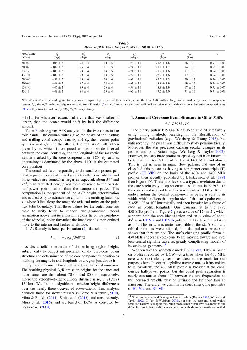
Table 3 below gives A/R analyses for the two cones in thefour bands. The column values give the peaks of the leadingand trailing conal components Gl and Gt, their center pointG G G� �( ) 2c t l , and the offsets. The total A/R shift is thengiven by !, which is computed as the longitude intervalbetween the conal centers Gc and the longitude of the magneticaxis as marked by the core component, or +85°–Gc, and itsuncertainty is dominated by the above±10° in the estimatedcore position.

The conal radii " corresponding to the conal component-pairpeak separations are calculated geometrically as in Table 2, andthose values are somewhat larger as expected, about 54° and75°, than tabulated here, given their reference to the outsidehalf-power points rather than the component peaks. Thiscomputation is independent of the A/R height determinationand is used only to estimate the annuli of the emitting locationss i, where 0 lies along the magnetic axis and unity on the polarflux tube boundary. That these values for the outer cone areclose to unity tends to support our geometrical modelassumption above that its emission regions lie on the peripheryof the (dipolar) polar flux-tube; the inner cone is then emittedmore to the interior and higher in altitude.

In A/R analysis here, per Equation (2), the relation

G� � n ( )h c P 360 2 2em c

provides a reliable estimate of the emitting region height,subject only to correct interpretation of the core-cone beamstructure and determination of the core component’s position asmarking the magnetic axis longitude or a region just above it—in any case at a much lower altitude than the conal emission.The resulting physical A/R emission heights for the inner andouter cones are then about 70 km and 85 km, respectively,where the velocity-of-light-cylinder distance is Rlc Q�( )cP 2130 km. We find no significant emission-height differencesover the nearly three octaves of observations. This analysisparallels those for slower pulsars in Force & Rankin (2010),Mitra & Rankin (2011), Smith et al. (2013), and most recently,Mitra et al. (2016), and are based on BCW as corrected byDyks et al. (2004).

4. Apparent Core-cone Beam Structure in Other MSPs

4.1. B1913+16

The binary pulsar B1913+16 has been studied intensivelyusing timing methods, resulting in the identification ofgravitational radiation (e.g., Weisberg & Huang 2016), butuntil recently, the pulsar was difficult to study polarimetrically.Moreover, the star precesses causing secular changes in itsprofile and polarization (e.g., Weisberg & Taylor 2002).However, its early basic profile morphology had been known tobe tripartite at 430MHz and double at 1400MHz and above.This is just as seen in many slow pulsars, and one of usclassified this pulsar as having a core/inner-cone triple (T )profile (ET VIb) on the basis of the 430- and 1400MHzprofiles then recently published by Blaskiewicz et al. (1991their Figure 17). These profiles show a typical evolution due tothe core’s relatively steep spectrum—such that in B1913+16the core is not resolvable at frequencies above 1 GHz. Key tounderstanding the central component as being a core is itswidth, which reflects the angular size of the star’s polar cap atn �P2 .45 1 2 or 10° intrinsically and then broader by a factor ofBcsc in profile longitude. Our Gaussian fit to the 1990

430MHz profile in Figure 7 gives a value of 17°±2°, whichsupports both the core identification and an # value of about45° as in ET VIa and ET VIb (where the 1GHz width is takenas 14°. This in turn is quite reasonable if the star’s spin andorbital rotations were aligned, but the pulsar’s precessionshows that they are not. The star’s changing profile forms at430MHz suggest a core/cone beam moving toward and everless central sightline traverse, greatly complicating models ofits emission geometry.14

We then take the geometric model in ET VIb, Table 4, basedon profiles reported by BCW—at a time when the 430MHzcore was most clearly seen—as close to the mark for ourpurposes here. Its central sightline traverse makes it insensitiveto $. Similarly, the 430MHz profile is broader at the conaloutside half-power points, but the conal peak separation isnearly constant at about 40° between the two frequencies, sothe increased breadth must be intrinsic and the cone thus aninner one. Therefore, we confirm the core/inner-cone geometryof ET VIa and ET VIb.

Table 3Aberration/Retardation Analysis Results for PSR J0337+1715

Freq/Cone Gil Gi

t Gic Li Si hiem s i

(MHz) (deg) (deg) (deg) (deg) (deg) (km)

2800/II !105±3 124±4 10±5 !75±11 71.5±1.6 86±13 0.91±0.072030/II !102±3 125±4 11±5 !74±11 71.1±1.7 84±13 0.92±0.071391/II !100±3 128±4 14±5 !71±11 71.2±1.6 81±13 0.94±0.07430/II !103±3 129±4 13±5 !72±11 72.2±1.6 82±13 0.94±0.072800/I !51±2 98±4 24±4 !62±11 49.5±1.9 70±12 0.74±0.072030/I !49±2 97±4 24±4 !61±11 48.9±1.9 69±12 0.74±0.071391/I !47±2 99±4 26±4 !59±11 48.9±1.9 67±12 0.75±0.07430/I !48±2 94±4 23±4 !62±11 47.5±2.0 71±13 0.71±0.06

Note. Gil and Gi

t are the leading and trailing conal component positions; Gic their centers; Li are the total A/R shifts in longitude as marked by the core component

centers; h iem the A/R emission heights computed from Equation (2); and Si and s i are the conal radii and emission annuli within the polar flux-tube computed using

ET VIa Equation (4) and S( ) R hsin 2 3i ilc , respectively.

14 Some precession models suggest lower # values (Kramer 1998; Weisberg &Taylor 2002; Clifton & Weisberg 2008), but both the core and conal widthsseem too narrow to support this. Such models incur their own assumptions anddifficulties such that the differences between methods are not easily reconciled.

6


BCW pioneered the use of A/R for determining pulsaremission heights, and their analysis for B1913+16 is illustratedin their Figure 17. They determined the A/R shift from thePPA steepest gradient point (SG) backward to the center of theconal component pair. Arrows in the figures show these points,and according to their analysis, the A/R shift, averagedbetween the two frequencies, is 12°.5±1°.0, which thencorresponds to an emission height of 126±21 km. This in turnthen occurs within a light-cylinder radius of 2820 km.

If the above two points are well identified, the above A/Rvalue follows the method BCW advocated. We can then try toestimate the emission height by two other methods: first, the fitsin Figure 7 clearly show that the core component peak lags thecenter point between the two conal peaks, and this lag is 1°.5 or0.246 ms or some 37 km in altitude per Equation (1)—that is,the conal emission region appears to be higher than the coreregion by this amount. Second, the zero-crossing point ofantisymmetric circular polarization often marks the longitudeof the magnetic axis,15 and in the B1913+16 profile of Figure 3this point falls 6°±1° or some 1.0 ms after the conal centerpoint, suggesting a conal emission height of 148±25 km. Asthe magnetic axis longitude falls halfway between theoppositely shifted profile and PPA traverse under A/R, thelatter result is compatible with BCW’s interpretation and the37km shift may represent the height between the core andconal emission regions.

4.2. B1953+29

The second MSP, B1953+29, also known as Boriakoff’spulsar (Boriakoff et al. 1983), is also a binary pulsar with a117-day orbit. It has also had little subsequent study becausefew profiles have been measured in the intervening decades.Profiles and provisional polarimetry at both 430 and 1400MHzwere presented at an NRAO workshop just after the discovery(Boriakoff et al. 1984), but were not otherwise published, andthe polarimetry efforts appearing since (Thorsett & Stinebring1990; Xilouris et al. 1998; Han et al. 2009; Gonzalez et al.2011) leave many questions unanswered. The pulsar wasdifficult to observe polarimetrically, but Arecibo’s L-bandWide feed together with the Mock spectrometers or PUPPI nowpermit much more sensitive and resolved observations.

The 430 MHz profile described by Boriakoff et al. is single,showing only weak inflections from power in conal outriderson both sides of the broad and relatively intense centralcomponent. At the higher frequency, however, all threecomponents are visible and distinct. This is just the evolutionseen for most conal single (St) pulsars as first described inRankin (ETI, ET VIa). No full beamform computation wasgiven for the pulsar in ETVIb because no reliable polarimetrywas then available.Figure 4 shows a recent Arecibo 1452MHz polarimetric

observation conducted with the Mock spectrometers. It is farmore sensitive and better resolved than any previouslypublished polarimetry for this important pulsar, and clearlyshows its PPA traverse as well as what appears to be a brightinterpulse.16 Again, we have little basis for proceeding with ourinterpretation of the B1953+29 profile unless its putative corecomponent shows an adequate width reflecting that of the polarcap. For this 6.1ms pulsar, the intrinsic core width n �P2 .45 1 2

(ET VIa, Equation (2)) is expected to be some 31°.3. Fits to thecentral component discussed in the Appendix give a width of34°.5 with a fitting error of less than a degree. The larger errorhere, however, is systematic: a Gaussian function may not fitthe core feature well and the adjacent overlapping componentsimply significant correlations. The fitting then indicates a corewidth that is unlikely to be larger than the fitted value butpossibly slightly smaller. Thus there is strong indication thatthis is a core, and that the width reflects a magnetic colatitude—via the Bcsc factor—close to orthogonal, that is, some 65° ormore. The leading feature (preceding the core by about 163°)would then support a nearly orthogonal geometry if indeed thisis an interpulse—and we will make this assumption.17

Now we can also see from Figure 4 that the PPA rate isabout !3°/°. Following the quantitative geometric analysis ofET VIa and ET VIb using the profile dimensions (see theAppendix and Table 7), the results are given in Table 4, wherefor a magnetic colatitude ! of 65° the characteristic emissionheight would be only some 81 km (rather than the 110–120 kmtypical of inner-cone characteristic heights of normal pulsars).An A/R analysis of the B1953+29 profile, assuming that thecore component is at the longitude of the magnetic axis, resultsin the conclusion that the conal center precedes the core by11°±3°, and this in turn corresponds a relative core-coneemission height difference of 27±5 km within a light-cylinderradius of 293 km.

4.3. J1022+1001

PSR J1022+1001, discovered by Camilo et al. (1996), is arecycled MSP with a rotation period of 16 ms. It is in a binarysystem with an orbital periodicity of 7.8 days. The pulsar hasbeen part of several long-term timing programs, but is wellknown to time poorly.18 It has been observed over a broadfrequency band, (e.g., Dai et al. 2015; Noutsos et al. 2015),and below 1 GHz, its profile is clearly comprised of threeprominent components. The underlying PPA traverse has acharacteristic S-shaped RVM form with a “kink” under the

Table 4Conal Geometry Models for B1913+16, B1953+29 and J1022+1001

Pulsar P ! " w # h(ms) (°) (°) (°) (°) (km)

B1913+16 59.0 46 4.0 47 17 126B1953+29 6.1 >65 !18 100 44.4 81J1022+1001 16.4 "60 "7 42 20 45

Note. P, !, and " are the pulsar’s rotation period, magnetic colatitude, andsightline impact angle, respectively. The ws are the outside half-power conalcomponent widths measured from the fitting of Figures 7–9. The #s are theoutside half-power conal beam radii computed from ET VIa, Equation (4), andthe hs are the respective geometric conal emission heights computed from theabove Equation (6) assuming dipolarity and emission along the polar flux-tubeboundary.

15 Core components in slow pulsars often exhibit antisymmetric circularpolarization, such that the zero-crossing point marks the longitude of themagnetic axis. No core is resolvable in Figure 3, but the “bridge” regionbetween the two conal peaks is probably dominated by core emission.

16 This interpulse is also clearly seen in the timing study of Gonzalez et al.(2011)—and hinted at in some of the earlier profiles—and their unpublishedarxiv profile agrees well with ours here.17 The unusual 360° total PPA rotation also suggests an inner (that ispoleward) sightline traverse.18 However, with adequate calibration, the pulsar has recently been shown totime well (van Straten 2013).

7


central component similar to that seen in B0329+54 by Mitraet al. (2007), such that the central slope is some 7°/° (Xilouriset al. 1998; Stairs et al. 1999). Some studies argue that thepulsar exhibits profile changes on short timescales, an effectperhaps similar to mode changing in normal pulsars (seeKramer et al. 1999; Ramachandran & Kramer 2003; Hotanet al. 2004 and Liu et al. 2015). Our three pairs of Areciboobservations at 327 and 1400MHz also suggest slightlydifferent linear and circular polarization at different timeswhile confirming the basic profile structures seen in the abovepapers and the star’s profiles shown here.

In Figure 9 we show Gaussian component fits to J1022+1001 using profiles from Stairs et al. (1999) (Jodrell Bankprofiles downloadable from the European Pulsar Networkdatabase19). We find that these profiles can be decently fittedwith three components, the central one having a width of 17° at610MHz and 14° at 410MHz, roughly close to the polar capsize of 19°. In these fits the location and width of the leadingcomponent are highly correlated and cannot be constrainedvery well, with some effect also on the central component. Thissaid, the effect of A/R in terms of the core center lagging thecenter of the overall profile is clearly seen in this pulsar. Themagnitude of this lag is about 6°.5 at 410MHz and 7° at610MHz, where we find the center of the overall profile basedon the outer Gaussian-fitted component half-power points inTable 7. These estimates place the conal emission at about20 km above the core emission.

In a short communication, Mitra & Seiradakis (2004) usedan A/R model to estimate the emission height across the pulse.They argued that the pulsar could be interpreted in terms of acentral core and a conal component pair as shown in theirFigure 2. They found a slight difference in emission heightbetween the core and conal emission, which then had the effectdue to A/R of inserting a kink in the PPA traverse similar towhat is observed. For this to happen, they suggest that the coreemission originates closer to the neutron star surface, and theconal emission region is then about 25 km above that of thecore emission, similar to estimates obtained from the profileanalysis mentioned above.

5. Summary of Observational Results

MSP J0337+1715 apparently provides a rare opportunity tostudy a core/double-cone emission beam configuration in therecycled and relatively weak magnetic field system of an MSP.Slow pulsars with five-component profiles showing the coreand both conal beams are unusual—because our sightline mustpass close to the magnetic axis to encounter the core andresolve the inner cone—but such stars exhibit the mostcomplex beamforms that pulsars normally seem capable ofproducing.

The conal dimensions of J0337+1715 and A/R analysisprovide a novel and consistent picture of the emission regionsin this MSP. The A/R analysis argues that the inner conalemission is generated at a height of some 70 km and the outercone then at about 85 km, and adjustment of the quantitativegeometry for the estimated sL values provides roughlycompatible emission heights. No evidence of conal spreadingis seen over the nearly three octave band of observations, againsuggesting that all the emission is produced within a narrowrange of heights.

Questions have remained about whether MSPs radiate inbeamforms similar to those of slower pulsars. When putativecore components have been seen in MSPs—as in the roughlyfive-componented profiles of J0437–4715—they are usuallynarrower than the polar-cap angular diameter and thus cannotbe core emission features in the manner known from the slowpulsar population. This might be because MSP magneticdipoles are not centered in the star, which in turn might resultfrom the field destruction during their accretional spinup phase(e.g., Ruderman 1991). Or conversely, perhaps in J0337+1715this field destruction was more orderly or less disruptive than inmany other MSPs.Core/cone beam structure had heretofore been identified in a

few MSPs—B1913+16, B1953+29, and J1022+1001—andnot systematically assessed in these until recently because theavailable polarimetry made quantitative geometric modelingdifficult and inconclusive. Here we have been able to carry outsuch analyses that argue strongly for core/cone structure inthese three other MSPs. In each case, we find core widths thatare compatible with the full angular size of their (dipolar) polarcaps at the surface. We further find characteristic emissionheights for these pulsars that are all smaller or much smallerthan expected for the inner cones of normal pulsars. A/Ranalyses then provide more physical emission heights: ForB1913+16, a 59ms MSP with the largest light-cylinder of2820 km, its properties are most like those of slow pulsar innercones. For each of the other three, however, with much fasterrotations and smaller magnetospheres, both the quantitativegeometry and A/R analyses indicate radio emission from loweraltitudes of only a few stellar radii.These results can embolden us to recognize core/cone

structure in other MSPs, classify them, and study their emissiongeometry quantitatively in order to determine if, in fact, somefew other core/cone profiles can be recognized among themany MSPs with inscrutable ones. These results underscorethat while the few MSPs here seem to exhibit such structure,many or most appear not to. Thus these results may begin toprovide a foundation for exploring the consequences ofaccretional magnetic field destruction during MSP spinup. Itmay well be that orderly core/cone beam structure signals anddepends on a nearly dipolar magnetic field configuration at theheight of the radio-emission regions (J. M. Rankin et al. 2017,in preparation). Therefore, for reasons to be learned in thefuture, some MSPs may be able to retain a sufficientlydominant dipolar magnetic field in their radio emission regionsdespite its dramatic weakening by accretion—whereas mostother MSPs apparently do not.

6. Physical Analysis of Emission-region Conditions

Other recent A/R analyses of slower pulsars (e.g., Mitraet al. 2016 and references therein), and theoretical develop-ments (e.g., Gil et al. 2004; Melikidze et al. 2014 andreferences therein) strongly argue that the radio emission inslower pulsars comes from altitudes of about 500 km. By thenestimating the magnetic field strength, the Goldreich-Julian(1969) plasma density 8 Q� · Bn c2GJ (rotational frequency

Q8 � P2 , B is the magnetic field, and c the light speed), andthe plasma, cyclotron, and curvature frequencies at theseheights of emission, we are able to show that the radiationemerges from regions where the three latter frequencies are allmuch greater than the frequency of the emitted radiation. Thisindicates that the mechanism of radiation must be the curvature19 http://www.epta.eu.org/epndb/

8


process and the emitting entities charged solitons (e.g., Mitraet al. 2009, 2015, 2016; Mitra & Rankin 2017), which inturn connects with constraints on the physical propagationmodes (ordinary, extraordinary) of the observed radiation(Rankin 2015).

We then here assess the results of a similar modeling of thephysical properties of the emission regions in the four MSPsstudied above. A summary of the estimated plasma properties foreach MSP at its A/R-determined emission height is given inTable 5.20 The cyclotron frequency OB is estimated for asecondary plasma Lorentz factor Hs of 200. The plasma frequencyOp is estimated for H � 200s and two values of the overdensityL � n ns GJ of 100 and 104, and the curvature frequency Ocr fortwo values of ( � 300, 600s , the Lorentz factor of the emittingsoliton. The radius of the light cylinder is given by Q�R cP 2lc ,and the model height of the radio emission r in terms of light-cylinder distance is given by �R r Rlc.

The Table 5 values show that the radio frequency is far lowerthan conservative estimates of the cyclotron, plasma, andcurvature frequencies in every case. This in turn demonstratesnot only that MSP emission functions physically in a manner thatis very similar or identical to slower pulsars, but it also indicatesthat the mechanism of radiation must be the curvature process andthe emitting entities charged solitons as in slower pulsars (Mitraet al. 2016). Very similar conclusions can be reached via theconclusion that the 22.7ms pulsar J0737–3039A has an emissionheight of some 9–15 stellar radii (Perera et al. 2014).

7. Conclusions

MSP J0337+1715 together with the other three pulsarsstudied above apparently show us that some MSPs are capableof core/(double)-cone emission—and thus that the engines ofemission in MSPs are not essentially different than those inslower pulsars. In particular, we have been able to estimate theemission heights of the four MSPs using both geometricmodeling and A/R, and all indicate that the emission regionslie deep within the larger polar flux tubes of their shallowermagnetospheres. We also find as for the slower pulsars that intheir radio emission regions the cyclotron, plasma, andcurvature-radiation frequencies are much higher than those of

the emitted radiation, strongly arguing for the curvatureemission process by charged solitons.

We thank Paul Demorest for assistance in analyzing a GreenBank Telescope observation of B1913+16 and Michael Kramerfor use of his bfit code. Much of the work was made possible bysupport from the US National Science Foundation grant 09-68296as well as NASA Space Grants. One of us (J.M.R.) also thanks theAnton Pannekoek Astronomical Institute of the University ofAmsterdam for their NWO Vidi/Aspasia grant (PI Watts) support.Another (J.v.L.) thanks the European Research Council forfunding under Grant Agreement n. 617199. J.M.W. was supportedby NSF Grant AST 1312843 Arecibo Observatory is operated bySRI International under a cooperative agreement with the USNational Science Foundation, and in alliance with SRI, the Ana G.Méndez-Universidad Metropolitana, and the Universities SpaceResearch Association. The National Radio Astronomy Observa-tory is a facility of the National Science Foundation operatedunder cooperative agreement by Associated Universities, Inc. Thiswork made use of the NASA ADS astronomical data system.

AppendixResults of Profile Modeling

A.1. J0337+1715

In order to intercompare our analyses in the four bandsconveniently, they should be well aligned in time. An attemptwas made to align the profiles according to their timing anddispersion delay, which was roughly satisfactory (except for the2.0GHz band, which was found to be early by about 10°, andthe 430MHz band, which was late by about 5°. Theadjustments brought the centers of the putative “caustic”features into close alignment, as can be seen in the models ofTable 6, and Figure 6 is a check on the Arecibo polarimetry.Figure 5 shows the 1391MHz and other profiles with the

various model components. Similar modeling efforts werecarried out for each of the profiles, and the results are tabulatedin Table 6. The inner and outer cones and core are modeledwith Gaussian components, and one further Gaussian is used tomodel the putative caustic component on the trailing edge ofthe trailing inner conal component. The leading conalcomponents then align within an rms of about a degree, andthe trailing ones about twice that. Clearly, the Gaussianfunctions model the profile components only poorly. Mostcomponents have complex and asymmetric shapes, and the

Table 5Summary of Plasma Properties for MSP Radiation

Pulsar P P Beamform Oobs h OB Op Ocr R Rlc

(ms) (10!20 s s!1) (GHz) (km) (GHz) (GHz) (GHz) (km)

J0337+1715 2.732 1.76 Inner Cone 1.4 69 19 15!146 11!87 0.53 130Outer Cone 1.4 83 11 11!111 10!79 0.64 130

B1913+16 59.0 86 Inner Cone 1.4 126 101 7!73 2!14 0.04 2817

B1953+19 6.13 2.97 Inner Cone 1.4 27 614 55!555 12!93 0.09 29381 23 11–107 7–54 0.28 293

J1022+1001 16.4 4.3 Inner Cone 1.4 25 1530 53!535 7!59 0.03 78645 262 22–221 5–44 0.06 786

Note. The frequency OB is the cyclotron frequency estimated for H � 200s , frequency Op estimated for H � 200s and two values of L � 100, 104, and the cyclotronfrequency estimated for two values of ( � 300, 600s . Italicized values follow from the geometric model (characteristic) heights in Table 4.

20 Values are also given in italics for B1953+29 and J1022+1001corresponding to the geometric model (characteristic) heights in Table 4,where the A/R height may only measure the difference between the core andconal emission heights.

9


fitting results seem adequate only to estimate the widths andcenters of the five components approximately.

However, it is the center of the core component that in principlefalls close to the magnetic axis, but this point can only beestimated by modeling due to the conflation of the core with thetrailing components. In particular, the Gaussian model for the corecomponent’s shape at 1391MHz is clearly poor. The modelingefforts do show that the space is adequate before and below thetrailing components for a core of the expected 67°.5 half-width.Recent evidence indicates that some cores may have an unresolveddouble form, and a model using two Gaussians of half theexpected width and separated by this half-width does model the1391MHz feature somewhat better (dashed magenta curve).

The Gaussian component modeling of the estimated corecenters gives reasonably consistent results for the four bands, asseen again in Figure 5 and Table 6. In each case, the core widthwas fixed at its expected 67°.5 value, and its amplitude was alsoadjusted to be about 15% of the two leading conal component’samplitudes in order to control the correlation of its amplitudewith that of the trailing inner conal component. Within theseassumptions, the estimated core center position falls at +85°±2°longitude. However, the probable errors are much larger. The A/R analysis above uses the differences between the conalcomponent centers and the core center. We have seen that themodel differences across the bands of a conal component centerare only one or two degrees; however, a different modelingassumption might shift the core center by a larger amount. Wetherefore propose to adopt a core center value of +85°±10° toaccommodate these various uncertainties.

A.2. B1913+16

The binary pulsar B1913+16 can no longer be observed toclearly show its three components and putative core-conestructure at frequencies around 430MHz. Its secularly chan-ging profiles show that its emission beam is precessing, shiftingthe orientation of our sightline’s traverse through it, such that

Table 6J0337+1715 Component Modeling Summary

LOC LIC Core TIC TOC “CC”

1.4GHz BandC (°) !100 !47 83 99 128 110W (°) 17 18 67.5 20 12 3.5A 82.0 17.6 14.0 23.1 45.7 14.0

2.8GHz BandC (°) !105 !51 87 98 124 109W (°) 19 14 67.5 14 8 4.7A 0.20 0.06 0.04 0.08 0.10 0.15

2.0GHz BandC (°) !102 !49 87 97 125 110W (°) 16 16 67.5 17 13 5.8A 13.5 3.0 2.2 4.2 5.8 6.0

327MHz BandC (°) !103 !48 84 94 129 LW (°) 19 19 67.5 24 21 LA 940 498 179 150 500 L

Note. “LOC/LIC” leading inner/outer cones; “TIC/TOC” trailing inner/outercones; and “CC” caustic component. “C” center; “W” half-power width; and“A” amplitude.

Figure 5. Total power profiles of J0337+1715 as in Figures 1 and 2, showingthe several Gaussian functions used to model the profiles and estimate thecenters and dimensions of the components in Tables2, 3, and 6. The outerconal Gaussian functions are shown as a dashed blue line, the inner as a dashedgreen line, and the core as a solid magenta line—and the caustic feature isplotted as a dashed cyan line. An unresolved double model is also shown forthe 1391MHz profile (dashed magenta); see text. The model dimensions aregiven in Table 6.

10


eventually, its beam will no longer point in our direction(Weisberg & Taylor 2002). Therefore, we make use hereof both archival and current observations. Please refer to thewell-measured Arecibo profiles of Blaskiewicz et al. (1991;their Figure 17); Figure 3 gives a current Arecibo 1390MHzprofile; and we use another archival Arecibo observation inFigure 7 to determine the centers and widths of its three profilecomponents by Gaussian fitting.

The fitting results are given in Table 7. Here the Gaussian fitsworked well as can be seen in the figure, implying that here thethree components can be closely modeled using Gaussianfunctions. These dimensions are used above to assess the half-power width of the central components so as to vet it as a corecomponent, and in Table 4 to quantify the geometry of thepulsar’s cone after ET VIa and ET VIb.

A.3. B1953+29

Similar Gaussian fitting was carried out for MSP B1953+29using the 1452MHz Arecibo observation in Figure 3 above.The results of the fits for the three profile components andpossible interpulse are shown in Figure 8, where it is clear thatthe modeling was again successful in this case. Gaussianfunctions fit all four profile features well, and their fitted centersand widths are again given in Table 7. The results are also usedabove to assess whether the core width is compatible with a

Figure 6. Total 1.4GHz Green Bank Telescope GUPPI profile of pulsar J0337+1715 as in Figure 1. The profiles compare well with each other, despiteconcerns that the polarization might be distorted by reflections for a source thatmust be tracked at Arecibo fully under its triangular supporting structure. TheGreen Bank Telescope is designed to avoid all such issues. Arecibo’s PUPPIand the latter’s GUPPI are almost identical instruments.

Figure 7. Arecibo 430MHz profile of B1913+16 from 1990 August 18showing the three Gaussian functions used to fit the profile and estimate thecenters and dimensions of the components in Tables 4 and 7. The conalGaussian functions are shown as a green line, and the central core is plotted asa red line. The baseline ripples on the leading edge may result frominterference.

Table 7Component Fitting Summary for Pulsars B1913+16, B1953+29, and

J1022+1001

Pulsar LC Core TC IP(GHz) (°) (°) (°) (°)

B1913+16 C !23.8 !2.8 15.8 LW 13.6 16.6 15.0 LA 0.06 0.03 0.05 L

B1953+29 C !52.2 !2.8 15.5 !165.6W 13.6 16.6 15.0 25.9A 132e3 55e3 81e3 9e3

J1022+1001410 MHz C !12.5 0.4 12.5 L

W 27.9 13.6 6.0 LA 0.34 0.77 0.73 L

610 MHz C !15.3 3.4 15.1 LW 18.9 17.8 5.4 LA 0.15 0.59 0.78 L

Figure 8. Total power profile of B1953+29 at 1452 MHz as in Figure 3,showing the several Gaussian functions used to fit the profile and estimate thecenters and dimensions of the components in Tables4 and 7. The conalGaussian functions are shown as a green line, and the central core is plotted asa red line.

11


core identification and to provide an analysis of the conal beamgeometry in Table 4.

A.4. J1022+1001

We also studied the profiles of pulsar J1022+1001. Theresults of the two fits for the pulsar’s three profile componentsare given in Figure 9. Gaussian functions fit the three profilefeatures well, and their fitted centers and widths are again givenin Table 7. Kramer et al. (1999) fitted the overall pulsar profileat 1.4 GHz with five Gaussian components, and the star’sprofile does exhibit a narrow “cap”-like feature at 1 GHz andabove somewhat similar to the caustic profile of J0337+1715.Indeed, our observations show that the relative intensity of thisnarrow “cap” feature increases very rapidly with frequencyfrom being undetectable at meter wavelengths, just so at 1 GHz

and dominant at 1.7 GHz. The alignment of the meter andcentimeter profiles is very nicely shown in the recent paper byNoutsos et al. (2015; Figure 11). We therefore conclude that itsbehavior is unlike anything previously seen in cores and can beignored for the present purposes. The results are also usedabove to assess whether the core width is compatible with acore identification and to provide a quantitative analysis of theconal beam geometry in Table 4.

ORCID iDs

Joanna M. Rankin https://orcid.org/0000-0002-8923-6065Anne Archibald https://orcid.org/0000-0003-0638-3340Jason Hessels https://orcid.org/0000-0003-2317-1446Dipanjan Mitra https://orcid.org/0000-0002-7653-8494Scott Ransom https://orcid.org/0000-0001-5799-9714Ingrid Stairs https://orcid.org/0000-0001-9784-8670Willem van Straten https://orcid.org/0000-0003-2519-7375Joel M. Weisberg https://orcid.org/0000-0001-9096-6543

References

Blaskiewicz, M., Cordes, J. M., & Wasserman, I. 1991, ApJ, 370, 643Boriakoff, V., Buccheri, R., & Fauci, F. 1983, Natur, 304, 417Boriakoff, V., Stinebring, V., et al. 1984, NRAO Workshop 8Camilo, F., Nice, D. J., Shrauner, J. A., & Taylor, J. H. 1996, ApJ, 469,

819Clifton, T., & Weisberg, J. M. 2008, ApJ, 689, 687Dai, S., Hobbs, G., Manchester, R. N., et al. 2015, MNRAS, 449, 3223Dyks, J. 2008, MNRAS, 391, 859Dyks, J., & Rudak, B. 2003, ApJ, 598, 1201Dyks, J., Rudak, B., & Harding, A. K. 2004, ApJ, 607, 939Force, M. M., Demorest, P., & Rankin, J. M. 2015, MNRAS, 453, 4485Force, M. M., & Rankin, J. M. 2010, MNRAS, 406, 237Gangadhara, R. T., & Gupta, Y. 2001, ApJ, 555, 31Gil, J., Lyubarski, Y., & Melikidze, G. I. 2004, ApJ, 600, 872Gil, J. A., Kijak, J., & Seiradakis, J. M. 1993, A&A, 272, 268Goldreich, P., & Julian, W. H. 1969, ApJ, 157, 869Gonzalez, M. E., Stairs, I. H., Ferdman, R. D., et al. 2011, ApJ, 743, 102Han, J. L., Demorest, P. B., van Straten, W., & Lyne, A. G. 2009, ApJS,

181, 558Han, J. L., Manchester, R. N., Lyne, A. G., Qiao, G. J., & van Straten, W.

2006, ApJ, 642, 868Hotan, A. W., Bailes, M., & Ord, S. M. 2004, MNRAS, 355, 941Hotan, A. W., van Straten, W., & Manchester, R. N. 2004, PASA, 21,

302Kondratiev, V. I., Verbiest, J. P. W., Hessels, J. W. T., et al. 2016, A&A,

585, 128Kramer, M. 1998, ApJ, 509, 856Kramer, M., Xilouris, K. M., Camilo, F., et al. 1999, ApJ, 520, 324Kumar, D., & Gangadhara, R. T. 2012, ApJ, 746, 157Liu, K., Karuppusamy, R., Lee, K. J., et al. 2015, MNRAS, 449, 1158Malov, I. F., & Suleimanova, S. A. 1998, ARep, 42, 388Melikidze, G. I., Mitra, D., & Gil, J. 2014, ApJ, 794, 105Mitra, D., & Deshpande, A. A. 1999, A&A, 346, 906Mitra, D., Gil, J., & Melikidze, G. I. 2009, ApJ, 794, 105Mitra, D., Melikidze, G. I., & Gil, J. 2015, in ASI Conf. Ser. 12, Recent Trends

in the Study of Compact Objects (RETCO-II): Theory and Observation, ed.I. Chattopadhyay et al. (Bangalore: ASI), 43

Mitra, D., & Rankin, J. M. 2011, ApJ, 792, 92Mitra, D., & Rankin, J. M. 2017, MNRAS, 468, 4061Mitra, D., Rankin, J. M., & Arjunwadkar, M. 2016, MNRAS, 460, 3063Mitra, D., Rankin, J. M., & Gupta, Y. 2007, MNRAS, 379, 932Mitra, D., & Seiradakis, J. M. 2004, arXiv:astro-ph/0401335Noutsos, A., Sobey, C., Kondratiev, V. I., & Weltevrede, P. 2015, A&A,

576, A62Perera, B. B. P., Kim, C., McLaughlin, M. A., et al. 2014, ApJ, 787, 51Ramachandran, R., & Kramer, M. 2003, A&A, 407, 1085Rankin, J. M. 1983, ApJ, 274, 33 (ET I)Rankin, J. M. 1993a, ApJ, 405, 285 (ET VIa)Rankin, J. M. 1993b, ApJS, 85, 145 (ET VIb)Rankin, J. M. 2015, ApJ, 804, 112

Figure 9. Total power profiles of J1022+1001 at 410 MHz (upper panel) and610 MHz (lower panel) from Jodrell Bank Observatory, showing the severalGaussian functions used to fit the profile and estimate the centers anddimensions of the components in Tables4 and 7. The conal Gaussian functionsare shown as a green line, and the central core is plotted as a red line.

12


Ransom, S. M., Stairs, I. H., Archibald, A. M., Hessels, J. W. T., et al. 2014,Natur, 505, 520

Ruderman, M. A. 1991, ApJ, 382, 587Smith, E. M., Rankin, J. M., & Mitra, D. 2013, MNRAS, 435, 1984Stairs, I. H., Thorsett, S. E., & Camilo, F. 1999, ApJS, 123, 627Thorsett, S. E., & Stinebring, D. R. 1990, ApJ, 361, 644

van Straten, W. 2013, ApJS, 204, 13Weisberg, J. M., & Huang, Y. 2016, ApJ, 829, 55Weisberg, J. M., & Taylor, J. H. 2002, ApJ, 576, 942Xilouris, K. M., Kramer, M., Jessner, A., et al. 1998, ApJ, 501, 286Yan, W. M., Manchester, R. N., & van Straten, W. 2011, MNRAS, 414,

2087

13


toward an empirical theory of pulsar emin millisecond ...jmrankin/papers/et_xii.pdf · em is the...

Documents