tourism, trade and wealth accumulation with …
TRANSCRIPT

ECOFORUM
[Volume 4, Issue 1 (6), 2015]
7
Wei-Bin. ZHANG
Ritsumeikan Asia Pacific University, Japan
wbz1 @apu.ac.jp
Abstract
The purpose of this study is to study dynamic interactions among economic growth, structural change, international
trade and tourist flows. It builds a multi-country growth model with endogenous wealth accumulation and tourism.
The model is unique in that it introduces endogenous tourism within a general dynamic equilibrium framework. The
model is built on microeconomic foundations. It not only integrates the three well-known Solow growth model,
Oniki-Uzawa trade model, and the Uzawa two-sector model, but also introduces tourist flows between economies for
any number of national economies. After building the model, we demonstrate that the motion of the J -country world
economy can be described by J differential equations. We also simulate the global economy with three countries,
showing that the world dynamics has a unique equilibrium. We carry out comparative dynamic analysis with regard
to one country's total productivity factor, the propensity to save, the propensity to tour other countries, and the
population.
Key words: trade pattern; tourism; services; growth; wealth accumulation; income and wealth distribution among
countries.
JEL Classification: F11; O41; L83
I.INTRODUCTION
This study proposes a multi-country growth model with international trade and economic structures. The
growth mechanism is based on the Solow growth model and ideas of possible mutual benefits from free trade. In
describing each country's economic structure we base our study on the Uzawa tow-sector growth. We describe trade
and trade pattern determination on the basis of Oniki and Uzawa and others (for instance, Oniki and Uzawa, 1965;
Frenkel and Razin, 1987; Nishimura and Shimomura, 2002; and Sorger, 2002). The Oniki-Uzawa model deals with
a two-country world economy with two goods. The Oniki-Uzawa modelling framework is now often applied to study
dynamic interdependence between trade patterns and economic growth. In the literature of trade and growth there
some other trade models which make systematic treatments of wealth accumulation in the context of international
economics. Most of trade models with endogenous wealth are either limited to two-country or small open economies.
The model in this study is for any number of national economies, each national economy supplying internationally
tradable goods and domestic services (which can be consumed by foreign tourists). It is a dynamic general
equilibrium model, treating the global economy as an integrated whole.
A unique feature of this study is introduction of tourism into a dynamic general equilibrium model. Tourism
has played increasingly important role in national economies partly due to rapid economic globalization and
economic growth in different parts of the world. It is obvious that tourism has interdependent relations with
economic growth and other economic activities. As far as trade is concerned, tourism is special in that it converts
some non-traded goods into tradable ones. Tourism goods such as monuments of national heritage, historical sites,
beaches, and hot springs, are not-tradable as their consumption is at the same location. People from other regions can
enjoy the goods only by visiting the spot. Tourism affects local economies in different ways. On the one hand,
tourism attracts resources such as labor and capital from other sectors of the economy and, on the other hand, the
income generated by tourism encourages development of other economic activities. Foreign tourism is an
important source of income and employment in some economies (Sinclair, 2002; Lee and Chang, 2008; Schubert
et al., 2011; Seentanah, 2011; Sun, 2014). This study examines dynamic interdependence between tourism, trade
and growth in a general equilibrium framework. Tourism has caused increasingly more attention in the literature of
economics (e.g., Sinclair and Stabler, 1997; Hazari and Sgro, 2004; and Hazari and Lin, 2011). According to Chao et
al. (2009) the study of tourism has been mainly static. It is necessary to build dynamic models on microeconomic
foundation. Another important issue is related to economic structural changes with tourism. As tourism uses national
resources, development of tourism affects economic structure (e.g., Corden and Neary, 1982; Copeland, 1991; Oh,
2005; Zeng and Zhu, 2011). In order to fully understand possible effects of tourism on national economic
development and economic structure, it is necessary to build a dynamic general equilibrium framework. Dwyer et al.
TOURISM, TRADE AND WEALTH ACCUMULATION WITH ENDOGENOUS
INCOME AND WEALTH DISTRIBUTION AMONG COUNTRIES

ECOFORUM
[Volume 4, Issue 1 (6), 2015]
8
(2004) discuss the need for dynamic general equilibrium modeling when studying tourism and its interaction
with the rest economy. Blake et al. (2006) also address the issue. Nevertheless, there are a few dynamic economic
models of dynamic interdependence between economic growth and tourism with micro-behavioral foundation. This
study studies tourism and economic growth on basis of Uzawa’s two-sector growth model (Uzawa, 1963; Galor,
1992; Mino, 1996; Cremers, 2006; Li and Lin, 2008; and Stockman, 2009).
This study applies an alternative approach to household behavior proposed by Zhang (1993). It is based on
the two models recently proposed by Zhang (2012a, 2012b). Zhang (2012a) builds a multi-country trade model
with wealth accumulation and economic structure. Nevertheless, the model does not take account of tourism.
This study introduces tourism into this model by following Zhang (2012b) in describing behavior of tourists
taking account of modelling. Different from Zhang (2012b) which is for small-open economies, this study treats
tourism within a general equilibrium framework. The rest of the paper is organized as follows. Section 2 defines
the basic model. Section 3 shows how we solve the dynamics and simulates the motion of the global economy.
Section 4 carries out comparative dynamic analysis to examine the impact of changes in some parameters on the
motion of the global economy. Section 5 concludes the study. The appendix proves the main results in Section 3.
II.THE MODEL
We use the Uzawa two-sector growth model to describe national economies. Most of the models in the
neoclassical growth theory model are extensions and generalizations of the pioneering works of Solow (1956). The
model has been extended and generalized in numerous directions (e.g., Diamond, 1965; Stiglitz, 1967; Burmeister
and Dobell, 1970; Benhabib et al. 2000; Drugeon and Venditti, 2001; and Ortigueira and Santos, 2002). An
important extension was initiated by Uzawa (1961), who made an extension of Solow’s one-sector economy by a
breakdown of the productive system into two sectors using capital and labor, one of which produces industrial goods,
the other consumption goods. But all these studies do not have tourism. This study structurally generalizes the Uzawa
two-sector model to include tourism. Determination of international trade pattern in our approach is based the Oniki-
Uzawa model (see also, Brecher, et al., 2002; Sorger, 2002). It is assumed that the countries produce a homogenous
tradable commodity (see also Ikeda and Ono, 1992). There is only one (durable) good in the global economy and one
(national) services and consumer goods under consideration. Domestic households consume both goods, while
foreign tourists consume only services. It is assumed for analytical simplicity that tourists do not consume traded
goods. Tourism converts the non-traded good into an exportable commodity. Households own assets of the economy
and distribute their incomes to consume and save. Production sectors or firms use capital and labor. Exchanges take
place in perfectly competitive markets. Production sectors sell their product to households or to other sectors and
households sell their labor and assets to production sectors. Factor markets work well; factors are inelastically
supplied and the available factors are fully utilized at every moment. Saving is undertaken only by households, which
implies that all earnings of firms are distributed in the form of payments to factors of production. We omit the
possibility of hoarding of output in the form of non-productive inventories held by households. The system consists
of multiple countries, indexed by ....,,1 Jj Each country has a fixed labor force, ,j
N ( Jj ...,,1 ). Let tKj
and tKj
stand for respectively the capital stocks employed and the wealth owned by country .j We also introduce
tKij
and tKsj
to represent the capital stocks employed by country j ’s industrial sector and service sector. Capital
is both internationally and domestically completely mobile. Services are country-specified and are consumed
simultaneously as they are produced. Labor is internationally immobile and domestically completely mobile. We
denote wage and interest rates by twj
and ,trj
respectively, in the j th country. In the free trade system where
transaction costs are neglected, the interest rate is identical throughout the world economy, i.e., .trtrj
We use
subscripts, si, , to denote the industrial and services sectors, respectively. Let tFqj
stand for the output levels of
q ’s sector in region j at time ,t ., siq
Behavior of producers
We assume that there are two productive factors, capital, ,tKqj
and labor, ,tNqj
at each point in time .t
The production functions are specified as
.,,,...,1, siqJjtNtKAtF qj
qj
qj
qjqjqj
(1)
We use tpj
to stand for country j ’s price of consumer goods. Markets are competitive, thus labor and capital earn
their marginal products, and firms earn zero profits. The rate of interest and wage rates are determined by markets.

ECOFORUM
[Volume 4, Issue 1 (6), 2015]
9
The production sector chooses the two variables, tKqj
and ,tNqj
to maximize its profit. The marginal conditions
are given by
,,tN
tFtp
tN
tFtw
tK
tFtp
tK
tFtr
sj
sjjsj
ij
ijji
j
sj
sjjsj
ij
ijij
kj
(2)
where kj
are the depreciation rate of physical capital in country .j It should be noted that there is a rapidly
increasing literature on identifying the factors that affect the location choice of firms (e.g., Lee and Mansfield,
1996; Henisz, 2000; Busse and Hefeker, 2007; Almazan et. al., 2007; De Beule and Duanmu, 2012; Colombo
and Dawid, 2014). In this model for simplicity we neglect many other factors such as institutions and taxation
which affect firms' behaviour.
Behavior of consumers Consumers make decisions on choice of consumption level of commodity, how much to travel, as well as on
how much to save. This study uses the approach to consumers’ behavior proposed by Zhang in the early 1990s (see
Zhang, 1993). This approach makes it possible to solve many national, international, urban, and interregional
economic problems, such as growth problems with heterogeneous households, multi-sectors, and preference changes,
which are analytically intractable by the traditional approaches in economics. Let tkj
stand for the per capita
wealth in country .j The representative household obtains the current income
.twtktrtyjjj
(3)
We call tyj
the current income in the sense that it comes from consumers’ wages and current earnings from
ownership of wealth. The sum of income that consumers are using for consuming, saving, or travels are not
necessarily equal to the current income because consumers can sell wealth to pay, for instance, the current
consumption if the current income is not sufficient for buying food and touring the country. The total value of the
wealth that a consumer can sell to purchase goods and to save is equal to ,tktpji
with 1tpi
at any .t Here,
we assume that selling and buying wealth can be conducted instantaneously without any transaction cost. The
disposable income is equal to
.ˆ tktytyjjj
(4)
The disposable income is used for saving and consumption. The value, ,tkj
(i.e., tktpji
), in the above equation
is a flow variable. Under the assumption that selling wealth can be conducted instantaneously without any transaction
cost, we may consider j
k as the amount of the income that the consumer obtains at time t by selling all of his
wealth. Hence, at time t the consumer has the total amount of income equaling j
y to distribute consumer goods,
,tcsj
capital goods, ,tcij
tourist consumption in country ,q ,tcjq
and savings, .tsj
The total cost for touring
countries are
,,
J
jqq
jqjqqjqtdtctpt
where ,, tdtjqjq
and tctpjqq
are respectively, the (fixed) transportation cost of each time from country j to
country ,q the visit times from country j to country ,q and consumption of country q 's services by the tourist
from country .j For simplicity of analysis we neglect transportation costs, that is .0jq
t The budget constraints are
,ˆ tytstdtptctptcjj
J
jq
jqqsjjij
(5)
where ,tdtctdjqjqjq
We assume that utility functions, ,tUj
are specified as follows
ECOFORUM
[Volume 4, Issue 1 (6), 2015]
10
.0,0,,,0000
0000
jqjjj
J
jq
jq
jq
j
j
j
sj
j
ijjtdtstctctU
(6)
Maximizing j
U subject to budget (6) yields
,....,1,,
,ˆ,ˆ,ˆ,ˆ
Jqjjq
tytdtptytstytctptytcjjqjqqjjjjjsjjjjij
(7)
where
.1
,,,,0000
0000
J
jq jqjjj
jjqjjqjjjjjjjjj
The above equations mean that the service consumption, consumption of the good and saving are positively
proportional to the available income. It should be noted that Schubert and Brida (2009) use an iso-elastic tourism
demand function as follows
,tptyatDfT
where tyf
denotes the disposable income of foreign countries, and are respectively the income and price
elasticities of tourism demand. Our model is similar to the case of 1 and .1
According to the definition of ,tsj
the wealth accumulation is given by
.tktstkjjj
(8)
The equation simply states that the change in the wealth is equal to the savings minus the dissavings.
Full employment of capital and labor
The total capital stocks utilized by country ,j ,tKj
is distributed between the two sectors. Full employment
of labor and capital implies
,tKtKtKjsjij
.,...,1, JjNtNtNjsjij
(9)
Balance conditions for global wealth The total capital stocks employed by the production sectors are equal to the total wealth owned by all the
countries. That is
.11
J
j
jj
J
j
jNtktK (10)
Equilibrium conditions for national consumer goods For each country, the demand for services equals the supply of services at any point time
.tFNtdtcNsj
J
jq
qqjsjj
(11)
We thus built the dynamic growth model with endogenous distribution of wealth, consumption and labor
distribution, and capital accumulation. We now examine dynamic properties of the system.
III.THE DYNAMICS AND EQUILIBRIUM
As the dynamic system consists of any (finite) number of nations, it should be nonlinear and highly
dimensional. It is almost impossible to provide analytical properties of the nonlinear dynamic system. Nevertheless,
we can rely on computer simulation to plot the motion of the dynamic system. The following lemma shows that the

ECOFORUM
[Volume 4, Issue 1 (6), 2015]
11
dimension of the dynamical system is equal to the number of nations. The following lemma provides a computational
procedure for calculating all the variables at any point of time. First, we introduce a new variable tz1
.
1
1
1tw
trtz k
Lemma
The motion of the economic system is determined by J differential equations with tz1
and ,tkj
where
tktktkJj
,,2
and as the variables
,,...,2,,
,,
1
111
Jjtktztk
tktztz
jjj
j
(12)
in which tj
are unique functions of tz1
and tkj
defined in the appendix. At any point in time the other
variables are unique functions of tz1
and tkj
by the following procedure: tr by (A2) → twj
by (A3)
→ tpj
by (A3) → tk1
by (A15) → tyj
ˆ by (A8) → ,tcij
,tcsj
tdjq
and tsj
by (11) → tNsj
by (A9)
→ tNij
by (A10)→ tKsj
and tKij
by (A1) → tKj
by (9) → tFij
and tFsj
by the definitions → tUj
by
(6) → .1
J
j jtKtK
The lemma presents a computational procedure for plotting the motion of the economic system with any
number of national economies. As it is difficult to interpret the analytical results, to study properties of the system we
simulate the model with the following parameter values
,31.0,7.0,9.0,1.1,8.0,1,2.1,10,30,201321321321
isssiiiAAAAAANNN
,7.0,045.0,04.0,05.0,36.0,32.0,33.0,32.0,33.00132132132
kkksssii
,008.0,004.0,12.0,07.0,65.0,007.0,002.0,1.0,15.00230210202020120120101
.008.0,004.0,15.0,98.0,6.0032031030303 (13)
Country 2,1 and s'3 populations are respectively 30,20 and .10 Country 3 has the smallest population.
Country s'1 total productivities of the two sectors, 1i
A and ,1s
A are highest, country s'2 second and Country
s'3 lowest. We call countries 2,1 and 3 respectively as highly productive, productive, and lowly productive
economies (HPE, PE, LPE). We specify the values of the parameters, ,j
in the Cobb-Douglas productions near
3.0 (for instance, Miles and Scott, 2005; Abel et al., 2007). The HPE’s propensity to save is ,7.0 the PE’s is ,65.0
and the LPE’s is .6.0 The depreciation rates of physical capital are near .05.0 We assume that each country's
propensities to consume tourism vary between countries which the country's households visit. It should be remarked
that there are many empirical studies about income elasticity of tourism demand (Syriopoulos, 1995; Lanza et al.,
2003), and price elasticities (Gaŕin-Mũnos, 2007). We specify the initial conditions as follows:
.20,30,06.00321
kkz (14)
The motion of the system is given in Figure 1. In Figure 1 each country's gross domestic product (GDP) and
the world's gross global product (GGP) are defined as follows
.,1
J
j
jsjjijjtYtYtFtptFtY
The total wealth and GGP fall. The GDPs of and capital used by the three economies also fall. The HPE's
levels of output, labor and capital levels of the capital goods sector rise over time till these values achieve at their
equilibrium values. The PE's and LPE's levels of output, labor and capital levels of the capital goods sector fall. The
PE's levels of output, labor and capital levels of the consumer goods sector are augmented. The PE's and LPE's levels
of output, labor and capital levels of the consumer goods sector are lowered. The prices of consumer goods rise in the

ECOFORUM
[Volume 4, Issue 1 (6), 2015]
12
HPE and the PE, while the price falls in the LPE. The rate of interest rises slightly. The wage rates fall in all the
economies. The HPE's wealth per household, consumption levels of the two goods fall, the PE's wealth per
household and consumption levels of the two goods rise, and the LPE's wealth per household and consumption levels
of the two goods change slightly. Country 1's tourist consumption levels in the other two countries fall, and the other
two countries' tourist consumption levels in the other countries rise. It should be remarked that as our model is a
general equilibrium dynamic system, the change in any variable in the global economy is closely related o changes in
the other variables. We do not explain how these changes react to each other as it is tedious.
20 40 60100
275
450
20 40 60
30
60
0 20 40 60
80
150220
20 40 60
20
44
20 40 6040
100
160
0 20 40 60
815
22
0 20 40 60
8
15
22
20 40 6028
54
80
20 40 605
7.5
10
20 40 60
1.06
1.09
1.12
20 40 600
0.75
1.5
0 20 40 60
2
9
16
0 20 40 60
0.7
1.4
2.1
0 20 40 60
0.4
0.7
1
0 20 40 60
0.040.080.12
20 40 600.02
0.035
0.05
Figure 1 – The motion of the three national and global economies
From Figure 1 we observe that all the variables become stationary in the long term. This is true with different
initial values. The simulation results hint on the existence of a stable equilibrium point. Following the lemma under
(13), we calculate the equilibrium values of the variables as follows
,22.177,26.121,59.12,91.53,97.41,06.0,62.339,47.10821321 KKYYYrKY
,03.18,58.124,26.81,89.5,55.37,69.28,14.413213213
iiiiiiKKKFFFK
,44.1,08.1,13.1,05.1,17.5,2.9,2.6,1.23
,63.52,01.40,21.6,47.14,62.12,83.4,8.20,8.13
13213213
21321321
wpppNNNK
KKFFFNNN
ssss
sssssiii
,58.0,6.0,89.0,22.1,42.2,81.4,56.8,83.0,21.1132132132
siiicccckkkww
.028.0,015.0,055.0,028.0,079.0,022.0,3.0,46.032312321131232 ddddddcc
ss
It is straightforward to calculate the values of the three eigenvalues as follows
.147.0,185.0,243.0
The eigenvalues are real and negative. The equilibrium point is locally stable. This guarantees the validity of
exercising comparative dynamic analysis. This also implies that the world economy is stable. We now study what
will happen to the global economy when some national conditions are shifted.
t t t t
t t t
t t t
t
t t t t
t r
K
Y
2sK
1K
sF1 2iK
1iK 1iN
31d
2iN sF2
1iF
3iF
2sN
3sN
32d
3iN
1E
23d
1ic
2Y
3Y
1y
13d
12d
1p
2p 3p 1w
3w 1k
1sc
2ic 21d 2sc
3K
2K
sK3
sK1
3iK 3sF
2iF
1sN
1Y
2w
3k 2k
3ic
1sc

ECOFORUM
[Volume 4, Issue 1 (6), 2015]
13
IV.COMPARATIVE DYNAMIC ANALYSIS
This section examines effects of changes in some parameters. We simulated the motion of the national and
global economies under (13) and (14). It is significant to examine how the economic system reacts to exogenous
changes. As the lemma provides the computational procedure to calibrate the motion of all the variables, it is
straightforward to examine effects of change in any parameter on transitory processes as well stationary states of all
the variables. We introduce a variable txj
to stand for the change rate of the variable, ,txj
in percentage due to
changes in the parameter value.
An improvement in the HPE's total factor productivity of the capital goods sector First, we study effects of the HPE’s technological change in the capital goods sector on the global economy. It
has been argued that productivity differences explain much of the variation in incomes across countries, and
technology plays a key role in determining productivity. We now show how an enlarged gap in technologies
between countries affects trade patterns and national economies. We see what will happen to the global economy
when .3.12.1:1
i
A We plot the effects in Figure 2. As the technology is improved, there are economic structural
changes. The rate of interest initially rises but falls in the long term. The HPE's capital sector attracts more capital as
its technology is improved. Before the total capital stock in the global market are increased sufficiently, the capital
stocks employed by all other sectors are reduced. In the long term all the sectors' capital stocks are increased.
Initially the capital goods sector in the HPE attracts some labor force from the consumer goods sector, the capital
goods sectors lose some labor inputs. In the long term the capital goods sectors in the three economies lose some
labor force as the sector in the HPE becomes more productive and more capital is accumulated. Initially the
consumer goods sectors in the three economies employ less capital and produce less. In the long term the consumer
goods sectors in the three economies employ more capital and produce more. The GDP of the HPE is enhanced. The
GDP levels of the other two economies fall initially and rise in the long term. The wage rates, wealth levels, and
consumption levels are increased in all the economies in the long term, even though the effects on some of these
variables are slight. The HPE's price of consumer goods is increased, the PE's price of consumer goods is almost not
affected, and the LPE's price of consumer goods is reduced. The HPE's tourists consumption in the other two
economies fall initially and rise in the long term. The PE's tourists consumption in the HPE falls in association with
rising price in the HPE. The PE's tourists consumption in the LPE falls initially and rises in the long term. The LPE's
tourists consumption in the other two economies fall initially and rise in the long term.
20 40 606
0
6
20 40 602
4
10
20 40 6010
0
10
20 40 605
10
25
20 40 6011
2
15
20 40 601
7
15
20 40 60
15
7
1
20 40 6014
2
10
20 40 60
15
7
1
0 20 40 60
0
4
8
20 40 605
5
15
20 40 6010
0
10
20 40 606
2
10
20 40 60
15
7
1
20 40 606
2
10
20 40 60
1.5
0.7
0.1
Figure 2 – A rise in country 1's total factor productivity of the capital goods sector
t
t t t
t t
t t
t t t
t
t
t
t
t
r
K
Y 3Y
1K 3K
2iF 1iF
1iK
3iK
3iN 2iN
1iN 1sF
2sF 2sK sK1
1sN
2sN
3sK
3sN
3sc 2sc
1sc
1ic
3ic 2ic
2iK 3sF
32d
21d
13d
1p
2p
3p
1w
3w
1k
2k
31d
12d
23d
3iF 2K
1Y
2Y
3k
2w
ECOFORUM
[Volume 4, Issue 1 (6), 2015]
14
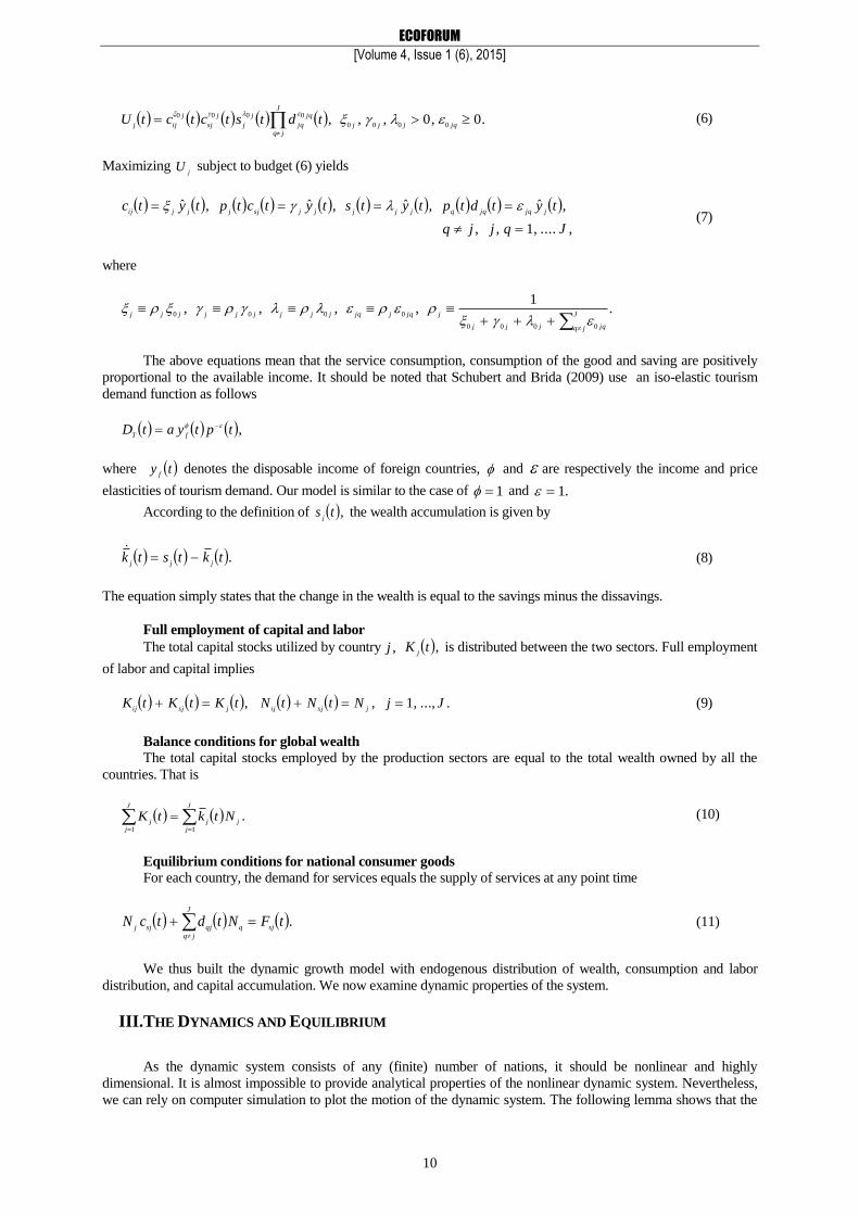
A rise in the LPE's population
It is well known that the relationship between population change and economic development is both
empirically and theoretically ambiguous. Some theoretical models show situation-dependent interactions between
population and economic growth (e.g., Galor and Weil, 1999; Boucekkine, et al., 2002; Bretschger, 2013). There
are also mixed conclusions in empirical studies on the issue (e.g., Furuoka, 2009; Yao et al., 2013). Although this
study is not concerned with endogenous population dynamics, we will study effects of changes in the population
sizes. We now show how the global economy is affected when the LPE experiences the following population
growth: .1110:3
N We plot the effects in Figure 3. The population growth brings about increases in the GGP and
global wealth. The contribution to the growth of the GGP is mainly due to the growth of the LPE's GDP as the other
two countries' GDPs are slightly affected. The rise of the population causes the rate of interest to increase and the
wage rates of all the countries to fall. The net consequence of the rise of interest and fall in the wage rate makes the
household in the HPE to accumulate more wealth and consume more the two goods, and the net consequences of the
rise of interest and fall in the wage rates make the households both in the PE and the LPE to accumulate less wealth
and consume less the two goods. The expenditures on tourism in the two countries from the HPE's household are
increased, and the expenditures on tourism in the two countries from each of the two other countries' household are
reduced. The price of consumer goods in the LPE is reduced as a consequence of enlarged population, and the prices
in the other two economies are slightly affected. The LPE produces more the two goods and employs more the two
input factors.
20 40 60
0.8
0.95
1.1
0 20 40 60
26
10
0 20 40 60
1
4.5
8
0 20 40 60
39
15
0 20 40 60
39
15
0 20 40 60
39
15
20 40 601
2.5
4
0 20 40 600
2
4
20 40 601
3
5
20 40 600.005
0.005
0.015
20 40 600.1
0.2
0.5
0 20 40 60
0.20.50.8
0 20 40 60
0.20.50.8
20 40 60
0.20.50.8
0 20 40 60
0.20.50.8
20 40 60
0.06
0.03
0
Figure 3 – A country's population being increased
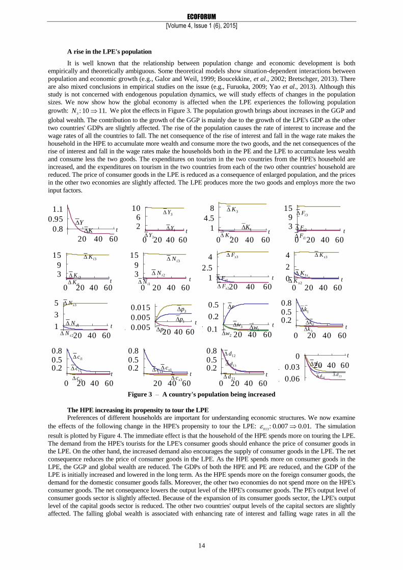
The HPE increasing its propensity to tour the LPE Preferences of different households are important for understanding economic structures. We now examine
the effects of the following change in the HPE's propensity to tour the LPE: .01.0007.0:013
The simulation
result is plotted by Figure 4. The immediate effect is that the household of the HPE spends more on touring the LPE.
The demand from the HPE's tourists for the LPE's consumer goods should enhance the price of consumer goods in
the LPE. On the other hand, the increased demand also encourages the supply of consumer goods in the LPE. The net
consequence reduces the price of consumer goods in the LPE. As the HPE spends more on consumer goods in the
LPE, the GGP and global wealth are reduced. The GDPs of both the HPE and PE are reduced, and the GDP of the
LPE is initially increased and lowered in the long term. As the HPE spends more on the foreign consumer goods, the
demand for the domestic consumer goods falls. Moreover, the other two economies do not spend more on the HPE's
consumer goods. The net consequence lowers the output level of the HPE's consumer goods. The PE's output level of
consumer goods sector is slightly affected. Because of the expansion of its consumer goods sector, the LPE's output
level of the capital goods sector is reduced. The other two countries' output levels of the capital sectors are slightly
affected. The falling global wealth is associated with enhancing rate of interest and falling wage rates in all the
t t t t
t t t t
t t t t
t t t
t
r
K
Y
3Y
1K
3K
2iF
1iF
1iK
3iK 3iN
2iN
1iN 1sF
2sF 2sK
sK1
1sN
2sN
3sK
3sN
3sc 2sc 1sc
1ic
3ic
2ic
2iK
3sF
32d
21d
13d
1p
2p
3p
1w 3w
1k
2k
31d
12d
23d
3iF
2K 1Y
2Y
3k 2w
ECOFORUM
[Volume 4, Issue 1 (6), 2015]
15
economies. The HPE's household accumulates less wealth. The wealth levels of the households in the PE and the
LPE are slightly affected. The consumption level of any of the two goods by any household is reduced. In fact,
empirical studies in the literature demonstrate an opposite relationship between a tourism boom and economic
development (for instance, Balaguer and Cantavella-Jorda, 2002; Dritsakis, 2004; Durbarry, 2004; Oh, 2005;
Kim et al. 2006). Harzri and Sgro (1995) show that an increase in the international tourism leads to a positive effect
on long-run economic growth of a small open economy. Our result shows that this conclusion is true in the short run,
but not necessarily true in the short term. We get this conclusion because our model explicitly shows transitional
processes of the economic dynamics and it deals with the world economy as an integrated whole. It should be also
noted that the study by Chao et al. (2006) shows that an expansion of tourism can result in capital decumulation in a
two-sector dynamic model with a capital-generating externality. Our simulation demonstrates the same conclusion in
the long term even without any externality.
20 40 60
0.2
0.5
1.2 20 40 600.4
0.1
0.6
20 40 601.5
0
1.5
20 40 60
16
8
0
20 40 60
16
8
0
20 40 60
16
8
0
20 40 600
8
16
20 40 600
8
16
20 40 60
0
8
16
20 40 600.01
0.02
0.05
20 40 600.5
0.5
1.5
20 40 60
2
1
0
20 40 60
2
1
020 40 60
2
1
0
0 20 40 60
0
20
40
20 40 60
0.2
0.1
0
Figure 4 – One country raising its propensity to tour another country
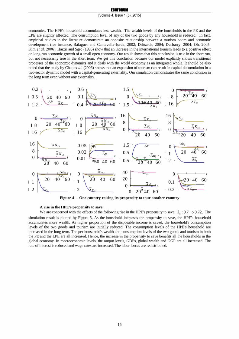
A rise in the HPE's propensity to save
We are concerned with the effects of the following rise in the HPE's propensity to save: .72.07.0:01
The
simulation result is plotted by Figure 5. As the household increases the propensity to save, the HPE's household
accumulates more wealth. As higher proportion of the disposable income is saved, the household's consumption
levels of the two goods and tourism are initially reduced. The consumption levels of the HPE's household are
increased in the long term. The per household's wealth and consumption levels of the two goods and tourism in both
the PE and the LPE are all increased. Hence, the increase in the propensity to save benefits all the households in the
global economy. In macroeconomic levels, the output levels, GDPs, global wealth and GGP are all increased. The
rate of interest is reduced and wage rates are increased. The labor forces are redistributed.
t t
t t
t t
t t
t
t t t
t t
t
t
r
K Y
3Y
1K
3K 2iF 1iF
1iK
3iK 3iN
2iN 1iN
1sF
2sF 2sK
sK1
1sN
2sN
3sK
3sN
3sc 2sc
1sc 1ic
3ic 2ic
2iK 3sF
32d 21d
13d
1p
2p
3p
1w
3w 1k
2k
31d
12d 23d
3iF
2K 1Y
2Y
3k
2w

ECOFORUM
[Volume 4, Issue 1 (6), 2015]
16
0 20 40 600
1
2
0 20 40 600
0.3
0.6
0 20 40 600
1
2
0 20 40 600
1
2
0 20 40 60
0
1
2
0 20 40 60
0
1
2
20 40 60
2.1
0.8
0.5
20 40 602
0
2
20 40 60
2
1
0
20 40 600.06
0.02
0.02
20 40 60
2.1
0.8
0.5
0 20 40 60
0.5
2
3.5
20 40 602
0.8
0.5
20 40 602
0.8
0.5
20 40 602
0.8
0.5
0 20 40 600
0.15
0.3
Figure 5 – A rise in the highly productive economy's propensity to save
A rise in the LPE's propensity to consume consumer goods We are concerned with the effects of the following rise in the LPE's propensity to consume consumer goods:
.1.008.0:03
The simulation result is plotted by Figure 6. The household in the LPE consumes more consume
goods, accumulates less wealth, consumes less consume goods, and tours less. The price of consumer goods in the
LPE falls and the prices in the other two economies are slightly affected. Consumption behavior of the households in
the HPE and the PE are slightly affected. The GGP and global wealth are reduced. As demonstrated in Figure 6, the
national economic structures also affected.
20 40 60
0.6
0.25
0.1
20 40 600.2
0
0.2
20 40 600.6
0
0.620 40 60
8
4
0
20 40 60
8
4
0
20 40 60
8
4
0
0 20 40 600
4
8
20 40 600
4
8
0 20 40 60
0
4
8
20 40 600.005
0.010.025
20 40 600.2
0.3
0.8
20 40 60
8
4
0
20 40 60
8
4
0
0 20 40 60
20
10
020 40 600.06
0.02
0.120 40 60
8
4
0
Figure 6 – A rise in an economy's propensity to consume consumer goods
t t t t
t t
t
t
t
t t
t
t t t
t
r
K Y
3Y
1K 3K
2iF 1iF
1iK 3iK
3iN 2iN
1iN 1sF
2sF 2sK
sK1
1sN
2sN
3sK
3sN
3sc 2sc 1sc
1ic 3ic
2ic
2iK 3sF
32d 21d
13d
1p
2p
3p
1w
3w 1k
2k
31d 12d 23d
3iF 2K 1Y
2Y
3k
2w
t t
t t
t t
t t
t
t t
t
t
t t
t
r
K Y
3Y
1K 3K
2iF 1iF
1iK
3iK 3iN
2iN
1iN
1sF
2sF 2sK sK1
1sN
2sN
3sK
3sN
3sc
2sc 1sc
1ic
3ic
2ic
2iK
3sF
32d 21d
13d
1p
2p
3p
1w
3w
1k
2k
31d
12d 23d
3iF 2K
1Y
2Y
3k 2w

ECOFORUM
[Volume 4, Issue 1 (6), 2015]
17
V.CONCLUDING REMARKS
This paper proposed an economic growth model to demonstrate dynamic interactions among economic
growth, economic structural change, international trade and tourist flows. It built a multi-country growth model with
endogenous wealth accumulation and tourism. The model is unique in this type of neoclassical growth models with
trade in that it introduces endogenous tourism within a general equilibrium framework. The model is built on
microeconomic foundations. It not only integrated the three well-known key models – the Solow growth model, the
Oniki-Uzawa trade model, and the Uzawa two-sector model - in growth theory and international growth economics,
but also introduced tourist flows between economies for any number of national economies. We demonstrated that
the motion of the J -country world economy can be described by J differential equations. We also simulated the
global economy with three countries, respectively called highly productive, productive, and lowly productive
economies. We showed that the world dynamics has a unique equilibrium. We carried out comparative dynamic
analysis with regard to one country's total productivity factor, the propensity to save, the propensity to tour other
countries, the population. It should also be remarked that our model can be extended and generalized in different
directions. For instance, it is significant to examine behavior of the dynamic system when the utility functions or/and
production functions are taken on other forms. The Solow model and Uzawa two-sector growth models are the two
key models in the neoclassical economic growth theory and the Oniki-Uzawa growth model is a main key model of
global economic dynamics with capital accumulation. These models have been generalized and extended in different
ways. We may extend our model on the basis of the contemporary literature of economics.
VI.APPENDIX: PROVING THE LEMMA
We now derive dynamic equations for global economic growth. From (2), we have
,sj
sjj
ij
ijj
j
k
jK
Nb
K
Na
w
rz
(A1)
where
.,sj
sj
j
ij
ij
jba
Insert ijijjj
KNaz // in ijijijkj
KFr / from (2)
.,...,1, Jjza
Azr
kj
ij
jij
j
ijij
j
(A2)
From (A2) we get
.,...,2,
/1
1Jj
A
razz
ij
ijij
kj
jj
(A3)
From (A1) and (A2), we have
.1
j
kj
jz
rzw
(A4)
From sjsjjj
KNbz / and (1), we have
.1 sj
jsjsj
kj
sj
j
jzA
rbzp
(A5)
From (11) and (7) we have

ECOFORUM
[Volume 4, Issue 1 (6), 2015]
18
.ˆˆsjj
J
jq
qqqjjjjFpNyNy
(A6)
Insert (1) in (A6)
.ˆˆsj
sjjJ
jq
qqqjjjj
NwNyNy
(A7)
By (3) we have
.1,ˆ1 jjjj
wkrkzy (A8)
Substituting (A8) into (A7) yields
,,1 j
J
jq
qqqjjjjjjsjRkNkNRkzN
(A9)
where
.,1
11
J
jq
qqjq
j
js
jjsjjsj
j
jNw
wNzR
w
rzR
From jsjij
NNN and (A9), we solve
.,1 sjjjij
NNkzN (A10)
With (A10) and (A11) we determine the labor distribution as functions of 1
z and .q
k From (A1) and
(A10) we have
.,,,11
j
sjj
jsj
j
ijj
jijz
NbkzK
z
NakzK (A11)
From (9) and (10), we have
.11
j
J
j
j
J
j
sjijNkKK
(A12)
Inserting (A12) in (A11) implies
.111
j
J
j
j
J
j
sjj
J
j j
jjNkNz
z
Na
(A13)
where ./jjjj
zabz Insert (A9) in (A13)
.110
1
11111NkRRzkNkRzN
J
j
jj
J
jq
qqqj
(A14)
where
.,2112
10
J
j
jjjjj
J
j
jj
J
j j
jj
j
J
j
jjkRzNRz
z
NaNkkzR
ECOFORUM
[Volume 4, Issue 1 (6), 2015]
19
where .,...,2 Jj
kkk Solve (A14) with respect to 1
k
.1
1
,
1
1
2
1111
2 1,
11
2
10
11
NRzRzRzkNRzkNR
kzk
J
j
jjj
J
j
jj
J
jq
qqqj
J
q
qqq
j
(A15)
Substitute jj
ys ˆ and jj
wkr into (8)
,1,111101
wrkzkj
(A16)
.,...,2,1,1
Jjkwkrkzkjjjjjjjj
(A17)
Taking derivatives of equation (A15) with respect to t yields
,2
1
1
1
J
j j
jk
zz
k (A18)
where we use (A17). Insert (A18) in (A16)
.,
1
12
0111
zkkzz
J
j j
jj (A19)
Following the procedure in the lemma we describe the dynamics of the economic system.
VII.ACKNOWLEDGMENT
The author is grateful to the effective co-operation of Editor Alexandru Mircea Nedelea. The author is also
grateful for the financial support from the Grants-in-Aid for Scientific Research (C), Project No. 25380246,
Japan Society for the Promotion of Science.
VIII.REFERENCES
Almazan, A., DeMotta, A., Titman, S. (2007) Firm location and the creation and utilization of human capital, Review of Economic
Studies, 74, pp. 1305–27.
Balaguer, L., Cantavella-Jorda, M. (2002) Tourism as a long-run economic growth factor: The Spanish case, Applied Economics, 34, pp. 877-84.
Benhabib, J., Meng, Q.L, Nishimura, K. (2000) Indeterminacy under constant returns to scale in multisector economy, Econometrica, 68, pp.
1541-48. Blake, A., Sinclair, M.T., Campos, J.A. (2006) Tourism productivity – Evidence from the United Kingdom, Annals of Tourism Research, 33,
pp. 1099-120.
Boucekkine, R., de la Croix, D., Licandro, O. (2002) Vintage human capital. demographic trends, and endogenous growth, Journal of Economic Growth, 104, pp. 340-75.
Brecher, R.A., Chen, Z.Q., Choudhri, E.U. (2002) Absolute and comparative advantage, reconsidered: The pattern of international trade with
optimal saving, Review of International Economics, 10, pp. 645-56. Bretschger, L. (2013) Population growth and natural-resource scarcity: Long-run development under seemingful unfavorable conditions, The
Scandinavian Journal of Economics, 115, pp. 722-55.
Burmeister, E, Dobell, A.R. (1970) Mathematical Theories of Economic Growth, Collier Macmillan Publishers, London. Busse, M., Hefeker, C. (2007) Political risk, institutions and foreign direct investment, European Journal of Political Economy, 23, pp.
397–415.
Chao, C.C., Hazari, B.R., Laffargue, Y.P., Yu, E. S.H. (2006) Tourism, dutch disease and welfare in an open dynamic economy, Japanese Economic Review, 57, pp. 501-15.
Chao, C.C., Hazari, B.R., Laffargue, Y.P., Yu, E. S.H. (2009) A dynamic model of tourism, employment, and welfare: The case of Hong Kong.
Pacific Economic Review, 14, pp. 232-45. Colombo, L., Dawid, H. (2014) Strategic location choice under dynamic oligopolistic competition and spillovers, Journal of Economic
Dynamics & Control (forthcoming).
Copeland, B. R. (1991) Tourism, welfare and de-industrialization in a small open economy, Economica, 58, pp. 515-29. Corden, W.M., Neary, J.P. (1982) Booming sector and de-industrialization in a small open economy, Economic Journal, 92, pp. 825-48.
Cremers, E.T. (2006) Dynamic efficiency in the two-sector overlapping generalizations model, Journal of Economic Dynamics & Control,
30, pp. 1915-36.
ECOFORUM
[Volume 4, Issue 1 (6), 2015]
20
De Beule, F., Duanmu, J.L. (2012) Locational determinants of internationalization: A firm-level analysis of Chinese and Indian
acquisitions, European Management Journal, 30, pp. 264–77.
Diamond, P.A. (1965) Disembodied technical change in a two-sector model, Review of Economic Studies, 32, pp. 161-68. Dritsakis, N. (2004) Tourism as a long-run economic growth factor: An empirical investigation for Greece using causality analysis, Tourism
Economics, 10, pp. 305-16.
Drubarry, R. (2004) Tourism and economic growth: The case of Mauritius, Tourism Economics, 10, pp. 389-401. Drugeon, J.P., Venditti, A. (2001) Intersectoral external effects, multiplicities & indeterminacies, Journal of Economic Dynamics & Control,
25, pp. 765-87.
Dwyer, L., Forsyth, P., Spurr, R. (2004) Evaluating tourism’s economic effects: New and old approaches, Tourism Management, 25, pp. 307-17.
Frenkel, J.A., Razin, A. (1987) Fiscal Policy and the World Economy, MIT Press, MA., Cambridge.
Furuoka, F. (2009) Population growth and economic development: New empirical evidence from Thailand, Economics Bulletin, 29, pp. 1-14.
Galor, O. (1992) Two-sector Overlapping-generations Model: A Global Characterization of the Dynamical System. Econometrica 60,
1351-86. Galor, O., Weil, D. (1999) From Malthusian stagnation to modern growth, American Economic Review, 89, pp. 150-54.
Gaŕin-Mũnos, T. (2007) German demand for tourism in Spain, Tourism Management, 28, pp. 12-22.
Hazari, B.R., Lin, J.J. (2011) Tourism, terms of trade and welfare to the poor, Theoretical Economics Letters, 1, pp. 28-32. Hazari, B.R., Sgro, P.M. (1995) Tourism and growth in a dynamic model of trade, Journal of International Trade and Economic
Development, 4, pp. 243-52.
Hazari, B.R., Sgro, P.M. (2004) Tourism, Trade and National Welfare, Elsevier, Amsterdam.
Henisz, W.J. (2000) The institutional environment for multinational investment, Journal of Law, Economics and Organization, 6, pp.
334–64.
Ikeda, S., Ono, Y. (1992) Macroeconomic dynamics in a multi-country economy - A dynamic optimization approach. International Economic Review, 33, pp. 629-44.
Kim, H.J., Chen, M.H., Jang, S. (2006) Tourism expansion and economic development: the case of Taiwan, Tourism Management, 27, pp.
925-33. Lanza, A., Temple, P., and Urga, G. (2003) The Implications of Tourism Specialisation in the Long Run: An Econometric Analysis for 13
OECD Economies. Tourism Management 24, 315-21.
Lee, C. C. and Chang, C. P. (2008) Tourism Development and Economic Growth: A Closer Look at Panels. Tourism Management 29, 180-192.
Lee, J.Y., Mansfield, E. (1996) Intellectual property protection and us foreign direct investment, Review of Economics and Statistics,
78, pp. 181–86. Li, J.L. Lin S.L. (2008) Existence and uniqueness of steady-state equilibrium in a two-sector overlapping generations model, Journal of
Economic Theory, 141, pp. 255-75.
Mino, K. (1996) Analysis of a two-sector model of endogenous growth with capital income taxation, International Economic Review, 37, pp. 227-51.
Nishimura, K., Shimomura, K. (2002) Trade and indeterminacy in a dynamic general equilibrium model. Journal of Economic Theory
105, pp. 244-60. Oh, C.O. (2005) The contribution of tourism development to economic growth in the Korean economy, Tourism Management, 26, pp. 39-44.
Oniki, H., Uzawa, H. (1965) Patterns of trade and investment in a dynamic model of international trade, Review of Economic Studies, 32, pp. 15-38.
Ortigueira, S., Santos, M.S. (2002) Equilibrium dynamics in a two-sector model with taxes, Journal of Economic Theory, 105, pp. 99-119.
Schubert, S. F., Brida, J.G. (2009) A dynamic model of economic growth in a small tourism driven economy, Munich Personal RePEc Archive. Schubert, S., Brida, J., Risso, A. (2011) The impacts of international tourism demand on economic growth of small economies dependent
on tourism, Tourism Management, 32, pp. 377-85
Seentanah, B. (2011) Assessing the dynamic economic impact of tourism for island economies, Annals of Tourism Research, 38, pp. 291- 308
Sinclair, M. (2002) Tourism and economic development: A survey, The Journal of Development Studies, 34, pp. 1-51.
Sinclair, M.T., Stabler, M. (1997) The Economics of Tourism, Routledge, London. Solow, R. (1956) A contribution to the theory of growth, Quarterly Journal of Economics, 70, pp. 65-94.
Sorger, G. (2002) On the multi-country version of the Solow-Swan model, The Japanese Economic Review, 54, pp. 146-64.
Stiglitz, J.E. (1967) A two sector two class model of economic growth, Review of Economic Studies, 34, pp. 227-38. Stockman, D.R. (2009) Chaos and sector-specific externalities, Journal of Economic Dynamics and Control, 33, pp. 2030-46.
Sun, Y. (2014) A framework to account for the tourism carbon footprint at island destinations, Tourism Management, 45, pp. 16-27.
Syriopoulos, T.C. (1995) A dynamic model of demand for Mediterranean tourism, International Review of Applied Economics, 9, pp. 318-36.
Uzawa, H. (1961) On a two-sector model of economic growth, Review of Economic Studies, 29, pp. 47-70.
Uzawa, H. (1963) On a two-sector model of economic growth I, Review of Economic Studies, 30, pp. 105-18. Yao, W.J., Kinugasa, T., Hamori, S. (2013) An empirical analysis of the relationship between economic development and population
growth in China. Applied Economics, 45, pp. 4651-61.
Zhang, W.B. (1993) Woman’s labor participation and economic growth - creativity, knowledge utilization and family preference, Economics Letters, 42, pp. 105-10.
Zhang, W.B. (2012) Global economic growth, trade patterns and non-tradable services, Global Business & Economics Anthology, 1,
pp. 296-306. Zhang, W.B. (2012) Tourism and economic structure in a small-open growth model, Journal of Environmental Management and
Tourism, 2, pp. 76-92.
Zeng, D.Z., Zhu, X.W. (2011) Tourism and industrial agglomeration, The Japanese Economic Review, 62, pp. 537-61.