total material requirement of the european...
TRANSCRIPT

Technical report No 56
Total material requirement of the European Union
Technical part
Prepared by: Stefan Bringezu
Helmut Schütz (Wuppertal Institute)
Project Manager: Peter Bosch
European Environment Agency

2
Cover design: Rolf Kuchling, EEA This report describes the methodology used to calculate the indicators in Chapter 16 (‘Total material requirements’) of Environmental signals 2000. A more extensive description of total material requirements and more results can be found in EEA technical report No 55 Total material requirement of the European Union. Legal notice Neither the European Environment Agency nor any person or company acting on behalf of the Agency is responsible for the use that may be made of the information contained in this report. A great deal of additional information on the European Union is available on the Internet. It can be accessed through the Europa server (http://europa.eu.int) © EEA, Copenhagen, 2001 Reproduction is authorised provided the source is acknowledged Printed in Denmark Printed on recycled and chlorine-free bleached paper
European Environment Agency Kongens Nytorv 6 DK-1050 Copenhagen K Tel: (45) 33 36 71 00 Fax: (45) 33 36 71 99 E-mail: [email protected] Internet: http://www.eea.eu.int

3
Contents
1. Introduction and overview ..........................................................5
2. Domestic material flows ..............................................................9
2.1. Agriculture ...................................................................................................... 9
2.2. Excavation..................................................................................................... 12
2.3. Forestry, fishing, hunting............................................................................... 13
2.4. Fossil energy ................................................................................................. 14
2.5. Minerals......................................................................................................... 17
2.6. Ores .............................................................................................................. 23
3. Foreign material flows...............................................................28
3.1. Agricultural raw materials.............................................................................. 29
3.2. Forestry raw materials ................................................................................... 31
3.3. Animals as raw materials and products.......................................................... 31
3.4. Agricultural plant products............................................................................ 31
3.5. Agricultural animal products.......................................................................... 32
3.6. Forestry semi-manufactured products ........................................................... 34
3.7. Forestry finished products............................................................................. 34
3.8. Biotic products .............................................................................................. 34
3.9. Fossil energy carriers, raw materials.............................................................. 35
3.10. Metals, raw materials .................................................................................... 36
3.11. Minerals, raw materials.................................................................................. 43
3.12. Fossils, semi-manufactured products ............................................................. 44
3.13. Metals, semi-manufactured products............................................................. 45
3.14. Minerals, semi-manufactured products .......................................................... 48
3.15. Metals, finished products .............................................................................. 48
3.16. Minerals, finished products............................................................................ 49
3.17. Abiotic products............................................................................................ 50
3.18. Other products.............................................................................................. 50

4
3.19. Summary of imports ...................................................................................... 51
4. General data .............................................................................56
5. TMR data summary ...................................................................57
6. References ................................................................................59

5
1. Introduction and overview
The concept of ‘total material requirement’ (TMR) was originally developed at the Wuppertal Institute under the label ‘total material input’ (TMI) (for a recent overview, see Bringezu, 2000). The TMR of national economies comprises two major components: domestic material flows and foreign material flows (Adriaanse et al., 1997, 1998). These are further subdivided into direct material inputs (DMI) and hidden material flows which were originally called ‘ecological rucksacks’ in the MIPS-concept (Schmidt-Bleek et al., 1998). TMR and its sub-components are commonly set into relation with GDP and population size to obtain the material productivity or material intensity of GDP of the economy, and the total material flows per capita. Both are aggregate measures for the total environmental impact of national or regional economies. The basic structure of TMR is reflected in its first order accounting components shown in Figure 1. These are: domestic (material flows); foreign (material flows); general (socio-economic data); summary (for TMR accounting and analysis). Figure 1 further provides an overview of the files (light shading) and workbooks or worksheets (without shading) contrasted with structure data for TMR accounting of EU-15. Transfer of data by automatic links from worksheets to the ‘TMR data summary’ workbook are marked with heavy shading. This overview will be the reference for the further description of the methodology of TMR in the following chapters. It shall also provide easy access to those who wish to perform similar studies or use the data of EU-15 for further studies and applications. The ‘territory’ of EU-15 was established with the accession of Austria, Finland and Sweden in 1995.Until then, the European Community had gradually developed from its beginnings in 1952 (Table 1). Monetary union is still incomplete in the year 2000 and 12 candidate countries are currently negotiating for accession. Table 1: Member States of the European Union Year of accession Member of monetary union Belgium 1952/58 * X France 1952/58 * X Germany 1952/58 * X Italy 1952/58 * X Luxembourg 1952/58 * X Netherlands 1952/58 * X Denmark 1973 ** Ireland 1973 X United Kingdom 1973 Greece 1981 *** Portugal 1986 X Spain 1986 X Austria 1995 X Finland 1995 X Sweden 1995
* 1952: European Community for Coal and Steel
1958: European Economic Community
** Denmark will decide on application for membership by public vote in September 2000, Sweden and the UK will also hold public votes.
*** Greece has officially applied for membership (as of March 2000)
Candidate countries (12) are: Estonia, Latvia, Lithuania, Poland, Czech Republic, Slovakia, Hungary, Slovenia, Romania, Bulgaria, Cyprus, Malta.

6
Domestic Agriculture 00-FAO Data Original Foreign 00-Imports-General
00-General 01-Imports-AgricultureRaw01-Cereals 02-Imports-ForestryRaw02-Roots and tubers 03-Imports-AnimalsRaw+Products03-Pulses 04-Imports-AgricultPlantProduct04-Oilcrops 05-Imports-AgricultAnimalProduc05-Vegetables+melons 06-Imports-ForestrySemi06-Fruit excl. melons 07-Imports-ForestryFinished07-Treenuts 08-Imports-BioticProducts08-Fibre crops 09-Imports-FossilsRaw09-Other cops 10-Imports-MetalsRaw10-AgriHarvestStatisticsSummary TMR Data Summary 11-Imports-MineralsRaw11-Other Harvest TMR Data Summary 12-Imports-FossilsSemi12-Other Fodder Inputs TMR Data Summary 13-Imports-MetalsSemi13-AgricultureTotalInputSummary 14-Imports-MineralsSemi14-Erosion TMR Data Summary 15-Imports-MetalsFinished
Excavation 01-ExcavationDomestic TMR Data Summary 16-Imports-MineralsFinishedForestry, Fishing, Hunting 01-Roundwood TMR Data Summary 17-Imports-AbioticProducts
02-Fish catch TMR Data Summary 18-Imports-OtherProducts03-Hunting TMR Data Summary 19-EU12-Imports889404-Aquatic mammals(numbers) Summary SUMMARY Imports05-AquaticData-FAO TMR Data Summary
FossilEnergy 01-EnergyHardCoalDomestic02-EnergyLigniteDomestic03-EnergyCrudeOilDomestic General GDP85-97 TMR Data Summary04-EnergyNaturalGasDomestic Population85-98 TMR Data Summary05-EnergyCrudeOilGasDomestic06-EnergyPeatFuelDomestic07-EnergyPeatAgricultDomestic Summary TMR Data Summary08-EnergyOilshaleDomestic09-EnergySummaryDomestic TMR Data Summary

7
MineralsDomestic 00-Commodities/Sources01-MineralsA,C,E,Domestic02-MineralsB,Domestic03-MineralsD,Domestic04-MineralsPhosphateDomestic05-MineralsPotashDomestic06-MineralsSaltsDomestic07-MineralsBarytesDomestic08-MineralsFluorsparDomestic09-MineralsAsbestosDomestic10-MineralsMagnesiteDomestic11-MineralsBoratesDomestic12-MineralsArsenicDomestic13-MineralsAbrasivesDomestic14-MineralsGraphiteDomestic15-MineralsMicaDomestic16-MineralsOtherDomestic17-MineralsSummaryDomestic TMR Data Summary
OresDomestic 01-OresIronDomestic02-OresCopperDomestic03-OresZincDomestic04-OresLeadDomestic05-OresBauxiteDomestic06-OresTinDomestic07-OresTungstenDomestic08-OresVanadiumDomestic09-OresManganeseDomestic10-OresChromiumDomestic11-OresNickelDomestic12-OresTitaniumDomestic13-OresSilverDomestic14-OresGoldDomestic15-OresTantalumNiobiumDomestic16-OresAntimonyDomestic17-OresCobaltDomestic18-OresMercuryDomestic19-OresUraniumDomestic20-OresPyritePyrrhotiteDomestic21-OresSummaryDomestic TMR Data Summary
File Worksheets/Workbooks Automatic links to TMR Data Summary Figure 1: Basic structure of data files and worksheets for the accounting of TMR in the EU.

8
The step-by-step development of the European Union is reflected by the data availability for TMR accounting. A consistent time series of TMR for the EU-15 could be established for 1995–97. Before that, a time series was worked out for EU-12 from 1988 to 1994. It has to be noted, however, that this series was affected by the German reunification. Data for the former GDR were integrated into foreign trade statistics of Eurostat since 1991. Consequently, TMR of EU-12 from 1988 to 1990 is exclusive of the former GDR, but data from 1991 to 1994 include the ‘five new Länder’ evolving from it as part of the reunited Germany. The corresponding changes in population, GDP and GDP per capita are shown in Table 2. Table 2: Population, GDP and GDP per capita of EU-12 and EU-15 from 1988 to 1997 Year Population * GDP ** GDP per
capita *** Population #
GDP #
GDP per capita #
EU-12 excl. former GDR 1988 323 425 3 700 11 440 100 100 100 1989 324 747 3 827 11 785 100 103 103 1990 326 646 3 940 12 062 101 106 105
EU-12 incl. former GDR 1991 344 251 4 221 12 262 106 114 107 1992 345 832 4 270 12 347 107 115 108 1993 347 391 4 267 12 284 107 115 107 1994 348 593 4 482 12 856 108 121 112
EU-15 1995 371 588 5 018 13 504 115 136 118 1996 372 850 5 285 14 175 115 143 124 1997 373 890 5 615 15 019 116 152 131 * 1 000 persons
** Billion ECU at 1985 constant prices
*** ECU per capita
# Indexed values with 1988 = 100

9
2. Domestic material flows
The following chapters will give descriptions of data and methods for the step-by-step accounting of domestic material flows of EU-15 as encompassed by the left hand side of Figure 1. Its major components are organised in the following sections (in alphabetical order): agriculture; excavation; forestry, fishing, hunting; fossil energy; minerals, domestic; ores, domestic.
2.1. Agriculture
For easy access to data, the service on the FAO homepage (http://apps.fao.org) was used for downloading data on harvested biomass and land use in agriculture, roundwood production in forestry, and the amount of biomass from fishing. The original FAO data were kept in the file 00 ‘FAO data/original’. File 00 ‘General’ contains two worksheets: agriareaEU158597; EU-15 All FAO categories. Worksheet ‘agriareaEU158597’ contains land-use data in hectare by Member States for arable land, permanent crops, and permanent pastures, the three main categories making up the total agricultural area. It is the basis for (a) the accounting of the input of biomass which is not given by harvest statistics, and (b) the estimation of the amount of erosion using intensity figures in tonnes soil eroded per hectare land. Worksheet ‘EU-15 all FAO categories’ lists all the categories of agricultural biomass available from the FAO database (http://apps.fao.org) and groups them under the main headings as shown in Table 3. The respective data are contained in worksheets 01 to 09 as shown in Figure 1. In each worksheet, a summary table is made with respect to the distribution among the Member States, and another summary table is made with respect to the aggregate of the nine main groups for EU-12 and EU-15. These summary tables are marked (light yellow for Member countries and light blue by main material groups) for easy identification within the worksheet (a procedure used for all the data collected for TMR in EU-15). They are transferred to the worksheet 10 ‘Agri/harvest/statistics/summary’ by automatic link to obtain the total of biomass material flows reported by FAO agricultural harvest statistics. The resulting summary tables in this worksheet are transferred, again by automatic link, to the final data compilation in workbook ‘TMR data summary’. In addition to biomass reported to be harvested by agricultural statistics, there are biomass inputs which are not reported there but nevertheless used (worksheet 11 ‘Other harvest’):

10
sugar beet leaves; fodder beet leaves; straw input; catch crops. Sugar beet leaves used as feed from domestic production for agricultural animals are reported in statistics of the German Ministry of Nutrition, Agriculture and Forestry, the ratio of leaves to beets being about 0.67. This multiplier was used to account for the input of sugar beet leaves in the EU-15 based on the data for sugar beet harvested in Member States. The same procedure was done for fodder beet leaves, the ratio of leaves to beets being about 0.23 in that case. It was also done for straw from grains production using a ratio of 0.46 of straw to grains (on the assumption that 50 % of total straw production was used as an input for further processing). Catch crops are also reported under foodstuffs from domestic production for agricultural animals in statistics of the German Ministry of Nutrition, Agriculture and Forestry. No specific information was available for other EU-15 Member States, so only the German data were used. The resulting summary tables in this worksheet are transferred, again by automatic link, to the final data compilation in workbook ‘TMR data summary’.
Agricultural biomass represented in harvest statistics mostly refer to crops cultivated on arable land and permanent crops. The third main category of agricultural land use, permanent pastures, may either be harvested to produce animal foodstuff or may be used for grazing of animals. The first use is represented in statistics. The latter use, which may be characterised as harvested by animals, is a used material input flow just as harvested biomass by machinery is, but is not represented in harvest statistics. To account for this input, the following procedure was performed (worksheet 12 ‘Other fodder inputs’):
First, all the biomass categories from harvest statistics which were attributable to permanent pastures were filtered out. These were: alfalfa for forage and silage, clover for forage and silage, forage products nes (not elsewhere specified), grasses nes for forage and silage, and rye grass for forage and silage. The total land use of these categories was subtracted from the total area of permanent pastures.
Second, the remaining area of permanent pastures was the basis for an estimate of the related input of green biomass by animals’ grazing. Consequently, yield coefficients had to be found in order to account for the input of biomass by grazing in tonnes where direct data were not available.
Third, direct data for the input of biomass by grazing was derived from German foodstuffs statistics of the Ministry of Nutrition, Agriculture and Forestry. They corresponded to yields in between about 12 to 15 tonnes per hectare of permanent pasture. For Austria, the total amount of foodstuff by grazing was available from the database of the Institute for Interdisciplinary Research and Continuing Education in Vienna (IFF), and these figures were directly used.

11
Table 3: Main groups and categories of biomass from agricultural harvest
Source: FAO database (http://apps.fao.org), own compilation. Finally, for the remaining territory of EU-13 (EU-15 excluding Austria and
Germany), the German yields were multiplied by the area of non-harvested permanent pastures. The result was an estimate for the input of fodder biomass by grazing of agricultural animals.
The resulting summary tables in this worksheet are transferred, again by automatic link, to the final data compilation in workbook ‘TMR data summary’. The total domestic direct material input by agriculture is summarised in worksheet 13 ‘Agriculture/total input/summary’, comprising the data from worksheets 10, 11 and 12. Erosion of soil from arable land was estimated for the following categories of land use (worksheet 14‘Erosion’): roots and tubers; sugar beets; fodder beets; maize for fodder; arable land, excluding maize, roots and tubers, sugar and fodder beets. Erosion rates shown in Table 4 were used to account for estimates of soil erosion from arable land (from the database of the Wuppertal Institute). Data for soil erosion in Finland were taken directly from the database of the Thule Institute at the University of Oulu, Finland (Juutinen and Mäenpää, 1999). Data for soil erosion in the Netherlands were taken directly from the resource flows study (Adriaanse et al., 1997). The resulting summary tables in this worksheet are transferred, again by automatic link, to the final data compilation in workbook ‘TMR data summary’.
01 02 03 04 05 06 07 08 09Cereals Roots and Tubers Pulses Oilcrops Vegetables & melons Fruit excluding melons Treenuts Fibre crops Other cropsBarley Potatoes Beans, dry Groundnuts in shell Artichokes Apples Almonds Cotton lint Alfalfa for forage+silagBuckwheat Roots and tubers nes Broad beans, dry Hempseed Asparagus Apricots Chestnuts Flax fibre and tow Anise, badian, fennelCanary seed Sweet potatoes Chick-peas Linseed Beans, green Avocados Hazelnuts (filberts) Hemp fibre and tow Beets for fodderCereals nes Yams Lentils Melonseed Broad beans, green Bananas Nuts Nes Cabbage for fodderMaize Lupins Mustard seed Cabbages Berries nes Pistachios Carrots for fodderMillet Peas, dry Oilseeds Nes Cantaloupes & oth melons Blueberries Walnuts Chicory rootsMixed grain Pulses nes Olives Carrots Carobs Clover for forage + silageOats Vetches Poppy seed Cauliflower Cherries CottonseedRice, paddy Rapeseed Chillies & peppers, green Citrus fruit nes Forage products nesRye Safflower seed Cucumbers and gherkins Currants Grasses nes, forage + silageSorghum Seed cotton Eggplants Dates Hay (unspecified)Triticale Sesame seed Garlic Figs HopsWheat Soya beans Green corn (maize) Fruit fresh nes Leguminous nes,, for .+ sil.
Sunflower seed Leeks and oth.alliac.veg Fruit tropical fresh nes Maize for forage + silageLettuce Gooseberries PeppermintMushrooms Grapefruit and pomelos Pimento, allspiceOnions + shallots, green Grapes Pumpkins for fodderOnions, dry Kiwi fruit Pyrethrum, dried flowersPeas, green Lemons and limes Rye grass, forage + silagePumpkins, squash, gourds Oranges Sorghum for forage + silageSpinach Peaches and nectarines Spices nesString beans Pears Sugar beetsTomatoes Persimmons Sugar caneVegetables fresh nes Pineapples Swedes for fodderWatermelons Plums Tea
Quinces Tobacco leavesRaspberries Turnips for fodderSour cherries Vegetables + roots, fodderStone fruit nes, freshStrawberriesTang.mand.clementines, satsumas
Nes = Not elsewhere specified

12
Table 4: Erosion rates (tonnes per ha) for estimates of soil erosion from arable land Roots and
tubers Sugar beets Fodder beets Maize for
fodder Other arable land
EU-12 18 18 18 55 15
EU-15 17 17 17 51 14
Belgium 13 13 13 38 10
Denmark 6 6 6 19 5
Germany 10 10 10 30 8
Greece 31 31 31 94 25
Spain 31 31 31 94 25
France 13 13 13 38 10
Ireland 6 6 6 19 5
Italy 19 19 19 56 15
Austria 19 19 19 56 15
Portugal 31 31 31 94 25
Sweden 6 6 6 19 5
United Kingdom 11 11 11 34 9
2.2. Excavation
Data for this type of hidden flows comprise excavations for infrastructures and dredging for navigation purposes. They are organised in a single worksheet called 01 ‘Excavation/domestic’. In the follow-up to the resource flows study (Adriaanse et al., 1997), these material flows have recently been accounted for the United States, Japan, the Netherlands, Austria and Germany in time series. In addition, these data are available for Finland in time series (database of the Thule Institute at University of Oulu, Finland, Juutinen and Mäenpää, 1999). Single data for soil excavation were also reported for Belgium in 1992 and for the UK in 1993.
To obtain basic coefficients for estimates of excavation flows in other EU-15 Member States, these given values were divided by gross value added for constructions (the latter from Eurostat statistics). Resulting coefficients were expressed in the first case as tonnes soil excavated per million ECU gross value added (Table 5). The weighted average for Germany, Netherlands, Austria and Finland was used to estimate soil excavation in tonnes for the remaining Member States of EU-15 except Belgium and the UK. Coefficients for 1996 were used to account for soil excavation in 1997 (except Finland).

13
Table 5: Soil excavated (tonnes) per million ECU gross value added for constructions 1985 1986 1987 1988 1989 1990 1991 1992 1993 1994 1995 1996 1997
Belgium 106
Denmark
Germany (West) 3 227 3 349 3 348 3 396 3 433 3 345
Germany 3 823 3 337 3 416 3 613 2 991 3 035
Greece
Spain
France
Ireland
Italy
Luxembourg
Netherlands 3 618 3 869 4 015 3 061 3 065 2 664 2 650 2 789 2 618 2 538 2 363 2 373
Austria 5 209 5 191 5 117 4 993 4 810 4 605 4 305 4 142 4 007 3 779 3 665 3 633
Portugal
Finland 8 164 8 359 8 099 7 456 6 505 6 983 8 098 11 272 12 318 10 337 6 870 6 199 5 384
Sweden
United Kingdom 923
Weighted average: D,NL,A, FIN
3 863 4 000 4 019 3 849 3 807 3 707 4 001 3 669 3 665 3 756 3 148 3 163
A similar procedure as for the estimation of soil excavation was performed for dredging. In that case, coefficients obtained for the Netherlands were considered to reflect a specific single situation. To obtain estimates for the EU, the German coefficient for 1990 was used (Table 6). Coefficients for 1996 were used to account for dredging in 1997. Table 6: Dredged material (tonnes) per million ECU gross value added for constructions 1985 1986 1987 1988 1989 1990 1991 1992 1993 1994 1995 1996 1997 EU-12 EU-15 Belgium Denmark Germany (West) 665 Germany Greece Spain France Ireland Italy Luxembourg Netherlands 9 483 7 970 7 461 6 418 5 981 6 248 5 847 5 468 5 043 4 468 3 806 3 454 Austria Portugal Finland Sweden United Kingdom The resulting summary tables in this worksheet are transferred, again by automatic link, to the final data compilation in workbook ‘TMR data summary’.
2.3. Forestry, fishing, hunting
The data for this group of domestic material inputs were organised in the following way:

14
01: Roundwood; 02: Fish catch; 03: Hunting; 04: Aquatic mammals (numbers only, not tonnes); 05: Aquatic data FAO. So, only worksheets 01 to 03 contained data in tonnes for transfer to the final data compilation in workbook ‘TMR data summary’ by automatic link. Worksheet 04 contains FAO data on the number of aquatic mammals caught (eared, hair seals, walruses; blue-whales, fin-whales; sperm-whales, pilot-whales) but these are so scattered that they could not even be used to produce an overview for a single year. File 05 , ‘Aquatic data/FAO’, contains the FAO data documented in worksheets 01 to 04. Data for raw material input from forestry (worksheet 01 ‘Roundwood’) were downloaded from the FAO web site (http://apps.fao.org). The total volume of roundwood was classified in the following way: coniferous roundwood; non-coniferous roundwood; wood for charcoal. Data are reported in cubic metres of roundwood excluding barks. They were converted into tonnes using the following coefficients, derived from German statistics: coniferous roundwood (0.75 tonnes per m3), non-coniferous roundwood (0.85 tonnes per m3), and wood for charcoal (0.8 tonnes per m3). Besides data for Germany (from the database of the Wuppertal Institute), original data for total roundwood input were also available in tonnes for Austria (database of the Institute for Interdisciplinary Research and Continuing Education in Vienna — IFF) and for Finland (database of the Thule Institute at University of Oulu, Finland; Juutinen and Mäenpää, 1999). These were directly inserted into the database without converting the FAO data from m3 to tonnes. Data for raw material input from fishing (worksheet 02 ‘Fish catch’) were also downloaded from the FAO web site (http://apps.fao.org). Total fish catch and its sub-category total marine fish catch were differentiated, the difference being attributed to the category ‘other aquatic catch excluding mammals’. For Finland, data on wild fish catch were taken from the database of the Thule Institute at the University of Oulu, Finland (Juutinen and Mäenpää, 1999), instead of the FAO data. The hidden flows of fish catch were estimated according to a study of Greenpeace (Frankfurter Rundschau of 6 November 1999) after which 25 % of the catch is being discarded on board (by-catch). Data for raw material input from hunting (worksheet 03 ‘Hunting’) have so far been quantified for Germany (database of the Wuppertal Institute; see also Schütz and Bringezu, 1998). No other source could be found reporting on this type of input in other EU Member States.
2.4. Fossil energy
The material inputs of this group of fossil energy carriers comprise all inputs whether they are used for energetic conversion or not. While the non-energetic use of peat for agriculture is obvious, it would be hard to identify the non-energetic use of coal, crude petroleum or natural gas. The following sub-categories are counted in separate worksheets named:

15
01: Energy/hard coal/domestic; 02: Energy/lignite/domestic; 03: Energy/crude oil/domestic; 04: Energy/natural gas/domestic; 05: Energy/crude oil/gas/domestic; 06: Energy/peat/fuel/domestic; 07: Energy/peat/agricult./domestic; 08: Energy/oil shale/domestic. Worksheet 09 ‘Energy/summary/domestic’ takes up the results of worksheets 01 to 08, and from there transfers summary tables by automatic link to the final data compilation in workbook ‘TMR data summary’. Raw material inputs of hard coal were taken from common energy statistics (Eurostat, UN, OECD) except for Austria, which was not reported. Austrian data (only small amounts of hard coal) were taken from the database of the Institute for Interdisciplinary Research and Continuing Education in Vienna (IFF). Specific ratios for hidden flows to used (marketed) extractions of coal were available from the database of the Wuppertal Institute for the UK (0.4 tonnes per tonne), France (0.27 tonnes per tonne), Spain (5.757 tonnes per tonne), and Germany (0.89 to 0.93 tonnes per tonne). These four EU countries held 97 % to 100 % of the total EU-15 hard coal mining between 1985 and 1997. Other EU-15 countries were not included in the accounting of hidden flows for hard coal. For comparison, in a study of the German Federal Institution of Geosciences and Raw Materials (BGR, 1998), the hidden flow ratio for hard coal was estimated on a global level (covering 91 % of global mining) at 3.98 tonnes per tonne saleable coal. Raw material inputs of lignite (brown coal) were taken from common energy statistics (Eurostat, UN, OECD). Austrian data were taken from the database of the Institute for Interdisciplinary Research and Continuing Education in Vienna (IFF). Specific ratios for hidden flows to used (marketed) extractions of coal were available from the database of the Wuppertal Institute for Austria (9 tonnes per tonne), Greece (5 to 11.6 tonnes per tonne), Spain (6.05 tonnes per tonne), and Germany (7.0 to 10.1 tonnes per tonne). These four EU countries held 99 % to 100 % of total EU-15 brown coal mining between 1985 and 1997. Other EU-15 countries were not included when accounting for hidden flows for lignite. Raw material inputs of crude oil (petroleum) were taken from common energy statistics (Eurostat, UN, OECD). Austrian data were taken from the database of the Institute for Interdisciplinary Research and Continuing Education in Vienna (IFF). Specific ratios for hidden flows to used (marketed) extractions of crude oil were available from the database of the Wuppertal Institute for Germany (0.08 tonnes per tonne), and in general for offshore (0.006 tonnes per tonne) and onshore (0.001 tonnes per tonne) extraction activities, which were attributed to single EU-15 Member States. Raw material inputs of natural gas are reported in common energy statistics (Eurostat, UN, OECD) in energetic units, in this case in Terajoules. The same data sources also report on heat values of natural gases, in kJ per m3, so that energetic units can be converted into volume units. Finally, these data sources report partly (for some countries) on the density of crude gases in kg per m3, so that conversion of volume units into tonnes is possible. Densities of crude gases (in kg per m3) were specifically available for: France (1.021), the Netherlands (0.8305), and Germany (0.859248). For the remaining EU-15 Member States, a density of 0.85 kg per m3 was assumed. Performing this step-by-step accounting, the crude (net,
16
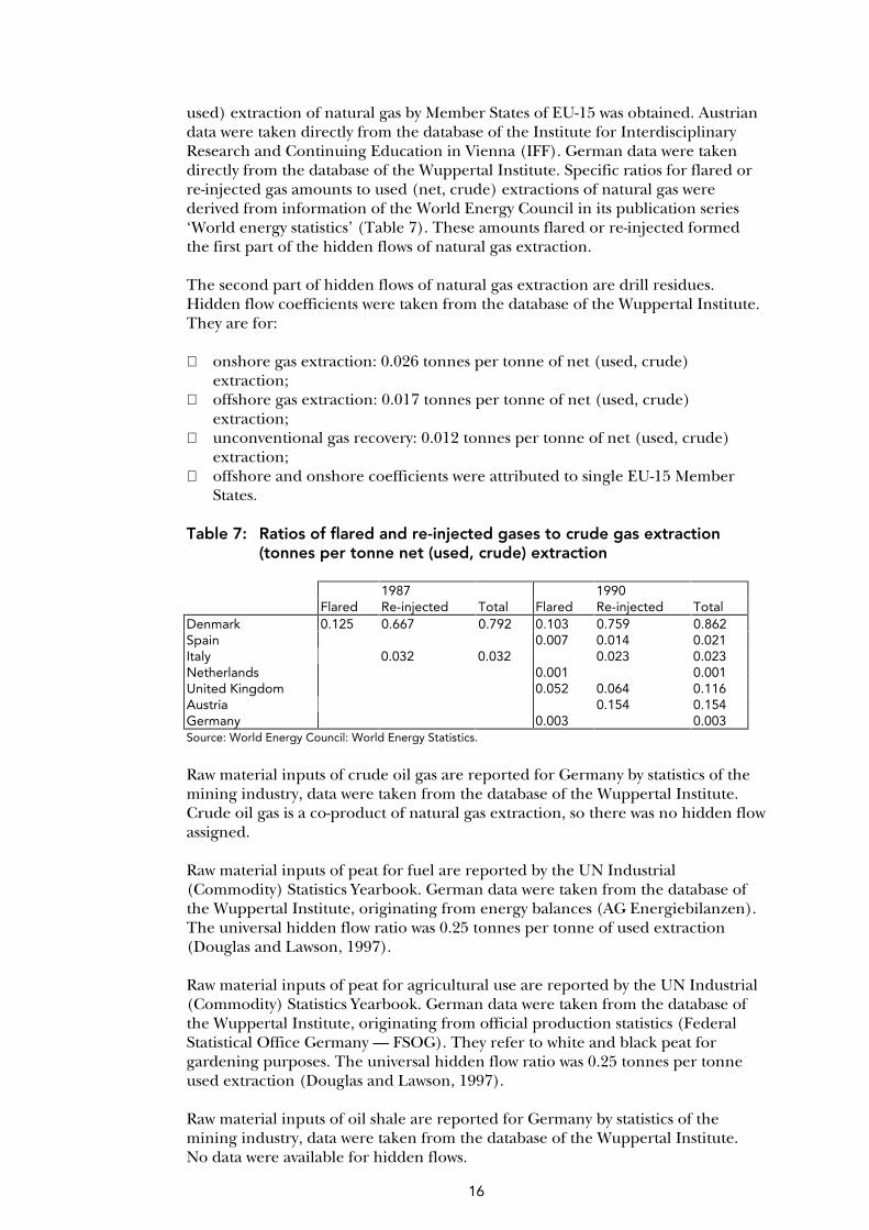
used) extraction of natural gas by Member States of EU-15 was obtained. Austrian data were taken directly from the database of the Institute for Interdisciplinary Research and Continuing Education in Vienna (IFF). German data were taken directly from the database of the Wuppertal Institute. Specific ratios for flared or re-injected gas amounts to used (net, crude) extractions of natural gas were derived from information of the World Energy Council in its publication series ‘World energy statistics’ (Table 7). These amounts flared or re-injected formed the first part of the hidden flows of natural gas extraction. The second part of hidden flows of natural gas extraction are drill residues. Hidden flow coefficients were taken from the database of the Wuppertal Institute. They are for: onshore gas extraction: 0.026 tonnes per tonne of net (used, crude)
extraction; offshore gas extraction: 0.017 tonnes per tonne of net (used, crude)
extraction; unconventional gas recovery: 0.012 tonnes per tonne of net (used, crude)
extraction; offshore and onshore coefficients were attributed to single EU-15 Member
States. Table 7: Ratios of flared and re-injected gases to crude gas extraction (tonnes per tonne net (used, crude) extraction 1987 1990 Flared Re-injected Total Flared Re-injected Total Denmark 0.125 0.667 0.792 0.103 0.759 0.862 Spain 0.007 0.014 0.021 Italy 0.032 0.032 0.023 0.023 Netherlands 0.001 0.001 United Kingdom 0.052 0.064 0.116 Austria 0.154 0.154 Germany 0.003 0.003 Source: World Energy Council: World Energy Statistics.
Raw material inputs of crude oil gas are reported for Germany by statistics of the mining industry, data were taken from the database of the Wuppertal Institute. Crude oil gas is a co-product of natural gas extraction, so there was no hidden flow assigned. Raw material inputs of peat for fuel are reported by the UN Industrial (Commodity) Statistics Yearbook. German data were taken from the database of the Wuppertal Institute, originating from energy balances (AG Energiebilanzen). The universal hidden flow ratio was 0.25 tonnes per tonne of used extraction (Douglas and Lawson, 1997). Raw material inputs of peat for agricultural use are reported by the UN Industrial (Commodity) Statistics Yearbook. German data were taken from the database of the Wuppertal Institute, originating from official production statistics (Federal Statistical Office Germany — FSOG). They refer to white and black peat for gardening purposes. The universal hidden flow ratio was 0.25 tonnes per tonne used extraction (Douglas and Lawson, 1997). Raw material inputs of oil shale are reported for Germany by statistics of the mining industry, data were taken from the database of the Wuppertal Institute. No data were available for hidden flows.

17
2.5. Minerals
This group of domestic raw materials comprises non-energy and non-metallic minerals which are counted under fossil energy carriers, respectively ores. The minerals group is organised in the following worksheets: 00: Commodities/sources; 01: Minerals A, C, E/domestic; 02: Minerals B/domestic; 03: Minerals D/domestic; 04: Minerals/phosphate/domestic; 05: Minerals/potash/domestic; 06: Minerals/salts/domestic; 07: Minerals/barytes/domestic; 08: Minerals/fluorspar/domestic; 09: Minerals/asbestos/domestic; 10: Minerals/magnesite/domestic; 11: Minerals/borates/domestic; 12: Minerals/arsenic/domestic; 13: Minerals/abrasives/domestic; 14: Minerals/graphite/domestic; 15: Minerals/mica/domestic; 16: Minerals/other/domestic. Worksheet 17, ‘Minerals/summary/domestic’, takes up the results of worksheets 1 to 16, and from there transfers summary tables by automatic link to the final data compilation in workbook ‘TMR data summary’. A general overview of the accounting of minerals by commodities and data sources is given in the worksheet 00 ‘Commodities/sources’ (Table 8). Accounting for EU-15 was based on two data sources: (1) European Minerals Yearbook (EMY), 2nd Edition, 1998, available on the web page of DG III, and (2) UN Industrial Statistics Yearbook (ISY), 1990, 1992. In order to make the accounting compatible with the elaborated material flow accounts in Germany (Environmental and Economic Accounting series of FSOG, and the Wuppertal Institute), five classes A, B, C, D and E were introduced and categories in Table 8 were allocated to these: A Sand and gravel. B Limestone and dolomite. C Natural stones. D Clays. E Other crude and broken natural stones. The remaining categories were treated as single accounting identities. Table 8 further shows some remarks on the categories available from EMY and ISY. For example, domestic cement and lime produced are not raw materials, but processed outputs, made from domestic and/or foreign raw materials. Time series of material inputs of minerals were available by EMY until 1995, and time series for 1996 and 1997 had to be established. Data for 1996 and 1997 were available for Germany (Wuppertal Institute) and Finland (Thule Institute at University of Oulu, Finland; Juutinen and Mäenpää, 1999) from their specific databases. Data for 1996 were available for Austria (database of the Institute for Interdisciplinary Research and Continuing Education in Vienna — IFF). Data for

18
the remaining years and other EU Member States were estimated by analysing the past trend of the single commodity inputs and continuing it for 1996 and 1997. Raw material inputs of classes A, C and E were presented in worksheet 01 ‘Minerals A, C, E/domestic’. The following individual positions were counted: crushed rock aggregates; sand and gravel; dimension stone; slate; gypsum and anhydrite; sulphur; diatomite; feldspar; perlite; quartz and quartzite; silica sand; talc (and steatite). With the exception of slate (UN-ISY), all data were from EMY, no data were available for quartz and quartzite. Comparing the total of these 12 categories for Germany with the corresponding total material input in the original German database, the former were by 5 % to 20 % lower. This seems to be quite acceptable. Still, in the worksheet, final data for Germany were replaced with the original ones.

19
Table 8: Accounting of minerals by commodities and data sources.
Ratios of hidden flows to commodity inputs for minerals A, C, E were taken mostly from the database of the Wuppertal Institute as follows (in tonnes of hidden flows per tonne of commodity):
crushed rock aggregates: 0.23; sand and gravel: 0.14; dimension stone: 0.23; slate: 0.1 to 0.22, applied only for Germany; gypsum and anhydrite: not available; sulphur not available, in Germany a by-product
of natural gas; diatomite: 0.7 to 1.5, applied only for Germany; feldspar: 0.004 to 0.008, applied only for
Germany; perlite not available; quartz and quartzite no data for raw material input available;
Classifications and data for minerals1. European Minerals Yearbook, 2nd Edition, 1998 2. UN Industrial Statistics Yearbook, 1990, 1992Positions: Classes Positions: Classes
1 Crushed Rock Aggregates C 1 Gravel and crushed stone A,C2 Sand and Gravel A 2 Sand, silica and quartz A3 Dimension stones C 3 Marble, travertines etc. C4 Calcium carbonate and dolomite B 4 Granite, porphyry, basalt, sandstone etc. C
5 Limestone and calcerous stone B6 Dolomite B7 Chalk C
5 Slate C 8 Slate C6 Common or structural clays D 9 Clays, total production D7 Cement8 Gypsum and Anhydrite C 10 Gypsum C9 Lime
10 Phosphate rock 11 Natural phosphates11 Potash 12 Potash12 Salt 13 Salt unrefined13 Sulphur C 14 Sulphur C14 Barite 15 Barytes15 Fluorspar 16 Fluorspar16 Kaolin D17 Refractory clays and Sillimanite minerals D18 Bentonite, Sepiolite and Attapulgite D19 Asbestos 17 Asbestos20 Diatomite E21 Feldspar C22 Magnesite 18 Magnesite23 Perlite E24 Quartz and Quartzite A,C25 Silica sand A26 Talc E 19 Talc E
20 Borate minerals21 Arsenic22 Abrasives23 Graphite24 Diamonds, industrial25 Diamonds, gems26 Mica27 Peat for fuel28 Peat for agricultural use
Classes:Source: German Production and Mining Statistics
ClassesA Sand and GravelB Limestone and DolomiteC Natural stonesD ClaysE Other crude and broken natural stones
Commodities not found here (but in German sources):Oil shaleOther products from mining and similar products
Remarks: Remarks:
12/3 sedimentary rocks (limestone, dolomite), other 1/3:igneous rock (basalt, diabase etc.) or metamorphic rock(gneiss, marble, quartzite, schist, slate, etc.)
1
2 23 Marble and Granite 34 45 No Data 5 excl. dolomite and chalk6 6 No Data7 Not a Raw Material ! 78 8 excl. roofing slate9 Not a Raw Material ! 9 contains 6, 16, 17 and 18 of EMY-categories
10 1011 1112 1213 1314 1415 1516 1617 Sillimanite, kyanite, andalusite and other polymorphs 1718 1819 1920 20 Germany: data possibly in other aggregates21 21 By-product of nickel, silver, pyrites
22 22 Puzzolan, pumice, volcanic cinder, Germany: data possiblyin other aggregates
23 2324 No Data 24 No Extraction in EU-1525 25 No Extraction in EU-1526 incl. soapstone 26 Al-silicates
2728

20
silica sand 0.00018 in 1991; 0.012 in 1993, applied only in Germany;
talc (and steatite) around 0.45, applied only for Germany. For the first three, quantitatively dominating materials, hidden flows were calculated at EU-15 level. As for direct material inputs, the German numbers obtained from the accounting described were subsequently replaced with the original ones. Raw material inputs of class B were presented in worksheet 02 ‘Minerals B/domestic’. In this instance, the EMY does not provide data and indicates that there are ‘no reliable statistics available’. Data were therefore taken from the UN-ISY. However, restrictions for time series in that case were even more serious than for minerals A, C, E, because data were available only until 1992. Data for 1993 to 1997 were available for Germany (database of the Wuppertal Institute, originating from official production statistics of FSOG). Data for the remaining years and other EU Member States were estimated by analysing the past trend of the single commodity inputs and continuing it for 1993 to 1997. The ratio of hidden flows to limestone and dolomite was taken from the database of the Wuppertal Institute, it is 0.33 tonnes per tonne. Raw material inputs of class D, i.e. clays, were presented in worksheet 03 ‘Minerals D/domestic’. The UN industrial commodity statistics yearbook (UN-ICSY) reports total production of clays from 1985 to 1992. The European Minerals Yearbook (EMY) reports data on four positions of clays, i.e. common or structural clays, kaolin, refractory clays and sillimanite minerals, and bentonite, sepiolite and attapulgite, which were added to total clays. For the accounting of domestic inputs of clays in EU-15, the two data sets were combined in a first step, using data from the UN-ICSY from 1985 to 1992, and data from EMY from 1993 to 1995. The resulting data therefore represented the total of clays reported by official international statistics. Regarding the accounting of used extraction of clays by EU-15, the official data for the total were checked for consistency by a step-by-step procedure, taking into account that clays typically consist of two main groups, special clays for industrial manufacturing (like kaolin), and common clays for construction materials (like bricks). First, the material inputs of special clays were divided into the following groups (named sub-positions 1 to 4 of position 1, i.e. total clays, in the worksheet): bentonite (UN-ICSY), and bentonite, sepiolite and attapulgite (EMY); fuller’s earth (UN-ICSY); kaolin (UN-ICSY; EMY); andalusite, kyanite and sillimanite (UN-ICSY), and refractory clays and
sillimanite minerals (EMY). Second, the sum of these four clays was subtracted from the total input of clays obtained as described before. Using the same statistical sources, the difference between total clay input and the four types of special clays therefore resulted in the material input of other clays, assumed to be identical with common clays for construction materials (sub-position 5 of position 1 in the worksheet). Third, data thus obtained for the input of common clays for construction materials were checked for consistency using the following procedure: the amount of clays necessary for the production of construction materials was estimated from data on the production of these materials and the corresponding input of clays.

21
The production of construction materials from clays was accounted for the following products (all data from UN-ICSY): building bricks, made of clay (ISIC 3691-01B); tiles, roofing, made of clay (ISIC 3691-04A); tiles, roofing, made of clay (ISIC 3691-04B). Original data for these three support-positions were given in 1 000 m3 (some data are given directly in 1 000 tonnes), million units, and million m2 respectively. They were converted to tonnes by the following coefficients (derived from German production statistics of FSOG): 2 tonnes per m3, 2.73 kg per unit, and 220 kg per m2. The raw material input of clay for the production of bricks and tiles was accounted by the following coefficients (Klinnert, 1993): 1.1 tonnes of clay per tonne of bricks, and 1.0 tonnes of clay per tonne of tiles. Then, the resulting clay input for the production of the three sub-positions was added up. This sum was subtracted from the numbers obtained for the input of clays for construction materials as described before (sub-position 5 of position 1 in the worksheet). So, in an ideal case, the difference should be (close to) zero. Fourth, for a synthesis of the described accounting results, the following conventions were set up: special clays were accounted for separately: bentonite, fuller’s earth, kaolin,
andalusite etc. (step 1); common clay for the production of bricks and tiles is accounted for as
described above (step 3), but data are taken only if they are higher than those resulting from the difference between total clays and special clays (step 2).
Data obtained following rules 1 and 2 represented the used extraction of all clays in EU-15 (total clay input). Finally, data for the inputs of clays for Germany (Wuppertal Institute), Austria (Institute for Interdisciplinary Research and Continuing Education in Vienna — IFF) and the Netherlands (resource flows study — Adriaanse et al., 1997) were replaced by data from original country studies. To account for the hidden flows of clays, the following coefficients were used (in tonnes of hidden flows per tonne commodity): bentonite: not available; fuller’s earth: 0.004 to 0.017, applied only for Germany; kaolin: 0.57 to 1.78 for Germany, 8 for the UK; andalusite, kyanite and sillimanite, refractory clays: not available; common (other) clays: 0.31 to 0.36 for Germany, 0.25 for other EU Member
States. Raw material inputs of natural phosphates were presented in worksheet 04 ‘Minerals/phosphate/domestic’. Data in gross weights were taken from UN-ICSY (1985 to 1992), EMY (1993–95), and Statistical Yearbook for Foreign Countries of FSOG (1996–97). A universal coefficient of 12.02 was used to account for hidden flows (weighted average for global extraction by open-pit mining and other types of mining; source: Krauss, H., Saam, H.G., Scjmidt, H.W., ‘Phosphate — Summary report’). Raw material inputs of crude potash salts were presented in worksheet 05 ‘Minerals/potash/domestic’. Data were taken from the UN-ICSY (1985–92) and

22
from EMY (1993–95). German data were compared with numbers from official German statistics (production statistics of FSOG, mining statistics of the mining authorities of the Länder, annual reports of the German Federal Institution of Geosciences and Raw Materials) reporting on: potash crude salts extraction: total; potash crude salts extraction: used; potash crude salts extraction: K2O-content; potash salts extraction marketable: K2O-content. Thus, it was found out that values for Germany in UN statistics until 1992 and in EMY from 1993 on referred to crude extraction in K2O-content, and values in EMY for West-Germany from 1986 to 1990 refer to marketable K2O-contents only. German data were then replaced by the official ones for the extraction of used crude salts. Because data of UN and EMY for France were characterised as recovered quantities of K2O, the average German multiplier to account for total used extraction was applied to derive the used extraction of potash salts in France. The coefficients for hidden flows in Germany (in tonnes of hidden flows per tonne commodity) were between 3.6 and 5.7. Only hidden flows for Germany were counted. Raw material inputs of crude salts were presented in worksheet 06 ‘Minerals/salts/domestic’. Data were taken from the UN-ICSY and from EMY. German data were replaced by numbers from official German statistics (production statistics of FSOG, mining statistics of the mining authorities of the Länder, annual reports of the German Federal Institution of Geosciences and Raw Materials) reporting on rock salt, industrial brine and boiled salt. The coefficients for hidden flows in Germany (in tonnes of hidden flows per tonne of commodity) were between 0.034 and 0.055. Only hidden flows for Germany were counted. Raw material inputs of barytes were presented in worksheet 07 ‘Minerals/barytes/domestic’. Data were taken from the UN-ICSY (1985–90) and from EMY (1991–95). German data were compared with numbers from official German statistics (production statistics of FSOG, mining statistics of the mining authorities of the Länder, annual reports of the German Federal Institution of Geosciences and Raw Materials) reporting on total and used extractions. The coefficients for hidden flows in Germany (in tonnes of hidden flows per tonne of commodity) were between 0.36 and 0.78, only hidden flows for Germany were counted. Raw material inputs of fluorspar (excluding precious stones) were presented in worksheet 08 ‘Minerals/fluorspar/domestic’. Data were taken from the UN-ICSY and from EMY. German data were replaced by numbers from official German statistics (production statistics of FSOG, mining statistics of the mining authorities of the Länder, annual reports of the German Federal Institution of Geosciences and Raw Materials) reporting on total and used extractions. The coefficients for hidden flows in Germany (in tonnes of hidden flows per tonne of commodity) were between 1.03 and 1.76. Only hidden flows for Germany were counted. Raw material inputs of asbestos were presented in worksheet 09 ‘Minerals/asbestos/domestic’. Data were taken from the UN-ICSY and from EMY. No hidden flows were counted.

23
Raw material inputs of magnesite were presented in worksheet 10 ‘Minerals/magnesite/domestic’. Data were taken from the UN-ICSY and from EMY. No hidden flows were counted. Raw material inputs of crude borate minerals were presented in worksheet 11 ‘Minerals/borates/domestic’. Data were taken from the UN-ICSY. No hidden flows were counted. Raw material inputs of arsenic were presented in worksheet 12 ‘Minerals/arsenic/domestic’. Data were taken from the UN-ICSY. No data were reported for EU-15. Raw material inputs of natural abrasives (pozzolan, pumice, etc.) were presented in worksheet 13 ‘Minerals/abrasives/domestic’. Data were taken from the UN-ICSY. No hidden flows were counted. Raw material inputs of natural graphite were presented in worksheet 14 ‘Minerals/graphite/domestic’. Data were taken from the UN-ICSY. German data were replaced by figures from official German statistics (production statistics of FSOG, mining statistics of the mining authorities of the Länder, annual reports of the German Federal Institution of Geosciences and Raw Materials) reporting on total and used extractions. The coefficients for hidden flows in Germany (in tonnes of hidden flows per tonne commodity) were between 0.63 and 0.88. Only hidden flows for Germany were counted. Raw material inputs of mica were presented in worksheet 15 ‘Minerals/mica/domestic’. Data were taken from the UN-ICSY. No hidden flows were counted. Raw material inputs of other minerals were presented in worksheet 16 ‘Minerals/other/domestic’. This concerns only German data taken from official German statistics (production statistics of FSOG). No hidden flows were counted.
2.6. Ores
This group of domestic raw materials comprises metallic minerals. It is organised in the following worksheets: 01: Ores/iron/domestic; 02: Ores/copper/domestic; 03: Ores/zinc/domestic; 04: Ores/lead/domestic; 05: Ores/bauxite/domestic; 06: Ores/tin/domestic; 07: Ores/tungsten/domestic; 08: Ores/vanadium/domestic; 09: Ores/manganese/domestic; 10: Ores/chromium/domestic; 11: Ores/nickel/domestic; 12: Ores/titanium/domestic; 13: Ores/silver/domestic; 14: Ores/gold/domestic; 15: Ores/tantalum/niobium/domestic; 16: Ores/antimony/domestic; 17: Ores/cobalt/domestic;
24
18: Ores/mercury/domestic; 19: Ores/uranium/domestic; 20: Ores/pyrite/pyrrhotite/domestic. Worksheet 21, ‘Ores/summary/domestic’, takes up the results of worksheets 01 to 20, and transfers summary tables by automatic link to the final data compilation in workbook ‘TMR data summary’. For the accounting of ores, a basic convention with respect to used and unused extractions has to be made. In most statistics, mine production of metallic minerals is given in weight units of the pure metal content. This is of course far from the situation of the raw materials extracted in mines and used for further purification by smelting and refining. It is even far from an intermediate product often produced within the integrated unit of mining and smelting, for example metal concentrates. And it may still be inconsistent even with the highest purity of metal achieved at the final stage of manufacturing. In order to overcome the problem of defining at which quality level, i.e. the grade of metal content of the marketed product leaving the primary production sector, metallic minerals are marketed, it was decided in this study to account for the total mass of metallic mineral in its virgin state as the used extraction of the commodity. So, used extraction, in this case, comprises the metal content plus the ancillary mass of the crude ore. They are counted by multiplying the metal content in tonnes by 100 divided by the metal grade in %. Hidden flows or unused extractions, in this case, are additional overburden or rock removed to extract the crude ore. Raw material inputs of iron ores were presented in worksheet 01, ‘Ores/iron/domestic’. Data reported in actual weights were taken from the UN-ICSY (1985–92), EMY (1993–95), and Statistical Yearbook for Foreign Countries of FSOG (1996–97). German data were replaced with numbers from official German statistics (production statistics of FSOG, mining statistics of the mining authorities of the Länder, annual reports of the German Federal Institution of Geosciences and Raw Materials). Data for Austria were replaced by the database of the Institute for Interdisciplinary Research and Continuing Education in Vienna (IFF). A universal hidden flow coefficient of 1.38 (in tonnes of hidden flows per tonne of commodity) was used referring to the situation in Brazil and Canada (Merten et al., 1995). Raw material inputs of copper ores were presented in worksheet 02 ‘Ores/copper/domestic’. Data reported in metal contents were taken from the UN-ICSY (1985–92), EMY (1993–95), and Statistical Yearbook for Foreign Countries of FSOG (1996–97). Copper grades of ores (in %) were taken from the database of the World Resources Institute (WRI — personal communication, based on publications of the US Bureau of Mines). They were available for Spain, Portugal, Sweden and Finland, representing between 88 % and 100 % of the total EU-15 metal contents. For other Member States, the average global grades of copper ores were applied. To account for hidden flows of copper ores, the following information was used (also from WRI): stripping ratio (open-pit) in tonnes overburden per tonne usable extraction; open pit in % of total copper mining. These two parameters were available for Spain and Sweden, representing between 74 % and 94 % of total used extractions in EU-15. No such hidden flows were counted for other Member States. For underground mining, a minimum rucksack

25
ratio of 0.1 tonnes of unused extraction per tonne of used extraction was assumed for all Member States of EU-15. Raw material inputs of zinc ores were presented in worksheet 03 ‘Ores/zinc/domestic’. Data reported in metal contents were taken from the UN-ICSY (1985–92), EMY (1993–95), and Statistical Yearbook for Foreign Countries of FSOG (1996–97). Zinc grades of ores (in %) were taken from EMY and from a publication of the US Bureau of Mines (BOM, 1993). To account for hidden flows of zinc ores in Germany, official data from the mining statistics of the mining authorities of the Länder were used. For other EU Member States, a minimum rucksack ratio of 0.1 tonnes of unused extraction per tonne of used extraction was assumed. Raw material inputs of lead ores were presented in worksheet 04 ‘Ores/lead/domestic’. Data reported in metal contents were taken from UN-ICSY (1985–92), EMY (1993–95), and Statistical Yearbook for Foreign Countries of FSOG (1996–97). Lead grades of ores (in %) were taken from EMY and from a publication of the US Bureau of Mines (BOM, 1993). To account for hidden flows of lead ores in Germany, official data from the mining statistics of the mining authorities of the Länder were used. For other EU Member States, a minimum rucksack ratio of 0.1 tonnes of unused extraction per tonne of used extraction was assumed. Raw material inputs of aluminium ores (bauxite) were presented in worksheet 05, ‘Ores/bauxite/domestic’. Data reported in gross weights of crude ore mined were taken from the UN-ICSY (1985–92), EMY (1993–95), and the Statistical Yearbook for Foreign Countries of FSOG (1996–97). German data were taken from official German statistics (production statistics of FSOG, mining statistics of the mining authorities of the Länder, annual reports of the German Federal Institution of Geosciences and Raw Materials). Hidden flow coefficients (in tonnes of overburden per tonne of bauxite) were available specifically for Greece (Rohn et al., 1995) and for the global average (Adriaanse et al., 1997) which was used for other EU Member States. Raw material inputs of tin ores were presented in worksheet 06 ‘Ores/tin/domestic’. Data reported in metal contents from taken from the UN-ICSY (1985–92), EMY (1993–95), and Statistical Yearbook for Foreign Countries of FSOG (1996–97). Tin grades of ores (in %) were taken from Young (1993) for a global average and from a publication of the US Bureau of Mines (BOM, 1986) for the UK. A minimum rucksack ratio of 0.1 tonnes of unused extraction per tonne of used extraction was assumed to account for hidden flows. Raw material inputs of tungsten ores were presented in worksheet 07 ‘Ores/tungsten/domestic’. Data reported in metal contents were taken from the UN-ICSY (1985–92), and EMY (1993–95). Tungsten grades of ores (in %) were taken for Austria, France, Portugal, Spain, Sweden and the UK from a publication of the US Bureau of Mines (BOM, 1985) and from Gocht (1985) for a global average. A minimum rucksack ratio of 0.1 tonnes of unused extraction per tonne of used extraction was assumed to account for hidden flows. Raw material inputs of vanadium ores were presented in worksheet 08 ‘Ores/vanadium/domestic’. Data reported in metal contents were taken from the UN-ICSY (1985–92). Finland is the only EU member concerned and data are reported for one year: 1985. Vanadium grades of ores (in %) were taken from Gocht (1985) for crude ores in South Africa. A minimum rucksack ratio of 0.1
26
tonnes of unused extraction per tonne of used extraction was assumed to account for hidden flows. Raw material inputs of manganese ores were presented in worksheet 09 ‘Ores/manganese/domestic’. Data given in actual weights were taken from Unctad for 1985 (Commodity Yearbook) and EMY for 1986 to 1995. A minimum rucksack ratio of 0.1 tonnes of unused extraction per tonne of used extraction was assumed to account for hidden flows. Raw material inputs of chromium ores were presented in worksheet 10 ‘Ores/chromium/domestic’. Data reported in metal contents were taken form the UN-ICSY (1985–92) and in gross weights by EMY (1986–95). A minimum rucksack ratio of 0.1 tonnes of unused extraction per tonne of used extraction was assumed to account for hidden flows. Raw material inputs of nickel ores were presented in worksheet 11 ‘Ores/nickel/domestic’. Data reported in metal contents were taken from the UN-ICSY (1985–92), EMY (1993–95), and Statistical Yearbook for Foreign Countries of FSOG (1996–97). Nickel grades of ores (in %) were taken for Finland and Greece from a publication of the US Bureau of Mines (BOM, 1984) and from Young (1993) for a global average. A minimum rucksack ratio of 0.1 tonnes of unused extraction per tonne of used extraction was assumed to account for hidden flows. Raw material inputs of titanium ores were presented in worksheet 12 ‘Ores/titanium/domestic’. Data reported in gross weights of ilmenite concentrates were taken from the UN-ICSY (1985–92) and EMY (1993–95). According to EMY, at least 36 % titanium is found in concentrates from ilmenite. Nickel grades of ores (in %) were taken for Finland and Italy from a publication of the US Bureau of Mines (BOM, 1986) and from Gocht (1985) for a global average of titanium in ilmenite sands. A minimum rucksack ratio of 0.1 tonnes of unused extraction per tonne of used extraction was assumed to account for hidden flows. Raw material inputs of silver ores were presented in worksheet 13 ‘Ores/silver/domestic’. Data reported in metal contents were taken from the UN-ICSY (1985–92), EMY (1993–95), and Statistical Yearbook for Foreign Countries of FSOG (1996–97). Silver grades of ores (in %) were taken for Finland, France, Italy, Spain and Sweden from a publication of the US Bureau of Mines (BOM, 1986) and from Wilmouth et al. (1991) for a global average. A rucksack ratio of 1.25 tonnes of unused extraction per tonne of used extraction was assumed to account for hidden flows. Raw material inputs of gold ores were presented in worksheet 14 ‘Ores/gold/domestic’. Data reported in metal contents were taken from the UN-ICSY (1985–92), EMY (1993–95), and Statistical Yearbook for Foreign Countries of FSOG (1996–97). Gold grades of ores (in %) were taken from Young (1993) for a global average. A minimum rucksack ratio of 0.1 tonnes of unused extraction per tonne of used extraction was assumed to account for hidden flows. Raw material inputs of tantalum and niobium ores were presented in worksheet 15 ‘Ores/tantalum/niobium/domestic’. Data reported in gross weights of concentrates were taken from the UN-ICSY (1985–92). No hidden flows were counted.

27
Raw material inputs of antimony ores were presented in worksheet 16 ‘Ores/antimony/domestic’. Data reported in metal contents were taken from the UN-ICSY (1985–92). Antimony grades of ores (in %) were taken from Gocht (1985) for the average in rich, sulphuric ores. A minimum rucksack ratio of 0.1 tonnes of unused extraction per tonne of used extraction was assumed to account for hidden flows. Raw material inputs of cobalt ores were presented in worksheet 17 ‘Ores/cobalt/domestic’. Data reported in metal contents of ores and concentrates were taken from the UN-ICSY (1985–92). No hidden flows were counted. Raw material inputs of mercury ores were presented in worksheet 18 ‘Ores/mercury/domestic’. Data reported in metal contents recovered from ores and concentrates were taken from the UN-ICSY (1985–92). Mercury grades of ores (in %) were taken from Wilmouth et al. (1991) for a global average. A minimum rucksack ratio of 0.1 tonnes of unused extraction per tonne of used extraction was assumed to account for hidden flows. Raw material inputs of uranium ores were presented in worksheet 19 ‘Ores/uranium/domestic’. Data reported in metal contents of ores and concentrates were taken from the UN-ICSY (1985–92). German data were taken from official German statistics (mining statistics of the mining authorities of the Länder). Uranium grades of ores (in %) were taken from Manstein (1995) for a global average. Rucksack ratios of 1.9 tonnes of unused extraction per tonne of used extraction were used for underground mining and 30 t/t for open-pit mining (Manstein, 1995, open-pit was attributed to the former East Germany) to account for hidden flows. Raw material inputs of pyrite and pyrrhotite were presented in worksheet 20 ‘Ores/pyrite/pyrrhotite/domestic’. Data reported in gross weights were taken from the UN-ICSY (1985–92), EMY (1993–95), and Statistical Yearbook for Foreign Countries of FSOG (1996–97). The coefficients for hidden flows in Germany (in tonnes of hidden flows per tonne of commodity) were between 0.7 and 1.2. Only hidden flows for Germany were counted.

28
3. Foreign material flows
The following chapters will give descriptions of data and methods for the step-by-step accounting of foreign material flows of EU-15 as shown in the upper right hand side of Figure 1. Its major components are organised in the following files: 00: Imports/general; 01: Imports/agriculture/raw; 02: Imports/forestry/raw; 03: Imports/animals/raw products; 04: Imports/agricult./plant product; 05: Imports/agricult./animal product; 06: Imports/forestry/semi; 07: Imports/forestry/finished; 08: Imports/biotic products; 09: Imports/fossils/raw; 10: Imports/metalsr/aw; 11: Imports/minerals/raw; 12: Imports/fossils/semi; 13: Imports/metals/semi; 14: Imports/minerals/semi; 15: Imports/metals/finished; 16: Imports/minerals/finished; 17: Imports/abiotic products; 18: Imports/other products; 19: EU12/Imports/1988–94; Summary. Data for extra-EU imports of commodities (in tonnes and ECU) from 1988 to 1997 were downloaded from the electronic database of Eurostat on CD-ROM (© ECSC-EC-EAEC, 1998). The only exception from this source were data for commodity 2716, electricity. Data extracted for 2716 from the CD-ROM were reported in tonnes which, of course, does not make sense. The correct unit of measure, however, could not be identified. Therefore, data for imported electricity by the EU were taken from OECD energy statistics series reported there in GWh. At the beginning of this study, data for EU-15 from 1995 to 1997 were collected. Later on it was decided to extend the time series with imports on EU-12 from 1988 to 1994. Therefore, these data were collected in file 19, named ‘EU-12/imports/1988–94’. As already mentioned in the beginning, it has to be considered further that data for EU-12 exclude imports by the former GDR from 1988 to 1990, but include these imports since 1991 within the re-united Germany. As can be seen from the list of files 01 to 18 for the categorisation of imports, the overall aim of this exercise was to distinguish between raw materials, semi-manufactured products and finished products. TMR accounts on the international level so far comprised hidden flows of raw materials and semi-manufactured products, but mainly because of data restrictions, not for finished products (Adriaanse et al., 1997). Classifications of the foreign trade statistics of Eurostat, however, do not identify these three material groups. Therefore, a comparative analysis had to be performed using a comparative statement of two German official foreign trade classification systems, (a) ‘Commodities of the nutrition industry and the commercial industry’ (Waren der Ernährungswirtschaft und der

29
Gewerblichen Wirtschaft — EGW’), and (b) ‘Commodity register for foreign trade statistics’ (Warenverzeichnis für die Aussenhandelsstatistik — WA). This comparative statement was kindly provided by the Federal Statistical Office Germany (document EGW/WA, 1999). Whereas the WA classification is identical to the one made available here by Eurostat data, the EGW classification distinguishes the following four major groups: nutrition industry; commercial industry: raw materials; commercial industry: semi-manufactured products; commercial industry: finished products (with further breakdown into pre-
manufactured and final products). This means that commodities of the commercial industry can be clearly differentiated. Commodities of the nutrition industry are further differentiated by: living animals; nutritional goods originating from animals; nutritional goods originating from plants; natural stimulants (Genussmittel, i.e. coffee, tobacco, beer, etc.). The first two groups (animal products) contain raw materials in terms of material flow accounting in the form of (wild) fishes. They were classified here in two files (‘animals/raw and products’, i.e. fish, crab, molluscs and derived products, and ‘agricultural animal products’) without further distinction by semi-manufactured products and finished products. The other two groups, originating from plants, comprise both raw materials (e.g. wheat or tobacco leaves) and products (e.g. wheat flour or cigarettes). Raw materials were selected and grouped under the heading ‘agricultural raw materials’. The remaining products were not further differentiated into semi-manufactured products and finished products but grouped under the heading ‘agricultural plant products. The classification procedure of the four main groups according to the German EGW classification was documented in workbook ‘Summary’ in each of the worksheets/tables referring to the commodity groups 01 to 18 as listed above. It allocates the classification numbers of foreign trade statistics of Eurostat to the four EGW classes. File 00 ‘Imports/general’ contains two files, named ‘ECU261610/90’ and ‘FAO yields’. File ‘ECU261610/90’ contains worksheets with data of imports of commodities 261610 (silver ores and concentrates) and 261690 (precious metals ores and concentrates, excluding silver) in monetary units (1 000 ECU). The use of these data will be described later in the context of file 10 ‘Imports/metals/raw’. File ‘FAO yields’ contains worksheets with data of yields (in hg per ha) by countries for agricultural raw materials which had been downloaded from the FAO web site (http://apps.fao.org). The use of these data will be described in the context of file 01 ‘Imports/agriculture/raw’.
3.1. Agricultural raw materials
Data to account for imported agricultural raw materials and their hidden flows (erosion) are presented in file 01 ‘Imports/agriculture/raw’ in 45 workbooks. In general, the accounting is standardised by subdividing workbooks into five worksheets/tables (a) for nomenclature (Nomenklatur), (b) for FAO yields in hg per ha (Erträge), (c) for original data of extra-EU imports in tonnes (Importe), (d)

30
for land use in hectare accounted from data in the two previous sheets (Flächen), and (e) for erosion in tonnes accounted from the land-use data by multiplication with erosion rates in tonnes per hectare (Erosion) taken from the database of the Wuppertal Institute. Table 9 shows in detail which commodities (Waren) along with their classification numbers were differentiated to account for the material flows of imported agricultural raw materials. A green mark indicates that country-specific data were used (in that case yields and erosion rates) to account for the hidden flows (unused material flows).
Table 9: Accounting of imported agricultural raw materials by commodity Classification Waren Commodity 06 Lebende Pflanzen etc. Living plants etc. 07 Gemüse Vegetable 0801-10,-11,-19 Kokosnüsse Coconuts 0802-21,-22 Haselnüsse Hazelnuts 0802-31,-32 Walnüsse Walnuts 0803 Bananen Bananas 0805 Zitrusfrüchte Citrus fruit 0806 Trauben Grapes 080810 Äpfel Apple 080920 Kirschen Cherries 080940 Pflaumen Prunes 0810 Beerenfrüchte etc. Berries etc. 08Rest Andere Früchte und Nüsse etc. Other fruit and nuts, etc. 090111 Kaffee Coffee 0902 Tee Tea 0903 Mate Mate 0904to0910 Gewürze Spices 1001 Weizen Wheat 1002 Roggen Rye 1003 Gerste Barley 1004 Hafer Oat 1005 Mais Maize 1006 Reis Rice 1007 Sorghum Sorghum 1008 Anderes Getreide Other cereals 1201 Sojabohnen Soy beans 1203 Kopra Copra 1204 Leinsamen Linseed 1205 Rapssamen Rapeseed 1206 Sonnenblumenkerne Sunflowerseed 1210 Hopfen Hops 12Rest Andere Ölsaaten etc. Other oilseeds etc. 1301 Schellack, Gummen, Harze etc. Shellac, rubber, resin, etc. 1302 Andere Pflanzensäfte und -auszüge Other plant juices and extracts 14 Flechtstoffe etc. Plant fibres etc. 1801 Kakao Cocoa 2401 Tabak Tobacco 4001 Naturkautschuk Natural rubber 5201 Baumwolle Cotton 5301 Flachs Flax 5302 Hanf Hemp 5303 Jute Jute 5304 Sisal Sisal 5305 Kokosfasern Coconut fibre Country specific data base for unused material flows.
31
3.2. Forestry raw materials
Data to account for imported forestry raw materials are presented in file 02, ‘Imports/forestry/raw’ in 4 workbooks for the following commodities: 4401: fuel wood etc;. 4403: roundwood; 4404: wood roughly prepared etc.; 4501: natural cork. No hidden flows are counted.
3.3. Animals as raw materials and products
Data to account for imported animals raw materials and products are presented in file 03, ‘Imports/animals/raw products’, in 3 workbooks for the following commodities: fish etc;. fish products; crab/Molluscs preparations. The hidden flows of imported fish (03 and 1604) were estimated according to a study by Greenpeace (Frankfurter Rundschau of 6 November 1999), according to which 25 % of the catch is being discarded on board (by-catch).
3.4. Agricultural plant products
Data to account for imported agricultural plant products are presented in file 04, ‘Imports/agricult/plant product’, in 51 workbooks. At country-specific level, four commodities are counted with respect to land use and erosion as described for agricultural raw materials (Table 10). For most of the remaining commodities, erosion was estimated within the workbook ‘Summary imports’ in the worksheet ‘Agriculture plant products’. There, erosion coefficients for EU imports of the corresponding raw materials (e.g. wheat) were multiplied with coefficients for raw material inputs of the product (e.g. wheat flour, 1 tonne being produced from 1.28 tonnes of wheat grains), the latter coefficients were taken from the database of the Wuppertal Institute.

32
Table 10: Accounting of imported agricultural plant products by commodity Classification Waren Commodity 0901-12to-90 Kaffee, geröstet und/oder entkoeffeiniert Coffee, roasted and/or decaffeinated 1101 Weizenmehl Wheat flour 1102 Mehl von anderen Getreiden Flour of other cereals 1103 Gries/Pellets von Getreiden Groats/pellets of cereals 1104 Getreidekörner, bearbeitet Cereal grains, processed 1105 Kartoffelerzeugnisse Potato products 1106 Mehl, Gries von anderen Feldfrüchten Flour, groats of other field crops 1107 Malz Malt 1108 Stärke Starch 1109 Kleber von Weizen Wheat gluten 1701 Zucker aus Rüben und Zuckerrohr Sugar of beets and sugar cane 1702 Anderer Zucker Other sugars 1703 Zuckermelassen Sugar molasses 1704 Zuckerwaren Sugar confectioneries 1802t01806 Kakaozubereitungen Cocoa products 1901 Malzextrakt etc. Malt extract etc. 1902 Teigwaren Pastry 1903 Tapiokasago Tapioca preparations 1904 Getreidezubereitungen Cereals preparations 1905 Brot und Backwaren Bread and bakery products 2001 Gemüsezubereitungen Vegetable preparations 2002 Tomaten zubereitet Tomato preparations 2003 Pilze zubereitet Mushrooms preparations 2004 Andere Gemüse zubereitet, gefroren Other vegetables preparations, frozen 2005 Andere Gemüse zubereitet, nicht gefroren Other vegetables preparations, not frozen 2006 Früchte zubereitet mit Zucker Fruit prepared with sugar 2007 Konfitüren etc. Marmalades, jellies, etc. 2008 Fruchtkonserven Fruit conserved 2009 Fruchtsäfte Fruit juices 2101 Pflanzenauszüge Plant extracts 2203 Bier Beer 2204 Wein etc. Wine etc. 2205 Wermutwein Vermouth 2206 Apfelwein Apple wine 2207 Ethanol Ethanol 2208 Spirituosen Spirits 2209 Weinessig/Speiseessig Wine vinegar, other vinegar for nutrition 2302 Rückstände Getreide/Hülsenfrüchte Residues of cereals/pulses 2303 Rückstände Maisstärke/Zuckerrüben/Treber Residues of corn starch/sugar beets/draff, 2304 Ölkuchen Soja Oilcake soybeans 2305 Ölkuchen Erdnuss Oilcake peanuts 2306 Ölkuchen andere Ölsaaten Oilcake other oilseeds 2307 Weintrub/Weinstein Tartar 2308 Eicheln/Roßkastanien/Trester/Andere pflanzl.
Futtermittel Acorns/horse-chestnuts/skins of pressed grapes/other plant foodstuffs
2402to2403 Tabakwaren Tobacco products 5202to5212 Baumwollerzeugnisse Cotton manufactures 5306 Leinen, Garne Flax, yarn 5307 Jute, Garne Jute, yarn 5308 Andere Pflanzenfasern, Garne Other plant fibres, yarn 53Rest Gewebe aus Flachs, Jute u.a. pflanzl. Fasern Tissues of flax, jute, and other plant fibres
46 Flechtwaren und Korbmacherwaren Wickerwork and basket-maker ware Country-specific data base for unused material flows.
3.5. Agricultural animal products
Data to account for imported agricultural animal products are organised under the file 05, ‘Imports/agricult/animal products’, in 50 workbooks (Table 11). For

33
these commodities, erosion was estimated within the workbook ‘Summary imports’ in worksheet ‘Agriculture/animal products’. There, erosion coefficients for EU imports of the commodities were introduced from the database of the Wuppertal Institute. Table 11: Accounting of imported agricultural animal products by commodity Classification Waren Commodity 0101 Lebende Pferde etc. Live horses etc. 0102 Lebendes Rindvieh etc. Live bovine animals 0103 Lebende Schweine etc. Live swine etc. 0104 Lebende Schafe etc. Live sheep etc. 0105 Lebendes Geflügel etc. Live poultry etc. 0106 Andere lebende Tiere Other live animals 0201 Rindfleisch, frisch, gekühlt Bovine meat, fresh, chilled 0202 Rindfleisch, gefroren Bovine meat, frozen 0203 Schweinefleisch, frisch, gekühlt, gefroren Swine meat, fresh, chilled, frozen 0204 Schaf-Ziegen-fleisch, frisch, gekühlt, gefroren Sheep (goat meat, fresh, chilled, frozen 0205 Pferdefleisch, frisch, gekühlt, gefroren Horse meat, fresh, chilled, frozen 0206 Schlachtnebenerzeugnisse Edible offals 0207 Geflügelfleisch Poultry meat 0208 Fleisch von anderen Tieren Meat of other animals 0209 Schweine-/Geflügel-fett Swine/poultry fat 0210 Fleisch/Innereien, gesalzen, getrocknet Meat/offals, salted, dried 0401 Milch und Sahne Milk and cream 0402 Milchpulver etc. Milk powder etc. 0403 Buttermilch etc. Buttermilk etc. 0404 Molke Whey 0405 Butter Butter 0406 Käse und Quark Cheese and curd 0407 Eier Eggs 0408 Eigelb etc. Egg yolk 0409 Honig Honey 0410 Andere tierische Waren Other animal goods 1601 Würste etc. Sausages etc. 1602 Fleischzubereitungen Meat preparations 1603 Fleischextrakte Meat extracts 4101 Häute/Felle von Rind/Pferd etc. Hides/skins of bovine/horse, etc. 4102 Felle von Schaf/lamm Skins of sheep/lamb 4104 Leder von Rind/Kalb/Pferd Leather of bovine/calf/horse 4105 Leder von Schaf/Lamm Leather of sheep/lamb 4106 Leder von Ziege/Zickel Leather of goat 5001 Seidenraupenkokons Silk worm cocoons 5002 Grege Grege 5003 Abfälle von Seide Silk wastes 5004 Seidengarne Silk yarns 5005 Seidengarne Silk yarns 5006 Seidengarne Silk yarns 5007 Seidengewebe Silk weaves 5101 Wolle Wool 5102 Tierhaare Animals hair 5103 Abfälle von Wolle Wool wastes 5104 Reissspinnstoffe aus Wolle Wool textile fibre 5105 Wolle gekämmt Wool combed 5106 Wollgarne Wool yarns 5107 Wollgarne Wool yarns 5108 Wollgarne Wool yarns 5109 Wollgarne Wool yarns 5110 Wollgarne Wool yarns 5111 to 5113 Wollgewebe Wool tissue

34
3.6. Forestry semi-manufactured products
Data to account for imported semi-manufactured products from forestry are presented in file 06, ‘Imports/forestry/semi’, by the following commodities: charcoal; wood-wool; sleepers; sawn wood; veneer; semi-manufactured products of wood. No hidden flows are counted.
3.7. Forestry finished products
Data to account for imported finished products from forestry are presented in file 07, ‘Imports/forestry/finished’, by the following commodities: 4409 to 4421: wooden products; 45 rest: cork products; paper and board; paper ware. No hidden flows are counted.
3.8. Biotic products
Data to account for imported biotic products which could not be clearly allocated to one of the material groups described before are presented in file 08, ‘Imports/biotic products’, by the following commodities: animal/plant fertilisers; other animal products etc.; animal/plant fats and oils, etc.; yeasts; sauce and preparations; soups and broths; ice cream; other food preparations; flour, pellets of meat/fish; foodstuffs preparations; hides/skins of goat/reptiles/other animals; leather of pigs/reptiles/other animals; 4108 to 4111: leather/rest; pelts, crude, complete; pelts, curried, prepared, assembled; clothing, other ware of pelts. No hidden flows are counted.

35
3.9. Fossil energy carriers, raw materials
Data to account for imported fossil energy carriers as raw materials are presented in file 09, ‘Imports/fossils/raw’, by the following commodities in individual workbooks: hard coal; brown coal (lignite); peat; crude oil; natural gas; bituminous crude materials. For peat, a hidden flow coefficient of 0.25 (tonnes per tonne of imported commodity) was used (Douglas and Lawson, 1997). The hidden flows of crude oil were accounted using a coefficient of 0.17 tonnes (abiotic materials) per tonne of oil, taken from the database of the Wuppertal Institute, Department of Material Flows and Structural Change (it can be found on the Internet: http://www.wupperinst.org/Projekte/mipsonline/download — document: MI-Werte.pdf). No hidden flows were accounted for bituminous crude materials. The hidden flows of imported hard coal were estimated using hidden flow coefficients for the following countries (database of the Wuppertal Institute, Department of Material Flows and Structural Change): Australia: 10.64; Russia and former Soviet Union: 5.13; Canada: 18.87; Colombia: 11.99; South Africa: 3.84; United States: 6.31. For all other imports a hidden flow coefficient of 0.89 was used in reference to the German value in 1990. The hidden flows of imported brown coal (lignite) were estimated using hidden flow coefficients for the following countries (database of the Wuppertal Institute, Department of Material Flows and Structural Change): Australia: 7.4; Poland: 7.4; Czech Republic: 6.6. For all other imports a hidden flow coefficient of 3.2 was used. The hidden flows of imported natural gas were estimated using hidden flow coefficients for the following countries (database of the Wuppertal Institute, Department of Material Flows and Structural Change): Russia and former Soviet Union: 0.56; Norway: 0.49. For all other imports a hidden flow coefficient of 0.2 was used (for abiotic materials, taken from the database of the Wuppertal Institute, Department of Material Flows and Structural Change (it can be found on the Internet:

36
http://www.wupperinst.org/Projekte/mipsonline/download — document: MI-Werte.pdf).
3.10. Metals, raw materials
Data to account for imported metals as raw materials (ores and concentrates) are organised under the file 10 ‘Imports/metals/raw’ by the following commodities in individual workbooks: iron ores; manganese ores; copper ores; nickel ores; cobalt ores; aluminium ores; lead ores; zinc ores; tin ores; chromium ores; tungsten ores; uranium/thorium ores; molybdenium ores; titanium ores; 26151000: zirkonium ores; 26159010: niob/tantalum ores; 26159090: vanadium ores; 261610: silver ores; 261690: precious metal ores; 261710: antimony ores; 261790: other ores, unspecified; 26rest: slags, ashes, residues, etc. The hidden flows of imported metals were estimated by a standard procedure comprising two components: ancillary mass (the part of extracted material which does not contain the metal under consideration) and overburden material (material that has to be removed in order to get access to the metal containing layers). Thus, the specific concentrations (%) of metal in the crude ore have to be known, as well as the specific concentrations (%) of metal in the traded commodity. Furthermore, the ratios of extracted raw material to crude ore have to be considered, and the ratios of overburden to crude ore. The ancillary mass is then given by dividing the metal concentration in the traded commodity by the metal concentration in the crude ore, multiplying the result with ratio of raw material extracted per crude ore, and subtracting 1 (for the own weight of the traded commodity). Overburden is counted by multiplying the total mass of raw material extracted (ancillary mass plus crude ore) by the overburden ratio. As far as possible the basic parameters for this accounting were used for single countries specifically. The hidden flows of imported iron ores and concentrates were estimated using the following basic parameters: metal contents in crude ores: BOM (1987) for specific countries, or in general
58 % (after Merten et al., 1995); metal contents in traded ores or concentrates: same as in crude ores; ratio of raw material extracted to crude ore: 1.11 (Gocht, 1985);

37
ratio of overburden to crude ore: 1.8 (Gocht, 1985). Hidden flows of imported iron ores from the United States were accounted specifically after Adriaanse et al. (1997). The hidden flows of imported manganese ores and concentrates were estimated using the following basic parameters: metal contents in crude ores: BOM (1992) for specific countries, or in general
30 % (Young, 1993); metal contents in traded ores or concentrates: BOM (1992) for specific
countries, or in general 44 % (Gocht, 1985); ratio of raw material extracted to crude ore: 1.25 (Gocht, 1985) ratio of overburden to crude ore: 1 (Gocht, 1985). The hidden flows of imported copper ores and concentrates were estimated using hidden flows coefficients on country-specific levels for Australia, Bulgaria, Canada, Chile, India, Indonesia, Mexico, Papua New Guinea, Peru, South Africa, Turkey, the United States, the former Soviet Union, Yugoslavia and Zaire (database of WRI after BOM, after Schütz, 1997). For other imports the following basic parameters were used: metal contents in crude ores (BOM, 1992); metal contents in traded ores or concentrates: in general 27 % (Gocht, 1985); ratio of raw material extracted to crude ore: 1.21 (Ayres and Ayres, 1996); ratio of overburden to crude ore: 2 (database of the Wuppertal Institute). The hidden flows of imported nickel ores and concentrates were estimated using the following basic parameters: metal contents in crude ores: BOM (1984) for specific countries, or in general
2.5 % (Young, 1993); metal contents in traded ores or concentrates: in general 15 % (Gocht, 1985); ratio of raw material extracted to crude ore: 1.36 (database of the Wuppertal
Institute); ratio of overburden to crude ore: 1.26 (Gocht, 1985). No hidden flows of imported cobalt ores and concentrates were estimated because cobalt is often associated with nickel. The hidden flows of imported aluminium ores and concentrates (bauxite) were estimated using the following basic parameters: metal contents in crude ores: BOM (1983) for specific countries, or in general
23 % (Young, 1993); metal contents in traded ores or concentrates: same as in crude ores; ratio of raw material extracted to crude ore: 1 (database of the Wuppertal
Institute); ratio of overburden to crude ore: after Rohn et al. (1995):
• Australia: 0.2; • Guinea: 0.2; • Jamaica: 0.05; • Brazil: 0.9; • India: 0.2;
38
• Surinam: 0.3; • China: 6.6; • Guyana: 7.5; • Sierra Leone: 0.1.
For other imports a ratio of 0.95 tonnes overburden per tonne of crude ore was used (database of the Wuppertal Institute). The hidden flows of imported lead ores and concentrates were estimated using the following basic parameters: metal contents in crude ores: BOM (1993) for specific countries, or 5 % in
general (Wilmouth et al., 1991); metal contents in traded ores or concentrates: 65 % (Gocht, 1985); ratio of raw material extracted to crude ore: 1.11 (Wilmouth et al., 1991); ratio of overburden to crude ore: 0.1 (assumption). Lead and zinc usually occur together at the same location, and both metals are marketed. Therefore, they were considered as co-products in this study. In order to account for the hidden flows of lead or zinc, their relative share in resource deposits were taken into account for individual countries (BOM, 1993). The hidden flows of imported zinc ores and concentrates were estimated using the following basic parameters: metal contents in crude ores: BOM (1993) for specific countries, or 3.7 % in
general (Wilmouth et al., 1991); metal contents in traded ores or concentrates: 57.5 % (Gocht, 1985); ratio of raw material extracted to crude ore: 1.11 (Wilmouth et al., 1991); ratio of overburden to crude ore: 0.1 (assumption). Lead and zinc usually occur together at the same location, and both metals are marketed. Therefore, they were considered as co-products in this study. In order to account for the hidden flows of lead or zinc, their relative share in resource deposits were taken into account for individual countries (BOM, 1993). The hidden flows of imported tin ores and concentrates were estimated using the following basic parameters: metal contents in crude ores: BOM (1986) for specific countries, or depending
on geographical information (Gocht, 1985) 1 % for deposits of primary ores (Young, 1993), and 0.36 for both deposits of primary ores and soaps within the same country; the latter coefficient (0.36) was obtained by weighing 1 % tin in primary ores by 35 % global occurrence (Gocht, 1985) and 0.016 % tin (Rohn et al., 1995) by 65 % global occurrence (Gocht, 1985);
metal contents in traded ores or concentrates: 29 % (Gocht, 1985); ratio of raw material extracted to crude ore: 1.11 (Gocht, 1985); ratio of overburden to crude ore: 0.1 (assumption). The hidden flows of imported chromium ores and concentrates were estimated using the following basic parameters: metal contents in crude ores: BOM (1993) for specific countries, or in general
17 % (Gocht, 1985);

39
metal contents in traded ores or concentrates: 31 % (Gocht, 1985), except for Kazakhstan (38 %) and for South Africa (34 %);
ratio of raw material extracted to crude ore: 1.18 (Gocht, 1985); ratio of overburden to crude ore: 1.325, obtained by equal weighing (50/50)
of ratio of underground mining (0.27 for South Africa, Liedtke et al., 1995) and ratio of open-pit mining (2.38 for Kazakhstan, Liedtke et al., 1995).
The hidden flows of imported tungsten ores and concentrates were estimated using the following basic parameters: metal contents in crude ores: BOM (1985) for specific countries, or in general
1.09 % (Gocht, 1985); metal contents in traded ores or concentrates: 52 % (Gocht, 1985); ratio of raw material extracted to crude ore: 1.18 (Gocht, 1985); ratio of overburden to crude ore: 0.1 (assumption). The hidden flows of imported uranium and thorium ores and concentrates were estimated using the following basic parameters: metal contents in crude ores: 0.2 % (Manstein, 1995); metal contents in traded ores or concentrates: 100 % (Wilmouth et al., 1991); ratio of raw material extracted to crude ore: 1 (assumption); ratio of overburden to crude ore: 16 obtained by equal weighing (50/50) of
ratio of underground mining (2, Manstein, 1995) and ratio of open-pit mining (30, Manstein, 1995).
The hidden flows of imported molybdenum ores and concentrates were estimated using the following basic parameters: metal contents in crude ores: BOM (1985) for specific countries, or in general
0.2 % (Wilmouth et al., 1991); metal contents in traded ores or concentrates: 53.9 % (Wilmouth et al., 1991); ratio of raw material extracted to crude ore: 1.11 (Wilmouth et al., 1991); ratio of overburden to crude ore: 0.1 (assumption). The hidden flows of imported titanium ores and concentrates were estimated using the following basic parameters: metal contents in crude ores: BOM (1986) for specific countries, or in general
0.52 % (Gocht, 1985); metal contents in traded ores or concentrates: 57 % (Gocht, 1985); ratio of raw material extracted to crude ore: 1.11 (Gocht, 1985); ratio of overburden to crude ore: 0.1 (assumption). No hidden flows of imported zirconium ores and concentrates were estimated because zirconium (and hafnium) is often associated with titanium. The hidden flows of imported niobium and tantalum ores and concentrates were estimated using the following basic parameters: metal contents in crude ores: in general 2 % (Gocht, 1985); metal contents in traded ores or concentrates: 40.2 % (Gocht, 1985); ratio of raw material extracted to crude ore: 1.54 (Gocht, 1985); ratio of overburden to crude ore: 0.1 (assumption).

40
The hidden flows of imported vanadium ores and concentrates were estimated using the following basic parameters: metal contents in crude ores: in general 0.95 % (Gocht, 1985); metal contents in traded ores or concentrates: 10.1 % (Gocht, 1985); ratio of raw material extracted to crude ore: 1.1 (Gocht, 1985); ratio of overburden to crude ore: 0.1 (assumption). Imported commodities of classification 26161000 are named ‘silver ores and concentrates’ in official foreign trade statistics. This implies that the value of the imports is in relation to the silver content of the ores and concentrates. Pure silver metal ingots are usually traded at 99.9 % silver content. Average annual prices for this commodity are recorded by statistics (e.g. Statistical Yearbook for Foreign Countries of FSOG). There, pure silver is a semi-manufacture with commodity No 7106. However, no direct information could be obtained for the quality or composition of the imported raw material, silver ores and concentrates. The silver content of crude ores usually is about 0.03 % (Wilmouth et al., 1991). For individual countries, the following silver contents in crude ores were determined (BOM, 1986): Canada (0.00461 %), Morocco (0.03119 %), Peru (0.01381 %), and the United States (0.01438 %). Silver in natural deposits is often associated with co-products and by-products like gold, zinc, lead and copper (BOM, 1986). These, however, in high-quality trade forms, have either an almost 100 times higher price (gold), or an almost 100 times lower price than silver (zinc, lead and copper). The range of values of imports of commodity 26161000, ‘silver ores and concentrates’, from individual countries by the EU is from about 1 000 ECU/kg (Zimbabwe and Papua New Guinea in 1988) to 0.01 ECU/kg (Norway in 1993). In the first case, it has to be assumed that imports contain even more valuable precious metals than silver (which reached an average price of USD 210 per kg at 99.9 % ingots in 1988). The latter case was exceptional with only one similar situation in 1991 when imports from Sweden had a price of 0.02 ECU/kg. For the remaining cases within the time series from 1988 to 1997, the average values of imports of commodity 26161000, ‘silver ores and concentrates’, was within the range of prices for silver or by-products (zinc, lead and copper). Clearly, the terminology of commodity 26161000, ‘silver ores and concentrates’, is misleading because it implies a homogenous material composition which can hardly be confirmed by the values in comparison with silver prices (unless crude silver ores at very low silver content are traded which does not seem to make sense). However, for the accounting of hidden flows of imported silver ores and concentrates, this finding caused significant uncertainty about which reference metal content should be assumed. The problem was solved in this study by applying a linear relationship between silver contents of imports and their values, taking the price of silver at 99.9 % ingots as the reference value. The lowest grade of silver in imported ores and concentrates was fixed at 10 %, referring to the silver content in enriched lead (Gocht, 1985). Other basic assumptions were the following: metal contents in crude ores: BOM (1986) for specific countries, or in general
0.03 % (Wilmouth et al., 1991); metal contents in traded ores or concentrates: 95 % (Gocht, 1985); ratio of raw material extracted to crude ore: 1 (assumption) ratio of overburden to crude ore: 1.25 obtained by equal weighing (50/50); of
ratio of underground mining (0.5) and ratio of open-pit mining (2).

41
Imported commodities of classification 26169000 are named ‘precious metals, ores and concentrates (excluding silver ores and concentrates)’ in official foreign trade statistics. According to Gocht (1985) precious metals, excluding silver, are gold and the platinum group metals (PGM metals), which are platinum, palladium, rhodium, iridium, osmium and ruthenium. The term precious metals, thus, implies that the value of the imports is in relation to the precious metal content of the ores and concentrates. Pure gold metal ingots are usually traded at 100 % gold content. The lowest quality of crude gold has about 80–90 % gold content (Gocht, 1985; Renner and Johns, 1989). Average annual prices for traded gold are recorded by statistics (e.g. Statistical Yearbook for Foreign Countries of FSOG). There, pure gold is a semi-manufacture with commodity No 7108 and PGM metals are semi-manufactured products with commodity No 7110. However, no direct information could be obtained for the quality or composition of the imported raw material, precious metals ores and concentrates. The average global gold content of crude ores is about 0.00033 % to 0.0004 % (Young, 1993; Wilmouth et al., 1991). For individual countries, the following gold content in crude ores were determined: Canada (0.00114 %), South Africa (0.00095 %), the United States (0.00022 %), Zimbabwe (0.00062 %) (BOM, 1986), and Papua New Guinea (0.0004 %) (Renner and Johns, 1989). Gold and PGM metals in natural deposits are often associated with co-products and by-products like silver, cobalt, copper and nickel (BOM, 1986). Prices for these compounds, however, vary greatly, e.g. for mine production in South-Africa (BOM, 1986, USD per kg): Co-products: platinum: 16 278; palladium: 4 623; rhodium: 41 737; gold: 12 241. By-products: cobalt: 19; copper 2; iridium: 9 728; nickel: 16; osmium: 17 631; ruthenium: 1 991. The range of values of imports of commodity 26169000, ‘precious metals ores and concentrates’, from individual countries by the EU is from about 10 000 ECU/kg (Indonesia, 1990, 1991, 1995–97) to 0.06 ECU/kg (Guadeloupe, 1996). In the first case, it has to be assumed that imports predominantly contained valuable precious metals (over the time period 1988–97 gold reached average prices of USD 10 647 to 14 054 per kg at 100 % ingots). The latter case of prices being lower than 0.5 ECU/kg was met in some more cases (Turkey in 1991, Finland in 1992, Argentina in 1993, India in 1994). For the remaining cases within the time series from 1988 to 1997, the average values of imports of commodity 26169000, ‘precious metals ores and concentrates’, was within the range of prices for other by-products (cobalt, copper and nickel). A specific problem occurred with data for commodity 26169000, ‘precious metals ores and concentrates’ regarding imports from Finland. The data downloaded from the Eurostat CD-ROM stated 11 424 tonnes imported by the EU from Finland in 1992, representing 77 % of the total imports in 1992 which were thereby significantly higher than in the remaining years of the time series (1988–97). Therefore, a cross-check was performed with respect to the validity of the data

42
from the Eurostat CD-ROM. First, it was confirmed by Eurostat on request that these data are correct (as downloaded). Second, the same information was asked from the official foreign trade statistics of Finland (Kari Tähtivaara, personal communication by e-mail from 25 February 2000). The latter request stated that 7 tonnes of commodity 26169000 had been exported to the EU (actually to Great Britain) in 1992 with a value of FIM 17 million (about EUR 2.8 million), so the value was about 400 EUR/kg. These 7 tonnes, thus, compare to 11 424 tonnes, and the question remains which number is right. Therefore, the data for extra-EU imports of commodity 26169000 from Finland were deleted. Clearly, the terminology of commodity 26169000, ‘precious metals ores and concentrates’, is misleading because it implies a homogenous material composition which can hardly be confirmed by the values in comparison with precious metals prices. These values rather imply that crude precious metals ores at very low precious metals content are traded. For example, in any first production step of gold ore, treatment concentration processes are used such as gravity separation, milling, amalgamation or cyanidation (Renner and Johns, 1989). Cyanidation is common, for example, in South Africa since 1890 and the whole process chain leads to raw gold with a gold content of 80–90 %. Ground gold ore that contains large gold particles or sulphides may be unsuitable for cyanidation. Pre-treatment, consisting of gravity concentration, generally followed by amalgamation, is therefore nearly always necessary. Along this process chain, gravity concentration leads to a concentrate which is further processed by amalgamation to spongy gold and finally, by melting, to gold bars. The first intermediate product of this chain is a concentrate which may contain, besides gold, silver, iron pyrites, metallic iron and water content of about 70 %. Consequently, the overall metals content in this concentrate of gold ores is below 30 %, however, the share of gold and other individual metals is unknown. Since 1970, conventional cyanide leaching has been superseded by the carbon-in-pulp process. Besides, other methods have been used in recent times, including solvent extraction methods. For the accounting of hidden flows of imported precious metals ores and concentrates, these findings caused significant uncertainty about which reference metal content should be assumed. The problem was solved in this study by applying a linear relationship between the gold contents of imports and their values, taking the price of gold at 100 % ingots as the reference value. Analogously to silver, the lowest grade of gold in imported ores and concentrates was fixed at 10 %. Other basic assumptions were the following: Metal contents in crude ores: specifically for the United States, Papua New
Guinea, Canada, Zimbabwe and South Africa (which together accounted for, e.g., 75 % of global gold mine production in 1996), or 0.0001 % for the rest of the world gold production (derived from Renner and Johns, 1989, and statistics for foreign countries of FSOG);
metal contents in traded ores or concentrates: according to prices (see above) or a minimum content of 10 %;
ratio of raw material extracted to crude ore: 1 (assumption); ratio of overburden to crude ore: 2.08 obtained by weighing of the ratio of
underground mining (0.19) and the ratio of open-pit mining (2.24) with their respective shares in global gold mining (Wilmouth et al., 1991).
The hidden flows of imported antimony ores and concentrates were estimated using the following basic parameters:

43
metal contents in crude ores: BOM (1986) for specific countries, respectively regions;
metal contents in traded ores or concentrates: 61 % (Gocht, 1985); ratio of raw material extracted to crude ore: 1.1 (Gocht, 1985); ratio of overburden to crude ore: 0.1 (assumption). No hidden flows of imported other ores and concentrates (which are the difference between total 2 617, other ores and concentrates, and 26 171 000, antimony ores) were estimated. No hidden flows of the remaining commodities of 26, which are mainly slags, ashes, residues, etc., were estimated.
3.11. Minerals, raw materials
Data to account for imported minerals as raw materials are presented in file 11 ‘Imports/minerals/raw’. The individual commodities, along with their classification numbers, are listed in Table 12, as well as the hidden flow coefficients used for corresponding materials, and the respective sources of data. The source called ‘MAIA database’ refers to the database of the Wuppertal Institute, Department of Material Flows and Structural Change (Internet: http://www.wupperinst.org/Projekte/mipsonline/download — document: MI-Werte.pdf). The source ‘TMR study Germany’ refers to the internal database of the Wuppertal Institute, Department of Material Flows and Structural Change. The accounting of hidden flows is done within the workbook ‘Summary imports’, in the worksheet/table ‘Minerals raw’. For commodity 2503, sulphur, no hidden flows were accounted, because sulphur in Germany is produced in the course of the purification of natural gas, i.e. as a by-product. No information was available for other sources of sulphur. Also, regarding commodity 710310, precious stones (raw), no hidden flows were accounted because of the uncertainty about the individual composition of this aggregate material group. Furthermore, any serious data basis of hidden flow coefficients, as for example in the case of ores and concentrates, is missing for precious stones. There are singular sources on the high relevance of hidden flows for the extraction of some precious stones like rubies (Thailand) or saphires (Madagascar) or precious stones in Brazil. However, these sources did not allow to attribute hidden flows with enough accuracy to the commodity 710310. Because of the high relevance of this commodity regarding environmental and social impacts, especially in countries of the South, a detailed study in this area is planned. Unfortunately, this was out of the temporal scope of this study. Therefore, a significant part of TMR of the EU-15 might be missing. A very rough calculation using the hidden flow coefficient of gold suggests, that this missing part may be in the range of 1 to 2 tonnes per capita.

44
Table 12: Commodities and hidden flows of imported minerals as raw materials Classification Commodity HF coefficients* Materials Source 2501 Salts 1.29 Salts TMR study Germany 2502 Pyrite 0.69 Pyrite and pyrrhotite TMR study Germany 2503 Sulphur 2504 Graphite 0.85 Graphite TMR study Germany 2505 Sands 0.18 Sand and gravel MAIA Database 2506 Quartz 0.08 Quartz TMR study Germany 2507 Kaolin 1.99 Kaolin MAIA database 2508 Clays and loams 0.25 Clays and loams TMR study Germany 2509 Chalk 0.30 Chalk TMR study Germany 2510 Phosphate 5.84 Phosphate TMR study Germany 2511 Baryte 0.60 Baryte TMR study Germany 2512 Diatomaceous earth 0.81 Diatomaceous earth TMR study Germany 2513 Pumice stone 0.23 Natural stones TMR study Germany 2514 Clay slate 0.23 Natural stones TMR study Germany 2515 Marble etc. 0.23 Natural stones TMR study Germany 2516 Granite etc. 0.23 Natural stones TMR study Germany 2517 Fieldstones etc. 0.23 Natural stones TMR study Germany 2518 Dolomite 0.33 Dolomite TMR study Germany 2519 Magnesite 0.23 Natural stones TMR study Germany 2520 Gypsum and anhydrite 0.007 Gypsum and anhydrite TMR study Germany 2521 Limestone 0.085 Limestone TMR study Germany 2524 Asbestos 0.23 Natural stones TMR study Germany 2525 Mica 0.23 Natural stones TMR study Germany 2526 Soapstone etc. 0.45 Soapstone TMR study Germany 2527 Kryolithe etc. 3.64 Al-oxide MAIA database 2528 Borates 0.23 Natural stones TMR study Germany 2529 Feldspar etc. 0.008 Feldspar etc. TMR study Germany 2530 Vermiculite etc. 0.3 Vermiculite etc. TMR study Germany 7102-10-21-31 Diamonds, raw 5263157 Diamonds: South Africa TMR study Germany 710310 Precious stones, raw 7104-10-20 Quartz, manuf., other
crude stones 0.08 Quartz TMR study Germany
7105 Dust/powder of diamonds/precious stones
* Hidden flows in tonnes of abiotic materials per tonne commodity.
3.12. Fossils, semi-manufactured products
Data to account for imported fossil fuels as semi-manufactured products are presented in file 12 ‘Imports/fossils/semi’. The individual commodities along with their classification numbers are listed in Table 13, as well as the hidden flow coefficients used for corresponding materials, and the respective sources of data. The source called ‘MAIA database’ refers to the database of the Wuppertal Institute, Department of Material Flows and Structural Change (Internet: http://www.wupperinst.org/Projekte/mipsonline/download — document: MI-Werte.pdf). The source ‘TMR study Germany’ refers to the internal database of the Wuppertal Institute, Department of Material Flows and Structural Change. The accounting of hidden flows is done within the workbook ‘Summary imports’, in the worksheet/table ‘Fossils/semi’. For the commodities 2705, hard coal gas, 2706, hard coal tar, 2707, hydrocarbons, 2708, pitch and pitch coke, no hidden flows were accounted, because they are typical by-products of the processing of hard coal or other fuels. No information was available for 2713, petroleum coke.

45
As already mentioned before, data on imports of commodity 2716, electricity, are reported in tonnes as downloaded from the Eurostat CD-ROM. This of course does not make sense. The correct unit of measure, however, could not be identified. So, data for imported electricity by the EU were taken from OECD energy statistics series reported there in GWh. To account for hidden flows a coefficient of 1.58 tonnes per MWh was used representing the average material intensity for European OECD countries. Table 13: Commodities and hidden flows of imported fossil fuels as semi- manufactured products Classification Commodity HF coefficients * Materials Source 2704 Coke 2.17 Hard coal coke MAIA database 2705 Hard coal gas 2706 Hard coal tar 2707 Hydrocarbons 2708 Pitch and pitch coke 2710 Mineral oils 0.21 Fuel oil light, diesel MAIA database 2712 Mineral waxes 0.164 Other refined petroleum
products TMR study Germany
2713 Petroleum coke 2715 Bituminous
mixtures 0.358 Bitumen TMR study Germany
2716 Electricity 1.58 t/MWh for European OECD countries
MAIA database
* Hidden flows in tonnes abiotic materials per tonne of commodity
3.13. Metals, semi-manufactured products
Data to account for imported metals as semi-manufactured products are presented in file 13 ‘Imports/metals/semi’. The individual commodities along with their classification numbers are listed in Table 14, as well as the hidden flow coefficients used for corresponding materials, and the respective sources of data. The source called ‘MAIA database’ refers to the database of the Wuppertal Institute, Department of Material Flows and Structural Change (Internet: http://www.wupperinst.org/Projekte/mipsonline/download — document: MI-Werte.pdf). The source ‘TMR study Germany’ refers to the internal database of the Wuppertal Institute, Department of Material Flows and Structural Change. The accounting of hidden flows is done within the workbook ‘Summary imports’, in the worksheet/table ‘Fossils semi’ with the exception of commodities 7106, silver, 7108, gold, and 7110, platinum (treated in individual workbooks in file 13 ‘Imports/metals/semi’). The hidden flows of imported silver metal, commodity 7106, were estimated using the following basic assumptions: metal contents in crude ores: BOM (1986) for specific countries: Canada
(0.00461 %), Mexico (0.01061 %), Morocco (0.03119 %), Peru (0.01381 %), South Africa (0.0028 %), the United States (0.01438 %), or 0.03 % in general (Wilmouth et al., 1991);
metal contents in traded commodity: 99.9 % (Gocht, 1985); ratio of raw material extracted to crude ore: 1 (assumption); ratio of overburden to crude ore: 1.25 obtained by equal weighing (50/50) of
ratio of underground mining (0.5) and ratio of open-pit mining (2). The hidden flows of imported gold metal, commodity 7108, were estimated using the following basic assumptions:

46
metal contents in crude ores: BOM (1986) for specific countries: Australia
(0.00061 %), Canada (0.00114 %), South Africa (0.00095 %), the United States (0.00022 %), or 0.00095 % in general (BOM, 1986, for South Africa);
metal contents in traded commodity: 100 % (Gocht, 1985); ratio of raw material extracted to crude ore: 1 (assumption); ratio of overburden to crude ore: 2.08 obtained by weighing of the ratio of
underground mining (0.19) and the ratio of open-pit mining (2.24) with their respective shares in global gold mining (Wilmouth et al., 1991).
The hidden flows of imported platinum metal, commodity 7110, were estimated using the following basic assumptions: metal contents in crude ores: BOM (1993) for specific countries: Australia
(0.00036 %), Canada (0.00005 %), Soviet Union/Russia (0.00005 %), South Africa (0.00035 %), the United States (0.00035 %), or 0.00035 % in general (BOM, 1993, for South Africa and the United States);
metal contents in traded commodity: 99.9 % (Gocht, 1985); ratio of raw material extracted to crude ore: 1 (assumption); ratio of overburden to crude ore: 0.1 (assumption). For the following commodities no hidden flows were accounted: 7112: precious metals waste/scrap; 7404: waste/scrap of copper; 7503: nickel waste/scrap; 7602: waste/scrap of aluminium; 7802: waste/scrap of lead; 7902: waste/scrap of zinc; 8002: waste/scrap of tin; 8103: tantalum and goods thereof, also waste/scrap; 8104: magnesium and goods thereof, also waste/scrap; 8105: cobalt and goods thereof, also waste/scrap; 8106: bismuth and goods thereof, also waste/scrap; 8107: cadmium and goods thereof, also waste/scrap; 8109: zirconium and goods thereof, also waste/scrap; 8112: beryllium, chromium, germanium, vanadium etc. and goods thereof,
also waste/scrap; 8113: cermets and goods thereof, also waste/scrap.

47
Table 14: Commodities and hidden flows of imported metals as semi- manufactured products Classi-fication
Commodity HF coeffic-ients * Materials Source
7106 Silver 7108 Gold 7110 Platinum 7112 Precious metals waste/scrap 72 Iron and steel 3.66 Pig iron MAIA database 7401 Copper mat, cement copper, etc. 186.15 Copper mat, cement TMR study Germany 7402 Copper, unrefined, etc. 300.60 Cu: copper: metal, including
alloys: raw, unmanufactured TMR study Germany
7403 Copper, refined and alloyed, etc. 300.60 Cu: refined copper: alloyed TMR study Germany
7404 Waste/scrap of copper 7405 Copper pre-alloys 300.60 Cu: refined copper: alloyed TMR study Germany
7406 Powder/tinsel of copper 249 Cu: copper, semis TMR study Germany 7501 Nickel mat etc. 75.89 Ni: nickel TMR study Germany
7502 Nickel crude 75.89 Ni: nickel: metal, including alloys, raw
TMR study Germany
7503 Nickel waste/scrap 7504 Powder/tinsel of nickel 75.89 Ni: nickel, semis TMR study Germany 7601 Aluminum, raw 5.09 Aluminium 70 % primary,
30 % secondary MAIA database
7602 Waste/scrap of aluminum 7603 Powder/tinsel of aluminum 5.09 Aluminium 70 % primary,
30 % secondary MAIA database
7801 Lead, raw 14.6 Pb: lead metal TMR study Germany 7802 Waste/scrap of lead 7901 Zinc, raw 22.1 Zn: zinc metal TMR study Germany 7902 Waste/scrap of zinc 7903 Dust, powder/tinsel of zinc 22.1 Zn: zinc metal TMR study Germany 8001 Tin, raw 6791 Sn: tin: metal, including
alloys: raw, unmanufactured TMR study Germany
8002 Waste/scrap of tin 8101 Tungsten and goods thereof, also
waste/scrap 122.30 W: tungsten: metal, raw TMR study Germany
8102 Molybdenum and goods thereof, also waste/scrap
665.10 Mo: molybdenum: metal TMR study Germany
8103 Tantalum and goods thereof, also waste/scrap
TMR study Germany
8104 Magnesium and goods thereof, also waste/scrap
TMR study Germany
8105 Cobalt and goods thereof, also waste/scrap
TMR study Germany
8106 Bismuth and goods thereof, also waste/scrap
TMR study Germany
8107 Cadmium and goods thereof, also waste/scrap
TMR study Germany
8108 Titanium and goods thereof, also waste/scrap
232 Ti: titanium: metal, raw TMR study Germany
8109 Zirconium and goods thereof, also waste/scrap
TMR study Germany
8110 Antimony and goods thereof, also waste/scrap
12.6 Sb: antimony: metal TMR study Germany
8111 Manganese and goods thereof, also waste/scrap
7.3 Mn: manganese: metal TMR study Germany
8112 Beryllium, chromium, germanium, vanadium etc. and goods thereof, also waste/scrap
8113 Cermets and goods thereof, also waste/scrap
* Hidden flows in tonnes abiotic materials per tonne commodity.

48
3.14. Minerals, semi-manufactured products
Data to account for imported mineral as semi-manufactured products are presented in file 14 ‘Imports/minerals/semi’. The individual commodities along with their classification numbers are listed in Table 15, as well as the hidden flow coefficients used for corresponding materials, and the respective sources of data. The source called ‘MAIA database’ refers to the database of the Wuppertal Institute, Department of Material Flows and Structural Change (http://www.wupperinst.org/Projekte/mipsonline/download — document: MI-Werte.pdf). The source ‘TMR study Germany’ refers to the internal database of the Wuppertal Institute, Department of Material Flows and Structural Change. The accounting of hidden flows is done within the workbook ‘Summary imports’, in the worksheet/table ‘Minerals semi’. Table 15: Commodities and hidden flows of imported minerals as semi- manufactured products Classification Commodity HF coefficients * Materials Source
2522 Lime 1.55 Lime, fired MAIA database
2523 Cement 1.42 Cement, portland MAIA database
3103 Phosphate fertilisers 5.17 Phosphate fertilisers TMR study Germany
3104 Potassium fertilisers 7.5 Potassium fertilisers TMR study Germany
3816 Cement etc., fire-proof 1.42 Cement, portland MAIA database
7001 Broken glass etc., glass mass 1.33 Raw glass MAIA database
7002 Glass in spheres etc., unmanufactured
1.33 Raw glass MAIA database
* Hidden flows in tonnes abiotic materials per tonne of commodity.
3.15. Metals, finished products
Data to account for imported metals as finished products are presented in file 015 ‘Imports/metals/finished’. The individual commodities along with their classification numbers are listed in Table 16. No hidden flows are accounted for finished products in this study, mainly because of missing data. This is also in line with previous TMR studies of industrial economies (Adriaanse et al., 1997).

49
Table 16: Commodities of imported metals as finished products Classification Waren Commodities
7107 Silberplattierungen etc. Silver plated ware etc.
7109 Goldplattierungen etc. Gold plated ware etc.
7111 Platinplattierungen etc. Platinum plated ware etc.
7113 Schmuck aus Edelmetallen etc. Jewellery of precious metals etc.
7114 Gold- und Silberschmiedewaren Gold- and silver-smith goods
7115 Waren aus Edelmetallen Goods of precious metals
7117 Phantasieschmuck Fantasy jewellery
7118 Münzen etc. Coins etc.
73 Waren aus Eisen oder Stahl Iron or steel ware
7407to7419 Kupfer Fertigwaren Copper finished goods
7505to7508 Nickel Fertigwaren Nickel finished goods
7604to7616 Aluminium Fertigwaren Aluminium finished goods
7803to7806 Blei Fertigwaren Lead finished goods
7904to7907 Zink Fertigwaren Zinc finished goods
8003to8007 Zinn Fertigwaren Tin finished goods
8101to8113Rest Andere unedle Metalle und Cermets Fertigwaren
Other non-precious metals and cermets finished goods
82 Werkzeuge etc. aus unedlen Metallen
Tools etc. of non-precious metals
83 Verschiedene Waren aus unedlen Metallen
Different ware of non-precious metals
84 Kernreaktoren etc. Nuclear reactors etc.
85 Elektrische Maschinen etc. Electrical machines etc.
86 Schienenfahrzeuge etc. Rail vehicles etc.
87 Kraftwagen etc. Automobiles etc.
88 Luftfahrzeuge etc. Aeroplanes etc.
89 Wasserfahrzeuge etc. Water vehicles etc.
3.16. Minerals, finished products
Data to account for imported minerals as finished products are presented in file 16 ‘Imports/minerals/finished’. The individual commodities along with their classification numbers are listed in Table 17. No hidden flows for finished products are accounted in this study, mainly because of missing data. This is also in line with previous TMR studies of industrial economies (Adriaanse et al., 1997). Table 17: Commodities of imported minerals as finished products Classification Waren Commodities
7003to7010 Glaswaren Glass ware
7101 Perlen, echt oder Zuchtperlen Pearls, real or cultivated
710229 Diamanten, bearbeitet Diamonds, manufactures
710239 Diamanten, bearbeitet Diamonds, manufactures
710391 Rubine etc., bearbeitet Rubies, etc., manufactured
710399 Andere Edelsteine, bearbeitet Other precious stones, manufactured
7116 Waren aus Perlen, Edelsteinen etc. Goods of pearls, precious stones, etc.
68 Waren aus Steinen etc. Goods of stones etc.
69 Keramische Waren Ceramic goods

50
3.17. Abiotic products
Some categories which could not be clearly identified as fossils, minerals or metals were named abiotic products. They are presented in file 17 ‘Imports/abiotic products’. The individual commodities along with their classification numbers are listed in Table 18. Commodity 2201 is a nutritional good, some commodities of group 28 are semi-manufactured products, all other commodities in Table 18 are finished products. No hidden flows for abiotic products are accounted in this study, mainly because of missing data. Table 18: Commodities of abiotic products Classification Waren Commodities
28 Anorganische Chemikalien Inorganic chemicals
36 Pulver und Sprengstoffe etc. Powder, explosives etc.
2201 Wasser mit/ohne Kohlensäure Water with/without gas
4304 Pelzwerk, künstlich und Waren daraus Peltry, artificial and ware thereof
710490 Synthetische Steine etc. Synthetic stones etc.
3.18. Other products
Categories not elsewhere classified were labelled ‘other products’. They are presented in file 18 ‘Imports/other products’. The individual commodities along with their classification numbers are listed in Table 19. Among other products, the following ones are classified as raw materials: 400280, 4004, 5503, 5504, 5505, 5506, 5507, 560130, 6703. Commodities 2202 and parts of commodity 35 are nutritional goods, the others are semi-manufactured products or finished products. No hidden flows are accounted for other products in this study, mainly because of missing data.
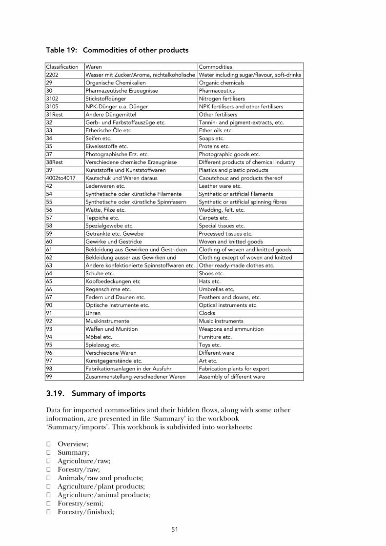
51
Table 19: Commodities of other products Classification Waren Commodities 2202 Wasser mit Zucker/Aroma, nichtalkoholische Water including sugar/flavour, soft-drinks 29 Organische Chemikalien Organic chemicals 30 Pharmazeutische Erzeugnisse Pharmaceutics 3102 Stickstoffdünger Nitrogen fertilisers 3105 NPK-Dünger u.a. Dünger NPK fertilisers and other fertilisers 31Rest Andere Düngemittel Other fertilisers 32 Gerb- und Farbstoffauszüge etc. Tannin- and pigment-extracts, etc. 33 Etherische Öle etc. Ether oils etc. 34 Seifen etc. Soaps etc. 35 Eiweissstoffe etc. Proteins etc. 37 Photographische Erz. etc. Photographic goods etc. 38Rest Verschiedene chemische Erzeugnisse Different products of chemical industry 39 Kunststoffe und Kunststoffwaren Plastics and plastic products 4002to4017 Kautschuk und Waren daraus Caoutchouc and products thereof 42 Lederwaren etc. Leather ware etc. 54 Synthetische oder künstliche Filamente Synthetic or artificial filaments 55 Synthetische oder künstliche Spinnfasern Synthetic or artificial spinning fibres 56 Watte, Filze etc. Wadding, felt, etc. 57 Teppiche etc. Carpets etc. 58 Spezialgewebe etc. Special tissues etc. 59 Getränkte etc. Gewebe Processed tissues etc. 60 Gewirke und Gestricke Woven and knitted goods 61 Bekleidung aus Gewirken und Gestricken Clothing of woven and knitted goods 62 Bekleidung ausser aus Gewirken und Clothing except of woven and knitted 63 Andere konfektionierte Spinnstoffwaren etc. Other ready-made clothes etc. 64 Schuhe etc. Shoes etc. 65 Kopfbedeckungen etc Hats etc. 66 Regenschirme etc. Umbrellas etc. 67 Federn und Daunen etc. Feathers and downs, etc. 90 Optische Instrumente etc. Optical instruments etc. 91 Uhren Clocks 92 Musikinstrumente Music instruments 93 Waffen und Munition Weapons and ammunition 94 Möbel etc. Furniture etc. 95 Spielzeug etc. Toys etc. 96 Verschiedene Waren Different ware 97 Kunstgegenstände etc. Art etc. 98 Fabrikationsanlagen in der Ausfuhr Fabrication plants for export 99 Zusammenstellung verschiedener Waren Assembly of different ware
3.19. Summary of imports
Data for imported commodities and their hidden flows, along with some other information, are presented in file ‘Summary’ in the workbook ‘Summary/imports’. This workbook is subdivided into worksheets: Overview; Summary; Agriculture/raw; Forestry/raw; Animals/raw and products; Agriculture/plant products; Agriculture/animal products; Forestry/semi; Forestry/finished;

52
Biotic/products; Fossils/raw; Metals/raw; Minerals/raw; Fossils/semi; Metals/semi; Minerals/semi; Metals/finished; Minerals/finished; Abiotic products; Other products; Coefficients; Luxury goods. The first worksheet contains data of EU imports from 1988 to 1997 in tonnes, subdivided into individual chapters 1 to 99 of the foreign trade classification system. Each of these chapters indicates in which worksheets (3 to 20) the commodities are classified. Furthermore, the sum of individual commodities in worksheets 3 to 20 belonging to one chapter is compared with the total sum of imports of this chapter to ensure consistency of the basic data. The second worksheet combines the sum values of worksheets 2 to 20 in terms of used and unused material flows. These summary tables are transferred by automatic link to the workbook ‘TMR data summary’. In the ‘Summary’ worksheet, further aggregations of the 18 commodity classes of imports are made with respect to: energy imported; metals imported; minerals imported; biomass imported; erosion; other imports. Minerals are further differentiated by: raw materials: construction minerals; raw materials: industrial minerals; semi-manufactured products: construction minerals; semi-manufactured products: industrial minerals; finished products: construction minerals; finished products: industrial minerals. Another aggregation classifies imports by: raw materials; semi manufactures; finished products; products (other). And yet another aggregation classifies imports by: biotic; abiotic; undefined.

53
Finally, another aggregation classifies imports by: used; unused. Also in worksheet ‘Summary’, all the import data described before, which were in absolute quantities, i.e. tonnes, are expressed in tonnes per capita. Worksheets 3 to 20 in workbook ‘Summary imports’ contain the data of used and unused material flows as described before in chapters 3.1. to 3.18. Where country-specific databases are available to account for hidden flows, the cells containing the classification numbers of the respective commodities are marked in green (in column A). Worksheets 3 to 20 further contain tables of total material inputs (used plus unused material flows) and tables with the ratios of unused to used inputs. Furthermore, worksheets 3 to 20 contain the reference classification numbers according to the EGW classification distinguishing the following four major groups (see also description at the beginning of chapter 3): nutrition industry; commercial industry: raw materials; commercial industry: semi-manufactured products; commercial industry: finished products (with further breakdown into pre-
manufactured and final products). Some specific features of worksheets 3 to 20 are: Worksheet 3 ‘Agriculture/raw’ also presents data of land use for imported commodities in 1 000 hectares, and the specific land use in m2 per kg. Worksheet 6 ‘Agriculture/plant products’ contains an extra aggregation of foodstuffs. Worksheet 7 ‘Agriculture/animal products’ contains an extra aggregation of foodstuffs. Worksheet 12 ‘Metals/raw’ shows some comparisons with global data in terms of (further comparisons are performed in worksheet 22 ‘Luxury goods’): Gold content of extracted ores, among which EU-15:
• EU-15 extraction % of global; • EU-15 import % of global.
Global reserves of gold in central banks, among which EU-15:
• EU-15 reserves % of global. Silver content of extracted ores, among which EU-15:
• EU-15 extraction % of global; • EU-15 Import % of global.
Worksheet 13, ‘Minerals/raw’, contains a subdivision of construction minerals and industrial minerals. Worksheet 16, ‘Minerals/semi’, contains a subdivision of construction minerals and industrial minerals.

54
Worksheet 18, ‘Minerals/finished’, contains a subdivision of construction minerals and industrial minerals. Worksheet 19, ‘Abiotic products’, contains an extra aggregation of chemicals. Worksheet 20, ‘Other products’, contains an extra aggregation of chemicals. Worksheet 21, ‘Coefficients’, combines all the hidden flow coefficients of worksheets 3 to 20 in one table. Worksheet 22, ‘Luxury goods’, combines data of used and unused material flows as well as import values (in 1 000 ECU) of the commodities: 261610: silver ores; 261690: precious metal ores; silver; gold; platinum; precious metals waste/scrap; silver plated ware etc.; gold plated ware etc.; platinum plated ware etc;. jewellery of precious metals etc.; gold- and silver-smith goods; goods of precious metals; fantasy jewellery; coins etc.; diamonds, raw; 710310: precious stones, raw; dust/powder of diamonds/precious stones; pearls, real or cultivated; 710229: diamonds, manufactures; 710239: diamonds, manufactures; 710391: rubies etc., manufactured; 710399: other precious stones, manufactured; goods of pearls, precious stones, etc. Luxury goods are further listed by import prices (ecu per kg) in comparison with: gold, 1000/1000, ingots, London; silver, 999/1000, ingots, New York; iron ore, ca. 64.5 % Fe, Brazil, cif Europe; aluminium, min. 99.7 % al, ingots, storehouse, London; tin, MB free market, min. 99.85 % Sn, London; 261690: (7 tonnes) from Finland to EU(UK); 261690: imports to Germany: total; 261690: imports to Germany: from Sweden; 261690: imports to Germany: from South Africa; 261690: imports to Germany: from other unspecified.

55
Average 1989 prices for PGM and by-products in South Africa (BOM, 1993, p. 23): Co-products: platinum; palladium; rhodium; gold. By-products: cobalt; copper; iridium; nickel; osmium; ruthenium. Imports of luxury goods by EU-15 are further set in relation to global production or supply of: gold content of extracted ores (excluding EU-15); silver content of extracted ores (excluding EU-15); world supply of platinum (excluding recycling); world supply of palladium (excluding recycling); world supply of rhodium (excluding recycling); world supply of other PGM; world supply of total PGM (excluding recycling).

56
4. General data
General data usually set in relation to material flows (Adriaanse et al., 1997) are the population size (capita) and the gross domestic product of economies (GDP). These data for the EU are organised under the file ‘General’ in the worksheets: GDP 1985–97; Population 1985–98. GDP data were taken from Eurostat statistics and expressed in 1985 constant prices. Data from 1993 to 1997 are also given in current prices. Data for 1995 are also given in purchasing power parity (PPP) units as well as the breakdown by EU Member States for conversion of PPP to ecu and USD. Population data were taken from Eurostat statistics.

57
5. TMR data summary
As already mentioned many times, at the points where automatic links of intermediate results are installed, workbook ‘TMR data summary’ under the file ‘Summary’ combines data from the accounting of domestic and foreign flows, and general data, for the calculation, analysis and comparison of TMR of EU-15 with other countries. The workbook ‘TMR data summary’ is subdivided into the following worksheets: Domestic/materials/EU-15; Domestic/materials/EU-12; Domestic/countries; Imports/materials; DMI/EU-15; TMR/EU-12, 1988–94; EU-15, 1995–97; TMR/EU-15, 95; Comparison/FIN, PL, D; Agricultural land use. Worksheet ‘Domestic/materials/EU-15’ takes up the intermediate results for domestic material inputs in EU-15 from 1985 to 1997, divided by used and unused, and aggregates them in the following categories: energy domestic; ores domestic; minerals domestic; excavation domestic; agricultural harvest by statistics; agricultural harvest of additional biomass; fodder plants, additional; erosion; roundwood; fish catch; hunting. Worksheet ‘Domestic/materials/EU-12’ does the same for domestic material inputs in EU-12 from 1985 to 1994. Worksheet ‘Domestic/countries’ presents the intermediate results for domestic material flows from 1985 to 1997, with the material categories listed above, and disaggregated into the 15 individual Member States of the EU. This worksheet also includes the general data for population and GDP. Worksheet ‘Imports/materials’ takes up the intermediate results for imported material flows from 1988 to 1997 from the worksheet ‘Summary’ of the workbook ‘Summary imports’ (see also 3.19.). Worksheet ‘DMI/EU15’ presents the totals of used domestic extractions by EU Member States from 1985 to 1997 (from worksheet ‘Domestic/countries’), and the total of used imported material flows by Member States from 1988 to 1997. Domestic used materials and imports sum up to DMI which is also expressed per capita and per unit GDP.

58
Worksheet ‘TMR/EU-12, 1988-94; EU-15, 1995–97’ summarises the material flow results described above with the following aggregates: Domestic DMI; Domestic HF; Foreign DMI; Foreign HF; DMI; HF; TMI (DMI plus Domestic HF); TMR domestic; TMR foreign; TMR. TMR is further disaggregated by the material groups: fossil fuels; metals; minerals; excavation; biomass; erosion; other (imports). Worksheet ‘EU-15, 1995’ contains a comparison of these TMR material groups on the per capita level of the EU with data from Finland (1995), Germany (1995), Japan (1994), Netherlands (1993), Poland (1995) and the United States (1994). Other comparisons with these countries are made for TMR in relation to their GDPs. A more detailed comparison of EU-15 data with data for Finland, Poland and Germany is made in the worksheet ‘Comparison/FIN, PL, D’. Worksheet ‘Agricultural land use’ combines data of agricultural land use (in 1 000 hectares and in ha per capita) for domestic land (arable land, permanent crops and permanent pastures which sum up to total domestic agricultural land), and for land use due to imported agricultural raw materials.
Contact
Stefan Bringezu Helmut Schütz Wuppertal Institute Doeppersberg 19 42103 Wuppertal, Germany E-mail: [email protected] E-mail: [email protected]

59
6. References
Adriaanse, A., Bringezu, S., Hammond, A., Moriguchi, Y., Rodenburg, E., Rogich, D., Schütz, H. (1997), Resource flows: the material basis of industrial economies. World Resources Institute, Washington.
Adriaanse, A., Bringezu, S., Hammond, A., Moriguchi, Y., Rodenburg, E., Rogich, D., Schütz, H. (1998), ‘Stoffströme: Die materielle Basis von Industriegesellschaften’, Wuppertal Texte, Birkhäuser Verlag, Berlin.
AG Energiebilanzen (working group on energy balances), Energiebilanzen der Bundesrepublik Deutschland (Energy balances of the Federal Republic of Germany), Verlags- und Wirtschaftsgesellschaft der Elektrizitätswerke mbH, Frankfurt/Main, annual publications.
Ayres, R. U., Ayres, L. W. (1996), ‘Industrial ecology: towards closing the materials cycle’, Edward Elgar, Cheltenham, UK, Chapter 4, Copper, cobalt, silver and arsenic, pp.51–68.
BGR (Bundesanstalt für Geowissenschaften und Rohstoffe, German Federal Institution of Geosciences and Raw Materials) (1998), Stoffmengenflüsse und Energiebedarf bei der Gewinnung ausgewählter mineralischer Rohstoffe (Materials quantitative flows and energy requirement for the extraction of selected mineral raw materials), in German, Hannover, Germany.
BOM (Bureau of mines, Information Circular) (1983), Aluminium availability —market economy countries, United States Department of the Interior, IC 8917, Washington DC, United States.
BOM (Bureau of mines, Information Circular) (1984), Nickel availability —market economy countries, United States Department of the Interior, IC 8995, Washington DC, United States.
BOM (Bureau of mines, Information Circular) (1985), Molybdenum availability —market economy countries, United States Department of the Interior, IC 9044, Washington DC, United States.
BOM (Bureau of mines, Information Circular) (1985), Tungsten availability —market economy countries, United States Department of the Interior, IC 9025, Washington DC, United States.
BOM (Bureau of mines, Information Circular) (1986), Gold availability —world, United States Department of the Interior, IC 9070, Washington DC, United States.
BOM (Bureau of mines, Information Circular) (1986), Primary silver availability —market economy countries, United States Department of the Interior, IC 9090, Washington DC, United States.
BOM (Bureau of mines, Information Circular) (1986), Tin availability —market economy countries, United States Department of the Interior, IC 9086, Washington DC, United States.
BOM (Bureau of mines, Information Circular) (1986), Titanium minerals availability —market economy countries, United States Department of the Interior, IC 9061, Washington DC, United States.
BOM (Bureau of mines, Information Circular) (1987), Iron ore availability —market economy countries, United States Department of the Interior, IC 9128, Washington DC, United States.
BOM (Bureau of mines, Information Circular) (1992), Manganese availability —market economy countries: 1980’s perspective, United States Department of the Interior, IC 9327, Washington DC, United States.

60
BOM (Bureau of mines, Information Circular) (1992), The availability of primary copper in market economy countries, United States Department of the Interior, IC 9310, Washington DC, United States.
BOM (Bureau of mines, Information Circular) (1993), Availability of platinum and platinum-group metals, United States Department of the Interior, IC 9338, Washington DC, United States.
BOM (Bureau of mines, Information Circular) (1993), Chromium availability in market economy countries and network flow model analysis of world chromium supply, United States Department of the Interior, IC 9337, Washington DC, United States.
BOM (Bureau Of Mines, Information Circular) (1993), The availability of primary lead and zinc in market economy countries, United States Department of the Interior, IC 9369, Washington DC, United States.
Bringezu, S. (2000), Ressourcennutzung in Wirtschaftsräumen. Stoffstromanalysen für eine nachhaltige Raumentwicklung, Springer Verlag.
Douglas, I., and Lawson, N. (1997), ‘An earth science approach to material flows generated by urbanisation and mining’, in Bringezu, S. et al. (Eds) (1997), Regional and national material flow accounting: from paradigm to practice of sustainability, Proceedings of the ConAccount workshop, 21–23 January 1997, pp. 108–118.
European Minerals Yearbook (EMY), 2nd Edition (1998), available on the DGIII web site (http://europa.eu.int./comm/dg03/publicat/emy).
Eurostat on CD-ROM (© ECSC-EC-EAEC, 1998), Intra- and extra-EU trade.
FAO (Food and Agriculture Organisation of the United Nations, Rome) web site (http://apps.fao.org).
Federal Statistical Office Germany — FSOG, Environmental economic accounting — material- and energy-flow accounting, biannual series 19, part 5, Metzler-Poeschel, Stuttgart.
Federal Statistical Office Germany — FSOG (1999), Gegenüberstellung der Warengruppen und -untergruppen der Ernährungswirtschaft und der Gewerblichen Wirtschaft — EGW und der Warennummern des Warenverzeichnisses für die Aussenhandelsstatistik — WA (Comparative statement of the commodities of the nutrition industry and the commercial industry and the commodity register for foreign trade statistics), in German, document EGW/WA.
Federal Statistical Office Germany — FSOG, Production statistics, annual series 4, part 3.1, Metzler-Poeschel, Stuttgart.
Federal Statistical Office Germany — FSOG, Statistical yearbook for foreign countries, annual publication, Metzler-Poeschel, Stuttgart.
German Federal Institution of Geosciences and Raw Materials (Bundesanstalt für Geowissenschaften und Rohstoffe — BGR), annual reports on the raw materials situation (Jahresberichte zur Rohstoffsituation), in German, Hannover, Germany.
Gocht, W. (Hrsg.), 1985, Handbuch der Metallmärkte (handbook of metal markets), in German, Springer-Verlag, Berlin.
Juutinen, A. and Mäenpää, I., 1999, Time Series for the total material requirement of Finnish economy — Summary, Eco-efficient Finland project, Interim report of 15 August 1999, University of Oulu, Thule Institute (http://thule.oulu.fi/ecoef).
Klinnert, C., (1993), Erfassung von statistischem Datenmaterial über mineralische Rohstoffe (Acquisition of statistical data on mineral raw materials), Bericht an die Abteilung Stoffströme und Strukturwandel des Wuppertal-Institut für Klima, Umwelt und Energie, in German, unveröffentlicht (unpublished).

61
Krauss, H., Saam, H. G., Scjmidt, H. W., Phosphate — Summary report.
Liedtke, C., Merten, T., Kuhndt, M., Baku, B. (1995), ‘Materialintensitäten von Grund-, Werk- und Baustoffen (3) — Die Stahlveredler — (Ferro)-Chrom und (Ferro)-Nickel’, Wuppertal Papers, 38, in German.
Manstein, C. (1995), Quantifizierung und Zurechnung anthropogener Stoffströme im Energiebereich, Diplomarbeit, Bergische Universität — Gesamthochschule Wuppertal, in German.
Merten, T., Liedtke, C., Schmidt-Bleek, F., (1995), ‘Materialintensitäten von Grund-, Werk- und Baustoffen (1) — Die Werkstoffe Beton und Stahl’, Wuppertal Papers, 27, in German.
Mining authorities of the Länder (Germany), Federal Ministry for Economy and Mining Authorities of the Länder, Mining in the Federal Republic of Germany, mining industry and statistics, Trans Tech Publications, annual statistics, in German.
Renner, H., and Johns, M. W. (1989), ‘Gold, gold alloys, and gold compounds’, in Elvers, B. et al. (eds.), Ullmann’s Encyclopedia of Industrial Chemistry, Vol. A12, pp. 499-533, VCH Verlagsgesellschaft mbH, Weinheim, Germany.
Rohn, H., Manstein, C., Liedtke, C. (1995), ‘Materialintensitäten von Grund-, Werk- und Baustoffen (2) — Der Werkstoff Aluminium — Materialintensität von Getränkedosen’, Wuppertal Papers, 37, Wuppertal Institute, in German.
Schmidt-Bleek, F., S. Bringezu, F. Hinterberger, C. Liedtke, J. Spangenberg, H. Stiller, M.J. Welfens, (1998), ‘MAIA — Einführung in die Material-Intensitäts-Analyse nach dem MIPS-Konzept’, Wuppertal Texte, Birkhäuser Verlag, Basel.
Schütz, H. (1997), ‘MFA Germany: Methods, empirical results and trade issues’, in Bringezu, S. et al. (Eds.) (1997), Regional and national material flow accounting: from paradigm to practice of sustainability, Proceedings of the ConAccount Workshop, 21–23 January 1997, pp. 173–177.
Schütz, H., Bringezu, S., (1998), Technical Documentation prepared by the Wuppertal Institute, Division for Material Flows and Structural Change, Economy-wide Material Flow Accounting (MFA),. MFA Workshop, 2–5 June 1998, Wiesbaden.
UN Industrial, (Commodity) Statistics Yearbooks, United Nations, New York.
Unctad (United Nations Conference on Trade and Development), Commodity Yearbook, United Nations, New York and Geneva.
Wilmoth, R. C., Hubbard, S. J., Burckle, J. O., and Martin, J. F. (1991), ‘I.2 production and processing of metals: their disposal and future risks’, in Merian, E. (ed.), Metals and their compounds in the environment, VCH Verlagsgesellschaft mbH, Weinheim (FRG), pp. 19–65.
World Energy Council, World energy statistics.
Wuppertal Institute, Department of Material Flows and Structural Change, ‘Database on material input coefficients’ (Internet: http://www.wupperinst.org/Projekte/mipsonline/download — document: MI-Werte.pdf).
Young, J. E. (1993), Umweltproblem Bergbau, Worldwatch Paper, Band 5, Wochenschau Verlag, Schwalbach/Ts.