total factor productivity estimates for a sample of...

Total Factor Productivity Estimates for a

Sample of European Regions: A Panel

Cointegration Approach

Maria Gabriela Ladu Department of Economics

University of Essex

October 2008

Abstract

This paper looks at the economic performance of the European Regions economies

and compute the total factor productivity using a panel cointegration approach.

The main idea behind this choice is that, �rst of all, this approach allows to di-

rectly estimate di¤erences across economies in the production function and also to

test for the presence of scale economies and market imperfections. Furthermore,

the panel cointegration approach takes non-stationarity issues into account. In

fact, non-stationarity issues on series have been often overlooked when the panel

approach has been used. This paper investigates the stochastic properties of the

regional time series using unit root tests and cointegration tests to guard against

spurious regression problem and to detect long-run relationships. To ignore the

presence of unit roots at best leads to missing important information about the

processes generating the data, and at worst leads to nonsensical results. If unit

roots are present (and the evidence suggests that they generally are) then appro-

priate modelling procedures have to be used. The appropriate modelling here is

cointegration.

0.1 Introduction

A common feature of many empirical studies on international comparison of Total

Factor Productivity (TFP) has been the assumption of identical aggregate pro-

duction function for all countries. However, the empirical evidence suggests that

the production function may actually di¤er across countries but attempts at al-

lowing for such di¤erences have been limited by the fact that most of these studies

have been conducted in the framework of single cross-country regressions. In this

framework it is econometrically di¢ cult to allow for di¤erences in the production

function as these are not easily measurable.

Solow (1956) develops a production function in which output growth is a func-

tion of capital, labour, and knowledge or technology. Technology is Harrod neutral

and it is assumed to be exogenous and homogenous across countries. Economists

use the growth accounting approach to test the neoclassical growth model, and to

evaluate the e¤ect of physical capital accumulation on output growth.

The growth accounting approach provides a breakdown of observed economic

growth into components associated with changes in factor inputs and a residual

that re�ects technological progress and other elements. The basic of growth ac-

counting were presented in Solow (1957).1

1Di¤erentiation of the neoclassical production function Y = F (A;K;L) with respect to timeyields:

_Y

Y= g + (

FKK

Y) � ( _K=K) + (FLL

Y) � ( _L=L) (1)

where FKand F

Lare the factor marginal products and g is the technological progress, given by:

g � (FAAY

) � (_A

A) (2)

g =_Y

Y� FKK

Y) � ( _K=K)� (FLL

Y) � ( _L=L) (3)

i

The results of the early growth accounting exercises raise questions about the

large unexplained residual in Solow-model calculations. The neoclassical model

emphasizes the role of factor accumulation, neglecting di¤erences in productivity

growth and technological change captured by the residual. By de�ning capital to

include physical and human capital, Mankiw (1995) �nds that the results more

closely resemble the theoretical prediction of the neoclassical model. The works of

Barro and Sala-i-Martin (1995), Mankiw, Romer and Weil (1992) follow a similar

perspective.

Easterly and Levine (2001) suggest that growth economists should focus on

TFP and its determinants rather than factor accumulation. They point out that

much of the empirical evidence accumulated to date indicates that factor accu-

mulation explains only a portion of the observed cross-country growth. Solow

(1956) himself �nds that income growth is explained only in little part by capital

accumulation while the rest is explained by productivity growth. Easterly and

Levine (2001) also observe that there exists a tendency of production factors to

move to the same places, causing a concentration of economic activity. In such

circumstances, to apply the neoclassical model with homogenous technology is not

appropriate.

Endogenous growth theory, starting from Romer (1986) and Lucas (1988), de-

parts from the standard neoclassical theory and considers the technological change

as endogenous. The theory focuses on explaining the Solow residual.

Going back to the growth accounting approach, it is important to point out

that it presents two major shortcomings: �rst of all, a key assumption is that

If the technological progress is Hicks neutral then F (A;K;L) = A � ~F (K;L) and g = _AA . The

technological change can be calculated as a residual (Solow residual) from (1).

ii

prices coincide with social marginal products. If this assumption is violated, then

the estimated Solow residual deviates from the true contribution of technological

change to economic growth. Moreover, this approach ignores consideration on

market power and returns to scale.

Hall and Jones (1996, 1997) suggest the cross-section growth accounting ap-

proach to TFP level comparisons and they follow Solow (1957) to arrive at the

standard growth accounting equation. The di¤erence with respect to Solow is that

while in Solow (1957) di¤erentiation is conducted in the direction of time t, Hall

and Jones propose to apply the procedure in the cross-sectional direction, i.e. in

the direction of i. But this poses a problem because the movement on i depends on

the particular way the countries are ordered. Hall and Jones order the countries

on the basis of an index that is a linear combination of the individual country�s

physical and human capital per unit of labor and its value of �, the share of phys-

ical capital in income. In order to get the country speci�c �, the authors make

the assumption that price of capital (r) is the same across countries.

The cross-section growth accounting approach presents several advantages.

First, it does not require any speci�c form of aggregate production function. Only

constant returns to scale and di¤erentiability are required to arrive at the growth

accounting equation. Second, it allows factor income share parameters to be dif-

ferent across countries. However, the cross-section growth accounting approach

has some weaknesses too. First, it requires prior ordering of countries and TFP

measurement may be sensitive to the ordering chosen. Second, TFP indices are

also sensitive to inclusion or exclusion of countries. Third, computation of �i is

made on the basis of the assumption of a uniform rate of return across countries.

Finally, using capital stock data and accounting for human capital in cross-country

iii

TFP comparison, it is possible to pick up some noise.

The panel approach to international TFP comparisons arose directly from re-

cent attempts at better explaining cross-country growth regularities. Islam (1995)

takes the work of Mankiw, Romer and Weil (1992) as his starting point and ex-

amines how the results change with the adoption of the panel data approach. The

main usefulness of the panel approach with respect to the single cross-country

regressions lies in its ability to allow for di¤erences in the aggregate production

function across economies. This leads to results that are signi�cantly di¤erent

from those obtained from single cross-country regressions. The panel approach

makes it possible to allow for di¤erences in the aggregate production function in

the form of unobservable individual "country e¤ects". To the extent to which the

"country e¤ects" (intercepts) are correlated with the regressors, the conventional

cross-section estimates of Mankiw, Romer and Weil (1992) are biased. Harrigan

(1995) shows that there are systematic di¤erences across countries in industry out-

put. One possible explanation for this result is that technology is not the same

across countries. This hypothesis has gained great attention from international

economists: Tre�er (1993, 1995), Dollar and Wol¤ (1993) and Harrigan (1997a).

More recently, Harrigan (1999) compute TFP for eleven OECD countries in the

1980s and he �nds large and persistent TFP di¤erences among them.

In comparison with the cross-section growth accounting approach, the panel

regression approach has some advantage. First, it does not require any prior order-

ing of countries. Second, it is not sensitive to inclusion or exclusion of countries.

Third, the approach is �exible to the use of capital stock data or investment data

and to inclusion of human capital. Finally, the econometric estimation can provide

a check for the severity of noise in the relevant data. Of course, the panel approach

iv

also presents some weaknesses: it requires a speci�c form for aggregate produc-

tion function, it imposes homogeneity of factor share parameters and, �nally, it is

subject to certain pitfalls of econometric estimation.2

The aim of this paper is to analyze the economic performance of a sample

of European regions using a panel data approach. The main idea behind this

choice is that this approach allows for di¤erences across countries and regions. In

fact, recent studies (de la Fuente (1995, 1996b) and de la Fuente and Doménech

(2000)) show that total factor productivity (TFP) di¤erences across countries and

regions are substantial and highlight the importance of TFP dynamics as crucial

in the evolution of productivity. Furthermore, the empirical literature shows that

regional disparities are larger when compared to cross-country di¤erences and in

spite of the acceleration of the European integration, disparities has remained

an open issue, especially on economic growth and employment. Therefore, the

existence of large disparities among European regions justi�es the choice of this

chapter to analyze the TFP at regional level instead that at national level. Finally,

it is worth noting the fact that these large di¤erences among regions in Europe

have important implications for the economic policies of the European Union.

Le Gallo and Dall�erba (2006) analyzes the productivity structure of 145 EU

regions according to the concepts of �- and �- convergence, including spatial e¤ects

and a disaggregated analysis at a sectoral level. They detect �- convergence in

aggregate labour productivity and in the service sectors but not in other sectors.

They also estimate �- convergence models and the results show that inequality in

productivity levels between core and peripheral regions persist.

2The cost of econometric analysis is that parameter estimation requires imposing a statisticalmodel on the data (see Harrigan,1999)

v

Marrocu, Paci e Pala (2000) estimate a complete set of long-run production

functions for 20 Italian regions and 17 economic sectors. They �nd that regions

di¤er considerably in the technological knowledge levels. Furthermore they �nd

that the 11 highest levels are those of the northern regions of Italy and the lowest

are those for southern regions.

Boldrin and Canova (2001) study the disparities across the regions of EU 15.

They show that neither convergence nor divergence is taking place within EU and

that most regions are growing at a near uniform growth rate, with some exceptions.

They also show that the evolution of TFP and labour productivity in the poorer

regions are not a¤ected by the amount of funds invested under EU programmes.

Boldrin and Canova argue that most of the observed disparities in regional income

levels derive from the combination of three factors: di¤erences in TFP, di¤erences

in employment levels, and di¤erences in the share of agriculture in regional income.

Paci, Pigliaru and Pugno (2001) study the disparities on productivity growth

and unemployment across European regions, adopting a sectoral perspective, i.e.

by considering the relationship between agriculture, industry and services, and

their role in enhancing growth and absorbing employment. They �nd that regions

that start from a high agricultural share are characterized by higher growth rates

than average; on the contrary regions with low agricultural share are the richest and

grow slowly. Furthermore, they �nd that convergence in aggregate productivity is

strongly associated with out-migration from agriculture.

Here, I use a Cobb-Douglas speci�cation for a sample of 115 European Regions

over the period 1976-2000 and I provide estimates of TFP for each region.

This work also shows, on the basis of speci�c panel tests, that there is empirical

evidence which suggests the presence of unit roots in the series under study. I

vi

apply, then, the panel cointegration test, proposed by Pedroni (1999), to guard

against spurious regression problems.

This paper is organized as follows. Section 0.2 describes the model. Section 0.3

describes the econometric methodology. Section 0.4 presents the empirical results.

Section 0.5 concludes.

0.2 The model

I estimate the parameters of production functions and calculate total factor pro-

ductivity for a sample of European regions from Cobb-Douglas production function

speci�cations:

Yit = AitK�itL

�it (4)

where Yit is the value added in region i at time period t, Kit is the stock of physical

capital, Lit is the amount of labour used in production. Ait is the speci�cation for

Hicks-neutral technology and it introduces a stochastic component into the model.

The knowledge production function for region i at time period t can be de�ned as

follows: in region i at time period t

Ait = eai+ t+"it (5)

where Ait is the level of technology in region i at time t, ai denotes a region speci�c

constant which captures the e¢ ciency in technology production, t is a common

time e¤ect which captures the countrywide or worldwide knowledge accumulation

and "it is a random shock. The common time e¤ect t allows to take account of

vii

cross-regional dependence in the estimation of the regional production function.

Rewriting equation (4) in natural logarithms yields the following:

lnYit = ai + t + � lnKit + � lnLit + "it (6)

The panel model includes a regional speci�c e¤ect ai and a common time e¤ect t.

The parameters � and � are the elasticities of capital and labour with respect to

output, respectively. This paper estimates 6 by using a panel data of 115 European

regions over the period 1976-2000. The list of the regions is given in table (2). The

stock of physical capital is determined by using the Perpetual Inventory Method :

Kt = (1� �)Kt�1 + It�1 (7)

where � is the depreciation rate: it is assumed constant and equal to 8%, which

is consistent with OECD estimates; I is the gross �xed capital formation.3 The

initial value of K is calculate as:

K0 =I0g + �

(8)

where g is the average annual logarithmic growth of investment expenditure and

I0 is investment expenditure in the �rst year for which data on investment are

available.3See Machin and Van Reenen, (1998)

viii

0.3 Econometric methodology

Non-stationarity issues on series have been often overlooked when the panel ap-

proach has been used to estimate production functions. At the best of my knowl-

edge, no attempt has been made to asses the non-stationarity of the series used

on the estimation of production functions for European regions. Because of non-

stationarity problems, �rst step of this work is to investigate the properties of

regional time series for value-added, capital stock and labour. I start applying

the panel unit root test proposed by Im, Pesaran and Shin (2003, IPS hereafter),

while the spurious regression problem is analyzed through the cointegration test

recently proposed by Pedroni (1999).

0.3.1 Panel unit root tests

Over the past decade a number of important panel data set covering di¤erent

countries, regions or industries over long time spans have become available. This

raises the issue of the plausibility of the dynamic homogeneity assumption that

characterizes the traditional analysis of panel data models. The inconsistency of

pooled estimators in dynamic heterogeneous panel models has been demonstrated

by Pesaran and Smith (1995), and Pesaran et al.(1996).

Panel based unit root tests have been advanced by Quah (1990, 1994), Bre-

itung and Meyer (1991), Levin and Lin (1992), Phillips and Moon (1999), Levin,

Lin and Chu (2002) and Im, Pesaran and Shin (2003), among others. Quah (1990,

1994) uses the random �eld methods to analyze a panel with i.i.d. disturbances,

and demonstrates that the Dickey-Fuller test statistic has a standard normal lim-

iting distribution as both cross-section and time series dimensions grow arbitrarily

ix

large. Unfortunately, the random �eld method does not allow for individual spe-

ci�c e¤ects. Breitung and Meyer (1991) approach allows for time speci�c e¤ects

and higher-order serial correlation, but cannot be extended to panel with hetero-

geneous errors. Levin and Lin test allows for heterogeneity only in the intercept

and is based on the following model

�yit = �yi;t�1 + �midmt + uit (9)

i = 1; :::; N ; t = 1; :::T ; m = 1; 2; 3, where dmt contains deterministic variables;

d1t = f0g; d2t = f1g; d3t = f1; tg. The Levin and Lin test requires the strong

condition N=T ! 0 for its asymptotic validity. A revised version of Levin and

Lin�s (1992) earlier work is proposed by Levin, Lin and Chu (2002). The panel-

based unit root test proposed in this paper allows for individual-speci�c intercepts,

the degree of persistence in individual regression error and trend coe¢ cient to vary

freely across individuals. This test is relevant for panels of moderate size. However,

this test has its limitations. First, there are some cases in which contemporaneous

correlations cannot be removed by simply subtracting cross-sectional averages.

Secondly, the assumption that all individuals are identical with respect to the

presence or absence of a unit root is, in some sense, restrictive.

Im, Pesaran and Shin (2003) propose unit root tests for dynamic heterogeneous

panels based on the mean of individual unit root test statistics. In particular they

propose a standardized t-bar test statistic based on the (augmented) Dickey-Fuller

statistics averaged across the groups.

Consider a sample of N cross-section observed over T time periods. IPS sup-

pose that the stochastic process, yit, is generated by the �rst-order autoregressive

x

process:

yit = (1� �i)�i + �iyi;t�1 + �it (10)

i = 1; :::; N , t = 1; :::; T , where initial values, yi0, are given. The null hypothesis

of unit roots �i = 1 can be expressed as

�yit = �i + �iyi;t�1 + �it (11)

where �i = (1��i)�i, �i = �(1��i) and �yit = (yit�yi;t�1). The null hypothesis

of unit roots then becomes

H0 : �i = 0 (12)

for all i, against the alternatives

H1 : �i < 0, i = 1; :::; N1, �i = 0, i = N1 + 1; N2 + 1; :::; N .

This formulation of the alternative hypothesis allows for �i to di¤er across

groups, and is more general than the homogeneous alternative hypothesis, namely

�i = � < 0 for all i, which is implicit in the testing approaches of Quah and

Levin-Lin.

The IPS group-mean t-bar statistic is given by:

t� barNT= N

�1NXi=1

tiTi(pi) (13)

where tiTi is the individual t statistic for time series with di¤erent lag lengths.

xi

0.3.2 Panel cointegration test

Methods for nonstationary panels have been gaining increased acceptance in recent

empirical research. Initial theoretical work on nonstationary panels focused on

testing for unit roots in univariate panels.4 However, many applications involve

multi-variate relationships and a researcher is interested to know whether or not

a particular set of variables is cointegrated. Pedroni (1999) proposes a method to

implement tests for the null of cointegration for the case with multiple regressors.

The tests allow for a considerable heterogeneity among individual members of the

panel.5

Testing for cointegration in heterogeneous panels: the multivariate case

Here I provide a complete description of the test proposed by Pedroni. The �rst

step is to compute the regression residuals from the hypothesized cointegrating

regression. The general case is:

yit = �i + �it+ �1iX1it + �2iX2it + :::+ �MiXMit+ eit (14)

for t = 1; :::; T ; m = 1; :::;M , where T refers to the number of observation over

time, N refers to the number of individual members in the panel, and M refers

to the number of variables. The parameter �i is the �xed e¤ects parameter and

�1i, �2i,..., �Mi are the slope coe¢ cients. Both the �xed e¤ects parameter and

slope coe¢ cients are allowed to vary across individual members. �it represents a

deterministic time trend, which might be included in some applications.

4See for instance, Levin and Lin (1993) and Quah (1994).5Pedroni cointegration tests include heterogeneity in both the long run cointegrating vectors

as well as in the dynamics associated with short run deviations from these one.

xii

To capture disturbances, which may be shared across the di¤erent members of

the panel, common time dummies can be included.

Pedroni derives the asymptotic distributions of seven di¤erent statistics: four

are based on pooling along the within-dimension, and three are based on pooling

along the between-dimension. Pedroni calls the within-dimension based statistics

as panel cointegration statistics, and the between-dimension based statistics as

group mean panel cointegration statistics. The �rst of the panel cointegration sta-

tistics is a type of nonparametric variance ratio statistic. The second is a panel ver-

sion of nonparametric statistic analogous to the Phillips and Perron rho-statistic.

The third statistic is also nonparametric and analogous to the Phillips and Perron

t-statistic. The fourth of the panel cointegration statistics is a parametric statistic

analogous to the augmented Dickey-Fuller t-statistic.

The other three statistics are based on a group mean approach. The �rst

and the second ones are analogous to the Phillips and Perron rho and t-statistic

respectively, while the third one is analogous to the augmented Dickey-Fuller t-

statistic.

Table (1) presents the seven statistics.

Pedroni panel cointegration test computes the seven statistics following a pro-

cedure in steps:

1. Estimate the panel cointegration regression (14) and collect residuals eit;

2. Estimate (14) in di¤erences and collect residuals (�it);

3. Compute the long run variance of �itusing a kernel estimator, such as the

Newey-West (1987) estimator, and calculate L�2

11i;

xiii

Table 1: Panel Cointegration Statistics

Panel Statistics (within)v T

2N

3=2Z�NT� T

2

N3=2(PN

i=1

PT

t=1L�2

11ie2

it�1)�1

� TpNZ�NT�1� T

pN(PN

i=1

PT

t=1L�2

11ie2

it�1)�1PN

i=1

PT

t=1L�2

11i(e

it�1�eit��i)

tnonparametric

ZtNT� (~�2

NT

PN

i=1

PT

t=1L�2

11ie2

it�1)�1=2PN

i=1

PT

t=1L�2

11i(e


t(parametric)

Z�tNT� (~s

2

NT

PN

i=1

PT

t=1L�2

11ie�2

it�1)�1=2PN

i=1

PT

t=1L�2

11ie�

it�1�e

�

it

Group Statistics (between)� TN

�1=2Z�NT�1� TN

�1=2PN

i=1(PT

t=1e2

it�1)�1PT

t=1(e


t(nonparametric)

N�1=2 ~Z

�tNT� N�1=2PN

i=1(�

2

i

PT

t=1e2

it�1)�1=2PT

t=1(e


t(parametric)

N�1=2 ~Z

�tNT� N�1=2PN

i=1(PT

t=1s�2i e

�2

it�1)�1=2PT

t=1e�

it�1�e

�

it

where �i= 1

T

Pki

s=1(1� s

ki+1)PT

t=s+1�it�it�s ;

s2

i� 1

T

PTt=1 �

2

it;

�2

i= s

2

i+ 2�

i;

~�2

NT� 1

N

PN

i=1L�2

11i�2

i;

s�2i � 1

T

PTt=1 �

�2

it;

~s�2

NT� 1

N

PN

i=1s�2i ;

L�2

11i= 1

T

PTt=1 �

2

it+ 2

T

Pki

s=1(1� s

ki+1)PT

t=s+1�it�it�s

and where �it, �

�

itand �

itare obtained from the following regressions:

eit= �

ieit�1

+ uit, e

it= �

ieit�1

+PKi

k=1 ik�e

it�k+ u

�

it,

�yit=PM

m=1bmit�X

mit+ �

it

xiv

4. Use the residuals eitand :

a) compute the non parametric statistics estimating the following regression:

eit= �

ieit�1

+ uit

The residuals (uit) are used to calculate the long run variance, denoted

by �2

i, while s

2

iis the simple variance of u

itand the term �

iis calculated

as �i =12(�

2

i� s2

i);

b) compute the parametric statistics estimating the following regression:

eit= �

ieit�1

+

KiXk=1

ik�e

it�k+ u

�

it

and use the residuals (u�

it) to compute the simple variance s

�2i .

Pedroni (1995, 1997a) shows that each of the seven statistics presented in table

(1) will be distributed as standard normal after an appropriate standardization.

This standardization depends only on the moments of certain Brownian motion

functionals.6 In Pedroni (1999) the moments of the vector of Brownian motion

functionals are computed by Monte Carlo simulation for the case of multiple re-

gressors.

The asymptotic distributions for each of the seven panel and group mean sta-

6A Brownian motion is a continuous-time stochastic process with three important properties.First, it is a Markov process and it means that the probabilty distribution for all future valuesof the process depends only on its current value. Second, the Brownian process has indipen-dent increments. Finally, changes in the process over any �nite interval of time are normallydistributed.

xv

tistics can be expressed in the form

{NT� �

pNp

�! N(0; 1)

where {NTis the standardized form of the statistics as described in table (1), and

the value for � and � are functions of the moments of Brownian motion functionals.

0.3.3 Panel estimation of long-run relationship

The main theme of this chapter is to analyze the economic performance of a sam-

ple of European regions. But it is worth emphasising that only if the cointegration

test provides evidence of long run dynamics in the series, although they are non-

stationary, it is possible to proceed with the analysis. I have in mind a particular

form of normalization among variables (a production function relation) and in this

case, as pointed out by Pedroni, the interest is in knowing whether the variables

are cointegrated, not how many cointegrating vectors exist.

The model I use is a two error component model, with uit = ai+ t+"it, and "it

is assumed homoskedastic. If the assumption fails, the estimates are still consistent

but ine¢ cient. It is possible to investigate about the validity of this assumption

by performing a groupwise likelihood ratio heteroskedasticity test. This test is

performed on the residuals of the model estimated by OLS. The test is chi-square

distributed with N � 1 degrees of freedom, where N is the number of groups in

the sample.

Baltagi and Li (1995) suggest an LM test for serial correlation in �xed e¤ects

models. They propose two versions of the test, depending on the assumption for the

autocorrelation structure, namely AR(1) and MA(1). The test is asymptotically

xvi

distributed as N(0; 1) under the null.

0.4 Data and empirical results

In my analysis I use a panel of 115 European regions over the period 1976-2000

(see table 2). The level of territorial disaggregation provides the maximum dis-

aggregation possible with the data available. This level corresponds to NUTS 2

for Spain, Italy, Greece, France, Austria; NUTS 1 for Belgium, Germany, Nether-

lands, United Kingdom; NUTS 0 for Ireland, Denmark and Luxembourg. Annual

data on value added and labour units are from Cambridge Econometrics dataset.

The stock of capital is determined by using the Perpetual Inventory Method and

is measured at 1995 constant prices, as value added.

There is a great disparity among regions and even across regions of the same

countries. The poorest regions are those from Spain, Greece, southern regions

of Italy and almost all UK regions. The richest ones are Wien, Ile de France,

Hamburg and Bruxelles. The lowest rate of growth of value added is for Sterea

Ellada (Greece. 0; 7%), while the highest one is for Ireland (close to 4%) (see table

3). Extremadura (Spain) shows the lowest level of value added but its growth rate

is high (over 3%). If we look at the employment performance (see table 4) over the

period examined, we will see disparities again among regions and across regions

of the same country. The worst performance is that for Ditiky Ellada (Greece,

�1:89%);the best one is that for Ceuta y Melilla (Spain, 2:55%)

I analyze the time series properties of my data, applying the IPS panel root

test to control for stationarity of the three variables included in the panel used

to estimate the production function. Table 6 reports the results of the test for

xvii

Table 2: The Sample of RegionsRegions

Belg ium - NUTS1

Bruxelles-B russel (Be) Asturias (Es)

V laam s Gewest (Be) Cantabria (Es)

Region Walonne (Be) Pais Vasco (Es)

Denmark - NUTS 0 Navarra (Es)

Germany - NUTS 1 R io ja (Es)

Baden-Wurttemberg (De) Aragon (Es)

Bayern (De) Madrid (Es)

Berlin (De) Castilla -Leon (Es)

Brem en (De) Castilla -la M ancha (Es)

Hamburg (De) Extremadura (Es)

Hessen (De) Cataluna (Es)

N iedersachsen (De) Com . Valenciana (Es)

Nordrhein -Westfa len (De) Baleares (Es)

Rhein land-P falz (De) Andalucia (Es)

Saarland (De) Murcia (Es)

Sch lesw ig-Holstein (De) Ceuta y M elilla (Es)

G reece - NUTS2 Canarias (Es)

Anatolik i M akedonia (G r) France - NUTS 2

Kentrik i M akedonia (G r) Ile de France (Fr)

Dytik i M akedonia (G r) Champagne-Ard (Fr)

Thessalia (G r) P icard ie (Fr)

Ip eiros (G r) Haute-Normandie (Fr)

Ion ia N isia (G r) Centre (Fr)

Dytik i E llada (G r) BassCentre (Fr)e-Normandie (Fr)

Sterea E llada (G r) Bourgogne (Fr)

Pelop onnisos (G r) Nord-Pas de Cala is (Fr)

Attik i (G r) Lorra ine (Fr)

Voreio A igaio (G r) A lsace (Fr)

Notio A igaio (G r) Franche-Comte (Fr)

K riti (G r) Pays de la Loire (Fr)

Spain - NUTS 2 Bretagne (Fr)

Galic ia (Es) Poitou-Charentes (Fr)

Regions

Aquita ine (Fr) Oost-Nederland (N l)

M id i-Pyrenees (Fr) West-Nederland (N l)

L imousin (Fr) Zuid-Nederland (N l)

Rhone-A lp es (Fr) Austria - NUTS 2

Auvergne (Fr) Burgen land (At)

Languedoc-Rouss. (Fr) N iederosterreich (At)

Prov-A lp es-Cote d�Azur (Fr) W ien (At)

Corse (Fr) Karnten (At)

Ireland - NUTS 0 Steiermark (At)

Ita ly - NUTS 2 Oberosterreich (At)

P iemonte (It) Salzburg (At)

Valle d�Aosta (It) T iro l (At)

L iguria (It) Vorarlb erg (At)

Lombard ia (It) United K ingdom - NUTS 1

Trentino-A lto Adige (It) North East (GB)

Veneto (It) North West (GB)

Fr.-Venezia G iu lia (It) Yorksh ire and the Humb (GB)

Em ilia-Romagna (It) East M id lands (GB)

Toscana (It) West M id lands (GB)

Umbria (It) Eastern (GB)

Marche (It) London (GB)

Lazio (It) South East (GB)

Abruzzo (It) South West (GB)

Molise (It) Wales (GB)

Campania (It) Scotland (GB)

Puglia (It) Northern Ireland (GB)

Basilicata (It)

Calabria (It)

S icilia (It)

Sardegna (It)

Luxembourg - NUTS - 0

Netherlands - NUTS 2

Noord-Nederland (N l)

xviii

Table 3: Gross Value Added growth rateRegions gva-g

Bruxelles-B ruxelles (Be) 1.79

V laam s Gewest (Be) 2.31

Region Walonne (Be) 1.48

Denmark - NUTS 0 1.66

Baden-Wurttemberg (De) 1.82

Bayern (De) 2.39

Berlin (De) 0.70

Brem en (De) 1.65

Hamburg (De) 1.90

Hessen (De) 2.28

N iedersachsen (De) 1.68

Nordrhein -Westfa len (De) 1.35

Rhein land-P falz (De) 1.38

Saarland (De) 1.64

Sch lesw ig-Holstein (De) 1.57

Anatolik i M akedonia (G r) 1.74

Kentrik i M akedonia (G r) 1.20

Dytik i M akedonia (G r) 0.97

Thessalia (G r) 1.25

Ip eiros (G r) 0.83

Ion ia N isia (G r) 1.72

Dytik i E llada (G r) 0.86

Sterea E llada (G r) 0.44

Pelop onnisos (G r) 0.73

Attik i (G r) 0.69

Voreio A igaio (G r) 1.75

Notio A igaio (G r) 2.67

Kriti (G r) 2.43

Galic ia (Es) 2.41

Asturias (Es) 2.06

Cantabria (Es) 2.19

Pais Vasco (Es) 2.45

Navarra (Es) 2.57

Regions gva-g

R io ja (Es) 2.47

Aragon (Es) 3.03

Madrid (Es) 3.25

Castilla -Leon (Es) 2.51

Castilla -la Mancha (Es) 2.71

Extremadura (Es) 3.21

Cataluna (Es) 3.12

Com . Valenciana (Es) 2.43

Baleares (Es) 3.19

Andalucia (Es) 2.47

Murcia (Es) 2.21

Ceuta y M elilla (Es) 2.94

Canarias (Es) 3.59

Ile de France (Fr) 2.02

Champagne-Ard (Fr) 1.56

P icard ie (Fr) 1.24

Haute-Normandie (Fr) 1.18

Centre (Fr) 1.77

BassCentre (Fr)e-Normandie (Fr) 2.11

Bourgogne (Fr) 1.82

Nord-Pas de Cala is (Fr) 1 .37

Lorraine (Fr) 1.10

A lsace (Fr) 1.67

Franche-Comte (Fr) 1.38

Pays de la Loire (Fr) 1.93

Bretagne (Fr) 1.93

Poitou-Charentes (Fr) 1.72

Aquita ine (Fr) 1.77

M id i-Pyrenees (Fr) 2.23

L imousin (Fr) 2.12

Rhone-A lp es (Fr) 1.75

Auvergne (Fr) 1.88

Languedoc-Rouss. (Fr) 1 .83

Regions gva-g

Prov-A lp es (Fr) 1.41

Corse (Fr) 1.73

Ireland 4.36

P iemonte (It) 1 .73

Valle d�Aosta (It) 1 .50

L iguria (It) 2 .45

Lombard ia (It) 1 .93

Trentino-AA (It) 2 .29

Veneto (It) 2 .39

Fr.-V G iu lia (It) 2 .15

Em ilia-R (It) 1 .91

Toscana (It) 1 .91

Umbria (It) 1 .53

Marche (It) 1 .66

Lazio (It) 2 .22

Abruzzo (It) 1 .84

Molise (It 2 .18

Campania (It) 1 .81

Puglia (It) 1 .60

Basilicata (It) 2 .18

Calabria (It) 2 .08

S icilia (It) 1 .91

Sardegna (It) 1 .96

Luxembourg 3.25

Noord-Ned (N l) 0 .78

Oost-Ned (N l) 2 .06

West-Ned (N l) 2 .18

Zuid-Nederland (N l) 2 .60

Burgen land (At) 3.36

N iederosterreich (At) 3.26

W ien (At) 3.01

Karnten (At) 2.79

Steiermark (At) 2.63

Oberosterreich (At) 2.75

Regions gva-g

Salzburg (At) 2.60

T iro l (At) 2.27

Vorarlb erg (At) 2.42

North East (GB) 1.28

North West (GB) 1.73

Yorksh ire (GB) 1.95

East M id l (GB) 2.04

West M id l (GB) 2.01

Eastern (GB) 2.29

London (GB) 2.27

South East (GB) 2.60

South West (GB) 2.07

Wales (GB) 2.03

Scotland(GB) 2.07

Northern Ir (GB) 1.98

xix

Table 4: Employment growth rateRegions emp-g

Bruxelles-B ruxelles (Be) -0 .41


Region Walonne (Be) -0 .14



Bayern (De) 0.80

Berlin (De) 0.62

Brem en (De) -0 .06

Hamburg (De) 0.28

Hessen (De) 0.60




Saarland (De) 0.34




Dytik i M akedonia (G r) 0

Thessalia (G r) -0 .45

Ip eiros (G r) -1 .62


Dytik i E llada (G r) -1 .89

Sterea E llada (G r) -1 .33

Pelop onnisos (G r) -0 .26

Attik i (G r) 1.68

Voreio A igaio (G r) -0 .96


Kriti (G r) 0.99

Galic ia (Es) -0 .20

Asturias (Es) -0 .53

Cantabria (Es) -0 .23


Navarra (Es) 0.68

Regions emp-g

R io ja (Es) 0.33

Aragon (Es) 0.41

Madrid (Es) 1.53

Castilla -Leon (Es) -0 .07

Castilla -la M ancha (Es) 0.61


Cataluna (Es) 0.90


Baleares (Es) 1.46

Andalucia (Es) 0.73

Murcia (Es) 1.40


Canarias (Es) 1.36


Champagne-Ard (Fr) -0 .19

P icard ie (Fr) -0 .01

Haute-Normandie (Fr) -0 .01

Centre (Fr) 0.12


Bourgogne (Fr) -0 .19

Nord-Pas de Cala is (Fr) -0 .10

Lorraine (Fr) -0 .25

A lsace (Fr) 0.55

Franche-Comte (Fr) -0 .13


Bretagne (Fr) 0.40

Poitou-Charentes (Fr) -0 .12



L imousin (Fr) -0 .46


Auvergne (Fr) -0 .42


Regions emp-g


Corse (Fr) 0.81

Ireland 1.65



L iguria (It) -0 .07



Veneto (It) 0 .87



Toscana (It) 0 .29

Umbria (It) 0 .12

Marche (It) 0 .16

Lazio (It) 0 .82

Abruzzo (It) 0 .22

Molise (It -0 .51

Campania (It) 0 .04

Puglia (It) -0 .57

Basilicata (It) -0 .31

Calabria (It) -0 .05

S icilia (It) 0 .33

Sardegna (It) 0 .49

Luxembourg 1.98







W ien (At) 0

Karnten (At) 0.52



Regions emp-g

Salzburg (At) 0.92

T iro l (At) 1.06


North East (GB) -0.49

North West (GB) -0.13




Eastern (GB) 0.86

London (GB) 0.16



Wales (GB) 0

Scotland(GB) -0.07


xx

Table 5: Capital growth rateRegions K -g






Bayern (De) 3.15

Berlin (De) 2.02

Brem en (De) 1.72

Hamburg (De) 1.56

Hessen (De) 3.08




Saarland (De) 1.88






Ip eiros (G r) 3.96





Attik i (G r) 1.84



Kriti (G r) 5.03

Galic ia (Es) 0.12

Asturias (Es) -0 .57

Cantabria (Es) 0.15

Pais Vasco (Es) -0 .11

Navarra (Es) 0.70

Regions K -g

R io ja (Es) 0.65

Aragon (Es) 0.73

Madrid (Es) 1.74




Cataluna (Es) 1.17


Baleares (Es) 2.28

Andalucia (Es) 0.98

Murcia (Es) 0.73

Ceuta y M elilla (Es) -1 .61

Canarias (Es) 2.58





Centre (Fr) 2.79


Bourgogne (Fr) 2.54


Lorraine (Fr) 1.23

A lsace (Fr) 2.33



Bretagne (Fr) 1.85




L imousin (Fr) 2.28


Auvergne (Fr) 2.02


Regions K -g


Corse (Fr) 2.62

Ireland 5.03



L iguria (It) 0 .42



Veneto (It) 1 .04



Toscana (It) 0 .53

Umbria (It) 0 .28

Marche (It) 0 .39

Lazio (It) 1 .00

Abruzzo (It) 0 .41

Molise (It 0 .93

Campania (It) 0 .69

Puglia (It) 0 .40


Calabria (It) 0 .63

S icilia (It) 0 .72

Sardegna (It) 0 .81

Luxembourg -0 .20


Oost-Ned (N l) -0 .98

West-Ned (N l) -1 .34

Zuid-Nederland (N l) -0 .51



W ien (At) 2.70

Karnten (At) 0.92



Regions K -g

Salzburg (At) 3.44

T iro l (At) 2.70







Eastern (GB) 2.87

London (GB) 1.14



Wales (GB) 2.57

Scotland(GB) 2.14


xxi

Table 6: Panel Unit Root TestVariables t� bar t� bar�

Y 0:95(0:83)

�1:20(0:12)

K 0:43(0:67)

1:45(0:93)

L 0:27(0:61)

�4:07(0:00)

�Y �8:87(0:00)

�4:82(0:00)

�K �2:43(0:01)

�1:77(0:04)

�L �8:48(0:00)

�2:63(0:00)

Notes: p-values are in brackets. All variables are in logs.

The test statistics are asymptotically distributed as N(0,1) under

the null hypothesis of non-stationarity.

the logarithm of value added (Y ), capital stock (K) and labour (L). The test is

performed both on levels and �rst di¤erences (�Y;�K;�L) of the variables. The

null hypothesis refers to non-stationarity behavior of the time series. Under the

null of non-stationarity. the test is distributed as N(0; 1), so that large negative

numbers indicate stationarity.

The test is performed with constant but not trend (t � bar), constant and

heterogeneous trend (t� bar�) in the test regression. I introduce up to �ve lags of

the dependent variable for serial correlation in the errors.

Table 6 shows the t�bar and the t�bar�statistics values. The t�bar test (see

the �rst column of table 6) shows that variables are integrated of order one or I(1)

xxii

process: they are nonstationary in levels but are stationary in �rst di¤erences.7

Because of non-stationarity of the series, next step of this work is to determine

if all three variables are cointegrated in order to avoid the spurious regression

problem. In the absence of cointegration I can simply �rst di¤erence the data and

work with these transformed variables. However, in the presence of cointegration

the �rst di¤erences do not capture the long run relationships in the data.

The cointegrating regression that I estimate is

lnYit = ai + t + �i lnKit + �i lnLit + "it (15)

so that each region has its own relationship among Yit, gross value added, Kit,

capital stock, and Lit, total employment. The variable "it represents a stationary

error term. Table (7) presents the results of cointegration test on (15) with a lag

length of up to 5 years in order to check the robustness of results with respect to

di¤erent dynamic structures. The slopes (�i, �i) of the cointegrating relationship

are allowed to vary across regions. The common time factor t, captures any

common e¤ects that would tend to cause the individual region variables to move

together over time. These may be short term business cycle e¤ects or longer

run e¤ects. All reported values are normally distributed under the null of no

cointegration. Panel statistics are weighted by long run variances. Under the

alternative hypothesis, the panel variance statistic diverges to positive in�nity,

and consequently large positive values imply that the null of no cointegration

is rejected. To the contrary, the other six statistics diverge to negative in�nity

under the alternative hypothesis and large negative values imply that the null of

7The exact critical values of the t-bar statistic are given in IPS (2003)

xxiii

Table 7: Panel Cointegration Testlags 1 2 3 4 5

panel v-stat 2:20�� 2:20�� 2:20�� 2:20�� 2:20��

panel rho-stat �0:20 �0:20 �0:20 �0:20 �0:20

panel pp-stat �2:76� �2:76� �2:76� �2:76� �2:76�

panel adf-stat �4:08� �4:10� �4:15� �3:38� �3:43�

group rho-stat 2:84 2:84 2:84 2:84 2:84

group pp-stat �1:88�� 1:88�� 1:88�� 1:88�� 1:88��

group adf-stat �5:33� �6:28� �6:34� �5:11� �5:65�

The test statistics are distributed as N(0,1) under the null hypothesis

of no co-integration. *and ** represent the rejection of null hypothesis

at 1% and 5% signi�cance level. The critical values for 1% and 5%

level are �2:328 and �1:645, respectively.

cointegration is rejected.

The results suggest that the null of no cointegration is rejected by �ve out

of seven statistics: only panel rho and group rho statistics do not reject the null

hypothesis. Except for panel rho and group rho statistics, it is worth noting that

the statistics are highly signi�cant even at lower lags. Test results provide evidence

in favour of a long-run production function relationship.

Table (8) presents a groupwise likelihood ratio heteroskedasticity test per-

formed on the residuals of the production function estimates by �xed e¤ects (see

equation 6). The test is chi-square distributed withN�1 degrees of freedom, where

N is the number of groups in the sample (115 in my case). The null hypothesis of

homoskedasticity is rejected.

xxiv

Table 8: Test for groupwise heteroskedasticity

GH Test �2(114) = 18037:50

P-value 0:00

The test is �2 distributed with N � 1 degrees of freedom.The null hypothesis of homoskedasticity is rejected

Table 9: Test for serial correlation

LM Test, AR(1)vit=�vit�1+"it

�2(1) = 2038:19(p�value'0:000)

H0 : � = 0

LM5Test,vit="it+�"it�1

MA(1) N(0; 1) = 45:15(p�value'0:000)

H0 : � = 0

Table (9) presents the two versions of the Baltagi and Li (1995) test for serial

correlation in �xed e¤ects models. The test presents two alternative speci�cations

for autocorrelation in the errors: AR(1) and MA(1). Under both assumptions,

the null hypothesis of no serial correlation is rejected.

Test results justify the adoption of a GLS �xed e¤ect estimator, in order to

control for region unobservable and to correct for heteroskedasticity across regions

and residual serial correlation. The common time factor instead captures the

contemporaneous correlations across regions.

I estimate the equation (6) for the whole the sample. I do not impose the

assumption of constant returns to scale: the production function can display in-

creasing, constant, or decreasing returns to scale as �+� is greater than, equal to,

or less than one, respectively. Table (10), presents the results of a two-dimension

panel where individuals are represented by 115 European Regions over the period

xxv

Table 10: Production Function Estimate

Dependent Variable:Yit

� 0:39(0:01)

� 0:73(0:02)

Year Dummies yesFixed E¤ects 115

N.obs 2875

The estimation method is a feasible �xed e¤ect GLS estimator, accounting

for heteroskedasticity and serial correlation. Standard errors are in brackets.

1976-2000. I use a �xed e¤ects GLS model accounting for heteroskedasticity and

serial correlation. Time dummies are included in the speci�cation to capture dis-

turbances which may be shared across the di¤erent regions. These may be business

cycle e¤ects or long run e¤ects such as changes in technology.

The coe¢ cient of capital stock (0:39) is very close to the �ndings of the ac-

counting approach, where it is found in the range [0.35,0.38].

Results show that the production function for European regions exhibits in-

creasing returns to scale and this may suggest a dynamic and innovative production

organization on the European scene.

From the estimated �xed e¤ects I calculate the antilogarithms, which repre-

sents the parameter of technological e¢ ciency for each region. As a residual, TFP

incorporates also the e¤ects of changes in the degree of factor utilisation, inno-

vation or measurement errors. Furthermore TFP re�ects better capital goods or

an improvement in the educational attainment and skills of the labour force (see

table 11).

xxvi

Table 11: TFP estimates - sample meansRegions tfp






Bayern (De) 2.66

Berlin (De) 2.68

Brem en (De) 3.59

Hamburg (De) 3.60

Hessen (De) 3.04




Saarland (De) 3.36






Ip eiros (G r) 2.34





Attik i (G r) 2.21



Kriti (G r) 2.59

Galic ia (Es) 1.71

Asturias (Es) 2.25

Cantabria (Es) 2.55


Navarra (Es) 2.84

Regions tfp

R io ja (Es) 2.77

Aragon (Es) 2.34

Madrid (Es) 2.32




Cataluna (Es) 2.09


Baleares (Es) 2.82

Andalucia (Es) 1.95

Murcia (Es) 2.29


Canarias (Es) 2.47





Centre (Fr) 3.31


Bourgogne (Fr) 3.45


Lorraine (Fr) 3.27

A lsace (Fr) 3.74



Bretagne (Fr) 3.00




L imousin (Fr) 3.41


Auvergne (Fr) 3.27


Regions tfp


Corse (Fr) 4.37

Ireland 2.67



L iguria (It) 2 .91



Veneto (It) 2 .62



Toscana (It) 2 .59

Umbria (It) 3 .02

Marche (It) 2 .73

Lazio (It) 2 .65

Abruzzo (It) 2 .76

Molise (It 3 .21

Campania (It) 2 .27

Puglia (It) 2 .24


Calabria (It) 2 .49

S icilia (It) 2 .52

Sardegna (It) 2 .78

Luxembourg 3.98







W ien (At) 3.65

Karnten (At) 3.63



Regions tfp

Salzburg (At) 4.29

T iro l (At) 4.14







Eastern (GB) 2.33

London (GB) 1.93



Wales (GB) 2.15

Scotland(GB) 2.07

Northern Ir (GB) 2..21

xxvii

The results show remarkable di¤erences among regions in the technological

knowledge levels. The lowest level is that for Galicia (Spain). In particular, Corse,

Alsace, Haute-Normandie (France) and Salzburg, Vorarlberg (Austria) exhibit the

highest levels of TFP. On the other hand, the lowest parameters are those of regions

of Greece, Spain and United Kingdom. Looking at the results for Italian regions,

the highest values are those of the northern regions; the leader region is Valle

d�Aosta, with a technological parameter of (4:14). On the other hand, the lowest

value are those for southern regions, with Puglia exhibiting the lowest parameter

(2:24). This �nding broadly con�rms the long-lasting dualism between North and

South. It is also interesting to look at the rate of growth of TFP over the period

examined (see table 12).8In fact an increase in TFP growth means more output

can be produced with a given level of labour and capital inputs, indicating that

a more e¢ cient utilisation of resources, inputs and materials. Three regions show

a decrease in TFP growth over the period (Attiki and Anatoliki (Greece), and

Denmark); Extremadura (Spain) shows the highest value of the sample. The TFP

growth rate is over 2% for the most part of Spanish regions (16 out 18). Dytiki

Ellada is the greek region with the highest rate of TFP growth (2:03%). In Italy,

Molise is the region with the highest rate of TFP growth (2:77%), while Lombardia

shows the lowest rate (1:07%). In France, Haute-Normandie is the region in which

TFP has grown less (0:39%) and Ile de France shows the highest rate (1:39%). In

Germany, Berlin is the region with the highest rate of TFP growth and London

for United Kingdom.

8I calulate TFP as residual from the estimation of equation (1.6). TFP growth is calculatedas growth of TFP level. Numbers in tables (1.11, 1.12) correspond to sample means.

xxviii

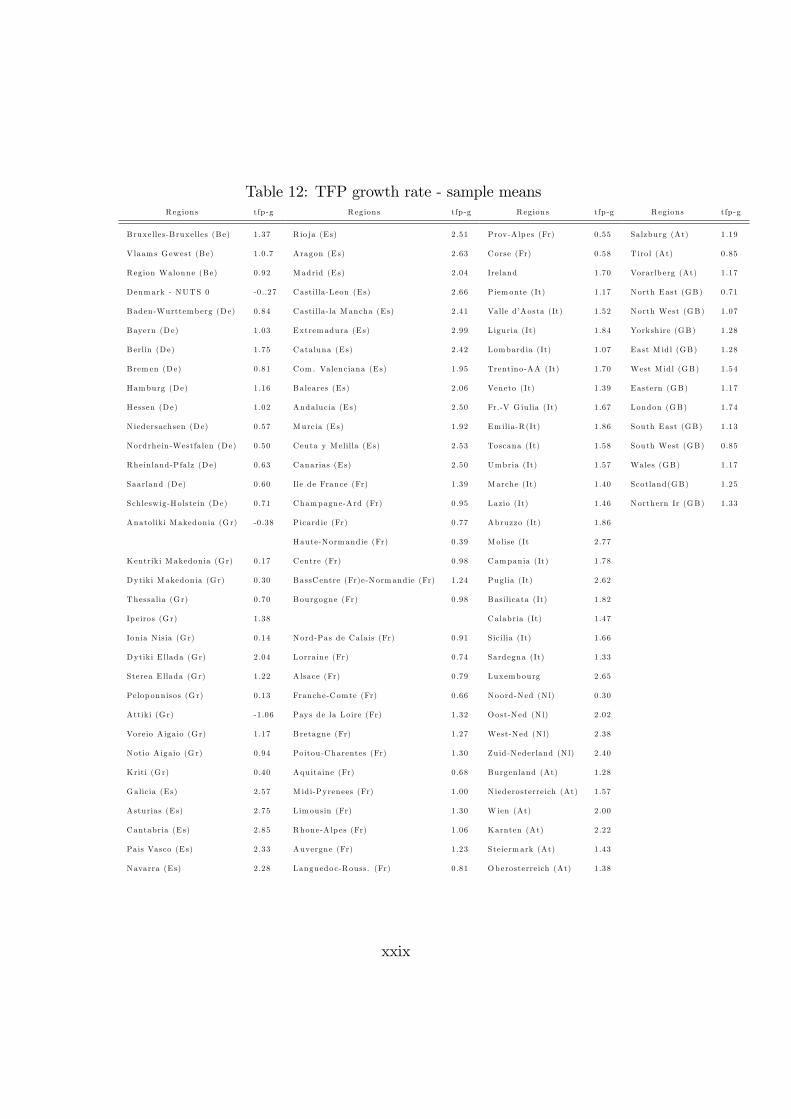
Table 12: TFP growth rate - sample meansRegions tfp -g


V laam s Gewest (Be) 1.0 .7


Denmark - NUTS 0 -0..27


Bayern (De) 1.03

Berlin (De) 1.75

Brem en (De) 0.81

Hamburg (De) 1.16

Hessen (De) 1.02




Saarland (De) 0.60


Anatolik i M akedonia (G r) -0 .38




Ip eiros (G r) 1.38





Attik i (G r) -1 .06



Kriti (G r) 0.40

Galic ia (Es) 2.57

Asturias (Es) 2.75

Cantabria (Es) 2.85


Navarra (Es) 2.28

Regions tfp -g

R io ja (Es) 2.51

Aragon (Es) 2.63

Madrid (Es) 2.04




Cataluna (Es) 2.42


Baleares (Es) 2.06

Andalucia (Es) 2.50

Murcia (Es) 1.92


Canarias (Es) 2.50





Centre (Fr) 0.98


Bourgogne (Fr) 0.98


Lorraine (Fr) 0.74

A lsace (Fr) 0.79



Bretagne (Fr) 1.27




L imousin (Fr) 1.30


Auvergne (Fr) 1.23


Regions tfp -g


Corse (Fr) 0.58

Ireland 1.70



L iguria (It) 1 .84



Veneto (It) 1 .39



Toscana (It) 1 .58

Umbria (It) 1 .57

Marche (It) 1 .40

Lazio (It) 1 .46

Abruzzo (It) 1 .86

Molise (It 2 .77

Campania (It) 1 .78

Puglia (It) 2 .62


Calabria (It) 1 .47

S icilia (It) 1 .66

Sardegna (It) 1 .33

Luxembourg 2.65







W ien (At) 2.00

Karnten (At) 2.22



Regions tfp -g

Salzburg (At) 1.19

T iro l (At) 0.85







Eastern (GB) 1.17

London (GB) 1.74



Wales (GB) 1.17

Scotland(GB) 1.25


xxix

0.5 Conclusion

This paper has analyzed the economic performance of a sample of European Re-

gions. It has provided estimates of Cobb-Douglas production functions over the

period 1976-2000. The sample was composed by 115 European Regions of 12

Countries: Austria, Belgium, Denmark, France, Germany, Greece, Ireland, Italy,

Luxembourg, Nethelands, Spain, United Kingdom. Great attention has been de-

voted to the estimation procedures. Because problems of non-stationarity may

arise when panel data approach is used to estimate the production function, the

�rst step of this work has been to investigate the properties of regional time se-

ries for value added, capital stock and labour. The presence of unit roots in the

series has been found and, consequently, I applied panel cointegration tests to

guard against the spurious regression problem. It has been clearly shown that

in the given panel all the variables share a long-run relationship and this implies

evidence in favour of a long-run production function relationship.

I have reported results for a �xed e¤ects GLS estimator to take account of

heteroskedasticity and serial correlation.

I have found a coe¢ cient for capital stock very close to the �ndings of the

accounting approach.

This paper also reports the estimated Total Factor Productivity for each region.

The results show remarkable di¤erences among regions in the technological knowl-

edge levels. In particular, some regions of France and Austria exhibit the highest

levels of TFP. On the other hand, the lowest parameters are those of regions of

Greece and Spain.

Looking at the results for Italian regions, the highest values are those of the

xxx

northern regions; the leader region is Valle d�Aosta, with a technological parameter

of (4:14). On the other hand, the lowest value are those for southern regions, with

Puglia exhibiting the lowest parameter (2:24). This �nding con�rms the well-

known dualism between North and South of Italy.

xxxi

Bibliography

[1] Arellano, M., and S.R. Bond (1991),"Some Tests of Speci�cation for Panel

Data: Monte Carlo Evidence and an Application to Employment Equations",

Review of Economic Studies, vol. 58, 277-97.

[2] Ark, B. van (1993), "Comparative Levels of Manufacturing Productivity in

Postwar Europe: Measurement and Comparison", Oxford Bulletin of Eco-

nomics and Statistics, vol. 52, 343-74.

[3] Baltagi, B. (1995), "Econometric Analysis of Panel Data", New York, NY,

Wiley.

[4] Barro, R.,and X. Sala-i-Martin (1995), "Economic Growth", New York,

McGraw-Hill.

[5] Barro, R., "Notes on Growth Accounting", mimeo, Harvard University, 1998

[6] Bernard, A.B. and C.I. Jones (1996), "Productivity Levels Across Countries",

Economic Journal, vol. 106, 1037-44.

[7] Breitung, J. and W. Meyer (1991), "Testing for Unit Root in Panel Data: Are

Wages on Di¤erent Bargaining Level Cointegrated?", Institut Fur Quantita-

tive Wirtschaftsforschung, Working Paper.

xxxii

[8] Canning, D. and P. Pedroni (1999), "Infrastructure and Long-run Economic

Growth", mimeo, Indiana University.

[9] Coakley, J. and A.M. Fuertes (1997), New Panel unit root tests of PPP,

Economic Letters, vol. 57, 17-22.

[10] Costello, D.M. (1993), "A Cross-Country, Cross-Industry Comparison of Pro-

ductivity Growth", Journal of Political Economy vol. 101, 207-22

[11] Dale, J.W. and Z. Griliches (1967), "The Explanation of Productivity

Change", Review of Economic Studies, vol. 34, 249-80.

[12] Dickey, D.A., and W.A. Fuller (1979), "Distribution of the Estimators for

Autoregressive Time Series with a Unit Root", Journal of the American Sta-

tistical

[13] Dollar D. and E.N. Wol¤ (1993), "Competitiveness, Convergence and Inter-

national Specialization", MIT Press, Cambrige, MA.

[14] Easterly, W., and R. Levine (2001), "It�s Not Factor Accumulation: Stylized

Facts and Growth Model", The World Bank Economic Review, vol. 15, 177-

219

[15] Hall R. and C. Jones (1996), "The Productivity of Nations", Department of

Economic, Stanford Univestity.

[16] Hall R. and C. Jones (1997), "Levels of Economic Activities Across Coun-

tries", American Economic Review, vol. 87, 173-177.

xxxiii

[17] Harrigan, J. (1995), "Factor Endowments and International Location of Pro-

duction: Econometric Evidence for the OECD, 1970-1985", Journal of Inter-

national Economics, vol. 39, 123-41.

[18] Harrigan, J. (1997a), "Technology, Factor Supplies and International Spe-

cialization: Estimating the Neoclassical Model", The American Economic

Review, vol. 87, 475-94.

[19] Harrigan, J. (1999), "Estimation of Cross-Country Di¤erences in Industry

Production", Journal of International Economics, vol. 114, 83-116

[20] Harris, R. (1995), "Cointegration Analysis in Econometric Modelling", Pren-

tice Hall.

[21] Hsaio, C. (1986), "Analysis of Panel Data", Cambridge University Press

[22] Hoon, H.T. and E. Phelps (1997), �Growth, Wealth and the Natural Rate: Is

Europe�s Job Crisis a Growth Crisis?,�European Economic Review vol. 41,

549-57.

[23] Im, K.S., M.H. Pesaran, and Y. Shin (2003), "Testing for Unit Root in Het-

erogeneous Panels", Journal of Econometrics, vol. 115, 53-74

[24] Islam, N. (1995), "Growth Empirics: A Panel Data Aproach", Quarterly Jour-

nal of Economics, vol. 110, 1127-170.

[25] Islam, N. (1999), "International Comparison of Total Factor Productivity: A

Review", Review of Income and Wealth, vol. 45, 493-518.

[26] Larsson, R., J. Lyhagen and M. Löthgren (2001), "Likelihood-based Cointe-

gration Tests in Heterogenous Panels", Econometrics Journal, vol. 4.

xxxiv

[27] Layard, R., S. Nickell and R. Jackman (1991), Unemployment. Macroeconomic

Performance and the Labour Market, Oxford University Press.

[28] Levin, A, C.F. Lin and C.S.J. Chu (1993), "Unit Root Tests in Panel Data:

Asymptotic and Finite Sample Properties", Universtiy of California, San

Diego, Discussion Paper.

[29] Levin, A, C.F. Lin and C.S.J. Chu (2002), "Unit Root Tests in Panel Data:

Asymptotic and Finite Sample Properties", Journal of Econometrics, vol.

108, 1-24.

[30] Lucas, R.E. (1988), "On The Mechanics of Economic Development", Journal

of Monetary Economics, vol. 22, 3-42.

Maddala, G.S. and S. Wu (1999), "A comparative Study of Unit Root Tests

with Panel Data and a New Simple Test", Oxford Bulletin of Economics and

Statistics, vol. 61, 631-52.

[31] Mankiw, N.G., D. Romer and D.Weil (1992), "A Contribution to the Empirics

of Economic Growth", Quarterly Journal of Economics, vol. 107, 407-37.

[32] Mankiw, N.G.(1995), "The Growth of Nations", Brooking Papers on Eco-

nomic Activity, Washington DC: Brooking Institution, vol. 1, 275-310.

[33] Marrocu, E., R. Paci and R. Pala (2000), "Estimation of Total Factor Pro-

ductivity for Regions and Sectors in Italy. A Panel Cointegration Approach",

Working Paper, Contributi di Ricerca Crenos.

xxxv

[34] Mauro, L. and G. Carmeci (2000), �Long Run Growth and Investment

in Education: Does Youth Unemployment Matter?,� University of Trieste

Di.S.E.S.Working Papers n. 69.

[35] Miller, S. and M. Upadhyay (2000), "The E¤ect of Openness, Trade Orienta-

tion and Human Capital on Total Factor Productivity", Journal of Develop-

ment Economics, vol. 63, 399-423.

[36] Nyblom, J. and A. Harvey (2000), "Test of Common Stochastic Trends",

Econometric Theory, vol. 16, 176-99.

[37] OECD (1990), Economic Outlook, OECD: Paris




Pedroni, P. (1995), "Panel Cointegration, Asymptotic and Finite Sample

Properties of Pooled Time Series Tests, with Application to the PPP Hy-

pothesis", Indiana University Working Paper in Economics, n. 95-013.

[41] Pedroni, P. (1999), "Critical Values for Cointegration Tests in Heterogeneous

Panels with Multiple Regressor", Oxford Bulletin of Economics and Statistics,

vol. 61, 653-79.

[42] Phillips, P.C.B. and H.R. Moon (1999), "Linear Regression Limit Theory for

Nonstationary Panel Data", Econometrica, vol. 67, 1057-111.

xxxvi

[43] Quah, D. (1994), "Exploiting Cross-Section Variations for Unit Root Inference

in Dynamic Data", Economics Letters, vol. 44, 9-19

[44] Romer, P. (1986), "Increasing Returns and Long-run Growth", Journal of

Political Economy, vol. 94, 1002-36.

[45] Romer, P. (1990), "Endogenous Technological Change", Journal of Political

Economy, vol. 98, 71-102

[46] Solow, R.M. (1956),�A Contribution to the Theory of Economic Growth�,

Quarterly Journal of Economics vol. 70, 65-95.

[47] Solow, R. (1957), "Technical Change and Aggregate Production Function",

Review of Economics and Statistics, vol. 39, 312-20.

[48] Tre�er, D. (1993), "International Factor Price Di¤erences: Leontief Was

Right!", Journal of Political Economy, vol. 101, 961-87.

[49] Tre�er, D. (1995), "The Case of The Missing Trade and Other Mysteries",

Americam Economic Review, vol. 85, 1029-46.

xxxvii

total factor productivity estimates for a sample of...

Documents