topological and simplicial models of identity types
TRANSCRIPT

arX
iv:1
007.
4638
v2 [
mat
h.L
O]
14
Oct
201
1
TOPOLOGICAL AND SIMPLICIAL
MODELS OF IDENTITY TYPES
BENNO VAN DEN BERG AND RICHARD GARNER
Abstract. In this paper we construct new categorical models for the identity typesof Martin-Lof type theory, in the categories Top of topological spaces and SSet ofsimplicial sets. We do so building on earlier work of Awodey and Warren, which hassuggested that a suitable environment for the interpretation of identity types should bea category equipped with a weak factorisation system in the sense of Bousfield–Quillen.It turns out that this is not quite enough for a sound model, due to some subtlecoherence issues concerned with stability under substitution; and so our first task isto introduce a slightly richer structure—which we call a homotopy-theoretic model ofidentity types—and to prove that this is sufficient for a sound interpretation.
Now, although both Top and SSet are categories endowed with a weak factorisa-tion system—and indeed, an entire Quillen model structure—exhibiting the additionalstructure required for a homotopy-theoretic model is quite hard to do. However, the cat-egories we are interested in share a number of common features, and abstracting theseleads us to introduce the notion of a path object category. This is a relatively simpleaxiomatic framework, which is nonetheless sufficiently strong to allow the constructionof homotopy-theoretic models. Now by exhibiting suitable path object structures onTop and SSet, we endow those categories with the structure of a homotopy-theoreticmodel: and, in this way, obtain the desired topological and simplicial models of identitytypes.
1. Introduction
Recently, there have been a number of interesting developments in the categoricalsemantics of intensional Martin-Lof type theory, with work such as [1, 4, 5, 6, 13, 20] es-tablishing links between type theory, abstract homotopy theory and higher-dimensionalcategory theory. All of this work can be seen as an elaboration of the following basic idea:that in Martin-Lof type theory, a type A is analogous to a topological space; elementsa, b ∈ A to points of that space; and elements of an identity type p, q ∈ IdA(a, b) to pathsor homotopies p, q : a → b in A. This article is a further development of this theme;its goal is to construct models of the identity types in categories whose objects have asuitably topological nature to them—in particular, in the categories of topological spacesand of simplicial sets.
One popular approach to articulating the topological nature of a category is to equipit with a model structure in the sense of [17]. It is shown in [1] that such a modelstructure is a suitable environment for the interpretation of the identity types of Martin-Lof type theory; the main point being that we may fruitfully interpret dependent types(x ∈ Γ)A(x) by fibrations A → Γ in the model structure. In fact, a model structure issomewhat more than one needs: it is comprised of two weak factorisation systems [2]
The second author acknowledges the support of the Centre for Australian Category Theory.
1

2 BENNO VAN DEN BERG AND RICHARD GARNER
interacting in a well-behaved manner, but as Awodey and Warren point out, in modellingtype theory only one of these weak factorisation systems plays a role.
Now, it is certainly the case that the categories of topological spaces and of simplicialsets carry well-understood Quillen model structures; and so one might expect that wecould construct models of identity types in them by a direct appeal to Awodey andWarren’s results. In fact, this is not the case due to a crucial detail—which we have sofar elided—concerning the stability under substitution of the identity type structure. Inthe categorical interpretation described by Awodey and Warren, substitution is modelledby pullback, whilst the identity type structure is obtained by choosing certain pieces ofdata whose existence is assured by the given weak factorisation system (henceforth w.f.s.).Thus to ask for the identity type structure to be stable under substitution is to ask forthese choices of data to be suitably stable under pullback, something which in general israther hard to arrange.
A finer analysis of this stability problem is given in [20], which reveals two distinctaspects to it. The first concerns the stability under substitution of the identity type itselfand of its introduction rule. For many examples derived from w.f.s.’s, including thosestudied in [20] and those studied here, it is possible—though by no means trivial—toobtain this stability by choosing one’s data with sufficient care. However, the secondaspect to the stability problem is more troublesome. It concerns the stability of theidentity type’s elimination and computation rules: and here we know rather few examplesof w.f.s.’s for which the requisite data may be chosen in a suitably coherent manner.
The first main contribution of this paper is to describe a general solution to thestability problem for homotopy-theoretic semantics. The key idea is to work with amild “algebraisation” of the notion of w.f.s.—which we term a cloven w.f.s.—in whichcertain of the data whose existence is merely assured by the definition of w.f.s. are nowprovided as part of the structure. In this setting, we may model dependent types notby fibrations, but rather by cloven fibrations: the difference being that whereas being afibration is a property of a map, being a cloven fibration is structure on it. This extrastructure will turn out to be just what we need to determine canonical, pullback-stablechoices of interpretation for the identity type elimination rule. We crystallise this idea byintroducing a notion of homotopy-theoretic model of type theory—this being a categoryequipped with a cloven w.f.s. and suitable extra data related to that w.f.s.—and provingour first main result, that every homotopy-theoretic model admits a sound interpretationof the identity types of Martin-Lof type theory.
Now, any reasonable w.f.s. on a category may be equipped with the structure ofa cloven w.f.s.: but it is by no means always the case that this cloven w.f.s. can bemade part of a homotopy-theoretic model of identity types. This is because the “extradata” required to do so—namely, a pullback-stable choice of factorisations for diago-nal morphisms X → X ×Y X—is not something we expect to exist in general. Thesecond main contribution of this paper is to describe a simple and widely applicableaxiomatic framework—that of a path object category—within which one may constructcloven w.f.s.’s which do carry this extra data. The fundamental axiom of our frameworkis one asserting the existence for every object X of the given category of a “path object”MX providing an internal category structure MX ⇒ X on X. From this we obtain acloven w.f.s. whose fibrations are the maps with the path-lifting property with respect tothis notion of path. The reason that this cloven w.f.s. may be equipped with the extradata required for a homotopy-theoretic model is that the notion of path object category

TOPOLOGICAL AND SIMPLICIAL MODELS OF IDENTITY TYPES 3
is “stable under slicing”: which is to say that any slice of a path object category is apath object category, and that any pullback functor between slices preserves the struc-ture. We may thereby construct pullback-stable factorisations of diagonals by factorisingX → X×Y X using the path object structure on the slice over Y . We encapsulate this inthe second main result of the paper, which shows that every path object category givesrise to a homotopy-theoretic model of type theory.
The third main contribution of our paper is to exhibit a number of instances of thenotion of path object category, hence obtaining a range of different models of identitytypes. Some of the models we obtain are already known, such as the groupoid modelof [8], and the chain complex model of [20]. More generally, our framework allows us tocapture a class of models described in [20] whose structure is determined by an intervalobject in a category. However, beyond these classes of known models, we obtain twoimportant new ones: the first in the category of topological spaces, and the second in thecategory of simplicial sets. Let us also note that Jaap van Oosten has communicated theexistence of a further instance of our axiomatic framework in the effective topos of [9];this extends his work in [15].
It is as well to point out also what we do not achieve in this article. The categoricalmodels that one builds from the syntax of Martin-Lof type theory turn out to be neitherhomotopy-theoretic models nor path object categories; and so there can be no hopeof a completeness result for intensional type theory with respect to semantics valued ineither kind of model. The reason for this is a certain strictness present in these structures,necessary for the arguments we make, but not present in the syntax. This same strictnessalso has ramifications for the simplicial and topological models we construct. In bothcases, the obvious choices of path object—given in the topological case by the assignation
X 7→ X [0,1] and in the simplicial case by X 7→ X∆1, where ∆1 denotes the simplicial
interval—are insufficiently strict to yield a path object structure, necessitating a subtlermodel construction using the notion of (topological or simplicial) Moore path. It remainsan open problem as to whether there is a more refined notion of homotopy-theoretic modelwhich admits both the syntax and the “naive” simplicial and topological interpretationsas examples.
The plan of the paper is as follows. We begin in Section 2 by recalling the syntax andsemantics of the type theory we will be concerned with. Then in Section 3, we introducethe notion of a homotopy-theoretic model of identity types, and prove that every suchmodel admits a sound interpretation of our type theory. Next, in Section 4, we introducethe axiomatic structure of a path object category; in Section 5, we give a number ofexamples of path object categories, including the category of topological spaces, and thecategory of simplicial sets; and in Section 6, we show that every path object categorymay be made into a homotopy-theoretic model of identity types, and so admits a soundinterpretation of our type theory. Finally, Section 7 fills in the combinatorial details ofthe construction of the path object category of simplicial sets.
2. Syntax and semantics of dependent type theory
In this Section, we gather together the required type-theoretic background: firstlydescribing the syntax of the type theory with which we shall work, and then the corre-sponding notion of categorical model.

4 BENNO VAN DEN BERG AND RICHARD GARNER
A type a, b : A
IdA(a, b) typeId-form;
A type a : A
r(a) : IdA(a, a)Id-intro;
(x, y : A, p : IdA(x, y), ∆(x, y, p)
)C(x, y, p) type
x : A, ∆(x, x, r(x)) ⊢ d(x) : C(x, x, r(x)) a, b : A p : IdA(a, b)
∆(a, b, p) ⊢ Jd(a, b, p) : C(a, b, p)Id-elim;
x, y : A, p : IdA(x, y), ∆(x, y, p) ⊢ C(x, y, p) typex : A, ∆(x, x, r(x)) ⊢ d(x) : C(x, x, r(x)) a : A
∆(a, a, r(a)) ⊢ Jd(a, a, r(a)) = d(a) : C(a, a, r(a))Id-comp.
Figure 1. Identity type rules
2.1. Intensional type theory. By intensional Martin-Lof type theory, we mean thelogical calculus set out in Part I of [14]. Our concern in the present paper will be withthe fragment of this theory containing only the basic structural rules together with therules for the identity types. We now summarise this calculus. It has four basic forms ofjudgement: A type (“A is a type”); a : A (“a is an element of the type A”); A = B type
(“A and B are definitionally equal types”); and a = b : A (“a and b are definitionallyequal elements of the type A”). These judgements may be made either absolutely, orrelative to a context Γ of assumptions, in which case we write them as
Γ ⊢ A type, Γ ⊢ a : A, Γ ⊢ A = B type and Γ ⊢ a = b : A
respectively. Here, a context is a list Γ = x1 : A1, x2 : A2, . . . , xn : An−1, whereineach Ai is a type relative to the context x1 : A1, . . . , xi−1 : Ai−1. There are now somerather natural requirements for well-formed judgements: in order to assert that a : A wemust first know that A type; to assert that A = B type we must first know that A type
and B type; and so on. We specify intensional Martin-Lof type theory as a collection ofinference rules over these forms of judgement. Firstly we have the equality rules, whichassert that the two judgement forms A = B type and a = b : A are congruences withrespect to all the other operations of the theory; then we have the structural rules, whichdeal with weakening, contraction, exchange and substitution; and finally, the logical rules,which specify the type-formers of our theory, together with their introduction, eliminationand computation rules. The only logical rules we consider in this paper are those forthe identity types, which we list in Figure 1. We commit the usual abuse of notationin leaving implicit an ambient context Γ common to the premisses and conclusions ofeach rule, and omitting the rules expressing stability under substitution in this ambientcontext. Let us remark also that in the rules Id -elim and Id -comp we allow the type Cover which elimination is occurring to depend upon an additional contextual parameter∆. We refer to these forms of the rules as the strong computation and elimination rules.Were we to add Π-types (dependent products) to our calculus, then these rules would beequivalent to the usual ones, without the extra parameter ∆; however, in the absence ofΠ-types, this extra parameter is essential to derive all but the most basic properties ofthe identity type.

TOPOLOGICAL AND SIMPLICIAL MODELS OF IDENTITY TYPES 5
2.2. Models of type theory. We now give a suitable notion of categorical model forthe dependent type theory we have just described. There are a number of essentiallyequivalent notions of categorical model we could use (see, for example, [3, 10, 16]); ofthese, we have chosen Pitts’ type categories since they minimise the amount of datarequired to construct a model, but still admit a precise soundness and completenessresult. We first recall from [16] the basic definition.
Definition 2.2.1. A type category is given by:
• A category C of contexts.• For each Γ ∈ C, a collection Ty(Γ) of types in context Γ.• For each A ∈ Ty(Γ), an extended context Γ.A ∈ C and a dependent projectionπA : Γ.A→ Γ.
• For each f : ∆ → Γ in C and A ∈ Ty(Γ), a type A[f ] ∈ Ty(∆) and a morphismf+ : ∆.A[f ] → Γ.A making the following square into a pullback:
(1)
∆.A[f ]f+
πA[f ]
Γ.A
πA
∆f
Γ .
A type category is said to be split if it satisfies the coherence axioms
(2) A[idΓ] = A, A[fg] = A[f ][g], (idΓ)+ = idA.Γ, (fg)+ = f+g+.
Remark 2.2.2. In [16], the coherence axioms of (2) are taken as part of the definitionof a type category. We do not do so here due to the nature of the type categories wewish to construct: in them, the types over Γ will be (structured) maps X → Γ and theoperation of type substitution will be given by pullback, an operation which is rarelyfunctorial on the nose. However, as is pointed out in [7], without the coherence lawsof (2), we cannot obtain a sound interpretation of the structural axioms of a dependenttype theory. The main result of that paper allows us to overcome this: when translatedinto our language, it says that any type category may be replaced by a split type categorywhich is equivalent to it in a suitable 2-category of type categories.
We now describe the additional structure required on a type category for it to modelidentity types. First we introduce some notation. Given A,B ∈ Ty(Γ), we write B+ asan abbreviation for B[πA] ∈ Ty(Γ.A). Thus we have a pullback square
Γ.A.B+(πA)
+
πB+
Γ.B
πB
Γ.A πAΓ
.
In particular, when A = B, the universal property of this pullback induces a diagonalmorphism δA : Γ.A→ Γ.A.A+ satisfying πA+ .δA = (πA)
+.δA = idΓ.A.
Definition 2.2.3. A type category has identity types if there are given:
• For each A ∈ Ty(Γ), a type IdA ∈ Ty(Γ.A.A+);• For each A ∈ Ty(Γ), a morphism rA : Γ.A→ Γ.A.A+. IdA with πIdA .ra = δA;

6 BENNO VAN DEN BERG AND RICHARD GARNER
• For each C ∈ Ty(Γ.A.A+. IdA) and commutative diagram
(3)
Γ.Ad
rA
Γ.A.A+. IdA .C
πC
Γ.A.A+. IdA idΓ.A.A+. IdA
a diagonal filler J(C, d) making both triangles commute.
We further require that this structure should be stable under substitution. Thus, for everymorphism f : ∆ → Γ in C, we require that IdA[f
++] = IdA[f ], and that the following twosquares should commute:
(4)
∆.A[f ]rA[f ]
f+
∆.A[f ].A[f ]+. IdA[f ]
f+++
Γ.A rAΓ.A.A+. IdA
(5)
∆.A[f ].A[f ]+. IdA[f ]
f+++
J(C[f ],d[f ])∆.A[f ].A[f ]+.IdA[f ] .C[f+++]
f++++
Γ.A.A+. IdAJ(C,d)
Γ.A.A+. IdA .C .
As discussed above, the most appropriate formulation of the identity type rules inthe absence of Π-types incorporates an extra contextual parameter in the eliminationand computation rules. However, the structure we have just described captures only theweaker forms in which this contextual parameter is absent. Let us therefore formulatethe strong computation and elimination rules in our categorical setting.
Definition 2.2.4. A type category has strong identity types if for every A ∈ Ty(Γ) thereare given IdA and rA as above, but now for every
B1 ∈ Ty(Γ.A.A+. IdA)
...
Bn ∈ Ty(Γ.A.A+. IdA .B1 . . . Bn−1)
C ∈ Ty(Γ.A.A+. IdA .B1 . . . Bn−1.Bn)
and commutative diagram
(6)
Γ.A.∆[rA]d
(rA)+···+
Γ.A.A+. IdA .∆.C
πC
Γ.A.A+. IdA .∆ idΓ.A.A+. IdA .Λ
(where we write ∆ as an abbreviation for B1 . . . Bn in the obvious way), we are given adiagonal filler J(Λ, C, d) making both triangles commute. We require all this structureto be stable under substitution as in Definition 2.2.3.

TOPOLOGICAL AND SIMPLICIAL MODELS OF IDENTITY TYPES 7
By a categorical model of identity types, we mean a type category with strong identitytypes.
Remark 2.2.5. As discussed in Remark 2.2.2 above, our use of non-split type categoriesis justified by the coherence result of [7], which allows us to replace any non-split typecategory by an equivalent split one. For this justification to remain meaningful in thepresence of identity types, it must be the case that a (strong) identity type structure on atype category induces a corresponding structure on its strictification. This is indeed thecase, as proven in [20, Theorem 2.48]. (Actually, Warren does not consider the strongidentity type rules; but his argument may be modified without difficulty to cover thiscase.)
3. Homotopy-theoretic models of identity types
In this section, we define a notion of homotopy-theoretic model of identity types—building on the work of [1]—and prove our first main result, Theorem 3.3.5, which showsthat any homotopy-theoretic model gives rise to a categorical one. The notion of modeldescribed here can be seen as a precise formulation of one that is implicit in Chapter 3of [20].
3.1. Interpretation of identity types in a weak factorisation system. The notionof homotopy-theoretic model which we are going to define is based on the central ideaof [1]: that a suitable environment for the interpretation of identity types is that of acategory equipped with a weak factorisation system in the sense of [2]. We begin byrecalling the basic definitions.
Definition 3.1.1. A weak factorisation system or w.f.s. (L,R) on a category E is givenby two classes L and R of morphisms in E which are each closed under retracts whenviewed as full subcategories of the arrow category E2, and which satisfy the followingtwo axioms:
(i) Factorisation: each f ∈ E may be written as f = pi where i ∈ L and p ∈ R.(ii) Weak orthogonality : for each f ∈ L and g ∈ R, we have f � g,
where to say that f � g holds is to say that for each commutative square
(7)
Uh
f
X
g
Vk
Y
we may find a filler j : V → X satisfying jf = h and gj = k.
Given a category E equipped with a w.f.s., [1] suggests the following method of inter-preting identity types in it. One begins by taking the dependent types over some Γ ∈ Eto be the collection of R-maps X → Γ, with type substitution being given by pullback.Now given a map x : X → Γ ∈ E interpreting some dependent type over Γ, we mayfactorise the diagonal X → X ×Γ X as
(8) Xix−→ I(x)
jx−−→ X ×Γ X ,
where ix is an L-map, and jx an R-map. Since jx is an R-map, it gives rise to adependent type over X ×Γ X, which will be the interpretation of the identity type on

8 BENNO VAN DEN BERG AND RICHARD GARNER
X. The introduction rule for IdX will be interpreted by the map ix; whilst to interpretthe elimination and computation rules, we observe that given a diagram like (3) in E ,the left-hand arrow is in L—since it is the map ix above—and the right-hand arrow isin R—by definition of dependent type in the model—so that by weak orthogonality, wehave a filler J(C, d) as required.
3.2. Cloven weak factorisation systems. As discussed in the Introduction, when wetry to make the above argument precise we run into a problem of coherent choice. Thedefinition of weak factorisation system demands the existence of certain pieces of data—factorisations and diagonal fillers—without asking for explicit choices of these data tobe made. In order to model type theory, therefore, we must first choose factorisationsas in (8), and fillers for squares such as (3). However, we cannot make such choicesarbitrarily, since the categorical structure defining the identity types is required to bestable under substitution, which amounts to requiring that the choices of factorisationsand fillers we make be stable under pullback. As noted in the Introduction, the twoaspects of this requirement—stability of factorisations, and stability of fillers—are quitedifferent in nature. For whilst many naturally-occurring weak factorisation systems maybe equipped with stable factorisations (8)—as is worked out comprehensively in [20]—rather few have been similarly provided with stable fillers (3). A closer analysis of theexamples where this has been possible shows that underlying each of them is a structurericher than that of a mere w.f.s. The following definition is intended to capture theessence of that extra structure.
Definition 3.2.1. A cloven w.f.s. on a category E is given by the following data:
• For each f : X → Y in E , a choice of factorisation
(9) f = Xλf−−→ Pf
ρf−−→ Y ;
• For each commutative square of the form (7), a choice of diagonal fillers
(10)
Uλg .h
λf
Pg
ρg
Pfk.ρf
P (h,k)
Y
making the assignation (h, k) 7→ P (h, k) functorial in (h, k) ;
• For each f : X → Y , choices of fillers σf and πf as indicated:
(11)
Xλλf
λf
Pλf
ρλf
Pf1Pf
σf
Pf
and
Pf1Pf
λρf
Pf
ρf
Pρf ρρf
πf
Y .
To justify the nomenclature, we must show that any cloven w.f.s. has an underlyingw.f.s. To do this, we introduce the notion of cloven L- and R-maps in a cloven w.f.s. Bya cloven L-map structure on a morphism f : X → Y of E , we mean a map s : Y → Pf

TOPOLOGICAL AND SIMPLICIAL MODELS OF IDENTITY TYPES 9
rendering commutative the diagram
Xλf
f
Pf
ρf
Y1Y
s
Y .
We will sometimes express this by saying that (f, s) : X → Y is a cloven L-map. Dually, acloven R-map structure on f is given by a morphism p : Pf → X rendering commutativethe diagram
X1X
λf
X
f
Pfρf
p
Y .
Again, we may express this by calling (f, p) : X → Y a cloven R-map.
Proposition 3.2.2. Given a cloven L-map (f, s) : U → V , a cloven R-map (g, p) : X →Y and a commutative square of the form (7), there is a canonical choice of diagonal fillerj : V → X making both induced triangles in (7) commute.
Proof. We take j to be the composite Vs−→ Pf
P (h,k)−−−−→ Pg
p−→ X. �
The following result is now essentially Section 2.4 of [18]:
Corollary 3.2.3. Every cloven w.f.s. has an underlying w.f.s. whose two classes of mapsare given by
L := { f : A→ B there is a cloven L-map structure on f }
R := { g : C → D there is a cloven R-map structure on g } .
Proof. Firstly, it’s easy to show that L and R are closed under retracts. Secondly, foreach f : X → Y we have λf ∈ L since (λf , σf ) is a cloven L-map, and ρf ∈ R since(ρf , πf ) is a cloven R-map; and so we have the factorisation axiom. Finally, we mustshow that f � g for all f ∈ L and g ∈ R. But to do this we pick a cloven L-map structureon f and a cloven R-map structure on g and then apply the preceding Proposition. �
3.3. Homotopy-theoretic models of identity types. Let us now see how the notionof cloven w.f.s. allows us to resolve the problem of coherent choice with regard to fillers forsquares like (3). The idea is to refine our previous interpretation by taking the dependenttypes over some Γ ∈ C to be cloven R-maps X → Γ. For each such map, we demand theexistence of a factorisation of the diagonal X → X ×Γ X into a cloven L-map followedby a cloven R-map; whereupon Proposition 3.2.2 provides us with canonical choices offillers for squares like (3). Now by asking that the choices of factorisation in (8) aresuitably stable under substitution—as we do in Definition 3.3.3 below—we may ensurethe stability of the corresponding fillers in (3) by exploiting a “naturality” property ofthe liftings provided by Proposition 3.2.2. In order to describe this property, we firstneed a definition.

10 BENNO VAN DEN BERG AND RICHARD GARNER
Definition 3.3.1. If (f, s) : U → V and (g, t) : X → Y are cloven L-maps, then by amorphism of cloven L-maps (f, s) → (g, t) we mean a commutative square (7) such thatP (h, k).s = t.k. We write L-Map for the category of cloven L-maps and cloven L-mapmorphisms. Dually, we have the notion of morphism of cloven R-maps, giving the arrowsof a category R-Map.
It is now easy to verify the following:
Proposition 3.3.2. The choices of filler given by Proposition 3.2.2 are natural, in thesense that precomposing a square like (7) with a morphism of cloven L-maps (f ′, s′) →(f, s) sends chosen fillers to chosen fillers, as does postcomposing it with a morphism ofcloven R-maps (g, p) → (g′, p′).
There is one final point which we have not yet addressed. In the preceding discussion,we have outlined how we might obtain an interpretation of identity types in a homotopy-theoretic setting. What we have not discussed is how to interpret the strong eliminationand computation rules. Now, to ask for an interpretation of the strong rules is to askfor coherent choices of diagonal filler for squares of the form (6). In such a square weknow that the arrow πC down the right-hand side is a cloven R-map, so that if we couldshow that the map (rA)
+···+ down the left-hand side was a cloven L-map, then we couldonce again obtain the desired liftings by applying Proposition 3.2.2. But observing that(rA)
+···+ is the pullback of rA along a composite of dependent projections, we obtain thedesired conclusion whenever our cloven w.f.s. satisfies—in a suitably functorial form—theFrobenius property, that the pullback of any cloven L-map along a cloven R-map shouldagain be a cloven L-map. Note that this property has been considered before in thecontext of Martin-Lof type theory: see [4, Proposition 14] and [6, Definition 3.2.1], forexample.
With this last detail in place, we are now ready to give our notion of homotopy-theoretic model.
Definition 3.3.3. Suppose that E is a finitely complete category equipped with a clovenw.f.s.
(i) A choice of diagonal factorisations is an assignation which to every cloven R-map(x, p) : X → Γ associates a factorisation
(12) Xix−→ I(x)
jx−−→ X ×Γ X
of the diagonal X → X ×Γ X, together with a cloven L-map structure on ix and acloven R-map structure on jx.
(ii) A choice of diagonal factorisations is functorial if the assignation of (12) providesthe action on objects of a functor R-Map → R-Map ×E L-Map. Explicitly, thismeans that for every morphism of R-maps (f, g) : (x, p) → (y, q), there is given anarrow I(f, g) : I(x) → I(y), functorially in (x, p), and in such a way that the squares
(13)
X
ix
fY
iy
I(x)I(f,g)
I(y)
and
I(x)
jx
I(f,g)I(y)
jy
X ×Γ Xf×gf
Y ×∆ Y
are morphisms of L-maps and of R-maps respectively.

TOPOLOGICAL AND SIMPLICIAL MODELS OF IDENTITY TYPES 11
(iii) A functorial choice of diagonal factorisations is stable when for every morphismof R-maps (f, g) : (x, p) → (y, q) whose underlying morphism in E2 is a pullbacksquare, the right-hand square in (13) is also a pullback.
(iv) The cloven w.f.s. is Frobenius if to every pullback square
f∗Xf
ı
X
i
Bf
A
with f a cloven R-map and i a cloven L-map, we may assign a cloven L-mapstructure on ı. It is functorially Frobenius if this assignation gives rise to a functorR-Map×E L-Map → L-Map.
A homotopy-theoretic model of identity types is a finitely complete category E equippedwith a cloven w.f.s. which is functorially Frobenius and has a stable functorial choice ofdiagonal factorisations.
Remark 3.3.4. Note that any cloven w.f.s. has an obvious functorial choice of diagonalfactorisations: given an R-map (x, p) : X → Γ, we factorise the diagonal morphismδx : X → X×ΓX as (λδx , ρδx), with the cloven L- and R- structures given by σδx and πδx .However, this choice is not a particularly useful one for our purposes, since it is almostnever stable. It will be the task of the next section, and the second main contribution ofthis paper, to describe a general structure—that of a path object category—from whichwe may construct cloven w.f.s.’s which do have a stable functorial choice of diagonalfactorisations.
The remainder of this section will be devoted to proving our first main result:
Theorem 3.3.5. A homotopy-theoretic model of identity types is a categorical model ofidentity types.
We begin by defining the type category associated to a cloven w.f.s.
Proposition 3.3.6. Let E be a finitely complete category equipped with a cloven w.f.s.Then there is a type category whose category of contexts is E, and whose collection oftypes over Γ ∈ E is the set of cloven R-maps with codomain Γ.
Proof. For A ∈ Ty(Γ) corresponding to a cloven R-map (x, p) : X → Γ, we define theextended context Γ.A to beX and the dependent projection πA : Γ.A→ Γ to be x. Givenfurther a morphism f : ∆ → Γ of E , we must define a type A[f ] ∈ Ty(∆) and a morphismf+ : ∆.A[f ] → Γ.A. So let the following be a pullback diagram in E :
Yg
y
X
x
∆f
Γ .

12 BENNO VAN DEN BERG AND RICHARD GARNER
Now let q : Py → Y be the morphism induced by the universal property of pullback inthe following diagram:
Pyp.P (g,f)
ρh
X
x
∆f
Γ .
It’s easy to check that this makes (y, q) : Y → ∆ into a cloven R-map, which we define tobe A[f ] ∈ Ty(∆). Now we take f+ : ∆.A[f ] → Γ.A to be g, which clearly makes (1) intoa pullback as required. Let us observe for future reference that the pair (g, f) determinesa morphism of R-maps (y, q) → (x, p); and that q is in fact the unique cloven R-mapstructure on y for which this the case. �
We now show that in the presence of a stable functorial choice of diagonal factorisations,the type category constructed by the preceding Proposition has identity types which arestable under substitution.
Proposition 3.3.7. Let E be a finitely complete category bearing a cloven w.f.s. that isequipped with a stable functorial choice of diagonal factorisations. Then the associatedtype category of Proposition 3.3.6 has identity types.
Proof. Suppose given A ∈ Ty(Γ). To define IdA, we observe that the square
Γ.A.A+(πA)
+
πA+
Γ.A
πA
Γ.A πAΓ
is a pullback; so by assumption, we have a factorisation of the diagonal morphismδA : Γ.A→ Γ.A.A+ as
Γ.AiπA−−−→ I(πA)
jπA−−−→ Γ.A.A+
where iπA is a cloven L-map and jπA a cloven R-map. We now take the identity typeIdA ∈ Ty(Γ.A.A+) to be the cloven R-map jπA , and take the introduction morphismrA : Γ.A → Γ.A.A+. IdA to be iπA . Note that πIdA .rA = jπA .iπA = δA as required. Asfor the elimination and computation rules, let us suppose given C ∈ Ty(Γ.A.A+. IdA)and a commutative square of the form (3). In such a square, the dependent projectionπC comes with an assigned cloven R-map structure, whilst rA bears a cloven L-mapstructure (since it is iπA); and so by Proposition 3.2.2, we obtain the required choice ofdiagonal filler J(C, d) : Γ.A.A+. IdA → Γ.A.A+. IdA .C.
It remains to verify the stability of the above structure under substitution. Firstly,given A ∈ Ty(Γ) and f : ∆ → Γ in E , we must show that IdA[f
++] = IdA[f ]. But itfollows from stability of the choice of diagonal factorisations that there is a pullback

TOPOLOGICAL AND SIMPLICIAL MODELS OF IDENTITY TYPES 13
square
∆.A[f ].A[f ]+. IdA[f ]θ
πIdA[f ]
Γ.A.A+. IdA
πIdA
∆.A[f ].A[f ]+f++ Γ.A.A+
in E ; and so it suffices to show that in this square, pulling back the assigned cloven R-mapstructure on the right-hand arrow yields the assigned R-map structure on the left-handone. For this we observe that—by functoriality of the choice of diagonal factorisations—when both vertical maps are equipped with their assigned R-map structures, the dis-played square comprises a morphism of R-maps. But by the remark concluding theproof of Proposition 3.3.6, this condition characterises uniquely the R-map structure in-duced by pullback on the left-hand arrow; so that the pullback R-map structure coincideswith the assigned one, as required.
Finally, we verify commutativity of the diagrams (4) and (5). For the former, thisfollows immediately from functoriality of the choice of diagonal factorisations; whilst forthe latter, we observe that—again by functoriality—the vertical maps in (4) comprise amorphism of cloven L-maps from rA[f ] to rA; and that in the pullback diagram
∆.A[f ].A[f ]+. IdA[f ] .C[f+++]f++++
πC[f+++]
Γ.A.A+. IdA .C
πC
∆.A[f ].A[f ]+. IdA[f ]f+++
Γ.A.A+. IdA ,
the horizontal arrows comprise a morphism of cloven R-maps from πC[f+++] to πC . Com-mutativity in (5) therefore follows from Proposition 3.3.2. �
This does not quite complete the proof of Theorem 3.3.5, since a categorical modelof identity types must model the strong elimination and computation rules, whereas theprevious Proposition only indicates how to model the standard ones. For this we makeuse the Frobenius property of a homotopy-theoretic model:
of Theorem 3.3.5. By Proposition 3.3.7, we know that we already have a type categorywith identity types; hence it suffices to show that these identity types are strong. Sosuppose given a commutative diagram as in (6). By assumption, πC is a cloven R-map;and by repeated application of the Frobenius structure, (rA)
+···+ is a cloven L-map;and so we may once again apply Proposition 3.2.2 to obtain the required diagonal filler.All that remains is to verify the stability of these new fillers under substitution; andthis follows exactly as before, but now using also the functoriality of the Frobeniusstructure. �
4. Path object categories
We have now described the notion of a homotopy-theoretic model of identity types,and shown that any such gives rise to a categorical model. However, as we noted in Re-mark 3.3.4, it is in practice rather hard to verify that a category satisfies the axioms fora homotopy-theoretic model. We are therefore going to introduce a further set of axioms

14 BENNO VAN DEN BERG AND RICHARD GARNER
which are much simpler to verify, but still sufficiently strong to allow the constructionof a homotopy-theoretic model. We call a category satisfying these axioms a path objectcategory. This section gives the definition; the following one provides a number of exam-ples; and Section 6 proves our second main result, that every path object category givesrise to a homotopy-theoretic model of identity types.
4.1. Path objects. Throughout the rest of this section, we assume given a finitelycomplete category E . The first piece of structure that we will require is a choice of “pathobject” for each object of E .
Axiom 1. For every X ∈ E , there is given an internal category
X rX MX
sX
tX
MX sX×tX MXmX
.
together with an involution τX : MX → MX which defines an internal identity-on-objects isomorphism between the category MX and its opposite. We require this struc-ture to be functorial in X—thus the assignation X 7→ MX should underlie a functorE → E , and the maps sX , tX , mX , rX and τX should be natural in X—and that thefunctor M should preserve pullbacks.
Remark 4.1.1. We may rephrase the above in a number of ways. The naturality of r,m, s and t is equivalent to asking that every morphism f : X → Y of E should inducean internal functor (f,Mf) : (X,MX) → (Y,MY ); and this is in turn equivalent toasking that we should have a functor E → Cat(E) which is a section of the functorob: Cat(E) → E .
The example that we have in mind—which will be developed in more detail in thefollowing section—is the category of topological spaces. Here the first thing one mighttry is to take MX := X [0,1], with rX and mX given by the constant path and con-catenation of paths respectively. However, this definition fails to satisfy the categoryaxioms, since concatenation of paths is only associative and unital “up to homotopy”.To rectify this, we take MX instead to be the Moore path space of X, given by the set{ (r, φ) r ∈ R+, φ : [0, r] → X } equipped with a suitable topology (detailed in Section 5below). Now rX sends a point of X to the path of length 0 at that point, whilst mX
takes paths of length r and s respectively to the concatenated path of length r+s. Withthis definition, we determine an internal category MX ⇒ X as required.
4.2. Strength. Returning to our axiomatic framework, the next piece of structure wewish to encode is a way of contracting a path onto one of its endpoints. As a first attemptat formalising this, we might require that for every path φ : a→ b in X there be given a“path of paths” ηX(φ) of the form indicated by the following diagram:
aφ
φηX(φ)
b
rX(b)
brX(b)
b
.

TOPOLOGICAL AND SIMPLICIAL MODELS OF IDENTITY TYPES 15
This amounts to asking for a morphism ηX : MX → MMX which yields the identityupon postcomposition with sMX orMsX , and yields the composite rX .tX upon postcom-position with tMX or MtX . However, this formalisation fails to capture our motivatingtopological example. Indeed, for a Moore path φ : a → b ∈ MX of length r, the cor-responding path of paths ηX(φ) must also be of length r, since MsX preserves pathlength and we require that MsX(ηX(φ)) = φ. But then whenever r > 0 we cannot haveMtX(ηX(φ)) = rX(b), since MtX also preserves path length and rX(b) is of length 0.
We must therefore refine our formalisation. In the motivating topological case, we cando this by requiring that MtX(ηX(φ)) be not a path of length 0, but rather a path ofthe same length as φ, but constant at b. In order to capture the idea of a non-identity,but constant, path in our abstract framework, we introduce a further piece of structure.
Axiom 2. The endofunctor M comes equipped with a strength [12]
αX,Y : MX × Y →M(X × Y )
with respect to which s, t, r, m and τ are strong natural transformations.
In fact, such a strength is determined, up to natural isomorphism, by its componentsof the form α1,X : M1×X →MX, since every square of the following form is a pullback:
(14)
MX × YαX,Y
M !×Y
M(X × Y )
Mπ2
M1× Y α1,YMY .
To see this, we consider the diagram
MX × YαX,Y
M !×Y
M(X × Y )Mπ1
Mπ2
MX
M !
M1× Y α1,YMY
M !M1 .
In it, the right-hand square is a pullback since M preserves pullbacks, and the outersquare is a pullback since the composites along the top and bottom are equal, by natu-rality of α, to π1. Hence the left-hand square is also a pullback as claimed.
We may give the following interpretation of the components α1,X . The object M1 wethink of as the “object of path lengths”, and the morphism α1,X : M1 × X → MX astaking a length r ∈M1 and an element x ∈ X and returning the path of length r whichis constant at x. In fact, by naturality of α in Y together with strength of t, we see thatthe diagram
(15) M1×Xα1,X−−−→MX
(M !, tX )−−−−−→M1×X
exhibits M1 × X as a retract of MX, so that we may think of M1 × X as being the“subobject of constant paths” of MX. In our topological example, we have a strengthαX,Y that takes a Moore path (r, φ) ∈ MX and a point y ∈ Y and returns the path(r, ψ) ∈ M(X × Y ), where ψ(s) = (φ(s), y). Now the subspace of MX determined bythe retract (15) is comprised precisely of the constant paths of arbitrary length in X, asdesired.

16 BENNO VAN DEN BERG AND RICHARD GARNER
4.3. Path contraction. With the aid of Axiom 2, we may now formalise the structureallowing the contraction of a path onto its endpoint. Observe that it is in equation (19)that we make use of the notion of constant path.
Axiom 3. There is given a strong natural transformation η : M ⇒MM such that thefollowing equations hold:
sMX .ηX = idMX(16)
tMX .ηX = rX .tX(17)
MsX .ηX = idMX(18)
MtX .ηX = α1,X .(M !, tX)(19)
ηX .rX = rMX .rX .(20)
Definition 4.3.1. By a path object category, we mean a finitely complete category Esatisfying Axioms 1, 2 and 3.
Our motivation for introducing the notion of path object category is the followingtheorem, whose proof we give in Section 6 below.
Theorem 4.3.2. A path object category is a homotopy-theoretic model of identity types;and hence also a categorical model of identity types.
Remark 4.3.3. The above structure is in fact slightly more than is necessary for ourargument. Axiom 1 posits an internal category structure MX ⇒ X on each object Xof E , but we will make no use at all of the associativity of composition in these internalcategories, and need right unitality only at one particular (though crucial) point; on theother hand, we will make repeated and unavoidable use of left unitality. Now, for theexamples we have in mind, it happens that, in ensuring the unitality axioms, we alsoobtain associativity: but in recognition of other potential examples where this may notbe so, we give a more precise delineation of what is needed. On replacing Axiom 1 by thefollowing weaker Axiom 1′, we may still carry through the entire proof of Theorem 4.3.2,as given in Section 6 below; and on replacing it by the yet weaker Axiom 1′′, may still carryout at least the arguments of Sections 6.1 and 6.3, though that of Section 6.2 does notgo through, as without right unitality we cannot complete the proof of Proposition 6.2.2.
Axiom 1′. As Axiom 1, but drop associativity of composition, and functoriality of τwith respect to binary composition. Explicitly, this means that for every X ∈ E , thereis given, functorially in X, a diagram
X rX MX
τXsX
tX
MX sX×tX MXmX ,
such that M preserves pullbacks, and such that the following equations hold:
sX .rX = 1X mX(rX .tX , 1MX) = 1MX
tX .rX = 1X sX .τX = tX
sX .mX = sX .π2 tX .τX = sX
tX .mX = tX .π1 rX = τX .rX
mX(1MX , rX .sX) = 1MX τX .τX = 1X .

TOPOLOGICAL AND SIMPLICIAL MODELS OF IDENTITY TYPES 17
Axiom 1′′. As Axiom 1′, but drop also the right unitality axiom (uppermost in theright-hand column of the preceding list).
In spite of the above, we shall continue to write as if the stronger Axiom 1 were satisfied,for two reasons. Firstly, this allows us all the terminological conveniences afforded bythe language of internal category theory; and secondly, as noted above, in each of theexamples we shall now give it is the stronger Axiom 1 that holds.
5. Examples of path object categories
5.1. Topological spaces.
Proposition 5.1.1. The category of topological spaces may be equipped with the structureof a path object category.
Proof. As discussed above, we cannot define the path space MX of a topological spaceX to be X [0,1], since composition of paths [0, 1] → X is associative and unital only “upto homotopy”. Instead, we consider paths of varying lengths and the Moore path space
MX = {(ℓ, φ) | ℓ ∈ R+, φ : [0, ℓ] → X} .
(Here R+ denotes the set of non-negative real numbers.) To define a suitable topologyon MX, we observe that there is a monomorphism MX → R+ ×XR+ sending (ℓ, φ) tothe pair (ℓ, φ), where φ is defined by
φ(x) =
{φ(x) if x ≤ ℓ,φ(ℓ) if x ≥ ℓ.
We may therefore topologiseMX as a subspace of R+×XR+ , where the latter is equipped
with its natural topology (coming from the product and the compact-open topology). Wehave continuous projections sX , tX : MX ⇒ X sending (ℓ, φ) to φ(0) and φ(ℓ) respec-tively; and as is well-known, the topological graph this defines bears the structure of atopological category, with the identity rX(x) being the constant path at x of length 0,and the composition mX of paths (ℓ, φ) and (m,ψ) being the path χ of length ℓ + mgiven by:
χ(x) =
{φ(x) if x ≤ ℓ,ψ(x− ℓ) if x ≥ ℓ.
Moreover, this topological category bears an involution τX , which sends a path φ of lengthℓ to the same path in reverse: that is, the path φo of length ℓ with φo(x) = φ(ℓ− x).
We now define a strength αX,Y : MX ×Y →M(X ×Y ) by sending the pair ((ℓ, φ), y)to the path ψ of length ℓ in X × Y defined by ψ(x) = (φ(x), y). Finally, the mapsηX : MX →MMX are given by contracting a path to its endpoint: so we take ηX(ℓ, φ)to be the path ψ in MX of length ℓ whose value at x ≤ ℓ is the path of length ℓ − xgiven by ψ(x)(y) = φ(x + y). We have now given all the data required for a pathobject category; the remaining verifications are entirely straightforward and left to thereader. �
Corollary 5.1.2. The category of topological spaces may be equipped with the structureof a categorical model of identity types. In this model, propositional equalities betweenterms of closed type are interpreted by Moore homotopies.

18 BENNO VAN DEN BERG AND RICHARD GARNER
5.2. Groupoids. In our next few examples, we revisit some previously constructed mod-els of identity types and show that they fit into our framework, beginning with one ofthe earliest instances of a higher-dimensional model of type theory: the groupoid modelof [8].
Proposition 5.2.1. The category of small groupoids bears a structure of path objectcategory.
Proof. Let I be the groupoid with two objects 0 and 1 and two non-identity arrows 0 → 1and 1 → 0 (which clearly must be each others’ inverses). Now for any groupoid X, wedefine MX = XI ; so the objects of MX are the arrows in X and the morphisms ofMX are commutative squares. The functors sX , tX : MX → X are obtained by takingdomains and codomains, respectively, whilst the functor rX : X →MX sends an objectof X to the identity arrow at that object. The functor mX : MX ×XMX →MX sendsa pair of arrows (g, f) to their composite gf ; whilst τX : MX → MX sends each arrowto its inverse. It is immediate that these data equip X with the structure of an internalgroupoid. We obtain the strength αX,Y : MX × Y → M(X × Y ) by mapping an arrowf of X and an object y of Y to the arrow (f, idy) of X × Y ; and finally, we define themaps ηX : MX →MMX by sending an arrow f : a→ b of X to the commuting square
af
f
b
id
bid
b .
Again, the remaining verifications are straightforward. �
Corollary 5.2.2. The category of small groupoids may be equipped with the structureof a categorical model of identity types. In this model, propositional equalities betweenterms of closed type are interpreted by natural isomorphisms between functors.
5.3. Chain complexes. For our next example we consider chain complexes over a ring.The model of type theory this induces is also constructed in [20].
Definition 5.3.1. Let R be a ring. A chain complex over R is given by a collectionA = (An |n ∈ Z) of left R-modules, together with maps ∂n : An → An−1 satisfying∂n∂n+1 = 0 for all n ∈ Z. Given chain complexes A and B, a chain map A → B is afamily of maps (fn : An → Bn |n ∈ Z) such that ∂n ◦ fn = fn−1 ◦ ∂n for all n ∈ Z.
Proposition 5.3.2. The category of chain complexes over a ring R bears the structureof a path object category.
Proof. For a chain complex A, we define the path object MA by
(MA)n = An ⊕An+1 ⊕An,
∂n(a, f, b) = (∂na, b− a− ∂n+1f, ∂nb).
The source and target maps sA, tA : MA → A are given by first and third projectionrespectively, whilst rA : A → MA is given by rA(a) = (a, 0, a). In order to definethe composition map mA : MA ×A MA → MA, note that we have (MA ×A MA)n ∼=An ⊕ An+1 ⊕ An ⊕ An+1 ⊕ An, so that we may take mA(a, f, b, g, c) = (a, f + g, c).Finally, the involution τA : MA → MA is given by τA(a, f, b) = (b,−f, a). It is easy

TOPOLOGICAL AND SIMPLICIAL MODELS OF IDENTITY TYPES 19
to see that all the maps defined so far are chain maps and give A the structure of aninternal groupoid. Note that M preserves pullbacks, as it does so degreewise; in fact,it also preserves the terminal object 0, and hence all finite limits. We give a strengthαA,X : MA ⊕X → M(A ⊕X) by αA,X
((a, f, a′), x
)=
((a, x), (f, 0), (a′, x)
). Finally, to
give the maps ηA : MA→MMA, we observe that since
(MMA)n = (An ⊕An+1 ⊕An)⊕ (An+1 ⊕An+2 ⊕An+1)⊕ (An ⊕An+1 ⊕An) ,
we may take ηA(a, f, b) =((a, f, b), (f, 0, 0), (b, 0, b)
). The remaining verifications are
entirely straightforward. �
Recall that if f, g : A → B are chain maps, then a chain homotopy γ : f ⇒ g is acollection of R-module maps γn : An → Bn+1 satisfying ∂n+1γn + γn−1∂n = gn − fn forall n ∈ Z. Observing that chain maps c : A→MB are in bijection with chain homotopiessA.c⇒ tA.c, we conclude that:
Corollary 5.3.3. The category of chain complexes over a ring R may be equipped withthe structure of a categorical model of identity types. In this model propositional equalitiesbetween terms of closed type are interpreted by chain homotopies.
5.4. Interval object categories. The preceding two models of identity types wereshown in [20] to be part of a class of such models that may be constructed from categoriesequipped with an interval object. In fact, every such category gives us an example of apath object category, so that the machinery he describes can be understood as a specialcase of that developed here. Let us first recall the salient definitions from [20, 21].
Definition 5.4.1. Let (E ,⊗, I) be a symmetric monoidal closed category.
• A (strict, invertible) interval is a cogroupoid object
I⊤
⊥
Ai⋆
A+I A
whose “object of co-objects” is the unit of the monoidal structure.
• A join on an interval is a morphism ∨ : A⊗A→ A making the following diagramscommute:
AA⊗⊥
1A
A⊗A
∨
A⊥⊗A
1A
A
AA⊗⊤
i
A⊗A
∨
A⊤⊗A
i
I⊤
A I⊤
A⊗A∨
i⊗i
A
i
I
• An interval object category is a finitely complete symmetric monoidal category Eequipped with a strict, invertible interval with a join.
Example 5.4.2. Both the category of small groupoids and the category of chain com-plexes may be made into interval object categories. The interval in the category ofgroupoids is 1 ⇒ I, where I is the free-living isomorphism described in Proposition 5.2.1above. In the category of chain complexes over a ring R, the interval is I ⇒ A, wherethe I is the chain complex which is R in degree zero and is 0 elsewhere; and A is thechain complex which is R in degree one, R ⊕ R in degree zero, and 0 elsewhere; andwhose only non-trivial differential δ1 : R ⊕ R → R is given by δ1(x) = (x,−x). See [21,Examples 1.3] for the further details.

20 BENNO VAN DEN BERG AND RICHARD GARNER
Proposition 5.4.3. Any interval object category is a path object category.
Proof. We define MX := [A,X]; and since the functor [–,X] : Eop → E sends colimitsto limits, the cogroupoid structure on I ⇒ A transports to a groupoid structure onMX = [A,X] ⇒ [I,X] ∼= X, naturally in X. Observe that since M has a left adjoint, itpreserves all limits, and so certainly all pullbacks. The strength on M is defined by thecomposite
MX × Y1×rY−−−−→MX ×MY
∼=−→M(X × Y ) ,
where the unnamed isomorphism expresses the product-preservation of M . Finally, themaps ηX : MX →MMX are given by
MX = [A,X][∨,X]−−−−→ [A⊗A,X] ∼= [A, [A,X]] =MMX .
The remaining axioms for a path object category now follow directly from those for aninterval object category. �
Corollary 5.4.4. Any interval object category may be equipped with the structure of acategorical model of identity types.
5.5. Simplicial sets. Our final example of a path object category is the category ofsimplicial sets. Exhibiting the necessary structure will be somewhat more involved thanfor the preceding examples; on which account we only sketch the construction here,reserving the detailed combinatorics for Section 7 below. We begin with some basicdefinitions.
Definition 5.5.1. Let ∆ be the category whose objects are the ordered sets [n] ={0, . . . , n} (for n ∈ N) and whose morphisms are order-preserving maps. A simplicialset is a functor ∆op → Set. If X is a simplicial set, we write Xn for X([n]), and callits elements the n-simplices of X. The category of simplicial sets, SSet, is the presheafcategory [∆op,Set].
We think of the 0-, 1-, 2- and 3-simplices of X as being points, lines, triangles andtetrahedra respectively; more generally, we visualise a typical simplex x ∈ Xn as theconvex hull of n + 1 (ordered) points in general position in Rn, whose interior is la-belled with x and whose faces are labelled by the simplices obtained by acting on x bymonomorphisms [k] → [n] of ∆.
Proposition 5.5.2. The category of simplicial sets bears the structure of a path objectcategory.
Observing that the category of simplicial sets is cartesian closed, an obvious candidate
for the path object of a simplicial set X would be the internal hom X∆1, where ∆1 :=
∆(–, 1) is the free simplicial set on a 1-simplex. However, much as in the topological case,this most obvious candidate fails to satisfy the axioms required of it; though this time ina more serious manner. Indeed, for an arbitrary simplicial set X, it need not be the casethat two paths ∆1 → X with matching endpoints even have a composite: the genericcounterexample being given by the simplicial set Λ2
1 freely generated by the diagram
(21)1
g
0
f
2 ,

TOPOLOGICAL AND SIMPLICIAL MODELS OF IDENTITY TYPES 21
in which the paths f, g : ∆1 → Λ21 are evidently not composable. We might try and
overcome this by restricting attention to those simplicial sets X which are Kan complexes:a condition which requires, amongst other things, that any diagram of the shape (21)in X should have an extension to a 2-simplex. But though this would allow us tocompose paths ∆1 → X—and more generally, to construct a composition operation
mX : X∆1×X X∆1
→ X∆1—we would then encounter the same problem as we did in
the topological case: namely, that this composition would only be associative and unital“up to higher simplices”, rather than on the nose. For this reason, we shall not considerKan complexes any further; instead, taking our inspiration from the topological case,we intend to define a simplicial analogue of the Moore path space, which will allow usto equip any simplicial set with the structure of an internal category. Our motivatingdefinition is the following:
Definition 5.5.3. LetX be a simplicial set and let x, x′ be 0-simplices inX. A simplicialMoore path from x to x′ is given by 0-simplices x = z0, z1, . . . , zk = x′ and 1-simplicesf1, . . . , fk such that for each 1 6 i 6 k, either fi : zi−1 → zi or fi : zi → zi−1.
A typical such Moore path looks like:
(22) xf1 z1
f2 z2 z3f3 f4 z4 x′
f5
and our intention is that the totality of such Moore paths in X should provide the 0-simplices of the path object MX. Note that these Moore paths are composable—byplacing them end to end—and reversible, and that the composition is associative andunital (with identities given by the empty path); so that, at the 0-dimensional level atleast, we have the data required for Axiom 1 of a path object category.
With regard to the higher-dimensional simplices of MX, we reserve a formal descrip-tion for Definition 7.1.1 below: but may at least provide the following informal pictureof what they are. Given n-simplices ξ, ξ′ ∈ X, a simplicial Moore path between themwill consist of n-simplices ξ = ζ0, . . . , ζk = ξ′ together with (n+ 1)-simplices φ1, . . . , φksuch that for each 1 6 i 6 k, the simplex φi mediates between ζi and ζi+1 in a suitablydisciplined manner. We do not wish to make this precise here, but instead give thefollowing example of a typical 1-dimensional Moore path by way of illustration:
(23)
xf1
ξ ζ1 ζ2
z1f2
ζ3
z2
ζ4
z3f3
ζ5 ζ6
f4
φ7
z4
ζ7
φ8
y .f5
ξ′
x′f ′1
φ1
z′1
φ2
φ3 φ4
z′2f ′2 f ′3
y′
φ5
φ6
We take the set of n-simplices of MX to be the n-dimensional Moore paths in X; andupon doing so, see that—as in the 0-dimensional case—such Moore paths are composable(again by placing them end to end) and reversible, with the composition being associativeand unital. So in this way we obtain the internal category with involution MX ⇒
X required for Axiom 1. For Axiom 2, we are required to give maps αX,Y : MX ×Y → M(X × Y ), and we illustrate the construction through examples at the 0- and 1-dimensional level. For a Moore path (22) in X and a 0-simplex y ∈ Y , the corresponding

22 BENNO VAN DEN BERG AND RICHARD GARNER
path in X × Y will be
(x, y)(f1,1y)
(z1, y)(f2,1y)
(z2, y) (z3, y)(f3,1y) (f4,1y)
(z4, y) (x′, y)(f5,1y)
where the 1-simplex 1y : y → y is the image of y under the unique epimorphism [1] → [0] in∆. Similarly, given a 1-dimensional Moore path like (23) in X and a 1-simplex h : y → y′
in Y , the corresponding Moore path in X × Y will have (23) as its projection on to X;and as its projection on to Y , the diagram
y1y
h h h
y1y
h
y
h
y1y
h h
1yy
h
y .1y
h
y′1y′
y′ y′1y′ 1y′
y′
in which all of the interior 2-simplices are obtained by acting on h by suitable epimor-phisms [2] → [1] of ∆.
Finally, we consider Axiom 3, for which we must find maps ηX : MX → MMXcontracting a path on to its endpoint. For the purposes of this section, we illustrate thisonly with an example at the 0-dimensional level. Given a Moore path such as (23), weare required to produce a 0-simplex of MMX: that is, a 0-dimensional Moore path inMX, which, if we draw it down the page, will be given as follows:
(24)
xf1
f1
z1f2
1z1 f2
z2
1z2
z3f3 f4
f3 1z3 f4
z4
1z4
x′ .f5
f51x′
z1 f2
f2
z2
1z2
z3f3 f4
f3 1z3 f4
z4
1z4
x′f5
f51x′
z2 z3f3 f4 z4 x′f5
z3 f4
f4
f3 1z3 f4
z4
1z4
1z4
x′f5
f51x′
f51x′
z4 x′f5
x′
f51x′
Once again, every 2-simplex in the interior is obtained by acting on the relevant 1-simplex by a suitable epimorphism [2] → [1] in ∆. This completes our tour of the proofof Proposition 5.5.2; again, we refer the reader to Section 7 for the details.

TOPOLOGICAL AND SIMPLICIAL MODELS OF IDENTITY TYPES 23
Corollary 5.5.4. The category of simplicial sets may be equipped with the structure ofa categorical model of identity types. In this model propositional equalities between termsof closed type are interpreted by simplicial Moore homotopies.
6. Homotopy-theoretic models from path object categories
The purpose of this section is to prove Theorem 4.3.2: that every path object categoryis a homotopy-theoretic model of identity types. We begin by showing that every pathobject category can be equipped with the structure of a cloven w.f.s.; then we show thatthis cloven w.f.s. has a stable functorial choice of diagonal factorisations; and finally, weshow that it is functorially Frobenius.
6.1. Cloven w.f.s.’s from path object categories. In this section we show that anypath object category may be equipped with the structure of a cloven w.f.s. Before doingso, we develop some notation which will allow us to phrase our arguments in a moreintuitive language.
Definition 6.1.1. Let E be a path object category. Given maps f, g : X → Y in E , wedefine a homotopy θ : f ⇒ g to be a morphism X → MY which upon postcompositionwith sX and tX yields f and g respectively. It is easy to see that the morphisms andhomotopies X → Y form a category E(X,Y ), whose identity and composition are in-duced pointwise by the internal category structure on MY ⇒ Y . Moreover, we have a“whiskering” of homotopies by morphisms: which is to say that given a diagram
Wf
X
g
h
θ Yk
Z ,
we have a 2-cell θ.f : gf ⇒ hf obtained by precomposing the corresponding map X →MY with f , and a 2-cell k.θ : kg ⇒ kh obtained by postcomposing it with Mk. It iseasy to check that these whiskering operations are functorial in θ, and that we have thecoherence equations
θ.(f.f ′) = (θ.f).f ′, θ.1X = θ, (k′.k).θ = k′.(k.θ), 1Y .θ = θ .
Let us note also that the maps τY induce a further operation on homotopies: givenθ : f ⇒ g : X → Y , we write θ◦ : g ⇒ f for the composite of the corresponding mapX →MY with τY . This reversal operation is functorial in the obvious way.
Remark 6.1.2. The above definitions determine on E a structure which is almost thatof a 2-category, but not quite. The problem is that, given a diagram of morphisms andhomotopies
X
f
g
θ Y
h
k
φ Z
in E , there are two ways of composing it together—namely, as the composites (φg).(hθ)and (kθ).(φf)—and there is no reason to expect these to agree, as they would have toin a 2-category. The structure we obtain is rather that of a sesquicategory in the senseof [19].

24 BENNO VAN DEN BERG AND RICHARD GARNER
We now show that any path object category can be equipped with a cloven w.f.s. whosecloven L-maps are “strong deformation retracts” in the following sense:
Definition 6.1.3. Let E be a path object category. By a strong deformation retractionfor a map f : X → Y in E , we mean a retraction k : Y → X for f (so kf = idX) togetherwith a homotopy θ : idY ⇒ fk which is trivial on X, in the sense that θ.f = 1f : f ⇒f : X → Y . A strong deformation retract is a map f equipped with a strong deformationretraction.
Proposition 6.1.4. Any path object category E may be equipped with the structure of acloven w.f.s. whose cloven L-maps are the strong deformation retracts.
Proof. First, given a map f : X → Y , we must define a factorisation f = ρf .λf as in (9).So we define Pf by a pullback
Pfdf
ef
MY
tY
Xf
Y ,
define ρf := sY .df , and obtain λf as the map induced by the universal property ofpullback in the following diagram:
XrY .f
1X
λf
Pfdf
ef
MY
tY
Xf
Y .
Now we have that ρf .λf = sY .df .λf = sY .rY .f = f , so that this yields a factorisation off as required. Next, given a square of the form (7), we induce a morphism P (h, k) : Pf →Pg by the universal property of pullback in the diagram
Pfdf
ef P (h,k)
MVMk
U
h
Pgdg
eg
MY
tY
X g Y .
From the commutativity of this diagram, together with naturality of r and t, we easilydeduce the equalities P (h, k).λf = λg.h and ρg.P (h, k) = k.ρf . It is moreover clear thatthe assignation (h, k) 7→ P (h, k) is functorial. Before continuing, let us observe that togive a cloven L-map (f : X → Y, s : Y → Pf) is equally well to give maps f : X → Y ,

TOPOLOGICAL AND SIMPLICIAL MODELS OF IDENTITY TYPES 25
k : Y → X and θ : Y →MY making the following diagrams commute:
Yθ
k
MY
tY
Xf
Y
,
Yθ
id
MY
sY
Y
,
Xf
id
Y
k
X
,
Xf
f
Y
rY
Yθ
MY
,
and this is precisely to give a strong deformation retract in the sense described above. Itremains only to give choices of fillers σf and πf as in (11). To give σf is, by the above,equally well to give a strong deformation retraction for λf : X → Pf . We have ef : Pf →X satisfying ef .λf = idX , and so it remains to give a homotopy θf : idPf ⇒ λf .ef whichis constant on X. So consider the following diagram:
(25)
Pfdf
(M !.df ,ef ) θf
MYηY
M1×X
α1,X
MPfMdf
Mef
MMY
MtY
MXMf
MY .
The inner square is a pullback, as M is pullback-preserving, and we calculate thatMtY .ηY .df = α1,Y .(M !, tY ).df = α1,Y .(M !.df , f.ef ) = Mf.α1,X .(M !.df , ef ) so that theouter edge commutes. Thus we induce a map θf as indicated; and it is now an easycalculation to show that this map is a homotopy idPf ⇒ λf .ef that is trivial on X.This completes the proof that λf has a strong deformation retraction, and hence theconstruction of σf . We now turn to πf . Let us consider the diagram
Pρf dρf
df .eρf
jf
MY ×Y MYπ2
π1
MY
tY
MY sYY .
We have that tY .dρf = ρf .eρf = df .sY .eρf so that the outside of this diagram commutes,and hence we induce a unique filler jf as indicated. We now consider the diagram
Pρfjf
eρf πf
MY ×Y MYmY
Pf
ef
Pfdf
ef
MY
tY
Xf
Y .

26 BENNO VAN DEN BERG AND RICHARD GARNER
We calculate that tY .mY .jf = tY .π1.jf = tY .df .eρf = f.ef .eρf , so that the outside ofthis diagram commutes; and so we induce a unique filler πf as indicated. We mustnow show that this πf renders commutative both triangles in the right-hand squareof (11). For the lower-right triangle, we have that ρf .πf = sY .df .πf = sY .mY .jf =sY .π2.jf = sY .dρf = ρρf as required. For the upper-left triangle, it suffices to show thatπf .λρf = 1Pf holds upon postcomposition with ef and df . In the former case, we havethat ef .πf .λρf = ef .eρf .λρf = ef ; whilst in the latter, we calculate that df .πf .λρf =mY .jf .λρf = mY .(df .eρf , dρf ).λρf = mY .(df , rY .ρf ) = mY .(1MY , rY .sY ).df = df asrequired. This completes the construction of πf . �
We may also give an explicit characterisation of the cloven R-maps of the cloven w.f.s.constructed in Theorem 6.1.4, since by the Yoneda lemma, to equip a map f : X → Ywith a cloven R-map structure p : Pf → X is equally well to give a natural family offunctions E(V, p) : E(V, Pf) → E(V,X) rendering commutative all diagrams of the form
(26)
E(V,X)
E(V,λf )
idE(V,X)
E(V,f)
E(V, Pf)
E(V,p)
E(V,ρf )E(V, Y ) .
Now, to give a morphism V → Pf is, by definition of Pf , equally well to give mor-phisms φ : V → MY and x : V → X satisfying f.x = tY .φ; which in the notation ofDefinition 6.1.3, is equally well to give morphisms x : V → X and y : V → Y togetherwith a homotopy φ : y ⇒ fx. So to give the function E(V, p) is to assign to every suchcollection of data a morphism which we might suggestively write as φ∗(x) : V → X; toask for commutativity of the two triangles in (26) is to ask, firstly, that f.φ∗(x) = y, andsecondly, that when φ is an identity homotopy fx ⇒ fx, we have φ∗(x) = x; whilst toask for naturality in V is to ask that for every g : W → V , we have φ∗(x)g = (φg)∗(xg).
This resembles a path-lifting property: it says that if we have a V -parameterisedpath in Y , together with a lifting of its target to X, we can also lift its source to X.What it does not say, a priori, is that we can lift the entire path φ to X. But in fact,we can derive this by making use of the path contractions obtained from η. Indeed,we have a map ℓ : Pf → MX given by the composite Mp.θf , where θf is given asin (25). Straightforward calculation now shows that sX .ℓ = p, that tX .ℓ = ef , andthat Mf.ℓ = df ; which says that if we are given a morphism V → Pf , correspondingas before to a homotopy φ : y → fx, then postcomposition with ℓ yields a homotopyφ : φ∗(x) ⇒ x : V → X such that f.φ = φ. We record the content of this discussion as:
Proposition 6.1.5. In the cloven w.f.s. of Theorem 6.1.4, cloven R-map structureson f : X → Y are in bijective correspondence with operations which, to every morphismx : V → X and homotopy φ : y ⇒ fx : V → Y , assign a homotopy φ : φ∗(x) ⇒ x : V → Xsuch that f.φ = φ, such that φ is the identity homotopy whenever φ is, and such that forany map g : W → V , we have (φg)∗(xg) = φ∗(x)g and φg = φ.g.
6.2. Factorising the diagonal. To show that the cloven w.f.s. associated to a pathobject category underlies a homotopy-theoretic model of identity types, there remaintwo tasks: firstly, to show that it has a stable functorial choice of diagonal factorisations,and secondly, to show that it is functorially Frobenius. In this section we establish the

TOPOLOGICAL AND SIMPLICIAL MODELS OF IDENTITY TYPES 27
first of these. The intuition behind our construction is that it should be enough toestablish the existence of the required diagonal factorisations in the case of a cloven R-map X → 1—that is, a “closed type”—as we can then obtain it for an arbitrary R-mapX → Γ—a “dependent type”—by regarding it as a “closed type” in the slice categoryE/Γ. This then ensures the required pullback-stability of the factorisations we construct.
Now, in order for this intuition to make sense, we must know that the notion ofpath object structure is an indexed one: which is to say that such a structure on Einduces a corresponding one on every slice E/Γ in a pullback-stable manner. This is aconsequence of a result of Robert Pare (see [11, Proposition 3.3]), which states that anypullback-preserving, strong endofunctor of a finitely complete E extends to an E-indexedendofunctor; and that any strong natural transformation between two such extends to anE-indexed natural transformation. This applies in particular to the endofunctor M andthe natural transformations s, t, r,m, τ and η of our axiomatic framework, so that thenotion of path object category is indeed an indexed one. For the sake of a self-containedpresentation, we now reproduce such details of Pare’s result as are necessary in whatfollows.
Proposition 6.2.1. Suppose given a map x : X → Γ in a path object category, andconsider the following pullback diagram:
MΓ(x)
ux
jxMX
Mx
M1× Γ α1,ΓMΓ .
If we define sx and tx : MΓ(x) → X as the respective composites sX .jx and tX .jx, thenthe subgraph (sx, tx) : MΓ(x) ⇒ X of (sX , tX) : MX ⇒ X is a subcategory.
Proof. Informally,MΓ(x) is the subobject ofMX consisting of all those paths inX whichare sent by x to a constant path in Γ; and thus we need to prove that identity paths areconstant, and that constant paths are closed under composition. To make this formal,we observe that the square
MΓ(x) ⇒ X(jx,1X)
(ux,x)
MX ⇒ X
(Mx,x)
M1× Γ ⇒ Γ(α1,Γ,1Γ)
MΓ ⇒ Γ .
is a pullback in the category of graphs internal to E . So to prove the statement of theProposition, it suffices to show that the subgraph (π2, π2) : M1×Γ ⇒ Γ of (sΓ, tΓ) : MΓ ⇒
Γ is a subcategory. For this, we must show two things: firstly, that rΓ : Γ →MΓ factorsthrough α1,Γ : M1 × Γ → MΓ—which is immediate by the strength of r, since we haverΓ = α1,Γ.(r1 × Γ)—and secondly, that the composite
(M1 × Γ)×Γ (M1× Γ)α1,Γ×Γα1,Γ−−−−−−−−→MΓ×Γ MΓ
mΓ−−→MΓ
factors through α1,Γ : M1×Γ →MΓ. But we observe that the domain of this compositeis isomorphic to M1 ×M1 × Γ, and that upon composition with this isomorphism, the
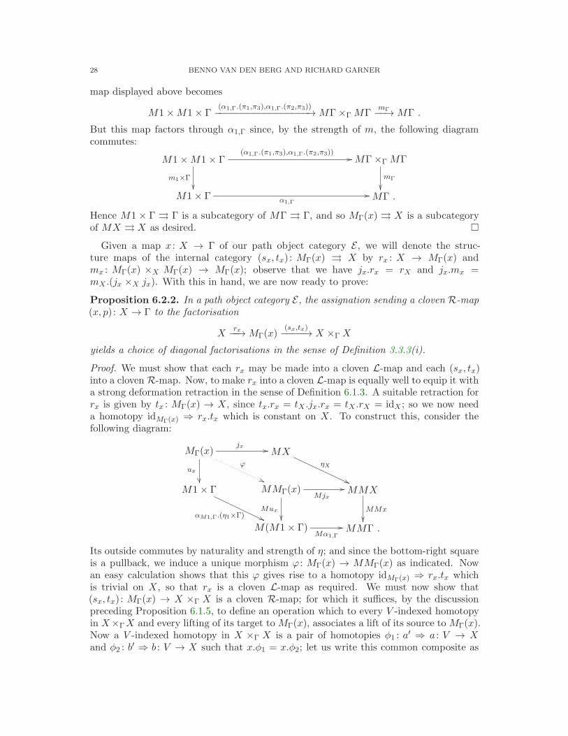
28 BENNO VAN DEN BERG AND RICHARD GARNER
map displayed above becomes
M1×M1× Γ(α1,Γ.(π1,π3),α1,Γ.(π2,π3))−−−−−−−−−−−−−−−−−→MΓ×Γ MΓ
mΓ−−→MΓ .
But this map factors through α1,Γ since, by the strength of m, the following diagramcommutes:
M1×M1× Γ(α1,Γ.(π1,π3),α1,Γ.(π2,π3))
m1×Γ
MΓ×Γ MΓ
mΓ
M1× Γ α1,ΓMΓ .
Hence M1 × Γ ⇒ Γ is a subcategory of MΓ ⇒ Γ, and so MΓ(x) ⇒ X is a subcategoryof MX ⇒ X as desired. �
Given a map x : X → Γ of our path object category E , we will denote the struc-ture maps of the internal category (sx, tx) : MΓ(x) ⇒ X by rx : X → MΓ(x) andmx : MΓ(x) ×X MΓ(x) → MΓ(x); observe that we have jx.rx = rX and jx.mx =mX .(jx ×X jx). With this in hand, we are now ready to prove:
Proposition 6.2.2. In a path object category E, the assignation sending a cloven R-map(x, p) : X → Γ to the factorisation
Xrx−−→MΓ(x)
(sx,tx)−−−−→ X ×Γ X
yields a choice of diagonal factorisations in the sense of Definition 3.3.3(i).
Proof. We must show that each rx may be made into a cloven L-map and each (sx, tx)into a cloven R-map. Now, to make rx into a cloven L-map is equally well to equip it witha strong deformation retraction in the sense of Definition 6.1.3. A suitable retraction forrx is given by tx : MΓ(x) → X, since tx.rx = tX .jx.rx = tX .rX = idX ; so we now needa homotopy idMΓ(x) ⇒ rx.tx which is constant on X. To construct this, consider thefollowing diagram:
MΓ(x)jx
uxϕ
MXηX
M1× Γ
αM1,Γ.(η1×Γ)
MMΓ(x)Mjx
Mux
MMX
MMx
M(M1× Γ)Mα1,Γ
MMΓ .
Its outside commutes by naturality and strength of η; and since the bottom-right squareis a pullback, we induce a unique morphism ϕ : MΓ(x) → MMΓ(x) as indicated. Nowan easy calculation shows that this ϕ gives rise to a homotopy idMΓ(x) ⇒ rx.tx whichis trivial on X, so that rx is a cloven L-map as required. We must now show that(sx, tx) : MΓ(x) → X ×Γ X is a cloven R-map; for which it suffices, by the discussionpreceding Proposition 6.1.5, to define an operation which to every V -indexed homotopyin X×ΓX and every lifting of its target toMΓ(x), associates a lift of its source toMΓ(x).Now a V -indexed homotopy in X ×Γ X is a pair of homotopies φ1 : a
′ ⇒ a : V → Xand φ2 : b
′ ⇒ b : V → X such that x.φ1 = x.φ2; let us write this common composite as

TOPOLOGICAL AND SIMPLICIAL MODELS OF IDENTITY TYPES 29
ψ : c′ ⇒ c : V → Γ. The target of (φ1, φ2) is the pair (a, b); and to give a lifting of this toMΓ(x) is to give a homotopy χ : a ⇒ b : V → X such that x.χ is a constant homotopyc ⇒ c; that is, one for which the corresponding map V → MΓ factors through M1 × Γ.From these data we are required to determine a homotopy χ′ : a′ ⇒ b′ : V → X for whichx.χ′ is a homotopy constant at c′. We may represent this diagrammatically as follows:
(27)
a′φ1
χ′
a
χ X
xb′
φ2b
c′ψ
c Γ .
We will construct χ′ as the composite of three homotopies constant over c′ which weobtain by means of the following two lemmas. The first describes a “cartesianness”property of the path-liftings obtained from a cloven R-map.
Lemma 6.2.3. Let (x, p) : X → Γ be a cloven R-map. Then to each V ∈ E and homotopy
ξ : y ⇒ z : V → X we may associate a homotopy ξ : y ⇒ (x.ξ)∗(z) constant over xy, such
that for all f : W → V we have ξf = ξ.f , and such that when ξ is an identity homotopy,so is ξ.
The second describes a “functoriality” property of these same path-liftings.
Lemma 6.2.4. Let (x, p) : X → Γ be a cloven R-map. Then to each V ∈ E, eachhomotopy ψ : c′ ⇒ c : V → Γ, and each homotopy ξ : y ⇒ z : V → X constant over c, wemay associate a homotopy ψ∗(ξ) : ψ∗(y) ⇒ ψ∗(z) : V → X constant over c′, in such away that for all f : W → V we have (ψf)∗(ξf) = (ψ∗(ξ)).f and such that when ψ is anidentity homotopy, ψ∗(ξ) = ξ.
If we leave aside the proof of these two lemmas for a moment, then we may constructχ′ as the composite homotopy
a′φ1==⇒ ψ∗(a)
ψ∗(χ)====⇒ ψ∗(b)
(φ2)◦====⇒ b′ .
Observe that this is a composite of homotopies constant over c′, and hence by Proposi-tion 6.2.1, is itself a homotopy constant over c′. In order to conclude that this assignationyields a cloven R-map structure on (sx, tx), we must verify two things. Firstly, that theoperation χ 7→ χ′ is natural in V—which follows immediately from the correspondingnaturalities noted in Lemmas 6.2.3 and 6.2.4—and secondly, that when φ1 and φ2 areidentity homotopies, we have χ′ = χ. But in this situation the displayed compositereduces, again by Lemmas 6.2.3 and 6.2.4, to the composite
a1a==⇒ a
χ=⇒ b
1b==⇒ b ,
which by left and right unitality of composition, is equal to χ. Note that, as anticipatedin Remark 4.3.3, this is the only point in the whole argument where we make use of theright unitality of composition. �
It remains to give the proof of the above two Lemmas.

30 BENNO VAN DEN BERG AND RICHARD GARNER
of Lemma 6.2.3. By the Yoneda lemma, to give the indicated assignation is equally wellto give a morphism δ : MX →MΓ(x) such that:
(28) sx.δ = sX , tx.δ = p.ξ, and δ.rX = rx,
where ξ : MX → Px is the morphism induced by the universal property of pullback inthe following diagram:
MXMx
tX
ξ
Pxdx
ex
MΓ
tΓ
X x Γ .
Now, postcomposition with p.ξ : MX → X takes a homotopy ψ : z ⇒ w : V → X andsends it to (x.ψ)∗(w) : V → X. In particular, when ψ is the identity homotopy on z,applying p.ξ gives back z again. Therefore we can construct the required homotopyz ⇒ (fψ)∗(w) by first forming the following “path of paths”
z
rX(z)
z
ψ
z w
in MMX using η and the involution τ , and then applying M(p.ξ) to it. Formally, weconsider the following composite:
MXτX−−→MX
ηX−−→MMXττX−−−→MMX
Mξ−−→MPx
Mp−−→MX .
We claim that this factors through the subobjectMΓ(x) of MX, so that we may define δto be the factorising map. To prove the claim, we must show that Mx.δ factors throughα1,Γ, for which we calculate that
Mx.δ =Mρx.Mξ.ττX .ηX .τX =MsΓ.MMx.ττX .ηX .τX
=Mx.MsX .ττX .ηX .τX =Mx.τX .MtX .ηX .τX
=Mx.τX .α1,X .(M !, tX ).τX =Mx.α1,X .(τ1.M !, tX).τX
= α1,Γ.(τ1.M !, x.tX ).τX
as required. It is now straightforward to check that this δ satisfies the equations in (28).�
of Lemma 6.2.4. Recall that, given a homotopy ψ : c′ ⇒ c : V → Γ and a homotopyξ : y ⇒ z : V → X constant over c, we are required to produce a homotopy ψ∗(ξ) : ψ∗(y) →ψ∗(z) constant over c′. We shall do so by first defining a homotopy θ : u ⇒ v : V → Pxwhich we schematically depict as:
(29) u =
c
ψ
xy
constant
xξ
c
ψ
xz
= v .

TOPOLOGICAL AND SIMPLICIAL MODELS OF IDENTITY TYPES 31
Thus u will correspond to the map V → Px picking out the homotopy ψ together withthe lifting y of its endpoint, whilst v will correspond to the map picking out ψ togetherwith the lifting z of its endpoint. It follows that postcomposing θ with p : Px→ X yieldsthe desired homotopy ψ∗(ξ) : ψ∗(y) ⇒ ψ∗(z) : V → X.
Now, to give the homotopy θ is to give a map V → MPx which—since M preservespullbacks—is equally well to give maps γ and δ rendering commutative the square
(30)
Vδ
γ
MMΓ
MtΓ
MXMx
MΓ .
To define γ and δ, let us first note that to give the homotopies ψ and ξ is equally wellto give maps—which by abuse of notation, we also denote by ψ and ξ—rendering thefollowing square commutative:
Vψ
ξ
MΓ
tΓ
MΓ(x) π2.uxΓ .
Now by referring to our schematic depiction (29), we see that we should take γ = jx.ξ,and take δ to be the composite
V(π1.ux.ξ, ψ)−−−−−−−→M1×MΓ
α1,MΓ−−−−→MMΓ
picking out the homotopy inMΓ “constant at ψ and of the same length as ξ”. We now cal-culate thatMtΓ.δ =MtΓ.α1,MΓ.(π1.ux.ξ, ψ) = α1,Γ.(π1.ux.ξ, tΓ.ψ) = α1,Γ.(π1.ux.ξ, π2.ux.ξ) =α1,Γ.ux.ξ =Mx.jx.ξ =Mx.γ, so that (30) commutes; and thus we have an induced mor-phism (γ, δ) : V → MPx defining the desired homotopy θ : u⇒ v : V → Px. Observethat u and v are the morphisms V → Px induced by the universal property of pullbackin the respective diagrams
VsMΓ.δ
sX .γ
MΓ
tΓ
X x Γ
and
VtMΓ.δ
tX .γ
MΓ
tΓ
X x Γ
;
and we calculate that sMΓ.δ = sMΓ.α1,MΓ.(π1.ux.ξ, ψ) = π2.(π1.ux.ξ, ψ) = ψ and thatsX .γ = sX .jx.ξ = sx.ξ = y; similarly that tMΓ.δ = ψ and that tX .γ = z. Hence if wedefine ψ∗(ξ) to be the compositeMp.θ, then we obtain a homotopy ψ∗(y) ⇒ ψ∗(z) : V →X as required. It remains to check three things. Firstly, we must show that ψ∗(ξ) isa constant homotopy; it will then necessarily be over c′, since ψ∗(y) and ψ∗(z) are.For this, we must show that the composite morphism Mx.Mp.(γ, δ) : V → MΓ factorsthrough α1,Γ; and so we calculate that Mx.Mp.(γ, δ) =Mρx.(γ, δ) =MsΓ.Mdx.(γ, δ) =MsΓ.δ =MsΓ.α1,MΓ.(π1.ux.ξ, ψ) = α1,Γ.(π1.ux.ξ, sΓ.ψ) as required.
Secondly, we must show that for any f : W → V , we have (ψf)∗(ξf) = (ψ∗(ξ))f . Thisis immediate by the universal property of pullback. Finally, we must show that when ψ

32 BENNO VAN DEN BERG AND RICHARD GARNER
is an identity homotopy, we have ψ∗(ξ) = ξ. In this case, we have that ψ = rΓ.tΓ.ψ : V →MΓ; and are required to show that Mp.(γ, δ) = jx.ξ : V →MX. We calculate that
δ = α1,MΓ.(π1.ux.ξ, ψ) = α1,MΓ.(π1.ux.ξ, rΓ.tΓ.ψ) = α1,MΓ.(π1.ux.ξ, rΓ.π2.ux.ξ)
=MrΓ.α1,Γ.(π1.ux.ξ, π2.ux.ξ) =MrΓ.α1,Γ.ux.ξ =MrΓ.Mx.jx.ξ ,
and so have that Mp.(γ, δ) = Mp.(idMX ,MrΓ.Mx).jx.ξ = Mp.Mλx.jx.ξ = jx.ξ asrequired. �
This completes the proof of the two Lemmas, and hence of Proposition 6.2.2. So wehave established the existence of a choice of diagonal factorisations for the cloven w.f.s.associated to any path object category; the crucial point is that this choice is a suitablywell-behaved one.
Proposition 6.2.5. For any path object category E, the choice of diagonal factorisationson its associated cloven w.f.s. given by Proposition 6.2.2 is functorial and stable in thesense of Definition 3.3.3(ii)–(iii).
Proof. To show functoriality, observe first that if E is a path object category, and Cany category, then the functor category [C, E ] becomes a path object category with thestructure given pointwise; and that the category of R-maps in [C, E ] is then [C,R-MapE ],and correspondingly for the category of L-maps. In particular, given any path objectcategory E , the path object category [R-MapE , E ] contains a “generic R-map”, corre-sponding to the identity functor R-MapE → R-MapE . Applying Proposition 6.2.2 tothis generic R-map yields the desired functoriality.
It remains to show stability: for which it suffices to show that, given a cloven R-mapx : X → Γ together with a morphism f : ∆ → Γ, there is an isomorphism f∗(MΓ(x)) →M∆(f
∗x) over ∆ which is compatible with r, s and t in the obvious way. Now, f∗(MΓ(x))is isomorphic to the composite down the left of the following diagram, all of whose squaresare pullbacks:
f∗(MΓ(x)) MΓ(x)jx
ux
MX
Mx
M1×∆M1×f
π2
M1× Γ α1,Γ
π2
MΓ .
∆f
Γ
On the other hand, M∆(f∗x) is obtained as the composite with π2 of the arrow down
the left of the following diagram, all of whose squares are again pullbacks
M∆(f∗X) M(f∗X)
M(f∗x)
MX
Mx
M1×∆ α1,∆M∆
MfMΓ .
But since Mf.α1,∆ = α1,Γ.(M1 × f) by naturality of α, we have these two compositesisomorphic to each other over ∆ as required. The naturality of these isomorphisms, andtheir coherence with the remaining data, is easily checked. �

TOPOLOGICAL AND SIMPLICIAL MODELS OF IDENTITY TYPES 33
6.3. Functorial Frobenius structure. We have now verified that any path objectcategory can be equipped with a cloven w.f.s. which has a stable functorial choice ofdiagonal factorisations. The final step in proving Theorem 4.3.2 is to show that thiscloven w.f.s. is functorially Frobenius.
Proposition 6.3.1. If E is a path object category, then its associated cloven w.f.s. isfunctorially Frobenius in the sense of Definition 3.3.3(iv).
Proof. Let (f, p) : B → A be a cloven R-map and (i, q) : X → A a cloven L-map in E ,and consider a pullback square
f∗Xf
ı
X
i
Bf
A .
We are required to equip ı with the structure of a cloven L-map. Recall from The-orem 6.1.4 that to give a cloven L-map structure on i is to give a strong deforma-tion retraction for it: thus a map k : A → X satisfying ki = idX and a homotopyθ : 1A ⇒ ik : A → A such that θ.i = 1i : i ⇒ i. Correspondingly, to construct a clovenL-map structure on ı it suffices to give a strong deformation retraction for it. So con-sider the homotopy φ = (θf)◦ : ikf ⇒ f : B → A, where we recall from Remark 6.1.1that (–)◦ is the reversal operation on homotopies induced by τ . Since f is a clovenR-map, we may apply its path-lifting property, described in Proposition 6.1.5, to obtainfrom this a morphism φ∗(1B) : B → B and a homotopy φ : φ∗(1B) ⇒ 1B : B → B suchthat f.φ = φ. In particular, this means that f.φ∗(1B) = ikf , and so we may induce amorphism k : B → f∗X by the universal property of pullback in
Bkf
φ∗(1B)
k
f∗Xf
ı
X
i
Bf
A .
Now taking θ = (φ)◦ : 1B ⇒ ık, then it remains to show that k.ı = 1f∗B and that θ.ı isthe identity homotopy on ı. Firstly, to show that k.ı = 1f∗B , it suffices to demonstrateequality on postcomposition with f and with ı. On the one hand, we have that f .k.ı =k.f.ı = k.i.f = f ; whilst on the other, we have ı.k.ı = φ∗(1B).ı = (φ.ı)∗(ı) by naturalityof the liftings described in Proposition 6.1.5. But φ.ı = (θf)◦.ı = (θf ı)◦ = (θif)◦ =(1if )
◦ = 1if , and so by Proposition 6.1.5 again we have (φ.ı)∗(ı) = ı as required. Thus
k.ı = 1f∗B, and it remains only to show that θ.ı = 1ı. Applying (–)◦ to both sides, itsuffices to show that φ.ı = 1ı. But by naturality of the liftings of Proposition 6.1.5, wehave φ.ı = φ.ı, and since φ.ı is an identity homotopy as above, we deduce that φ.ı is aswell.
Thus we have equipped ı with the structure of a strong deformation retract, and henceof a cloven L-map, which completes the verification that the cloven w.f.s. associated to

34 BENNO VAN DEN BERG AND RICHARD GARNER
E is Frobenius. Finally, to show that it is functorially Frobenius we apply an entirelyanalogous argument to that given in Proposition 6.2.5. �
This now completes the proof of Theorem 4.3.2.
7. The simplicial path object category
In this final section, we fill in the details of the proof, sketched in Section 5.5, thatsimplicial sets form a path object category. We begin by establishing some notationalconventions. Recall that ∆ is the category whose objects are the ordered sets [n] ={0, . . . , n} (for n ∈ N) and whose morphisms are order-preserving maps, and that thecategory SSet of simplicial sets is the presheaf category [∆op,Set]. As before, we writeXn := X([n]) for the set of n-simplices of a simplicial set X; and given an element x ∈ Xn
and a map α : [m] → [n], we shall write x · α for X(α)(x) ∈ Xm. We refer to maps of∆ as simplicial operators, and call monomorphisms face operators and epimorphismsdegeneracy operators. Of particular note are the operators δi : [n− 1] → [n] and σi : [n+1] → [n] (for 0 6 i 6 n) defined as follows: δi is the unique monomorphism [n− 1] → [n]whose image omits i; whilst σi is the unique epimorphism [n + 1] → [n] whose imagerepeats i. The maps δi and σi generate the category ∆ under composition, though notfreely; they obey the following simplicial identities, describing how faces and degeneraciescommute past each other:
δjδi = δiδj−1 for i < j
σjσi = σiσj+1 for i 6 jσjδi =
δiσj−1 for i < j
id for i = j, j + 1
δi−1σj for i > j + 1.
7.1. Path objects. Our first task is to describe the construction assigning to each sim-plicial set X the simplicial set of Moore paths in X. We begin by making precise theinformal description of n-dimensional Moore paths given in Section 5.5.
Definition 7.1.1. Let X be a simplicial set and let ξ, ξ′ be n-simplices in X. An n-dimensional Moore path from ξ to ξ′ is given by n-simplices ξ = ζ0, . . . , ζk = ξ′ and(n+ 1)-simplices φ1, . . . , φk, together with a function
(31) θ : {1, . . . , k} → [n]× {+,−}
such that
(32) ζi−1 =
{φi · δm+1 if θ(i) = (m,+)
φi · δm if θ(i) = (m,−)ζi =
{φi · δm if θ(i) = (m,+)
φi · δm+1 if θ(i) = (m,−) .
We call functions like (31) n-dimensional traversals; the natural number k will becalled the length of the traversal. In order to explain the role which such traversals play,we consider once again the example of a 1-dimensional Moore path from (23) above:
xf1
ξ ζ1 ζ2
z1f2
ζ3
z2
ζ4
z3f3
ζ5 ζ6
f4
φ7
z4
ζ7
φ8
y .f5
ξ′
x′f ′1
φ1
z′1
φ2
φ3 φ4
z′2f ′2 f ′3
y′
φ5
φ6

TOPOLOGICAL AND SIMPLICIAL MODELS OF IDENTITY TYPES 35
The intuition is that each 2-simplex φi appearing in it is so oriented that it may be“projected” in an orientation-preserving manner onto ξ. Under this projection, preciselyone edge of φi will be collapsed; and the value of θ(i) indicates at which vertex of ξ thiscollapsing occurs, and in which direction the collapsed edge points. Thus, for the aboveexample, the values of the traversal θ are given by the list
(1,+), (1,−), (0,+), (0,+), (0,−), (1,+), (0,+), (0,−) .
Observe that the face equations of (32) enforce the discipline that makes this intuitionprecise.
Proposition 7.1.2. There is a simplicial setMX whose n-simplices are the n-dimensionalMoore paths in X.
To prove this Proposition, we must describe a coherent action by simplicial operatorson the simplices ofMX. The basic idea may be illustrated with reference to the examplesof Moore paths given above. In the case of a 1-dimensional Moore path like (23), its two0-dimensional faces should be obtained by projection on to the top and bottom rows ofthe diagram; whilst in the case of a 0-dimensional Moore path like (22), its image underthe degeneracy σ0 : [1] → [0] will be the 1-dimensional Moore path
xf1
x·σ0 f1
z1f2
z1·σ0 f2
z2
z2·σ0
z3f3 f4
z3·σ0f3 f4
z4
z4·σ0
x′f5
x′·σ0f5
xf1
f1·σ0
f1·σ1
z1f2
f2·σ0
f2·σ1
z2 z3f3 f4
f4·σ0
f4·σ1
f3·σ0
f3·σ1
z4 x′ .f5
f5·σ0
f5·σ1
In giving a formal proof of Proposition 7.1.2, it will be convenient to consider firstthe special case where X = 1, the terminal simplicial set. Observe that the n-simplicesof M1 are simply n-dimensional traversals. Given such a traversal θ of length k and asimplicial operator α : [m] → [n], it is easy to see that there is a unique pullback diagram
(33)
{1, . . . , ℓ}ψ
α
[m]× {+,−}
α×{+,−}
{1, . . . , k}θ
[n]× {+,−}
such that the following condition is satisfied:
(†)
α is order-preserving, and for i ∈ {1, . . . , k}, the restrictionof ψ to the fibre of α over i is order-reversing if θ(i) = (x,+)for some x, and order-preserving if θ(i) = (x,−).
We may therefore define θ ·α ∈ (M1)m to be ψ. It is immediate that θ · idm = θ, and it’seasy to check that pullback squares satisfying (†) are stable under composition, so thatθ · (αβ) = (θ · α) · β. Thus M1 is a simplicial set as required; and we now exploit thisfact in proving the same for a general MX. The key observation we will make is that atypical n-simplex of MX is given by an n-simplex of M1 that has been suitably labelledwith simplices of X. To make this precise, we first need:

36 BENNO VAN DEN BERG AND RICHARD GARNER
Notation 7.1.3. Given a traversal θ, we write
θ+(i) =
{x if θ(i) = (x,+)
x+ 1 if θ(i) = (x,−)and θ−(i) =
{x+ 1 if θ(i) = (x,+)x if θ(i) = (x,−)
Also, in circumstances where it cannot cause confusion, we may choose to write the xsuch that θ(i) = (x, ρ) simply as θ(i).
In terms of this notation, to give an n-simplex of MX is to give a traversal θ ∈ (M1)nof length k together with n-simplices ζ0, . . . , ζk and (n + 1)-simplices φ1, . . . , φk suchthat for each 1 6 i 6 k, we have ζi−1 = φi · δθ−i and ζi = φi · δθ+i. We may further recastthis description by means of the following definition.
Definition 7.1.4. If θ : {1, . . . , k} → [n] × {+,−} is a traversal, then its simplicial
realisation is the simplicial set θ obtained as the colimit of the diagram
(34) Dθ :=
[n]
δθ−(1)
[n]
δθ+(1) δθ−(2)
. . .
δθ+(2) δθ−(k)
[n]
δθ+(k)
[n+ 1] [n+ 1] [n+ 1]
of simplicial sets, wherein we identify objects and morphisms of ∆ with their imagesunder the Yoneda embedding ∆ → [∆op,Set]. We write sθ, tθ : [n] → θ for the colimitinjections from the leftmost and rightmost copies of [n].
Using this definition we see that an n-simplex of MX may be identified with a pair(θ, φ) where θ is an n-simplex of M1 and φ : θ → X. Consequently, to equip MX withthe structure of a simplicial set, it suffices to prove:
Proposition 7.1.5. To every simplicial operator α : [m] → [n] and traversal θ we may
assign a map of simplicial sets α : θ · α → θ. Moreover, this assignment is functorial in
the sense that 1[n] = 1θand β ◦ α = β ◦ α.
Indeed, given this result we may define an action of the simplicial operator α : [m] → [n]on an n-simplex (θ, φ) ofMX by (θ, φ) ·α = (θ ·α, φ◦α); with the coherence equations forthis action following easily from the functoriality in Proposition 7.1.5. Thus to completethe proof that MX is a simplicial set, it remains only to give:
of Proposition 7.1.5. Suppose that θ : {1, . . . , k} → [n]×{+,−}, and let us write ψ : {1, . . . , ℓ} →[m]×{+,−} for the traversal θ ·α; recall that it is defined as the unique function fittinginto a pullback square of the form (33). For each 1 6 j 6 k, we define ψi to be thetraversal given by restricting ψ to the fibre α−1(i) ⊂ {1, . . . , ℓ} (and renumbering, since
the smallest element of this fibre is probably not 1). Then to give a morphism ψ → θ, itsuffices to find maps f1, . . . , fk rendering commutative the diagram
(35)
[m]
αsψ1
[m]tψ1 sψ2
α
. . .tψ2 sψk
[m]tψk
α
[n]
δθ−(1)
ψ1
f1
[n]
δθ+(1) δθ−(2)
ψ2
f2
. . .
δθ+(2) δθ−(k)
ψk
fk
[n] ,
δθ+(k)
[n+ 1] [n+ 1] [n+ 1]

TOPOLOGICAL AND SIMPLICIAL MODELS OF IDENTITY TYPES 37
since ψ and θ are the respective colimits of the upper and lower zigzags in this diagram.In fact, we claim that there is a unique way of choosing the fi’s given the remainingdata: which as well as proving the existence of α, easily implies the functoriality in α.It remains to prove the claim. So let 1 6 i 6 k, and assume that θ(i) = (a,−) forsome 0 6 a 6 n: something we may do without loss of generality, since the case whereθ(i) = (a,+) is entirely dual. We first consider the situation in which a is not in the
image of α. In this case, we have that ψi = [m] and sψi = tψi = 1[m], so that fi isnecessarily unique, and will exist so long as the square
[m]α α
[n]
δa
[n]
δa+1
[n+ 1]
commutes: which it does since a is not in the image of α. Turning now to the case wherea is in the image of α, we observe that α−1(a) is a non-empty segment of [m], and sowriting p and q for its smallest and largest elements, we have by virtue of the condition(†) defining ψ that ψi is the traversal of length q − p+ 1 given by ψi(x) = (p+ x− 1,−);so that to give fi is equally well to give the dotted maps in
(36)
[m]δp
hp:=δaα
[m]δp+1 δp+1
hp+1
. . .δp+2 δq
[m] .δq+1
hq+1:=δa+1α
[m+ 1]
gp
[m+ 1]
gp+1
[m+ 1]
gq
[n+ 1]
We wish to show that there is a unique way of doing this. Note first that if such mapsexist, then commutativity in
[m− 1]δp δp
[m]
δp
[m]
δp+1
[m+ 1]
implies that hp.δp = hp+1.δp; in other words, that hp and hp+1 are the same, exceptpossibly for their value at p. More generally, we see that for each p 6 j 6 q, the mapshj and hj+1 agree everywhere except possibly at j. It follows that a typical hj mustagree with hp at all values except for those in {p, . . . , j − 1}, and must agree with hq+1
at all values except for those in {j, . . . , q}. Since hp and hq+1 agree at all values except{p, . . . , q}, this is certainly possible, and forces the definition
(37) hj(x) :=
{hq+1(x) for x < j ;
hp(x) for x > j ,i.e., hj(x) :=
{α(x) for x < j ;
α(x) + 1 for x > j .

38 BENNO VAN DEN BERG AND RICHARD GARNER
Now since gj .δj = hj and gj .δj+1 = hj+1, it is easy to see that this in turn forces thedefinition
(38) gj(x) :=
{α(x) for x 6 j ;
α(x− 1) + 1 for x > j .
Thus we have shown that there a unique way of filling in the dotted arrows in (36), andhence also a unique way of filling in the dotted arrows in (35): which completes theconstruction of the desired map α, and also implies the functoriality of the constructionin α. �
7.2. First axiom. We have now completed the construction of the simplicial set MXof Moore paths in X. Recall that we did so by making use of the isomorphism
(39) (MX)n ∼=∑
θ∈(M1)n
SSet(θ, X)
to define the action of a simplicial operator α : [m] → [n] on an n-simplex (θ, φ) by(θ, φ) · α = (θ · α, φ ◦ α). We will exploit the isomorphism (39) further in proving that:
Proposition 7.2.1. The simplicial sets MX provide data for Axiom 1 of a path objectstructure on SSet.
Proof. Given a map f : X → Y of simplicial sets, we define the action of Mf on an n-simplex (θ, φ) by Mf(θ, φ) = (θ, fφ). It is immediate that this yields a map of simplicialsets MX → MY , functorially in f . To see that the functor M so defined preservespullbacks, observe that it suffices to do so componentwise; and that (39) expresses eachsuch component (M–)n as a coproduct of limit-preserving functors, and so as a pullback-(and indeed, connected limit-) preserving functor.
We define the maps sX , tX : MX → X by sending (θ, φ) ∈ (MX)n to the n-simplexclassified by the composites φ ◦ sθ and φ ◦ tθ : [n] → X (where sθ and tθ are as inDefinition 7.1.4). Commutativity in the extremal squares of (35) ensure that sX and tXare maps of simplicial sets. To define rX : X → MX, we note that the realisation ofthe empty n-dimensional traversal ǫ is simply [n], so that we may define rX(x) = (ǫ, x),where x : [n] → X is the map classifying x. Compatibility with the simplicial structureagain follows from (35).
To define the morphism mX : MX ×X MX →MX, observe that an n-simplex of thedomain of this map is given by elements (θ1, φ1) and (θ2, φ2) ∈ (MX)n with φ1 ◦ tθ1 =φ2 ◦ sθ2 . We take their composite to be (θ1 + θ2, ψ), where if θ1 and θ2 are traversals oflength k1 and k2 respectively, then θ1 + θ2 is the traversal of length k1 + k2 given by:
(θ1 + θ2)(x) =
{θ1(x) for 1 6 x 6 k1 ;
θ2(x− k1) for k1 < x 6 k1 + k2 .
To give ψ, we observe that we have a pushout square:
[n]tθ1 sθ2
θ1 θ2
θ1 + θ2

TOPOLOGICAL AND SIMPLICIAL MODELS OF IDENTITY TYPES 39
where the two unlabelled arrows are the canonical inclusions, so that we may take
ψ : θ1 + θ2 → X to be the map induced by the universal property of this pushout appliedto the pair φ1 : θ1 → X and φ2 : θ2 → X. Simpliciality of mX follows by observing thatits induced effect on diagrams of the form (35) is simply that of by placing them side byside.
It is easy to see that the data given so far equip MX ⇒ X with the structure ofan internal category, naturally in X; and so it remains only to provide the identity-on-objects involution τX : MX → MX. To do so, we first define the reverse of a traversalθ : {1, . . . , k} → [n]× {+,−}. This will be the traversal θo of length k given by
θo(x) =
{(y,+) if θ(k + 1− x) = (y,−);
(y,−) if θ(k + 1− x) = (y,+).
Now observe that there is a canonical isomorphism eθ : θo → θ, since the diagram Dθo
of which the latter is a colimit is obtained by laterally mirroring the diagram Dθ for theformer. We may therefore define the involution τX by sending the n-simplex (θ, φ) to(θo, φ ◦ eθ). Since eθo = e−1
θ , this operation is involutive, and is easily seen to respectthe category structure and to be natural in X. It remains to check that τX commuteswith the action of simplicial operators. Observe first that for any simplicial operatorα : [m] → [n], we have (θ · α)o = θo · α by virtue of the condition (†) in the definition ofthe action of α. Moreover, any diagram of the form
θ · αeθ·α
α
θo · α
α
θ eθ θo
will commute, since the effect of the operation (–)o on diagrams of the form (35) is tomirror them laterally. It follows from this that τX commutes with the action by simplicialoperators as required. �
7.3. Second axiom. We have now provided all the data for Axiom 1 of a path objectstructure on the category of simplicial sets; and so now turn to Axiom 2.
Proposition 7.3.1. The endofunctor M on simplicial sets defined in Proposition 7.3.1may be equipped with a strength which validates Axiom 2 for a path object category.
Proof. By the remarks made in Section 4.2, it suffices to provide components α1,X : M1×X →MX for the strength. To do this, we first define, for every n-dimensional traversalθ, a map jθ : θ → [n] induced by the cocone
(40)
[n]δθ−(1)
id
[n]δθ+(1) δθ−(2)
id
. . .δθ+(2) δθ−(k)
[n]δθ+(k)
id
[n+ 1]
σθ(1)
[n+ 1]
σθ(2)
[n+ 1]
σθ(k)
[n]

40 BENNO VAN DEN BERG AND RICHARD GARNER
under the diagram Dθ of which θ is a colimit. Now given an n-simplex (θ, x) of M1×X,we define its image under α1,X to be (θ, x ◦ jθ), where as before, x : [n] → X is the mapclassifying x. To show that this yields a map of simplicial sets, it is evidently enough toverify that diagrams of the form
θ · αjθ·α
α
[m]
α
θ jθ[n]
commute. Now since α is defined by the diagram (35), it suffices for this to show that,using the notation of that diagram, the square
ψijψi
fi
[m]
α
[n+ 1]σθ(i)
[n]
commutes for each i. Recalling that the morphism fi was defined by the diagram (36)—in which we have assumed, without loss of generality, that θ(i) = (a,−)—it thereforesuffices to show, using the notation of that diagram, that σa.gj = α.σj for each p 6 j 6 q:and this follows by direct examination of the equation (38) defining gj . This completesthe verification that α1,X is a map of simplicial sets; and it is straightforward to verifythat these maps are natural in X, and that the strength axioms are satisfied. Now thatr is strong follows by observing that jǫ = id[n] (where as before ǫ is the empty traversalof dimension n); that s and t are strong follows from the commutativity of the extremaltriangles in (40); that m is strong follows by noting that for n-dimensional traversals θ1and θ2, the following diagram commutes:
θ1
jθ1
θ1 + θ2
jθ1+θ2
θ2
jθ2
[n]
in which the horizontal arrows are the canonical inclusions; whilst that τ is strong followsfrom the fact that for any traversal θ, the diagram
θeθ
jθ
θo
jθo
[n]
commutes. �
7.4. Third axiom. The last part of the proof that simplicial sets form a path objectcategory will be to construct the maps ηX : MX →MMX which, to every n-dimensionalMoore path in X, associate an n-dimensional Moore path in MX which contracts the

TOPOLOGICAL AND SIMPLICIAL MODELS OF IDENTITY TYPES 41
given path on to its endpoint. We motivate the construction by considering the exam-ple (24) of Section 5.5 above, which demonstrates the action of ηX on the 0-dimensionalMoore path of (23). The first observation we can make about the Moore path of (24) isthat it has the same underlying traversal as the path (23) of which it is a contraction.So for a general n-dimensional Moore path x = (θ, φ) of length k in X, we aim to giveηX(x) of the form (θ, ηX(φ)) in MX. To do this, we must provide (k + 1) n-simplicesand k (n+ 1)-simplices of MX which are matched together in the fashion dictated by θ.To give the n-simplices is straightforward; as suggested by our example (24), these willbe obtained by suitably truncating the original path.
Definition 7.4.1. Let x = (θ, φ) be an n-dimensional Moore path of length k in X. For0 6 i 6 k, we define the tail at i to be the n-dimensional Moore path xi = (θi, φi) oflength k − i whose traversal is the function x 7→ θ(x+ i), and whose second componentis the composite
θi → θφ−→ X
in which the first arrow is the canonical inclusion.
It remains to define the (n+1)-simplices of MX that will mediate between the tail ati and the tail at i+ 1; and consideration of the example (24) suggests that these shouldbe obtained by first forming a suitable degeneracy of the tail at i, and then removing itsfirst element. For example, looking at the case i = 1 in (24), we see that we have:
z1 f1
z2·σ0f1
z2
z2·σ0
z3f2 f3
f2 z3·σ0 f3
z4
z4·σ0
x′f4
f4x′·σ0
z1 f1 z2 z3f2 f3 z4 x′ ,f4
which has been obtained by removing the first element from the degeneracy σ0 of thetail at 1. This motivates the following definition:
Definition 7.4.2. Let x = (θ, φ) be an n-dimensional Moore path of length k in X. Wedefine ηX(x) to be the n-dimensional Moore path inMX whose traversal is θ, and whose
second component ηX(φ) : θ →MX is the map induced by the cocone
(41)
[n]δθ−(1)
x0
[n]δθ+(1) δ
θ−(2)
x1
. . .δθ+(2) δ
θ−(k)
[n] .δθ+(k)
xk
[n+ 1]
(x0·σθ(1))1
[n+ 1]
(x1·σθ(2))1
[n+ 1]
(xk−1·σθ(k))1
MX
In order for this definition to make sense, we must verify that the diagram (41) ap-pearing in it is commutative. We do so using the following result.
Lemma 7.4.3. Let x = (θ, φ) be an n-dimensional Moore path of length k, and letα : [m] → [n] be a simplicial operator. Then for any 0 6 i 6 k, we have xi · α = (x · α)ı,
where ı =∑i
j=1
∣∣α−1(θ(j))∣∣.

42 BENNO VAN DEN BERG AND RICHARD GARNER
Proof. Observe that as well as xi, the tail at i, we may also by duality form xi, the headat i: we take xi := ((xo)k−i)o. It is now easy to see that x = mX(x
i, xi); and moreover,that if x = mX(z, y) with y of length i, then necessarily y = xi and z = xi. Now we havethat x · α = mX(x
i, xi) · α = mX(xi · α, xi · α) and hence that xi · α = (x · α)ı, where ı is
the length of xi · α. But examination of the pullback square (33) shows that this length
is∑i
j=1
∣∣α−1(θ(j))∣∣ as required. �
We now show commutativity in (41). For 1 6 i 6 k, we have by condition (†) onpage 35 that the first element of the traversal associated with xi−1 · σθ(i) is of the form
(θ−(i), ρ): and so by the preceding Lemma, we obtain
(42)(xi−1 · σθ(i))
1 · δθ−(i) = (xi−1 · σθ(i) · δθ−(i))0 = xi−1
and (xi−1 · σθ(i))1 · δθ+(i) = (xi−1 · σθ(i) · δθ+(i))
1 = (xi−1)1 = xi .
Proposition 7.4.4. The assignation x 7→ ηX(x) of Definition 7.4.2 provides data foran instance of Axiom 3 for a path object structure on the category of simplicial sets.
Proof. The hardest part of the proof will be to verify that ηX is a map of simplicialsets. Given x ∈ (MX)n and a simplicial operator α : [m] → [n], we must show thatηX(x · α) = ηX(x) · α. Suppose that x = (θ, φ) is a traversal of length k, and writeψ = θ · α. Then to verify that ηX(x · α) = ηX(x) · α it suffices to show that for each1 6 i 6 k, the square
(43)
ψi
fi
ψ
ηX(x·α)
[n+ 1](xi−1·σθ(i))
1MX
commutes, where fi and ψi are as defined in (35), and where the unlabelled horizontalmap is the evident inclusion. So let us fix some 1 6 i 6 k, and suppose without loss ofgenerality that θ(i) = (a,−). Let us also define r =
∑i−1j=1
∣∣α−1(θ(j))∣∣, and observe that
with this definition, the canonical inclusion ψi → ψ maps the jth m- or (m+ 1)-simplex
of ψi to the (j + r)th m- or (m+1)-simplex of ψ. To prove that (43) commutes, we firstconsider the degenerate case where ψi is an empty traversal: that is, when a is not inthe image of α. Then by the proof of Proposition 7.1.5, we have ψi = [m] and fi = δaα,so that we must verify that the diagram
[m]
δaα(x·α)r
[n+ 1](xi−1·σa)1
MX
commutes. But by (42) and Lemma 7.4.3 we have (xi−1 · σa)1 · δa ·α = xi−1 ·α = (x ·α)r
as required. Suppose now that ψi is a non-empty traversal, given as in the proof ofProposition 7.1.5 by the function ψi(x) = (p + x − 1,−). Now to show commutativityin (43), it suffices to do so on precomposition with the q − p + 1 colimit injections
[m + 1] → ψi. If we label these injections with natural numbers p 6 j 6 q, then

TOPOLOGICAL AND SIMPLICIAL MODELS OF IDENTITY TYPES 43
precomposing (43) with the jth one yields the diagram
(44)
[m+ 1]
gj((x·α)j+r−p·σj)
1
[n+ 1](xi−1·σa)1
MX .
Now the first element of the traversal associated with (xi−1 · σa) is (a,−); and hence by
Lemma 7.4.3, we have (xi−1 · σa)1 · gj = (xi−1 · σa · gj)
|g−1j (a)|. But by direct examination
of (38), we see that |g−1j (a)| = j − p+1; moreover, we have as above that xi−1 · σa · gj =
xi−1 · α · σj = (x · α)r · σj, and so conclude that the map along the lower side of (44) isequal to (xi−1 · σa)
1 · gj = ((x · α)r · σj)j−p+1. Now, along the upper side we have ((x ·
α)j+r−p ·σj)1 = (((x·α)r)j−p ·σj)
1 = ((x·α)r ·σj)ı+1, where here ı =
∑j−ph=1 |σ
−1j (ψ(h+r))|.
To prove equality in (44), it therefore suffices to show that ı = j − p. But we have that
ψ(h+ r) = ψi(h) = p+h− 1 so that ı =∑j−p
h=1 |σ−1j (p+h− 1)| = j− p as required. This
proves that (44), and hence (43), are commutative, which completes the verification thatηX is a map of simplicial sets. It is now straightforward to verify that the ηX ’s so definedare natural in X and strong; and so it remains only to check the equations (16)–(20).
For equations (16) and (17), it is immediate from (41) that sMX(ηX(x)) = x0 = x andthat tMX(ηX(x)) = xk = rX(tX(x)) as required, whilst for equation (20), we calculatethat ηX(rX(x)) = ηX(ǫ, x) = (ǫ, (ǫ, x)) = rMX(rX(x)) as required. Thus it remainsto verify equations (18) and (19), which, we recall, say that MsX .ηX = idMX andMtX .ηX = α1,X .(M !, tX ). Now, given an n-simplex x = (θ, φ) of X we have thatMsx(ηX(x)) andMtX(ηX(x)) are given by the simplices (θ, sX .ηX(φ)) and (θ, tX .ηX(φ))respectively, and that α1,X .(M !, tX) is given by the simplex (θ, tX(x).jθ), where jθ is asdefined in Proposition 7.3.1. Thus to verify equations (18) and (19), we must prove that
sX .ηX(φ) = φ and tX .ηX(φ) = tX(x).jθ
as maps θ → X. But since θ is the colimit of the diagram (34), it suffices to show these two
equalities on precomposition with the each of the colimit injections q1, . . . , qk : [n+1] → θ.The latter case is simpler: we calculate that
tX .ηX(φ).qi = tX .((xi−1 · σθ(i))
1) = tX .(xi−1 · σθ(i))
= tX(xi−1) · σθ(i) = tX(x).σθ(i) = tX(x).jθ.qi
as required. For the former case, we must show that sX((xi−1 · σθ(i))
1) = φ.qi as maps[n + 1] → X. For definiteness, let us suppose that θ(i) = (a,−); the case where it is(a,+) is entirely dual. Now sX((x
i−1 · σθ(i))1) is the composite
(45) [n+ 1]u−→ θi−1 · σa
σa−−→ θi−1 → θφ−→ X
in which the first arrow u picks out the second copy of [n + 1] in the colimit definingits codomain. In order to simplify this composite further, consider the morphism σaappearing in it. This is induced by a diagram of the form (35), whose left-hand edge is

44 BENNO VAN DEN BERG AND RICHARD GARNER
given by
[n+ 1]
σaδa
[n+ 1]δa+1 δa+1
ha+1
[n+ 1]
σaδa+2
[n]
δa
[n+ 2]
ga
[n+ 2]
ga+1
[n]
δa+1
. . .
[n+ 1]
where the dotted arrows are defined as in (36). In particular, by inspection of (37), wesee that ha+1 is the identity. Hence the composite σau is the morphism picking out the
leftmost [n + 1]-simplex in the colimit defining θi−1, and hence (45) is equal to φ.qi asrequired. �
This completes the verification of Axiom 3, and hence of:
Proposition 7.4.5. The category of simplicial sets bears the structure of a path objectcategory.
References
[1] Awodey, S., and Warren, M. Homotopy theoretic models of identity types. Mathematical Pro-ceedings of the Cambridge Philosophical Society 146, 1 (2009), 45–55. 1, 7
[2] Bousfield, A. Constructions of factorization systems in categories. Journal of Pure and AppliedAlgebra 9, 2-3 (1977), 207–220. 1, 7
[3] Cartmell, J. Generalised algebraic theories and contextual categories. Annals of Pure and AppliedLogic 32 (1986), 209–243. 5
[4] Gambino, N., and Garner, R. The identity type weak factorisation system. Theoretical ComputerScience 409 (2008), 94–109. 1, 10
[5] Garner, R. Two-dimensional models of type theory. Mathematical Structures in Computer Science19, 4 (2009), 687–736. 1
[6] Garner, R., and Berg, B. v. d. Types are weak ω-groupoids. Proceedings of the London Mathe-matical Society (2010). In press. 1, 10
[7] Hofmann, M. On the interpretation of type theory in locally cartesian closed categories. In Com-puter science logic (Kazimierz, 1994), vol. 933 of Lecture Notes in Computer Science. Springer, 1995,pp. 427–441. 5, 7
[8] Hofmann, M., and Streicher, T. The groupoid interpretation of type theory. In Twenty-fiveyears of constructive type theory (Venice, 1995), vol. 36 of Oxford Logic Guides. Oxford UniversityPress, 1998, pp. 83–111. 3, 18
[9] Hyland, J. M. The effective topos. In The L.E.J. Brouwer Centenary Symposium (Noordwijkerhout,1981), vol. 110 of Studies in Logic and the Foundations of Mathematics. North-Holland, 1982, pp. 165–216. 3
[10] Jacobs, B. Comprehension categories and the semantics of type dependency. Theoretical ComputerScience 107, 2 (1993), 169–207. 5
[11] Johnstone, P. Cartesian monads on toposes. Journal of Pure and Applied Algebra 116 (1997),199–220. 27
[12] Kock, A. Monads on symmetric monoidal closed categories. Archiv der Mathematik 21, 1 (1970),1–10. 15
[13] Lumsdaine, P. L. Weak ω-categories from intensional type theory. In Typed Lambda Calculi andApplications, no. 5608 in Lecture Notes in Computer Science. Springer, 2009. 1
[14] Nordstrom, B., Petersson, K., and Smith, J. Programming in Martin-Lof ’s Type Theory, vol. 7of International Series of Monographs on Computer Science. Oxford University Press, 1990. 4

TOPOLOGICAL AND SIMPLICIAL MODELS OF IDENTITY TYPES 45
[15] Oosten, J. v. A notion of homotopy for the effective topos, 2010. Unpublished note, available athttp://www.staff.science.uu.nl/~ooste110. 3
[16] Pitts, A. M. Categorical logic. In Handbook of Logic in Computer Science, Volume 5. Algebraicand Logical Structures, S. Abramsky, D. M. Gabbay, and T. S. E. Maibaum, Eds. Oxford UniversityPress, 2000, pp. 39–128. 5
[17] Quillen, D. G. Homotopical algebra, vol. 43 of Lecture Notes in Mathematics. Springer-Verlag,1967. 1
[18] Rosicky, J., and Tholen, W. Lax factorization algebras. Journal of Pure and Applied Algebra175 (2002), 355–382. 9
[19] Street, R. Categorical structures. In Handbook of algebra, Vol. 1. North-Holland, 1996, pp. 529–577.23
[20] Warren, M. Homotopy theoretic aspects of constructive type theory. PhD thesis, Carnegie MellonUniversity, 2008. 1, 2, 3, 7, 8, 18, 19
[21] Warren, M. A characterization of representable intervals. Preprint, 2009. Available athttp://arxiv.org/abs/0903.3743. 19
Technische Universitat Darmstadt, Fachbereich Mathematik, Schloßgartenstraße 7,
64289 Darmstadt, Germany
E-mail address: [email protected]
Department of Computing, Macquarie University, Sydney NSW 2109, Australia
E-mail address: [email protected]