topological analysis of air transportation networks
TRANSCRIPT

Topological Analysis of Air Transportation Networks
1
Topological Analysis of Air Transportation Networks
A thesis submitted in partial fulfillment
of the requirements for the degree of
Master of Science (by Research)
in
Computational Natural Science
by
Manasi Sudhir Sapre
200763002
Center for Computational Natural Sciences and Bioinformatics
International Institute of Information Technology
Hyderabad, India 500032
©Copyright by Manasi Sudhir Sapre. 2011

Topological Analysis of Air Transportation Networks
2
International Institute of Information Technology
Hyderabad
I certify that the work contained in this thesis, titled “Topological Analysis of Air
Transportation Networks” by Manasi Sudhir Sapre has been carried out under my supervision
and in my opinion, is fully adequate in scope and quality as a dissertation for the degree of
Master of Science by Research in Computational Natural Science.
Date:
Dr. Nita Parekh (Advisor)
(Associate Professor, CCNSB, IIIT-Hyderabad)
International Institute of Information Technology, Hyderabad
2011

Topological Analysis of Air Transportation Networks
3
To my mother, my father
& my brother

Topological Analysis of Air Transportation Networks
4
Acknowledgement
I would like to thank my advisor Dr. Nita Parekh, for her excellent guidance and constant
backing. This thesis would not have been possible without her encouragement, constructive
criticism, and tremendous patience. She was always accessible and her enthusiasm and efforts
made my research life in IIIT smooth and rewarding. Her expertise and research in science and
technology have always inspired me and will continue to inspire many.
I would like to take this opportunity to thank my friends, Shivangi, Sania and Swarnabha for
their discussions and motivation and Mahaveer, for his moral support and advice. I would like to
thank the entire faculty and the staff at the CCNSB lab, IIIT Hyderabad, for their valuable
guidance and help.
I specially thank Aditya, for always being there for me. My mentor and my best friend, he
encouraged, supported, cared and understood me at every moment. I thank his family for their
encouragement and appreciation.
Finally, I thank my parents, brother and my grandparents, for their unconditional love and for
being incredibly supportive. Thank you for everything that I cannot express in words alone.

Topological Analysis of Air Transportation Networks
5
Publications
Sapre M. and Parekh N., “Analysis of Airport Network of India.” Poster presentation at
Grace Hopper Celebration of Women in Computing, Bangalore (2010).
Sapre M. and Parekh N., “Analysis of Centrality Measures of Airport Network of India”,
Springer-Verlag Lecture Notes in Computer Science 6744, pp. 376–381, Proceedings of
4th
International Conference on Pattern Recognition and Machine Intelligence, (PReMI
2011, Moscow, Russia , oral presentation)
(DOI. 10.1007/978-3-642-21786-9_61 2011).
http://www.springerlink.com/content/35249l23n0702311/

Topological Analysis of Air Transportation Networks
6
Abstract
In recent years, graph theory is being extensively used to study large scale and complex systems
from diverse disciplines, viz. physical, biological, computer and social sciences. Various models
viz. scale-free, small-world, etc. apart from random graph and regular graphs have been
proposed. In this thesis, we present a detailed analysis of topological and structural properties of
two air transportation networks, airport network of India (ANI) and world airport network
(WAN) using graph theoretic approach. These air transportation networks have been constructed
by considering airports as nodes, direct flight routes between them as edges and number of
flights on each route as the weights. The heterogeneity in connectivity and long-range couplings
observed in these networks suggest that certain nodes may play an important role in maintaining
the stability and efficient flow through the network. Identification and analyzing the impact of
targeted removal of such “critical” nodes on the network is the major focus of this thesis. This
has been carried out by analyzing various graph centrality measures, viz., degree, strength,
betweenness and closeness in the context of air-traffic flow. Such an analysis would not only
enable us to improve the infrastructure and air connectivity and help in promoting tourism, but
also help in identifying crucial airports and routes to regulate traffic in emergencies such as
accidental failure of an airport, diverting traffic to avoid congestion and delays during
unexpected climatic changes, etc. In the last few decades, we have observed the main cause of
the epidemic turning into pandemic of an infectious disease is its transmission over the densely
connected air transportation services. Using a simple SIR (Susceptible-Infected-Recovered)
compartmental model for disease spread, our analysis of graph centrality measures suggests that
by reducing flights on important routes, the spread of the disease can be curtailed.
We observe that though these air transport networks exhibit small-world and scale free
behaviour, the preferential growth Barabasi-Albert (BA) scale free model fails to explain the
growth and certain topological properties of these networks. We carried out a comparative study
of various scale-free models with the actual airport networks and propose a model which
captures the evolution of these transportation networks.

Topological Analysis of Air Transportation Networks
7
Table of Contents
CHAPTER 1 .................................................................................................................................................. 13
Introduction ................................................................................................................................................. 13
1.1 Introduction to Networks ................................................................................................................. 13
1.2 Transportation Networks .................................................................................................................. 14
1.3 Modeling ........................................................................................................................................... 16
1.4 Spread of Infectious Diseases through Network .............................................................................. 17
1.5 Organization of the Thesis ................................................................................................................ 18
CHAPTER 2 .................................................................................................................................................. 19
Analysis of Air Transportation Networks .................................................................................................... 19
2.1 Introduction ...................................................................................................................................... 19
2.1.1 Literature Survey of Air-transportation Networks ..................................................................... 19
2.2 Method ............................................................................................................................................. 24
2.2.1 ANI construction ........................................................................................................................ 24
2.2.2 WAN construction ...................................................................................................................... 27
2.3 Network Properties ........................................................................................................................... 28
2.3.1 Measure of Compactness .......................................................................................................... 28
2.3.2 Distance-based Measures .......................................................................................................... 29
2.3.4 Centrality measures ................................................................................................................... 31
2.4 Results and Discussion ...................................................................................................................... 33
2.4.1. Analysis of ANI .......................................................................................................................... 33
2.4.2 Analysis of WAN ......................................................................................................................... 50
CHAPTER 3 .................................................................................................................................................. 61
Modeling of Air Transportation Network ................................................................................................... 61
3.1 Introduction ...................................................................................................................................... 61

Topological Analysis of Air Transportation Networks
8
3.2 Scale-free Network Models .............................................................................................................. 62
3.2.1 Price’s Model [1965] .................................................................................................................. 62
3.2.2 Barabasi-Albert (BA) Model [1999] ............................................................................................ 63
3.2.3 Klemms-Equiluz (KE) Model [2001] ............................................................................................ 64
3.2.4 Hierarchical Topology of Real Scale Free Networks [2003] ....................................................... 67
3.2.5 Scale Free Network Based On a Clique Growth [2005] ............................................................. 69
3.2.6 Scale Free Networks without Growth or Preferential Attachment [2008] ................................ 70
3.2.7 Scale Free Networks Using Local Information for Preferential Attachment (2008) .................. 71
3.3 Results ............................................................................................................................................... 71
3.3.1 Modeling Airport Network of India ............................................................................................ 72
3.3.2 Modeling World Airport Network .............................................................................................. 76
3.3.3 Modified KE Model .................................................................................................................... 80
CHAPTER FOUR ........................................................................................................................................... 85
SIR Model of Infectious Disease ................................................................................................................ 85
4.1 Introduction ...................................................................................................................................... 85
4.2 SIR model .......................................................................................................................................... 87
4.3 Results and Discussion ...................................................................................................................... 89
4.3.1. Choosing nodes for initial infection .......................................................................................... 91
4.3.2 Removal of Node ........................................................................................................................ 94
CHAPTER 5 .................................................................................................................................................. 99
Conclusion ................................................................................................................................................. 101
BIBILOGRAPHY .......................................................................................................................................... 105

Topological Analysis of Air Transportation Networks
9
List of Figures
Figure 2.1: Italian Airport Network .............................................................................................. 25
Figure 2.2: Brazilian Airport Network.......................................................................................... 10
Figure 2.3: Topological representation of ANI constructed in Pajek. .......................................... 13
Figure 2.4: Correlation between in-degree and out-degree ......................................................... 14
Figure 2.5: (a) The cumulative degree distribution ...................................................................... 36
Figure 2.6: (a) The cumulative strength distribution . ................................................................. 37
Figure 2.7: (a) The cumulative betweenness distribution ............................................................ 37
Figure 2.8: Network efficiency plotted as a function of reduction of flights from six major hubs
in an un-weighted ANI (Based on their degree) .................................................................... 41
Figure 2.9: The effect on efficiency after percentage reduction of flights from 6 important hubs
based on their strength in ANI............................................................................................... 44
Figure 2.10: Correlations between (a) betweenness and closeness (b) degree and closeness, and
(c) degree and betweenness. .................................................................................................. 49
Figure 2.11: World airport network .............................................................................................. 51
Figure 2.12: Effect on global efficiency when edges from top 10 nodes are removed based on the
centrality value of nodes. ....................................................................................................... 60
Figure 3.1: Introduction of random links quickly reduces shortest path length L (µ = <<1). ...... 67
Figure 3.2: The iterative construction leads to the hierarchical network. ..................................... 68
Figure 3.3: The comparison of degree distributions for ANI and networks generated by scale free
models.................................................................................................................................... 73
Figure 3.4: Comparison of degree distributions of WAN and the networks generated by various
models.................................................................................................................................... 77
Figure 3.5: Betweenness distributions for various models………………………………………68
Figure 4.1: The correlation between flights and cases .................................................................. 89

Topological Analysis of Air Transportation Networks
10
Figure 4.2: Compartmental Model for SIR ................................................................................... 89
Figure 4.3: Trend of infected nodes in ANI with varied rate of infection, .................................. 91
Figure 4.4: Trend of infected nodes in ANI when different nodes are infected at initial iteration93
Figure 4.5: Trend of infected nodes in WAN with different initial conditions ............................ 94
Figure 4.6: Infection spread in Eastern India when connections from Kolkata are removed. ...... 97
Figure 4.7: Trend of number of nodes getting infected after removal of nodes in WAN based on
their centrality measures. ....................................................................................................... 98
Figure 4.8: Comparison of spread of the disease in weighted ANI when flights (weights) on top 8
busy routes are removed and when 6 hubs are removed. ...................................................... 99

Topological Analysis of Air Transportation Networks
11
List of Tables
Table 2.1: Properties of various air-transportation networks........................................................ 21
Table 2.2: The properties of different representations of weighted ANI are compared with their
randomized counterparts. ...................................................................................................... 34
Table 2.3: The percentage of flight routes falling on the shortest paths with the respective hop
count. Hop count gives the number of flights to be changed to reach the destination. ......... 35
Table 2.4: Top 10 airports sorted based on their respective centrality values is listed. The average
value of degree, strength, betweenness and closeness are 6, 25.06, 0.013 and 0.449
respectively. ........................................................................................................................... 39
Table 2.5: Effect of percentage reduction of flights from high centrality nodes chosen according
to their centrality values on the efficiency of the overall network shown ............................. 43
Table 2.6: The increased “hops” for certain smaller airports when flights from Delhi to six high-
betweenness airports is cut-off is summarized.. .................................................................... 46
Table 2.7: The closeness values of bottom 10 airports is shown. ................................................. 47
Table 2.8: The change in the closeness value of the cities (column II) when the flights from
Mumbai to the respective airports are removed completely………………………………47
Table 2.9: The airports with their IATA code are arranged according to their betweenness values
(Top 25). The highlighted airports show anomaly with small degree yet higher betweenness
values. Starred (*) airports do not fall in the list of top 25 high degree nodes. ..................... 53
Table 2.10: Anomalies in degree and closeness values of the airports in WAN. Airports are
arranged according to their closeness values. ........................................................................ 55
Table 2.11: Traffic at main airports of Europe, in April ............................................................... 56
Table 2.12: Top 10 airports with high Centrality measures in WAN ........................................... 57
Table 2.13: The effect on efficiency after removal of edges from top 10 nodes chosen according
to their centrality values (from Table 2.12) is shown in the table…………………………59
Topological Analysis of Air Transportation Networks
12
Table 3.1: Network properties of various scale free models implemented with N = 84 and
average degree =6, same as that of ANI. ............................................................................... 74
Table 3.2: Implementation of KE model for ANI, for N = 84 and m =3 for different values of µ
giving results of different C and L values. ............................................................................ 75
Table 3.3: The comparison of network properties of actual WAN with the networks constructed
by various scale free models (N = 3400, m =6). .................................................................... 78
Table 3.4: The values of clustering coefficient and characteristic path length obtained for the
network with N = 3400 and m =6, with implementation of KE model. ................................ 79
Table 4.1: Comparison of highest spread of infection when different nodes are initially infected.
............................................................................................................................................... 91
Table 4.2: Infected airports in eastern and southern India with and without removal of Kolkata
and Chennai respectively. ...................................................................................................... 94

Topological Analysis of Air Transportation Networks
13
CHAPTER 1
Introduction
1.1 Introduction to Networks
In recent years, graph theory approach has been used extensively to study the large scale and
complex networks which grow with time. A graph is a collection of nodes connected by
directed or undirected edges describing the relationship between the nodes. By abstracting
away the details of a problem, graph theory is capable of explaining the important
topological features of the complex systems with a clarity that would be impossible were all
the details retained. As a consequence, graph theory has spread well beyond its original
domain of pure mathematics, especially in the past few decades, to applications in
engineering, operations research, computer science, sociology and biology. Apart from the
Internet and WWW, many real life networks such as social contact networks, transportation
networks, protein networks, citations of scientific papers, ecological webs, etc. are the
examples of the class of evolving networks. It has been observed that though most of the
above network systems though differ from each other considerably and are continuously
evolving, share certain universal features in their connectivity pattern. Most of the earlier
studies considered these networks as either regular or random. A network is said to be
regular if every node in the network is connected to a fixed number of nodes that are in its
vicinity, while a network is random when a node is connected to any other node with a fixed
probability. Most of the real world networks have been observed to lie somewhere between
these two networks and have properties of both random and regular networks and have been
termed as „small-world‟ networks (Watts and Strogatz, 1998). A small-world network is a
type of mathematical graph in which most vertices are not neighbors of one another, but
most vertices can be reached from every other by a small number of hops, attributing to its
small characteristic path length. These networks exhibit high transitivity (clustering) in the
sense that most of the nodes in the neighborhood a node are connected to each other. Social
networks, Internet, Power grid are examples of small world networks.

Topological Analysis of Air Transportation Networks
14
It was then observed that a wide variety of systems such as WWW, protein contact network,
citation network etc have the degree distribution that follows a (scale free) power law
(Barabasi and Albert, 1999). In such networks, most of the nodes have very small degree and
very few nodes have a large degree. This feature was found to be a consequence of two
generic mechanisms: 1. Networks expand with time by addition of new nodes and edges. 2.
New nodes attach preferentially to other nodes that are already well connected (Preferential
attachment). Many real life networks such as citation network, air-transportation network,
protein networks have been observed to follow such power law scaling in their degree
distribution, attributing to the fact that nodes are neither regularly nor randomly connected to
other nodes, but a specific connectivity pattern independent of the system arise during the
evolution of the network. After the finding of such long-tailed power law distributions of
real networks, scientists have been intensively studying evolving networks ranging from
biological networks to technological networks to social networks. Here we focus our study
on the analysis of one such complex network system – the air transportation network.
1.2 Transportation Networks
In the last few decades, we have observed that new influenza strains arose in one corner of
the world and spread rapidly and affected human lives severely across many countries. The
main cause of the epidemic turning into pandemic is the densely connected transportation
services which have made the world a smaller place and the main “carriers of infectious
diseases”, i.e. humans can now spread the viral diseases with a much higher rate than ever
before. The rate of transmission will depend on the passenger flow which is proportional to
the connectivity of the network and number of flights, and thus the analysis of topological
structure of transportation networks will be extremely useful in reducing/containing the
spread of infectious diseases. Analysis of transportation networks are also used to model the
flow of commodity, information or traffic which would help in improving the efficiency of
the network and identifying alternative routes during emergencies. In transportation
networks, in general, the vertices are the stations or airports and the two vertices are
connected if there is a direct route (by Bus/Train/Flight) between them. An efficient
transportation network would have small characteristic path length, high connectivity and

Topological Analysis of Air Transportation Networks
15
well maintained traffic flow. Various transportation systems such as rail network, bus-route
network, and airport networks have been analyzed at global as well as local levels. Air-
transportation networks of various countries such as China (Li and Cai, 2004), Italy (Guida
and Maria, 2006), Brazil (Rocha, 2009) have been studied to analyze the flow of
information, congestion, connectivity of the network, infrastructure of national aviation
systems, etc. At a larger scale, world-wide airport network (WAN) (Guimera et al, 2004),
and European airport network (Malighetti et al, 2009), have also been studied. The
connectivity in these networks is not random or regular but is found to exhibit small-world
and scale free behaviour. This means that there are some nodes have very high degree,
termed as „hubs‟, and most other nodes with smaller degree in the network. In real
transportation networks, this indicates the presence of certain important cities which are
directly connected to many other cities by a direct flight. This may be due to the political,
economical or historical importance of those cities at national or international level. Majority
of the cities in the network have very few connections. Scale free networks have been
extensively studied and are shown to be robust against random attack. That is, the
connectivity remains intact even though some of the nodes, which are not hubs, do not
function well. However, this scale free connectivity pattern among all these networks
highlight the important fact, that while we always want to improve connectivity and increase
the rate of flow of information in the network by improving connectivity of hubs, if one of
the hubs fails (accidental system failure of airports, bad weather conditions, etc.) then the
adverse effect percolates through the network very fast and affecting the flow of traffic.
Even flight delays at a major airport can have “ripple-effect” propagating rapidly through the
system of airports. In such situations the network may collapse completely, as the deliberate
attack on hubs may result into disconnected clusters of nodes.
Many of the air-networks have been observed to have small world characteristics. Airport
network of China (ANC) has been found to be well connected with a very high clustering
coefficient. The Italian Airport Network (IAN) is shown to have a self-similar structure, i.e.
characterized by a fractal structure, whose typical dimensions can be easily determined from
the values of the power-law scaling exponents. Brazilian airport network is also found to be
exhibiting small world and scale free characteristics similar to ANC and IAN. Much analysis

Topological Analysis of Air Transportation Networks
16
has been done considering the weights (number of flights, passengers, geographical
distances) on edges, various centrality measures and other network properties. Here we
present our study of airport network of India (ANI) and world airport network (WAN) by
using graph theoretic approach and compare various graph properties of ANI and WAN with
earlier studies on various airport networks. Airports and national airline companies are often
associated with the image a country or region wants to project and have an enormous
economic impact on local, national, and international economies. For these reasons, many
measures including, total number of passengers, total number of flights, or total amount of
cargo quantifying the importance of the world airports are compiled and publicized. For
such critical infrastructures like WAN or ANI, failures of certain airports or inefficiencies of
the system can result in large economic costs. To identify such nodes that are “critical” for
the stability and efficient traffic-flow, we have carried out an analysis of various graph
centrality measures, viz., degree, strength, betweenness and closeness. For example, due to
bad weather conditions (fog, snow), flights from some of the airports in northern India are
routinely affected in winter. In such situations it would be desirable to provide alternate
routes to avoid inconvenience to passengers and avoid delays/congestions on certain
airports/flight routes. Here we show that an analysis of various graph centrality measures can
help in identifying alternate shortest routes by identifying high-degree and high-betweenness
nodes. This is carried out by computing the global efficiency of the network and analyzing
the impact on it by reducing the flights or completely removing flights from high-centrality
nodes/edges. Such an analysis is also shown to be useful in restricting traffic flow through
certain nodes in the eventuality of an epidemic to reduce the spread of disease on the
network, yet maintaining the robustness of the network.
1.3 Modeling
In last few years, as computational tools and algorithms have advanced, it has been possible
to study complex networks in great detail. Yet, we know very little about their evolving
structure, their topology and hierarchical organization. This knowledge will help in better
planning and development of the infrastructure facilities and improving the functioning of
the airports. Definitely, the understanding of such complex and evolving systems has
remained one of the most interesting areas in applied mathematics and computer science, not

Topological Analysis of Air Transportation Networks
17
only due to the complexity but also due to the ever increasing scalability of such networks.
In last few decades, various models have been proposed to describe the structure, topology,
and degree distribution of the networks. Since most real life networks have been found out to
be scale free, many models have been proposed to describe the emergence of hubs in the
networks. Here we analyze whether current network models can explain the network
topology of transportation networks.
The most extensively studied scale-free model was proposed by Barabasi and Albert that
considers growth by preferential attachment (Barabasi and Albert, 1999). However, these
networks have very low clustering coefficient. Klemm and Eguiluz developed an algorithm
based on activation and deactivation of the nodes to incorporate the “aging” of nodes and
inclusion of small world nature to explain the high clustering coefficient observed in some
real networks, e.g. world airport network, social contact network, etc.(Klemm and Eguiluz,
2008). It has been shown that hierarchical structuring may also result in a scale free network
(Ravasz and Barabasi, 2003). All these models try to answer the main question arising for
real networks – how networks become specifically structured during their growth.
In air transportation networks, there are many constraints on the network growth guided by
the capacity of the airport, government policies, geographical location, financial importance
etc. Also, in some networks focus is on improving global efficiency while others try to
achieve a better local efficiency (Latora and Marchiori, 2008). We implemented some of the
well-studied models that explain the scale-free nature and compared their properties with
those of ANI and WAN. Here we propose a modified version of Klemm and Eguiluz model
to understand the evolution of transportation networks.
1.4 Spread of Infectious Diseases through Network
Analysis of transportation networks can also help to understand the spread of infectious
disease through them and enable us to control it by restricting or diverting the flow of
transmission and avoid pandemic situations. A number of studies on small-world and scale-
free networks has been carried out to understand the spread on real complex transportation
networks (Cooper et al, 2006, Colizza et al, 2007).

Topological Analysis of Air Transportation Networks
18
The simplest model of a spread of disease over the network is the SIR model, which divides
the population into three classes: susceptible (S) infected (I) and recovered (R). Over time,
by using different factors such as growth rate of population, number of contacts, days to
recover, etc. we can analyze how the disease propagates in the population. Epidemic models
are heavily affected by the connectivity patterns characterizing the population in which the
infective agent spreads. In principle, scale free networks are prone to the persistence of
diseases whatever infective rate they may have, due to the extreme heterogeneity observed in
the connectivity pattern in scale free networks (Satorras and Vespignani, 2002). This feature
reverberates also in the choice of immunization strategies and changes radically the standard
epidemiological framework usually adopted in the description and characterization of
disease propagation. Here we try to investigate how the spread of disease occurs through
ANI and WAN by considering the number of infected cases during the period of six months
from June 2009 to November 2009 during the incidence of swine-flu (H1N1) in 2009. We
observe that there is a strong correlation between number of cases reported in a city and
number of flights from the airport of that city. Therefore, we implement SIR model on the
two transportation networks. The spread of disease in the network has been analyzed by
infecting a few nodes randomly, or based on their centrality values and studied the effect of
reducing flights from important nodes/routes.
1.5 Organization of the Thesis
The thesis is organized as follows. In Chapter 2, the construction and analysis of the
topological properties of airport network of India (ANI) and world airport network (WAN) is
discussed. A comparative analysis of various scale free models is discussed in the third
chapter to explain the growth and topological properties of ANI and WAN. In the fourth
chapter, the analysis of SIR model on ANI and WAN is discussed to understand the spread
and control of infectious disease on the network. Finally, in chapter five, we present the
conclusions of our study.

Topological Analysis of Air Transportation Networks
19
CHAPTER 2
Analysis of Air Transportation Networks
2.1 Introduction
In this chapter, the construction and topological analysis of Airport Network of India (ANI) and
World Airport Network (WAN) (of which ANI is a subpart) using graph theoretic approach is
discussed. We show that such an analysis of these transportation networks would not only enable
us to improve the infrastructure and air connectivity and help in promoting tourism, but also help
in identifying critical airports and routes to regulate traffic in the event of an emergency such as
influenza outbreaks, diverting traffic to avoid congestion and delays during unexpected climate
changes and accidental failure of an airport during terrorist attacks, etc.
2.1.1 Literature Survey of Air-transportation Networks
In recent years, graph theory approach has been used extensively to study the large scale and
complex networks which grow with time. A graph is a collection of nodes connected by directed
or undirected edges. Air-transportation networks of various countries, e.g., China, Italy, Brazil,
Austria and India has been studied to analyze the infrastructure, connectivity, flow of traffic and
congestion in the network. It is interesting to analyze how the properties of national aviation
systems differ from larger global transportation networks such as World airport network (WAN)
and European network. The topological network properties of various airport networks are
summarized in Table 2.1.
Airport Network of China (ANC): Li and Chai in their study showed that ANC exhibits small
world behavior with low average path length and high clustering coefficient (see Table 2.1). The
degree distribution of ANC is strikingly different from counterparts of both scale-free networks
and of random graphs; it exhibits a two-regime power law with two different exponents, known
as double Pareto law (Li and Chai, 2004). The analysis of degree distribution has been analyzed
for all seven days of a week and no significant difference was observed on daily or weekly basis.
A strong in-degree and out-degree correlation observed suggests the balance of its traffic flow
to-and-fro from each airport. It is also shown that the diameter of sub-cluster (consisting of an

Topological Analysis of Air Transportation Networks
20
airport and all those airports to which it is linked) of airports is inversely proportional to its
density of connectivity while the efficiency increases with density of connectivity, i.e. better the
connectivity between the neighborhood of a node, less number of transfers (hops) required
resulting in efficient flow of traffic. The ANC appears to have hierarchical structure with Beijing
at its center, nodes having direct flights to it, nodes having direct flight to neighboring nodes of
Beijing, and so on. For a connected network, such a cluster would include all nodes in the same
system.
Figure 2.1: Italian Airport Network (Quartieri et al, 2008).
Airport Network of Italy (IAN): The topological properties of IAN have been investigated and
confirmed considering the data available in different period of time related to different seasons of
the year (June1, 2005 to May 31, 2006). As the data is taken for the whole year, the well-known
tourist vocation of some Italian locations really makes the difference, because during summers,
the traffic to these places increases considerably than in the rest of the year (Guida and Funaro,
2006). The un-weighted analysis of IAN showed that IAN is also a scale free and a small world
network with short characteristic path length (Fig. 2.1). It is observed that the Italian Airport
Network has a self-similar (fractal) structure suggesting that the formation mechanism model
underlying the growth of IAN is different than other models proposed so far. Although the
characteristic path length is small suggesting the small world behavior, the clustering coefficient
is very low unlike the small world networks (Table 2.1). The IAN does not show presence of

Topological Analysis of Air Transportation Networks
21
“communities” and the authors have proposed that this could be the underlying reason behind the
small clustering coefficient, which is related to the probability that two nearest neighbors of a
randomly chosen airport are connected (Quartieri et al, 2008).
Table 2.1: Properties of various air-transportation networks.
Airport
Network
Nodes Edges Clustering
Coefficient
Path length,
Diameter
Degree
Distribution
γ
India 78 474 0.657 2.25, 4 Power Law 2.2
China 128 1165 0.733 2.067, 3 Double Pareto 0.428,
4.161
Brazil 142-234 -- 0.64 2.4, 5 Exponential --
Italy 42 310 0.10 1.97, 3 Double Pareto 0.2, 1.7
Austrian
Airlines
135 -- 0.206 2.383, 4 Power Law 2.47
Europe 467 -- 0.61 3.02, 5 Power Law --
World 3663 27,051 0.62 4.4, 11 Power law 2.2
Airport Network of Brazil (BAN): The analysis of BAN has been done on the multi-layer
networks constructed from the data from year 1995 to 2006 with different number of nodes and
edges (Da Rocha, 2009). The aim of their study is to understand the time evolution analysis in a
year scale to analyze the fluctuations in the structural changes of the airport. All the networks
studied in these years are observed to be completely connected with the exception of one year
(1999). One consequence of this evolution is that the increase in centrality measures of some
airports in the network might affect the performance and efficiency of the network. It has also
been observed that most of the airports appear and disappear during the years, but some of them
stay in the network for a while and play an important role before being removed. It also happens
that small airports are included in the network for a short period of time. It is also shown that
aviation sector is profitable, but it is sensitive to the economic fluctuations, geopolitical
constraints and government policies. The structure of BAN based on various parameters such as
routes, passengers, cargo connections has been investigated. The analysis is done on both
weighted and un-weighted BAN. The results suggest that the connections converge to specific
routes. The network shrinks at the route level but grows in number of passengers and amount of
cargo, which more than doubled during the period studied. The randomized network is obtained
by maintaining the degree distribution with self loops and multiple edges being omitted. The

Topological Analysis of Air Transportation Networks
22
diameter of BAN is larger than that of its randomized counterpart. This might be related to the
geographical constraints which are unavoidable in BAN due to the size and shape of the country;
small airports are connected to closer airports only and have no long range routes due to
restricted traffic demand (Fig. 2.2). In the weighted analysis of BAN when flights from different
airlines are considered, the authors observed that a path between two non-directly connected
airports is not necessarily through the shortest path. In fact, many times alternative routes are
available and companies offer different options for travelers. Also, some companies have the
strategy of choosing cycles rather than going back and forth using the same sequence of the
airports. The BAN is observed to have more such cycles than the randomized BAN. The analysis
of the added and deleted connections over the years in the BAN provides useful insights about
the dynamics of flights.
Figure 2.2: Brazilian airport network (Da Rocha, 2009)
Airport Network of India (ANI): Bagler studied the airport network of India (ANI), which
represents India‟s domestic civil aviation infrastructure, as a complex network (Bagler, 2004). It
was shown that ANI is a small world network and cumulative degree distribution exhibits a
power law indicating scale-free behavior. It was shown ANI has dissortative nature, which
means that high degree nodes have a tendency to be connected to the nodes with low degree. The

Topological Analysis of Air Transportation Networks
23
traffic in ANI is found to be accumulated on interconnected groups of airports. The author has
presented various network parameters which could be potentially used as a measure of
performance and risks on airport networks. The characteristic path length L is inversely
proportional to the performance of the network with small path length corresponding to the
smaller number of change of flights between any two destinations. The author also highlights
important factors to be taken into account while designing for future airports.
Airport Network of Austrian Airlines: The information of the Austrian airline flights was
collected and the weighted network constructed was quantitatively analyzed by the concepts of
complex network. It displays some feature of small world networks with high clustering
coefficient and small characteristic path length. The degree distributions of the networks reveal
power law behavior with exponent value between 2 and 3 for the small degree branch but a flat
tail for the large degree branch. In addition, the degree-degree correlation analysis shows the
network has dissortative behavior, i.e. the large airports are likely to link to smaller airports.
Furthermore, the clustering coefficient analysis of the network indicates that the large airports
reveal the hierarchical organization (Han et al 2008).
World-Wide Airport Network (WAN): The global structure of the world wide airport network
WAN, has been found to have an enormous impact on local, national and global economies
(Guimera et al, 2007). The network analysis of WAN, by Guimera et al shows that WAN is a
scale free and small world network. In particular, the WAN has skewed distributions for degree,
passengers traffic and betweenness centrality in an extended range. In a weighted WAN, a strong
correlation was observed between the number of routes and the passenger traffic in an airport,
and a linear relation between the average passengers‟ traffic and the betweenness (Barrat et al,
2003). The multi-community structure of WAN was observed and is thought to be the main
reason of its assortative nature. They showed that the most-central cities are not necessarily the
largest but play a critical role, not only for economic and cultural purposes, but also for global
public health.
European Airports Network: The study examines the development of the European network
between 1990 and 1998 with hierarchic cluster methodology, i.e. defining groups of airports

Topological Analysis of Air Transportation Networks
24
according to the variables of topology and number of connections. The network efficiency and
centrality measures based on airport capacity and infrastructures have been studied in detail.
The domestic network modules reflect the development of countries with different economic and
political situations while the global networks represent the transportation dynamics of networks
spanning large geographical area, with varied constraints on the network growth such as
geopolitical, government policies, global economy etc. Each country‟s air networks act as sub-
clusters in the global air network. Improving connectivity among nodes in each sub cluster and
among different sub clusters would eventually results into a good connected network.
Here, we analyze airport network of India and airport network of world by representing them as
graphs, with airports as nodes and edges connecting them if there exists a direct flight between
them. The nodes “critical” to the stability of the network are identified by analyzing various
centrality measures, viz., degree, betweenness and closeness. To assess the role of critical nodes
thus identified for efficient flow of traffic through the network, we analyzed the global
efficiency of the ANI and WAN by reducing or completely removing flights from these high-
centrality nodes. Such an analysis would reveal the impact of restricting traffic flow through
certain nodes, as would be desired in the eventuality of an influenza outbreak to restrict the
spread of disease on the network, yet maintaining the robustness of the network.
2.2 Method
2.2.1 ANI construction
For the construction of the airport network of India (ANI), data was collected for functional 84
domestic airports listed by ICAO (http://en.wikipedia.org/wiki/List_of_airports_in_India).
Flights from the major airlines viz. Indian Airlines, Air India, Kingfisher, Jet airways, Jetlite,
Spicejet, Go Air Paramount Airways and Air Sahara have been considered from the websites of
the respective airlines (Last updated data Dec, 2010) (http://www.mapsofindia.com/). To
construct the network, only direct flights (non-stop) from source airport i to destination airport j
have been considered. Numbers of flights counted are unique i.e. all the flights have different
timeslots and no duplicates have been counted. Only passenger flights are considered, i.e., no
cargo flights, or military flights have been considered. International flights flying on domestic
routes have also not been included. A total of 512 connections (direct flights-links) identified

Topological Analysis of Air Transportation Networks
25
between 84 airports have been considered in constructing the network. In Fig. 2.3 (a) is depicted
the
Figure 2.3: (a)Topological representation of ANI constructed in a network analysis tool,
Pajek, (Batagelj and Mrvar 1998). (b) WAN (http://www.pnas.org/content/102/22/7794/)

Topological Analysis of Air Transportation Networks
26
connectivity of ANI where airports are represented as filled nodes and the flight routes between
them marked by directed arrows. The top six airports having high connectivity are represented in
different size (white). This connectivity information of flight-routes is represented in the form of
an adjacency matrix, A, of size 84 84, with the elements of this matrix, Aij assigned a value
“1” if there exists an edge (i.e., connectivity) between two nodes i and j; else “0”. Such a
representation of the network is called an un-weighted, undirected network. The total number of
directed edges in the symmetrized adjacency matrix, A, is 256 (bi-directional links) indicating
the average number of edges in ANI = 3.In the case of a directed airport network, the degree of
each node has three components, the in-degree (corresponding to the number of in-coming flight
routes), the out-degree (corresponding to the number of out-going flight routes), and the total
degree which is the sum of in-degree and out-degree. In Fig. 2.4 is depicted the correlation
between in-degree and out-degree for an un-weighted, directed ANI. A very high correlation
coefficient, r = 0.991, suggests that ANI is well maintaining the in-going and out-going traffic
between any pair of airports. Hence for most of our analysis we consider ANI an undirected
network.
Figure 2.4: Correlation between in-degree and out-degree for a un-weighted directed ANI
shown.
The un-weighted network captures the connection topology of ANI. However, the traffic flow on
various routes is not the same; some routes connecting important cities have a very high
frequency of flights compared to others. This information of traffic flow on any route is
incorporated by constructing a weighted ANI by assigning weights on edges proportional to the
number of flights on that route (Barrat et al, 2003). For simplicity, in the analysis the weight wij
= Nij/N, where Nij is the number of flights operating to and fro between airports i and j and N is

Topological Analysis of Air Transportation Networks
27
the total number of flights in the network. Since the number of in-coming and out-going flights
are same for majority of the airports, we consider wij = wji. Assigning weights to the edges can
help in understanding traffic flow on various routes in the network and managing congestions on
particular routes in case of emergencies. However it does not help in understanding the
network‟s complexity at the structural and organizational level such as the infrastructure capacity
of an airport. This is achieved by defining the strength of node i as
2.1
which measures the total traffic managed by the airport. It is a more useful measure than degree,
as apart from connectivity information of a node, it also incorporates the traffic flow through an
airport, for e.g., two airports having same degree but operating different number of flights do not
have the same impact on the flow of traffic through the network. For example, identifying nodes
with high strength can be very useful in restricting traffic through these nodes to reduce the
transmission of infectious disease through the network. Similarly, targeting an airport with
higher strength can have a larger impact on the traffic flow through the network. Further, using
the information of weights on various links emanating out of a node, one may restrict flights only
on certain routes instead of complete closure of the airport which may not be practically viable to
achieve delay in the spread of the disease. For analyzing the properties of ANI, two types of
random controls of ANI have been constructed. The random control for un-weighted ANI is
constructed by randomizing the links in the un-weighted ANI but conserving the total number of
nodes and the total degree of each node. This is done using the web-based tool, Pajek
(http://vlado.fmf.uni-lj.si/pub/networks/pajek/). The random control for the weighted ANI is
obtained by a random redistribution of the actual weights on the existing topology of the ANI,
again conserving the number of nodes and the total degree. The results are reported for 20
configurations of the randomized network.
2.2.2 WAN construction
The world airport network (WAN) used in the study has been constructed by collecting the data
from Airline Route Mapper Route Database for 3400 airports on 669 airlines spanning the globe.
(http://openflights.org/data.html) (October 2009 Fig. 2.3(b)). Though not complete, it is a good
representation of the complete WAN since all major airports and routes have been included in
this database. A total of 40,811 unique and direct non-stop flights operating between pairs of

Topological Analysis of Air Transportation Networks
28
airports has been identified and represented as directed edges between airports. Therefore, total
number of undirected edges is 20,406 indicating that average number of edges/node in WAN =
6. As before, this connectivity information is represented in the form of an adjacency matrix for
the un-weighted world airport network.
2.3 Network Properties Below we briefly discuss various graph properties used in the analysis of airport network of
India (ANI) and the world airport network (WAN).
2.3.1 Measure of Compactness
Clustering Coefficient: The clustering coefficient of node i is the number of the ratio of the
number of edges that exists among its neighbors over the number of edges that could exist. For
the un-weighted network, clustering coefficient is given as
2.2
where ki is the degree of the ith
node, N is the total number of nodes in the network and Aij is 1 if
nodes i and j are connected, else 0 (Barrat et al, 2003). The definition provides clear signatures
of a structural organization of the networks. However inclusion of weights on edges and their
correlations might change the view of the structure of the networks. For example, consider a
network where all the interconnected vertices forming triplets have very small weights on their
edges. In that case, the above definition for clustering coefficient would give the value (close to)
1 for all these vertices. Even for a large clustering coefficient it is clear that these triples (where
three of the vertices are connected by edges between them) have minor role in network dynamics
and organization. For example, in case of air transportation network of India, the triplet Mumbai-
Delhi-Kolkata have a large number of traffic flow on their edges while a triplet formed by
Kolkata-Guwahati-Bhubaneswar have very few number of flights on the edges. Although value
of un-weighted clustering coefficient is the same in both cases, it does not explain the
organization of the traffic flow in the actual air transportation network. Therefore, for the
weighted network, clustering coefficient of a node i is defined as
2.3
2
1 121
C
AAAC
ik
N
j
N
k kjikij
i
Topological Analysis of Air Transportation Networks
29
where ki is the degree of the ith
node, si its strength, wij, the weight of the edge between nodes i
and j, n the total number of nodes in the network and Aij are the elements of the adjacency
matrix. Here counts for each triplet formed in the neighbourhood of the vertex i. In this way
not only the edges forming the closed triplets are considered but also their total relative weight
with respect to the strength of that vertex. The normalization factor, si(ki-1) accounts for the
weight of each edge times the maximum possible number of triplets in which it may participate.
For un-weighted network, wij takes the value of either 0 or 1 depending on the connectivity
(Barrat et al, 2003). The average clustering coefficient and is given by
i
iCn
C1
2.4
The larger the value of C is, the more likely nodes are to reach one another. This implies higher
connectivity in the network.
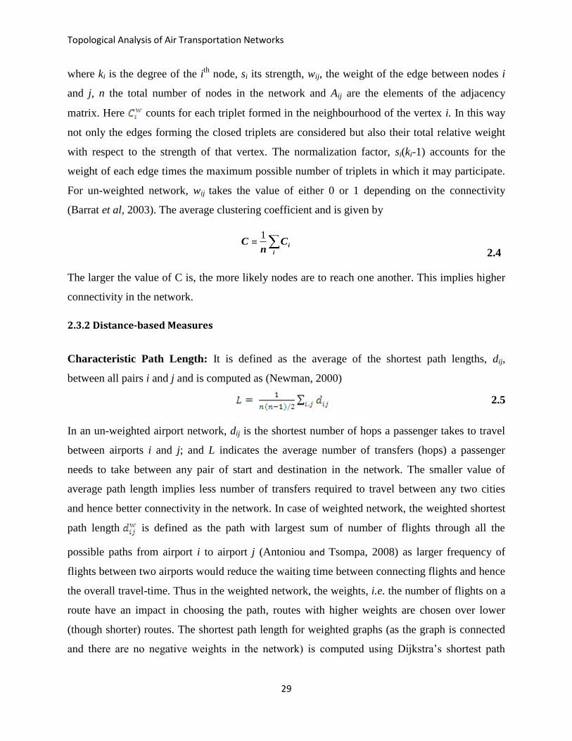
2.3.2 Distance-based Measures
Characteristic Path Length: It is defined as the average of the shortest path lengths, dij,
between all pairs i and j and is computed as (Newman, 2000)
2.5
In an un-weighted airport network, dij is the shortest number of hops a passenger takes to travel
between airports i and j; and L indicates the average number of transfers (hops) a passenger
needs to take between any pair of start and destination in the network. The smaller value of
average path length implies less number of transfers required to travel between any two cities
and hence better connectivity in the network. In case of weighted network, the weighted shortest
path length is defined as the path with largest sum of number of flights through all the
possible paths from airport i to airport j (Antoniou and Tsompa, 2008) as larger frequency of
flights between two airports would reduce the waiting time between connecting flights and hence
the overall travel-time. Thus in the weighted network, the weights, i.e. the number of flights on a
route have an impact in choosing the path, routes with higher weights are chosen over lower
(though shorter) routes. The shortest path length for weighted graphs (as the graph is connected
and there are no negative weights in the network) is computed using Dijkstra‟s shortest path

Topological Analysis of Air Transportation Networks
30
algorithm and is briefly described below (Dijkstra, 1959). In case of un-weighted network, on
putting weight = 1 on every flight-route, the Dijkstra‟s algorithm calculates minimum weighted
path by hop count.
Dijkstra’s algorithm:
For a given source node in the network, the algorithm finds the path with the lowest cost between
that node and every other node in the network. Here lowest cost corresponds to maximum weight
on edges; i.e. maximum no. of flights on the route. Let the source node be s. Initially set the
distance from node s to all other nodes in the network as infinity. Set distance zero for node s.
1. Mark all the nodes as unvisited. Set initial node as the current one.
2. For the current node, consider all its unvisited neighbors and calculate their tentative
distance (i.e. current node‟s distance from the previous iteration‟s current node + distance
of the node from current node). If this distance is less than the previously recorded
distance then replace it.
3. When all neighbors of the current node are considered, mark the current node as visited.
A visited node will not be checked again. The distance stored for the visited node is final
and minimal.
4. Set the new unvisited node with the smallest distance as “current” and repeat steps from
step no. 3.
5. If all nodes have been marked as visited, then stop.
For weighted network, using Dijkstra‟s algorithm, we calculated the shortest path length as the
path length which has maximum weight. Since in a transportation network, the shortest path
between nodes i and j will be the path having maximum number of flights between nodes i and j,
we normalize the weights such that the maximum weighted path is chosen:
= 1 – (wi,j/ (wmax + 1)) 2.6
(We choose wmax + 1 so as not to make the weight, wi,j, zero in case where wi,j = wmax otherwise it
would mean that there is not path.) The shortest path length for the weighted network is then
defined as
2.7
where is a path from vertex i to vertex j and is the set of all paths from x to y.
Topological Analysis of Air Transportation Networks
31
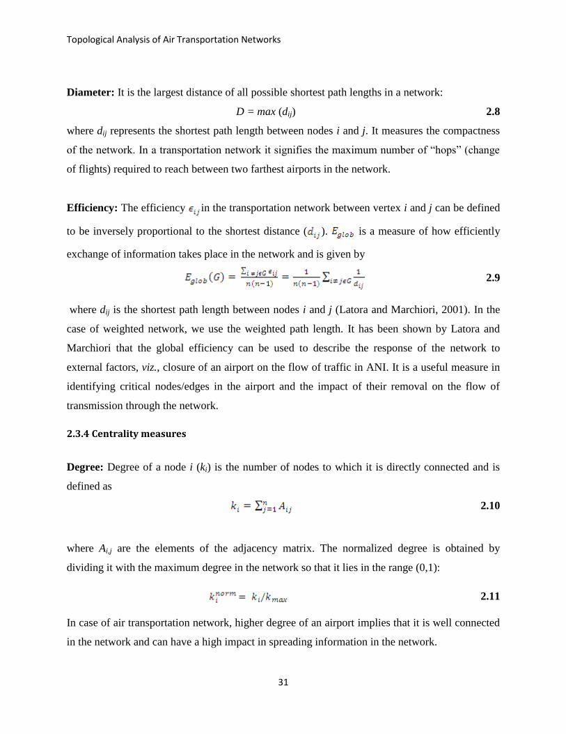
Diameter: It is the largest distance of all possible shortest path lengths in a network:
D = max (dij) 2.8
where dij represents the shortest path length between nodes i and j. It measures the compactness
of the network. In a transportation network it signifies the maximum number of “hops” (change
of flights) required to reach between two farthest airports in the network.
Efficiency: The efficiency in the transportation network between vertex i and j can be defined
to be inversely proportional to the shortest distance ( ). is a measure of how efficiently
exchange of information takes place in the network and is given by
2.9
where dij is the shortest path length between nodes i and j (Latora and Marchiori, 2001). In the
case of weighted network, we use the weighted path length. It has been shown by Latora and
Marchiori that the global efficiency can be used to describe the response of the network to
external factors, viz., closure of an airport on the flow of traffic in ANI. It is a useful measure in
identifying critical nodes/edges in the airport and the impact of their removal on the flow of
transmission through the network.
2.3.4 Centrality measures
Degree: Degree of a node i (ki) is the number of nodes to which it is directly connected and is
defined as
2.10
where Ai,j are the elements of the adjacency matrix. The normalized degree is obtained by
dividing it with the maximum degree in the network so that it lies in the range (0,1):
2.11
In case of air transportation network, higher degree of an airport implies that it is well connected
in the network and can have a high impact in spreading information in the network.

Topological Analysis of Air Transportation Networks
32
Betweenness: It is defined as the ratio of number of shortest paths passing through „i‟ to the total
number shortest paths in the network.
2.12
where Z(j-k) corresponds to all shortest paths from node j to node k and Z(j-k)(i) corresponds to the
shortest paths from node j to node k that pass from node i. Nodes having high betweenness
values are critical to the structural integrity of the network as most of the long range flights go
through them, and these nodes may represent a socioeconomic relevance for a specific region or
country itself. Thus in case of air transportation network, identifying such nodes is important as
inefficient functioning of these nodes can pose a risk of fragmenting network as these lie on the
multiple shortest paths. In case of modeling disease spread, identifying such nodes and cutting-
off/reducing flights through these nodes can help in delaying the spread of disease. The
normalized values of betweenness are obtained by dividing with the maximum betweenness
value in the network so that it lies in the range (0,1):
2.13
Closeness: It is defined as the reciprocal of the sum of shortest path between a node i and all
other nodes reachable from it:
2.14
where V is the connectivity component which contains all the vertices in the network reachable
from vertex i. Nodes having high closeness value will be more central in the network, i.e. all
other nodes can be reached easily from this node. Identifying such nodes can help in the planning
of efficient growth of the transportation network and in promoting tourism of not easily
reachable cities by increasing its closeness value. In case of modeling disease spread, identifying
such nodes and cutting-off flights to and from these nodes can also delay the spread of disease.
The normalized values of closeness are obtained by dividing with the maximum closeness value
in the network so that it lies in the range (0,1).
2.15

Topological Analysis of Air Transportation Networks
33
2.4 Results and Discussion
2.4.1. Analysis of ANI
2.4.1.1 ANI Exhibits Small-world Behavior
Many real world networks including social networks, WWW, gene networks, etc. have been
found to be small-world networks. Small-world networks are highly clustered like regular
lattices and yet have very small characteristic path length like random networks. The
mathematical formulation of the small-world behavior proposed by Watts and Strogatz is based
on the following two properties of the network: Characteristic path length, L and clustering
coefficient, C. For small-world networks, it has been observed that L ~ Lrand, C >> Crand. We
find that the clustering coefficient of undirected ANI is 0.626 and its characteristic path length is
2.23. To see if ANI exhibits small-world network properties, we randomize the connections in
ANI. The randomization for weighted and un-weighted ANI is achieved by following
mechanism.
a) For every edge, we randomly pick two vertices from 1 to 84.
b) We assign the weight on that edge to this new pair of vertices. In this way, by keeping the
total number of edges and nodes the same as that of ANI, we randomize the network such that
individual nodes do not preserve their degree or weights.
From Table 2.2, we see that the clustering coefficient of this randomized unweighted ANI is 0.14
while its characteristic path length is 2.53. Thus we observe that CANI >> Crand and LANI ~ Lrand,
suggesting small-world behavior of ANI. The smaller path length L of ANI suggests the presence
of long-range connections between otherwise very far (geo-spatially) and distant airports. For the
weighted ANI also we observe that CANI = 0.644 >> Crand = 0.166 and LANI =2.01 ~ Lrand = 2.57;
further confirming the small-world nature of ANI. For airport networks of China (weighted
ANC) and Brazil (BAN), the values of clustering coefficient and characteristic path length are
comparable, (CChina = 0.733, LChina = 2.067 and CBrazil = 0.64, LBrazil = 2.4) with that of weighted
ANI (C = 0.644, L = 2.15).

Topological Analysis of Air Transportation Networks
34
Table 2.2: The properties of different representations of weighted ANI are compared with
their randomized counterparts.
Property Undirected
Unweighted
Undirected
Weighted
Random
Unweighted
Random
Weighted
C 0.626 0.644 0.142 0.166
L 2.23 2.01 2.53 2.57
D 4 4 5 5
γ 2.19 2.238 -- --
k 3.04 3.04 3 3
P(>k) Power-Law Power-Law Poisson Poisson
We have analyzed weighted and un-weighted representations of undirected ANI. The properties
of these two representations with their randomized counterparts is summarized in Table 2.2. It
may be noted that the clustering coefficient of weighted ANI is slightly higher than that of un-
weighted ANI. Here, Cweighted > Cun-weighted means that weights on the edges forming the triplets
are large. So the high values of Cweighted reflects an efficient ANI in terms of both the structural as
well as the transmission properties, suggesting that most of the traffic-flow is occurring on the
routes that belong to interconnected triplets. In ANI, it is observed that the airports with higher
strength have connections with other airports having higher strengths indicating the “rich – club
phenomenon” (Barabasi and Albert 1999).
The most simplistic representation of ANI is an un-weighted, undirected network which
basically captures the connectivity information and it does not include information regarding the
number of flights on different routes, or the direction of flights. In Table 2.3 is summarized the
connectivity between 84 airports in India. There are 512 direct flight-routes between 84 airports
out of maximum possible number of flight routes, 7056, which is about ~ 7.25% of total flight-
routes, suggesting that ANI is a sparse graph. The low characteristic path length (~ 2) of ANI
implies that travel between majority of airport-pairs (67%) require one change of flight (Table
2.2). The diameter of ANI (D = 4) implies that travel between two farthest nodes in the network
would require 3 change-of-flights or hops. However, this number is very small, for 11 airport-
pairs out of a total of 7056. By introducing more direct-flight routes, the shortest path length and

Topological Analysis of Air Transportation Networks
35
diameter can be further reduced. It may be noted that India is a large country having 28 states
and 7 union territories in India.
Table 2.3: The percentage of flight routes falling on the shortest paths with the respective
hop count. Hop count gives the number of flights to be changed to reach the destination.
Shortest Path
length No. of Flight Routes Percentage Hop Count
1 512 7.25 0
2 4748 67.29 1
3 1785 25.29 2
4 11 0.15 3
However, we observe that only 226 pairs of state capitals and union territories out of a total of
1225 (35*35) pairs are directly connected to each other. It may be noted that missing links are
mainly from the airports in the eastern region, if all the state capitals are directly connected to
each other, it would increase the efficiency of the network, reducing the travel time and cost for
passengers and would also boost tourism especially in the eastern part of the country.
2.4.1.2 ANI Exhibits Scale Free Behaviour
Degree distribution: It gives us information about the spread or variation in the number of links
of the nodes in the network. In the random network, the links to any pair of nodes in the network
are added with fixed probability which is same for all vertices. Despite the random placements of
links the resulting system will have nodes having approximately the same number of links and
the degree distribution is given by Poisson distribution. Earlier all complex networks were
thought of having random network properties. However, Barabasi and Albert showed that most
real networks such as WWW or transportation network exhibit a power law behavior with a long
tail in their degree distribution (Barabasi and Albert, 1999). This indicates the presence of few
nodes, termed as “hubs”, having very large degree while majority of nodes have low degree.
Barabasi and Albert proposed preferential growth attachment as the mechanism for the evolution
of such networks; thus, nodes having high degree are more probable of getting new connections
than the ones with low degree resulting in power law behavior in their degree distribution. These
networks are termed as “scale-free” networks.

Topological Analysis of Air Transportation Networks
36
Figure 2.5: (a) The cumulative degree distribution for ANI shows power law behavior. (b)
The degree distribution on a log-log scale exhibits a straight line fit with exponent γcum =
1.19.
To analyze the distribution of flight routes handled by airports in ANI, we next analyzed the
distribution of the degree of nodes, P(k) in this network. Since ANI is a finite network (to reduce
fluctuations in the degree distribution), we consider cumulative degree distribution, P(>k) as a
function of degree, k, which defines the probability of a node having degree at least k. The
degree distribution can be approximated by the power law fit, given by the following
equation.
2.16
The scaling exponent, γcum , of the cumulative degree distribution P( >k) is related to that of
by γ = γcum +1 (Amaral et al, 2006). As shown in Fig. 2.5 (a), the cumulative degree
distribution follows a power law with exponent γcum = 1.19 (Fig. 2.5 (b)). Thus, the scaling
exponent of the degree distribution, P(k), is given by γ = γcum +1 = 2.29. This indicates the scale
free nature of ANI.
Strength and betweenness distribution: The degree of a node gives an idea about the
connection topology in the network. The identification of the most central nodes in the network
is the most important issue in network characterization. The most intuitive measure to find the
centrality would be the degree of a node; more connected nodes are more central. However the
degree alone does not provide complete information about the role of the node in the network;
because the highly connected network systems show lot of heterogeneity in the capacity and the
intensity of connections. To address this issue, we study the distributions of other centrality
Topological Analysis of Air Transportation Networks
37
measures: strength and betweenness. The connectivity between two airports is not only described
by the degree of the airports, but number of flights flying on a route and the traffic of flights at a
particular airport. For a better understanding of ANI, we need to consider the traffic managed at
particular airport as well. This is defined as the strength of the airport.
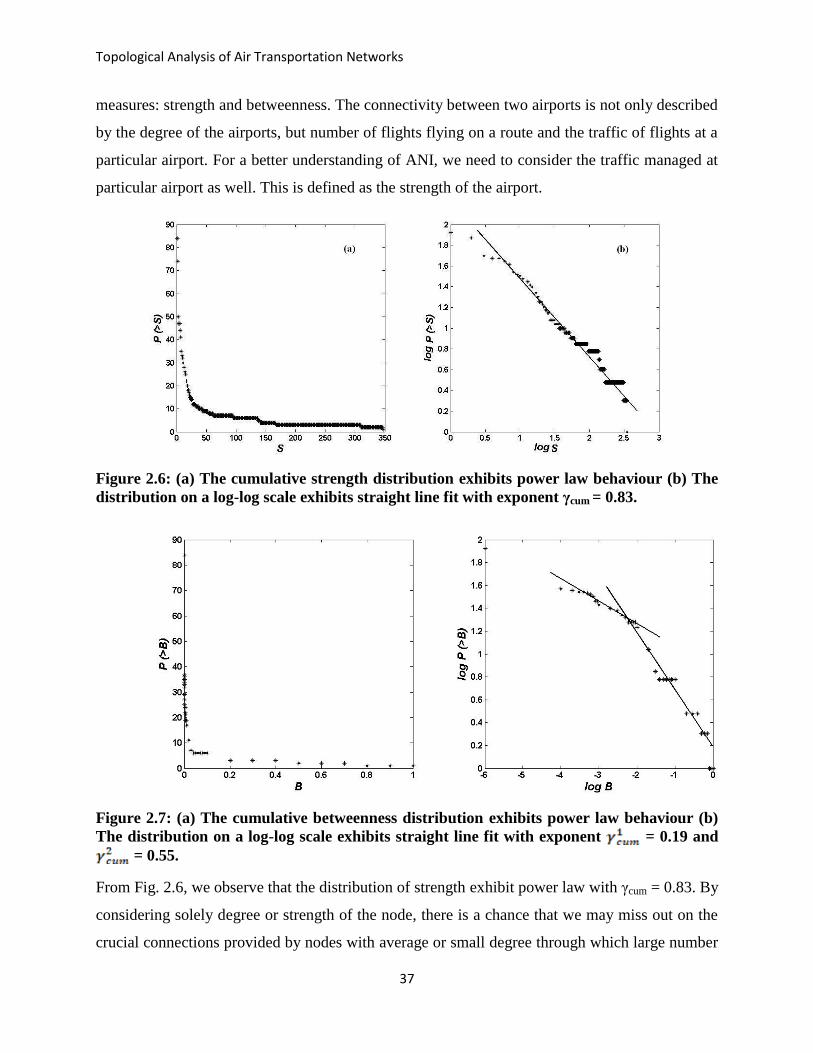
Figure 2.6: (a) The cumulative strength distribution exhibits power law behaviour (b) The
distribution on a log-log scale exhibits straight line fit with exponent γcum = 0.83.
Figure 2.7: (a) The cumulative betweenness distribution exhibits power law behaviour (b)
The distribution on a log-log scale exhibits straight line fit with exponent = 0.19 and
= 0.55.
From Fig. 2.6, we observe that the distribution of strength exhibit power law with γcum = 0.83. By
considering solely degree or strength of the node, there is a chance that we may miss out on the
crucial connections provided by nodes with average or small degree through which large number

Topological Analysis of Air Transportation Networks
38
of shortest paths pass. The presence of such bridges in the network is very important as the
absence of such bridges may tear apart the network into disconnected components during
accidental failures or targeted attacks. Such nodes are identified by the centrality measure
betweenness, B. The distribution of betweeness also exhibits double Pareto law as shown in Fig.
2.7 with the exponent values given by γ1
cum = 0.23 and γ2
cum = 0.55.
2.4.1.3 Assessing Risk and Efficiency of ANI
In the event of disease spread it would be most desirous to identify crucial airports and routes to
restrict transmission of disease in the whole country/region. However, complete close down of
traffic to and from important airports/routes is not economically viable. With this aim here we
have carried out an analysis of the effect of a percentage reduction in total flights from an
“important” airport on a particular route on the overall efficiency of the network. Most
importantly, it would be interesting to know (i) at what minimum percentage reduction of flights
the network would be robust with its connectivity intact, and (ii) at what percentage it would
completely collapse the network into its unconnected components. Such an analysis would not
only be useful in containing/delaying the spread of disease during an eventuality but also to
assess the loss of connectivity during closure of certain airports/routes in unavoidable weather
conditions, accidental failures, etc.
The response of scale-free networks to errors (random removal of nodes) and attacks (deliberate
removal of well connected nodes) have been well-studied. As shown above, ANI is a scale-free
network with small-world characteristics like high clustering coefficient and small characteristic
path length. The path length is usually defined for the connected graph. If certain nodes are
removed from the network, we may end up having disjoint clusters of the nodes. In such a case,
when there is no path between two vertices i and j, dij becomes infinite, making it impossible to
compute the average path length. To overcome this problem, Latora and Marchiori proposed a
measure termed as global efficiency. To define the global efficiency of graph G, assume that
every node sends information along the network through edges. The efficiency with which a
node i sends the information to the node j, is inversely proportional to the shortest distance
between i and j (Latora and Marchiori, 2001). Thus, when there exists no path between i and j,
and the shortest distance, dij, becomes infinite, efficiency is still defined, and equal to zero. Thus,
global efficiency, Eglob, enables the computation of the network‟s connectivity even when the

Topological Analysis of Air Transportation Networks
39
network has unconnected cluster of nodes. For ANI, Eglob = 0.47 (un-weighted) and Eglob = 0.55
(weighted). The efficiency of randomized ANI was found out to be 0.14 which is very low
compared to that of actual ANI. This suggests that ANI is quite an efficient network system. In
the next section, we show how these values are affected on random or targeted removal of nodes.
2.4.1.4 Analysis of Centrality Measures
The properties of scale-free networks have been extensively studied and these networks have
been shown to be robust against random removal of nodes but breaks down on targeted attacks.
Since ANI is shown to exhibit scale-free behavior, we expect that it may not be affected much by
accidental failures of airports but deliberate attack on important airports can cause the whole
network to collapse or have cascading effect of delay and cancellation of flights across the
network, a situation we typically observe during bad winter days resulting in cancellation of
flights from Delhi and the effect cascading to farther airports with large number of flights
delayed. For better organization of flights under such conditions, a good understanding of the
flow of transmission through the network is required. We this objective below we discuss the
effect of targeted removal of “important” nodes identified based on various centrality measures
such as degree, strength, betweenness and closeness and on the overall efficiency of the network.
In Table 2.4 is shown the comparison of top 10 airports listed based on these centrality measures.
We observe that top 6 cities are common for all the centrality measures viz. degree, betweenness
& closeness. This indicates that these 6 cities are not only the hubs in the network, but these lie
on the many shortest paths from other cities in ANI. Removal of any of the nodes may result into
disconnected clusters in ANI disturbing the connectivity. It is clear from the Table that Delhi and
Mumbai are the most important airports in the network, having not only highest number of
connections and total number of flights, but also in terms of their betweenness and closeness
values. Bengaluru has more number of flights (167) compared to Kolkata (141), however in
terms of betweenness, Kolkata is a more important airport as it is the „local‟ hub in the eastern
India and majority of flight-routes to the eastern cities go through Kolkata. Thus, in terms of
betweenness centrality, Delhi, Mumbai and Kolkata top the list, these being the local hubs in the
northern, western, and eastern region of India, respectively. However, since there are three local
hubs in the southern region, namely, Bengaluru, Hyderabad and Chennai, there is a drastic fall in
the betweenness value of these three airports. Goa, being most popular tourist destination, is well

Topological Analysis of Air Transportation Networks
40
connected to majority of local hubs and hence has higher closeness value compared to Guwahati
and Kochi; however in terms of strength and betweenness, it falls behind in the list as the airport
does not handle much traffic.
Table 2.4: Top 10 airports sorted based on their respective centrality values is listed. The
average values of degree (directed), strength, betweenness and closeness are 6, 25.06, 0.013
and 0.449 respectively.
Degree Strength Betweenness Closeness
Airport ki Airport Si Airport Bi Airport Cli
New Delhi 51 New Delhi 352 New Delhi 0.472 New Delhi 0.753
Mumbai 48 Mumbai 314 Mumbai 0.405 Mumbai 0.708
Kolkata 33 Bengaluru 167 Kolkata 0.229 Kolkata 0.629
Bengaluru 25 Kolkata 141 Bengaluru 0.138 Bengaluru 0.621
Hyderabad 23 Chennai 138 Chennai 0.112 Hyderabad 0.589
Chennai 21 Hyderabad 95 Hyderabad 0.083 Chennai 0.572
Ahmedabad 17 Ahmedabad 62 Guwahati 0.045 Ahmedabad 0.572
Goa 14 Guwahati 53 Kochi 0.037 Goa 0.556
Guwahati 13 Kochi 44 Ahmedabad 0.013 Guwahati 0.552
Kochi 11 Goa 37 Goa 0.009 Kochi 0.509
We observe from Table 2.4 that apart from degree, the other centrality measures also give us
insight about the interesting features of the network topology and evolution. So, it would be
interesting to investigate the effect of removing an airport based on various centrality measures
and analyze the efficiency of the network. This is discussed in detail below.
2.4.1.5 Analysis of Targeted Removal of High Degree Nodes
Here, we first discuss our analysis of impact on ANI when the high degree nodes are removed
from the network. This is done by computing the global efficiency of ANI, given in eqn. 2.8. In
Fig. 2.8 the global efficiency of un-weighted ANI is plotted as a function of random removal of
edges from the top six airports based on their centrality values. The edges are removed from
nodes randomly and efficiency is computed (The results are averaged over 10 random

Topological Analysis of Air Transportation Networks
41
configurations). Delhi being the capital and well connected to majority of the airports in the
country, reducing its connectivity, i.e. removing edges from Delhi has maximum effect on the
global efficiency of ANI, followed by Mumbai being the financial capital of the country, is also
well-connected. Thus, on gradually reducing the flight-routes from Delhi and Mumbai, a faster
fall in the efficiency of the network is observed, and on completely removing all the edges from
these two airports, the overall efficiency of the network falls by ~ 40.5%. However, no such
significant drop in efficiency is observed on removing any of the three local hubs in the southern
part of India, viz., Hyderabad, Chennai or Bengaluru, the traffic flow being well-distributed
among the three local hubs. The three southern hubs have direct flights to 9 common destinations
(~ 35%), both Bengaluru and Hyderabad and Bengaluru and Chennai share direct flights to 16
destinations (~ 65%), while Chennai and Hyderabad have 11 destinations in common (~ 45%).
Figure 2.8: Network efficiency is plotted as a function of reduction of edges (degree) from
six major hubs in an un-weighted ANI (Based on their degree): Delhi, Mumbai, Kolkata,
Bengaluru, Hyderabad, and Chennai and compared with that for random removal of
nodes (averaged over 10 random configurations). Efficiency falls rapidly after removal of
two major hubs Mumbai and Delhi.
Thus, though their degree values are high, their importance in the network is reduced beause of
the presence of two other local hubs in the southern region which provide alternate flight-routes.
Hence, cutting down edges from any one of these airports does not drastically affect the
efficiency of ANI, and even in the case of complete removal of either of these nodes, the
Topological Analysis of Air Transportation Networks
42
network efficiency drops only by about ~ 15%. However if we remove edges from all these three
southern hubs, then efficiency of the network reduces and the impact is simliar to that after
removing Mumbai or Delhi. This analysis suggests that developing more than one local hub
would not only ease the traffic flow but also develop healthy competition among airports
resulting in improved infrastructure, reduced fares, etc. as suggested by Malighetti et al (2009),
in their study on airport efficiency and centrality in the European network. Having more than one
local hubs can also provide alternate routes for diverting flights during emergencies such as bad
weather conditions and the network would not collape during targeted attacks or shutdowns of
airports. No significant effect on efficiency is observed on removing 20% of edges from any of
the randomly selected airports. This suggests that ANI is robust against random failures of
airports but vulnerable against targeted attacks.
2.4.1.6 Analysis of Weighted ANI
Since the traffic flow on various routes in ANI is not uniform, we next analyze a weighted
network where flights on edges are considered as weights. Typically, routes carrying heavy
traffic connect important airports; we analyze the impact of reduction of flights on the global
efficiency of ANI. It is clear from Table 2.4, that although Hyderabad and Bengaluru have
comparable degree (23 and 25 respectively), the strength of Bengaluru is much higher than that
of Hyderabad (167 and 95 respectively). The higher strength explains the political importance of
Bengaluru and also its emergence as India‟s Silicon Valley. Kochi, being the home for Southern
Naval Command, has more flights than Goa, which is a tourist spot, though Goa‟s degree is
higher. Thus it makes sense to take into consideration the strength (and not just connectivity) of a
node while analyzing its importance in the network. For example, in case of disease
transmission, an important question is how to restrict the spread of the disease through the
transportation network within the whole country or regions conducive of having larger impact
due to its climatic conditions. We would like to see if analysis of a weighted network can be
useful in this regard.
The complete close down of airport(s) with international connectivity is not a practical solution
as this would result in huge financial loss. Also, when we completely remove all the flights from
a particular pair of airports i.e. removal of an edge, it may cause a lot of inconvenience; e.g.
removing Delhi-Mumbai route, the path length increases from 2.15 to 2.63. An alternative

Topological Analysis of Air Transportation Networks
43
proposal would be to reduce a fraction of flights from the airport(s) on certain routes (i.e.
reducing the strength) but maintaining the connectivity. This is possible in a weighted ANI by
reducing a fraction of the weights on all the routes emanating from a high-centrality node and
computing the global efficiency to see its impact. (Here 100% removal of edges from a node is
equivalent to the removal of the node). The global efficiency for weighted ANI is found to be
0.55, which suggests that ANI is an efficient network system in terms of flow of information. In
Table 2.5 is shown the effect of reducing the strength of top six high-centrality nodes on the
efficiency of the network. We observe that unless we completely remove all the flights, the
reduction in efficiency of the network is not as significant as observed in the case of un-weighted
network (Fig. 2.8) because in this case the connectivity is still maintained. This behaviour in
depicted in Fig. 2.9. We see from Table 2.5 that when all the three southern hubs are removed,
the effect is similar to that observed in case of removal of Delhi (0.28) or Mumbai (0.32).
As in case of un-weighted ANI, the effect on efficiency is significantly higher in case of removal
of flights from Delhi and Mumbai. In the southern part of India, which contains three local hubs,
Hyderabad, Chennai and Bengaluru, no noticeable reduction in efficiency is observed even on
complete removal of the nodes. When flights from all the three southern local hubs are
completely removed, global efficiency value falls to 0.445.
Table 2.5: Effect of percentage reduction of flights from high strength nodes on the
efficiency of the overall network shown
%
Reduction
New
Delhi
(352)
Mumbai
(314)
Bengaluru
(167)
Kolkata
(141)
Chennai
(138)
Hyderabad
(95)
Hyderabad
+Chennai+
Bangalore
0 0.55 0.55 0.55 0.55 0.55 0.55 0.55
10 0.522 0.540 0.547 0.547 0.547 0.547 0.538
20 0.518 0.536 0.546 0.546 0.547 0.547 0.534
30 0.517 0.532 0.545 0.546 0.546 0.547 0.532
40 0.514 0.529 0.544 0.545 0.546 0.546 0.529
50 0.510 0.527 0.544 0.545 0.545 0.546 0.522
60 0.507 0.525 0.543 0.544 0.545 0.546 0.516
70 0.505 0.523 0.542 0.544 0.545 0.546 0.514
80 0.503 0.521 0.542 0.544 0.544 0.545 0.510
90 0.501 0.520 0.542 0.543 0.544 0.545 0.503
100 0.401 0.407 0.519 0.509 0.522 0.524 0.432

Topological Analysis of Air Transportation Networks
44
Figure 2.9: The effect on global efficiency after percentage reduction of flights from 6
important hubs based on their strength in ANI.
Even when 90% of flights are cut off the efficiency of the network is still very good. Since the
spread of infectious disease is directly proportional to the number of passengers traveling which
in turn will depend on the number of flights operating. While removing flights we are still
maintaining the connectivity and robustness of the network intact and network would not
collapse. We are only limiting the flux of passengers moving across the cities through air
transport. Thus, limiting the number of flights would result in the delay of spread of the
infectious disease.
2.4.1.7 Analysis of Removal of High-Betweenness Nodes
Betweenness is a parameter that enumerates the importance of a node in terms of it being central
to the traffic-routes in the network. Most high-degree nodes have been observed to be having
high values of Betweenness also, e.g., Mumbai and Delhi, and further confirm the importance of
these airports to the entire traffic dynamics. The airports in the most remote northern or eastern
places of India, viz., Jammu, Shillong, etc., have betweenness values close to zero as these

Topological Analysis of Air Transportation Networks
45
airports do not fall on any shortest paths and removal of these nodes do not have any appreciable
effect on the whole transportation system. It is observed that out of 84 airports, 37 airports have
betweeenness value as zero, i.e. no shortest path goes through these airports. Some of these are
the state capitals such as Shillong (Meghalaya). Also capitals like Port Blair (B= 0.0001,
Andaman and Nicobar), Itanagar (B = 0.0001, Arunachal Pradesh), Dispur (B = 0.00, Assam),
Daman, Gandhinagar (B = 0.0002, Gujarat), Shimla (B = 0.00, Himachal Pradesh), Gangtok (B =
0.00, Sikkim) either do not have a functional airport or their betweenness values are very low.
That is, airports with poor accessibility have low betweenness value, and if these cities are tourist
spots or state capitals, there exists a need to increase more flights through these airports to
improve tourism, e.g. Kullu-Manali, Jammu, etc. On the other hand, if a high-betweenness node
such as Kolkata is removed, accessibility to majority of the eastern cities is completely cut-off
from the rest of the country, while for some other cities, the “hops” or change of flights, to reach
their destination increases. In Table 2.6 is summarized the effect of cutting off flights from Delhi
to top six ranking betweeness airports. For example, on removing flights on the route Delhi to
Kolkata, out of 8 airports in eastern India, hop-count increases for 6 of them to reach Delhi.
Similarly, on removing the Delhi-Mumbai route, five airports in the western part of India are
affected. This can have important implications in the spread of an infection through air-
transportation network; by restricting flights on certain routes, delay in the spread of disease to
various regions can be achieved, if so desired. However, no such pattern is observed in the case
of removing flights from Delhi to either Hyderabad, Chennai, or Bengaluru, probably because of
their close proximity in the southern region and as they share over 50 % of destinations among
themselves. If, similarly, local hubs are developed in the eastern region, for example, it would
help in the economic development of the region. It should also be noted that when we improve
efficiency of the network, it helps in better connectivity, faster economic growth of the region,
higher revenue generation; however, it may have adverse effects in case of spread of infectious
disease, or malfunctioning of airport due to bad weather. Thus centrality measure analysis is
useful in undertaking preventive measures in the two contrasting scenarios. Thus we see how the
analysis of betweenness centrality of an airport can be useful in guiding the direction for the
growth of the network by identifying the important airports/routes. On removal of top 6 high
betweenness nodes, the network is divided into 4 sub clusters and 9 lone nodes; which are
basically the disconnected components of the network.

Topological Analysis of Air Transportation Networks
46
We introduced links to the state capitals which are not connected to each other, to improve their
centrality values, and to analyze the impact on network efficiency. We observed that when we
added just one more edge to 28 state capitals, and connected them to one of the other capitals
(randomly and if not previously connected) then we observed that average betweenness value of
the network increased to 0.02 from 0.013; and the efficiency of the network increased to 0.521
from 0.47.
Table 2.6: The increased “hops” for certain smaller airports when flights from Delhi to six
high-betweenness airports are cut-off is summarized.
Mumbai Solapur (3) Nasik (3) Bhava-nagar
(3)
Kandla
(3) Rajkot (3)
Kolkata Aizwal (3) Dimapur
(3) Shillong (3) Jorhat
(3)
Lilabari
(3)
Gaya
(3)
Silchar
(3)
Tezpur
(3)
Bengaluru Agatti (3) Madurai
(3)
Mangalore
(3)
Chennai Tiruchirapalli
(3)
Hyderabad Vijaywada (3) Hubli (3)
Guwahati Lilabari (3)
2.4.1.8 Analysis of High Closeness Nodes
The closeness centrality is a measure of the accessibility of an airport to any other airport in the
country. For ANI, we observe that 37 out of 84 airports have closeness value greater than
average closeness value (~ 0.45), suggesting a good inter-connectivity between cities. Here we
show that the analysis of this measure can have important implication in developing tourism to
hill stations (e.g., Kullu Manali, Darjeeling, Mount Abu, Gir Jungle Resort, etc.), wild-life
sanctuaries (e.g., Corbett National Park, Sundarban National Park, etc.), historical places (e.g.,
Agra, Hampi, Khajuraho, etc.) and religious places (e.g., Puri, Tirupati, Amritsar, etc.) apart
from improving connectivity to major industrial cities (e.g., Jamshedpur, Ankleshwar, etc.). Goa,
being the popular tourist sport in India, is connected to most of the hubs in the networks, viz.
Delhi, Mumbai, Kolkata, Bangalore etc. and hence removing flights from any one of the hubs
does not affect its closeness value much.
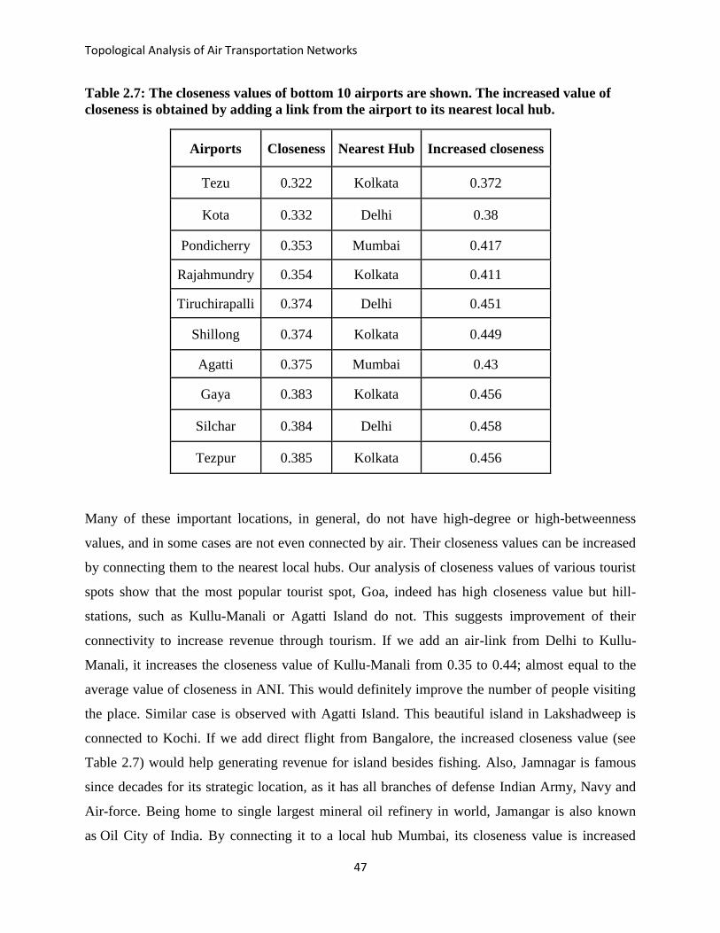
Topological Analysis of Air Transportation Networks
47
Table 2.7: The closeness values of bottom 10 airports are shown. The increased value of
closeness is obtained by adding a link from the airport to its nearest local hub.
Airports Closeness Nearest Hub Increased closeness
Tezu 0.322 Kolkata 0.372
Kota 0.332 Delhi 0.38
Pondicherry 0.353 Mumbai 0.417
Rajahmundry 0.354 Kolkata 0.411
Tiruchirapalli 0.374 Delhi 0.451
Shillong 0.374 Kolkata 0.449
Agatti 0.375 Mumbai 0.43
Gaya 0.383 Kolkata 0.456
Silchar 0.384 Delhi 0.458
Tezpur 0.385 Kolkata 0.456
Many of these important locations, in general, do not have high-degree or high-betweenness
values, and in some cases are not even connected by air. Their closeness values can be increased
by connecting them to the nearest local hubs. Our analysis of closeness values of various tourist
spots show that the most popular tourist spot, Goa, indeed has high closeness value but hill-
stations, such as Kullu-Manali or Agatti Island do not. This suggests improvement of their
connectivity to increase revenue through tourism. If we add an air-link from Delhi to Kullu-
Manali, it increases the closeness value of Kullu-Manali from 0.35 to 0.44; almost equal to the
average value of closeness in ANI. This would definitely improve the number of people visiting
the place. Similar case is observed with Agatti Island. This beautiful island in Lakshadweep is
connected to Kochi. If we add direct flight from Bangalore, the increased closeness value (see
Table 2.7) would help generating revenue for island besides fishing. Also, Jamnagar is famous
since decades for its strategic location, as it has all branches of defense Indian Army, Navy and
Air-force. Being home to single largest mineral oil refinery in world, Jamangar is also known
as Oil City of India. By connecting it to a local hub Mumbai, its closeness value is increased
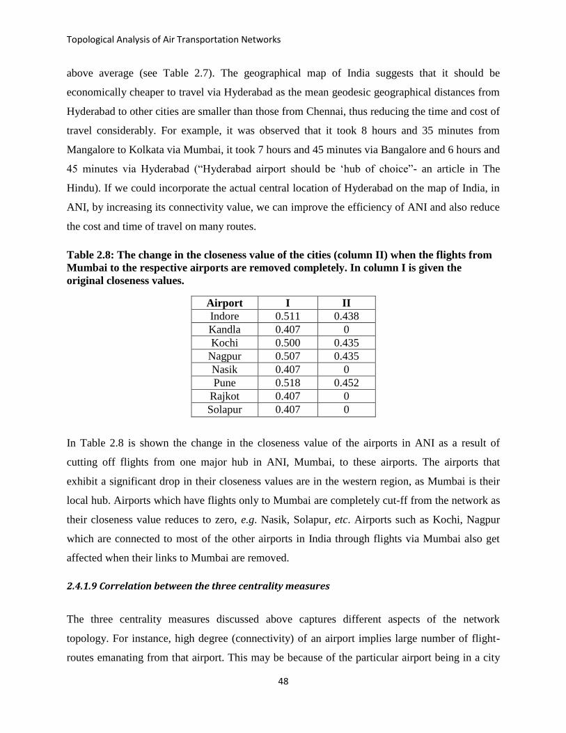
Topological Analysis of Air Transportation Networks
48
above average (see Table 2.7). The geographical map of India suggests that it should be
economically cheaper to travel via Hyderabad as the mean geodesic geographical distances from
Hyderabad to other cities are smaller than those from Chennai, thus reducing the time and cost of
travel considerably. For example, it was observed that it took 8 hours and 35 minutes from
Mangalore to Kolkata via Mumbai, it took 7 hours and 45 minutes via Bangalore and 6 hours and
45 minutes via Hyderabad (“Hyderabad airport should be „hub of choice”- an article in The
Hindu). If we could incorporate the actual central location of Hyderabad on the map of India, in
ANI, by increasing its connectivity value, we can improve the efficiency of ANI and also reduce
the cost and time of travel on many routes.
Table 2.8: The change in the closeness value of the cities (column II) when the flights from
Mumbai to the respective airports are removed completely. In column I is given the
original closeness values.
Airport I II
Indore 0.511 0.438
Kandla 0.407 0
Kochi 0.500 0.435
Nagpur 0.507 0.435
Nasik 0.407 0
Pune 0.518 0.452
Rajkot 0.407 0
Solapur 0.407 0
In Table 2.8 is shown the change in the closeness value of the airports in ANI as a result of
cutting off flights from one major hub in ANI, Mumbai, to these airports. The airports that
exhibit a significant drop in their closeness values are in the western region, as Mumbai is their
local hub. Airports which have flights only to Mumbai are completely cut-ff from the network as
their closeness value reduces to zero, e.g. Nasik, Solapur, etc. Airports such as Kochi, Nagpur
which are connected to most of the other airports in India through flights via Mumbai also get
affected when their links to Mumbai are removed.
2.4.1.9 Correlation between the three centrality measures
The three centrality measures discussed above captures different aspects of the network
topology. For instance, high degree (connectivity) of an airport implies large number of flight-
routes emanating from that airport. This may be because of the particular airport being in a city

Topological Analysis of Air Transportation Networks
49
that is either politically or financially important (e.g., Delhi and Mumbai) and hence is well-
connected with other cities of the country. The betweenness measure identifies importance of an
airport based on how many shortest paths connecting any two airports pass through it. If that
airport gets closed, it would result in increasing the shortest path length for many pairs of
airports. Thus, removal of high betweenness nodes would result in an increase in the hop count,
i.e., change of flights required, partitioning the network into separate modules. Closeness values
highlight the importance of an airport in terms of its accessibility from other airports, higher the
closeness centrality of a node, higher is its accessibility.
Figure 2.10: Correlations between (a) betweenness and closeness (b) degree and closeness,
and (c) degree and betweenness, are shown.
Next we analyzed pair-wise correlations between the centrality measures, viz., Degree,
Betweenness and Closeness. In Fig. 2.10 is shown the correlation between the three centrality
measures, taken pair-wise. The correlation between betweenness and closeness (r = 0.62) or
between degree and closeness (r = 0.54) shown in Fig. 2.10 (a) and (b) respectively, suggest that
nodes having high closeness value need not have high values of degree or betweenness. In Fig.
2.8(c) is seen that correlation between degree and betweenness is very high (r = 0.95) suggesting
that nodes having high degree also have high betweenness values in ANI, though there are a few
exceptions. Hence for identifying a crucial node one may consider either degree or betweenness

Topological Analysis of Air Transportation Networks
50
measure, however, degree is much easier to compute than Betweenness as degree is just the sum
of the connections a node has while for betweeness we have to calculate the shortest paths
passing through every node.
2.4.2 Analysis of WAN
In this section, we extend our study to a larger transportation network the world airport network
(WAN) as shown in Fig. 2.3 (b), of which ANI is a subpart. The importance of the analysis
WAN goes beyond the convenience it provides to the world travelers. The exhaustive analysis of
WAN has been previously done by many others, including the pioneering work by Guimera and
Amaral (2005). Since the airline traffic across the world has now tremendously increased, it is
important to understand and take measures for any disturbances developed due to climatic
changes, emergencies such as terror attacks, crisis etc. as these get easily propagated through the
densely connected airport network and have cascading effect to farther regions. Here we present
our analysis of some topological properties of WAN to understand the network stability in
undesirable conditions such as percolation of delays due to climatic conditions and spread of
infectious diseases.
2.4.2.1 WAN as Small World and Scale Free Network
The average shortest path length of WAN is the average minimum number of flights one needs
to take to reach any city from any other city across the globe. The clustering coefficient C, gives
the idea about transitivity in the network and is defined as the probability that two cities that are
directly connected to a third city are also directly connected to each other. We observe that WAN
exhibits high clustering coefficient, C = 0.611 and small average path length, L = 4.27 (un-
weighted), in agreement with those reported by Guimera and Amaral (2005) in their earlier
study: C = 0.62 and L = 4.4. Similar to ANI, the world airport network was randomized keeping
the total number of nodes and connections fixed as in actual WAN. For this randomized WAN,
the clustering coefficient, C = 0.059, is much lower while the path length L = 5.183, is similar to
that of actual WAN, indicating that WAN is a small world network (Watts and Strogatz, 1998).
To understand the evolution and structure of WAN, we next analyzed the degree distribution of

Topological Analysis of Air Transportation Networks
51
WAN. The cumulative degree distribution is shown in Fig 2.12. It tells us about the number of
airports having degree greater than k and from Fig. 2.12. (a), we observe that for WAN, degree
distribution follows a power law.
Figure 2.12: The degree distribution of world airport network plotted on (a) normal scale
and on (b) log-log scale with the scaling coefficient γcum = 1.08.
We also find that the betweenness distribution of WAN follows power law from Fig. 2.13 (a) and
(b) suggesting that very few nodes in WAN have a very high betweenness values. (γcum = 1.08
from Fig. 2.12 (b)). Gumeral and Amaral found out the exponent value γcum = 1.0.
Fig. 2.13 The betweenness distribution of the world-wide air transportation network is
plotted on (a) normal scale. It gives a power law distribution (b) when log-log values are
plotted with γcum = 1.24 on linear scale.

Topological Analysis of Air Transportation Networks
52
2.4.2.2 Centrality Measure Analysis
The degree of the node tells us about its connectivity of the node in the network. It is also one of
the important centrality measures which is very easy to calculate. Since WAN is a scale free
network it has a few nodes with large connectivity, called “hubs” and majority of nodes have a
low degree. It is observed that some nodes with low degree play an important role in maintaining
the stability of the network. An airport may not be connected to large number of other airports,
but a very large number of shortest paths may pass through it. This information is quantified by
the centrality measure, betweenness. It would be worth identifying nodes having high
betweenness as these nodes may be critical in spreading delays/infections through the network.
Similarly closeness gives us an idea about the importance of the node in terms of its accessibility
from other nodes in the network. Such nodes would improve the connectivity of the network by
reducing the diameter/path length of the network. For a node to have large closeness value, it
need not be well connected or lie on a large number of shortest paths. If it is connected to a hub,
its closeness value increases as it then becomes only one hop away from all the airports that hub
is connected to. Thus the efficiency of the network can be improved by increasing closeness
values of the small airports. Hence, these centrality measures, betweenness and closeness, are
very important to understand the structure and topology of the complex networks.
Anomalous Centrality Behavior in WAN
Betweenness is defined as the ratio of number of shortest paths passing through „i‟ to the total
number shortest paths in the network. Nodes having high betweenness values are critical to the
structural integrity of the network. Previously, Guimera and Amaral showed that in WAN, the
most connected nodes are not necessarily the nodes with high betweenness values i.e. the
shortest paths need not pass only through the nodes with high degree. Nodes having small degree
can have high betweenness values if they are central to two communities of nodes. Here we
show such anomalies for the nodes with small degree and large betweenness centrality values,
the airports that connect two or more continents in WAN. For ANI we did not observe such an
anomaly as we found that most high-betweenness nodes were the ones with high degree. In table
2.9 we list the top 25 airports according to their betweenness value along with their degree. From
Table 2.9, it can be seen that Anchorage, Sao Paulo, Brisbane and Johannesburg have very low

Topological Analysis of Air Transportation Networks
53
degrees compared to the top 5 high degree airports; however their betweenness values are
comparable to that of Frankfurt, Paris etc.
Table 2.9: The airports with their IATA code are arranged according to their betweenness
values (Top 25). The highlighted airports show anomaly with small degree yet higher
betweenness values. Starred (*) airports do not fall in the list of top 25 high degree nodes.
Airport Code City Betweeness b Degree k
FRA Frankfurt 0.0890 266
ANC* Anchorage 0.0737 50
LAX Los Angeles 0.0678 230
CDG Paris 0.0666 251
LHR London 0.0546 247
GRU* Sao Paulo 0.0541 93
PEK Beijing 0.0520 175
ORD Chicago 0.0491 280
ATL Atlanta 0.0431 178
YYZ Toronto 0.0427 158
SIN Singapore 0.0412 151
AMS Amsterdam 0.0401 189
DXB* Dubai 0.0390 149
JFK New York 0.0389 174
NRT* Tokyo 0.0382 122
BNE* Brisbane 0.0341 68
SYD* Sydney 0.0339 109
ICN Seoul 0.0327 150
SEA* Seattle 0.0326 109
BKK* Bangkok 0.0324 146
DME* Moscow - 0.0311 121
DEN Denver 0.0309 231
JNB* Johannesburg 0.0284 90
AKL* Houston 0.0278 68
YUL* Madrid 0.0271 89
The reasons for such high betweeness values for these low degree airports are their geographical
locations, and political importance. Consider an example of Johannesburg (JNB). The city is
without doubt South Africa's financial hub and Johannesburg Airport (JNB) is therefore of great
commercial importance to business travelers. Johannesburg is home to a major African stock
exchange and is a notable connection point for tourists heading to Cape Town, Durban and for a
safari holiday at the highly acclaimed Kruger National Park. It is well connected to many

Topological Analysis of Air Transportation Networks
54
countries in various continents such as Europe and America. The other airports in the southern
part of Africa are not so well connected to the world airports with direct flights but these are
connected only through Johannesburg.
Although Johannesburg does not have large number of connections, it does have important
connections to cities in Europe such as London, Paris, etc. and hence acts as the central airport
joining two communities; Africa and rest of the world. This explains the higher betweenness
centrality value of Johannesburg. Similar explanation can be given for the high betweenness and
low degree of Sao-Paulo International airport (GRU) in Brazil, which is an important airport in
South America. Being the important airport in Latin America, it has the maximum traffic
movement as most of the Latin American airports are connected to it. Although this airport was
put in the world's third place in number of delayed flights, it is connected to most of the
important hubs in WAN and would be responsible for delay cascading to other airports in the
world. The nodes with high betweenness and low degree play an important role in diffusion and
congestion and in the cohesiveness of the complex networks. Guimera and Amaral (Guimera and
Amaral, 2005) suggested that the origin of such anomalous behavior points can be useful in
finding communities in the network. The importance of such airports in the network cannot be
neglected due to the following main reasons: (1) these airports mainly connect two communities
in the network which otherwise would result into disconnected clusters. (2) These airports play
key role in maintaining traffic flow and cohesiveness of the network.
We observed a similar anomalous behavior in the closeness centrality as seen in Table 2.10. We
see that Zurich, which is the capital of Switzerland and the most famous tourist spot in the world,
has degree almost half that of Frankfurt (which has the 2nd
highest degree in the world from
Table 2.12); however their closeness values are comparable. Zurich is connected to most of high
degree and high betweenness nodes in the world, mostly the capitals of the countries from
different continents. Similar is the case for Palma de Mallorca airport. The boom in tourism
caused Palma to grow significantly, with visiting passengers increasing from 5,00,000 in 1960 to
192,00,000 in 2001 (per year). Although degree of Palma de Mallorca is significantly lower than
that of Paris or Frankfurt, it is connected to all the major cities in Europe as well as United states,
resulting in higher closeness value which is beneficial for tourism purpose.

Topological Analysis of Air Transportation Networks
55
Table 2.10: Anomalies in degree and closeness values of the airports in WAN. The average
closeness value for WAN= 0.247.
Airport City Closeness Degree
FRA Frankfurt 0.4052 266
CDG Paris 0.3944 251
AMS Amsterdam 0.3900 189
LHR London 0.3886 247
JFK New York 0.3848 174
LAX Los Angeles 0.3798 230
YYZ Toronto 0.3790 158
DXB Dubai 0.3783 149
ATL Atlanta 0.3777 178
AMM Amman 0.3712 65
ZRH Zurich 0.3712 137
DOH Doha 0.3623 76
SFO San Francisco 0.3619 161
BKK Bangkok 0.3615 146
IAH Houston 0.3611 170
MRU Plaisance 0.3611 26
CUN Cancun 0.3611 66
JAX Jacksonville 0.3512 31
HKG Hongkong 0.324 145
PMI Palma de Mallorca 0.3128 124
Similarly, Mauritius, a nation with just 2040 square km. of area has attracted a wide attraction
from tourists all over the world. The links connected to Plaisance airport in Mauritius are just 26,
almost one tenth of the highest degree of the airport in WAN, however its closeness value is very
high. It is connected to most of the high degree nodes in the network with direct flights, which
improved its closeness value. From this analysis we can propose that to increase tourism, or
increase accessibility to large number of airports, it is not necessary to increase its connectivity;
just by connecting it to few major airports in different continents and sub-continents would
suffice.
Effect of Closing down of Major Hubs in WAN during Volcanic Ash Activity: A Case
Study

Topological Analysis of Air Transportation Networks
56
As discussed above in the analysis of an ANI, compared to the connectivity (degree) of a node,
strength is a more useful measure as it also incorporates the traffic flow through the airport, for
e.g., two airports having same degree but operating different number of flights do not have the
same impact on the flow of traffic through the network. Sudden system failures or adverse
weather conditions can affect the strength of the airports as a consequence of flight cancellations
and in the extreme case may even result in connectivity collapse of the network.
Table 2.11: Traffic at main airports of Europe, April, 2010.
Airport Departures/day
(April, 2010)
Change since
April, 2009(%)
Paris 599.9 -20%
Madrid 588.9 -4%
Frankfurt 538.1 -16%
London 526.2 -20%
Amsterdam 457.4 -20%
Muenchen 454.4 -18%
Rome 434.9 -5%
Barcelona 370.3 -8%
Istanbul 358.6 -3%
Vienna 329.7 -6%
Zurich 297.9 -13%
Copenhagen 272.3 -15%
Athinai 269.5 -6%
Brussels 253.4 -21%
Oslo 248.6 -12%
Duesseldorf 238.0 -17%
Milano 237.3 -11%
Palma 216.4 -8%
Here, we discuss the example of the eruption of Eyjafjallajoekull glacier in Iceland in April 2010
which led to major disruptions in the air travel, not only in northern Europe, but the effect was
felt across the whole world with a number of flight cancellations and many more delayed,
leaving airline passengers stranded around the globe. More than 95,000 flights were cancelled
across Europe during the six days of disruption with about 20 countries closing down their
airspace and affecting hundreds of thousands of travelers. Global airlines lost about $1.7bn of

Topological Analysis of Air Transportation Networks
57
revenue as a result of the disruptions caused by the Icelandic volcanic eruption. In April 2010,
the average delay per delayed flight for departure traffic from all causes of delay was reported to
be 27.2 minutes, an increase of 11% on the same month last year
(http://www.eurocontrol.int/coda/). Airlines rely on a carefully-planned sequence of flights.
Once the sequence is broken, it is very hard to catch up, particularly on complex routes such as
the UK to Asia or Australia.
Table 2.12: Top 10 airports with high centrality measures in WAN
City Degree City Betweenness City Closeness
Chicago 280 Frankfurt 0.089 Frankfurt 0.405
Frankfurt 266 Anchorage 0.073 Paris 0.394
Paris 251 Los Angeles 0.067 Amsterdam 0.390
London 247 Paris 0.066 London 0.388
Denver 231 London 0.054 New York 0.384
Los Angeles 230 Sao Paulo 0.054 Los Angeles 0.379
Madrid 193 Beijing 0.052 Toronto 0.378
Amsterdam 189 Chicago 0.049 Dubai 0.378
Munich 181 Atlanta 0.043 Atlanta 0.377
Atlanta 178 Toronto 0.042 Newark 0.374
As WAN is observed to be a scale free network, though it is robust against random attacks, it is
vulnerable and may collapse if the hubs are affected. The volcanic ash activity forced most of the
European hubs, e.g. Frankfurt, London, etc. to close down completely and hence the
transportation network was severely affected. When focusing on the top 20 airports by daily
departures, all of the top 20 saw reductions in their average daily flights due to the disruption
caused by the volcanic ash. There were around 11% of fewer flights in April 2010 flying from
and to Europe. These cancellations of flights required the need of finding alternative flight
routes. The main challenge in this case was to find the second best and not so affected airports so
that traffic flow could be diverted to such airports. This requires an analysis of the topological
properties of WAN. From Table 2.11, we see that Barcelona was one of the airports which was
affected a bit less by the ash cloud. Most of the Swedish and Norwegian tourists in Egypt or
Mallorca or Canary Islands were hence flown back to Barcelona and then were taken back home
by road. This kind of en routing caused a large amount of delay and inconvenience for the
passengers. The degree value of Barcelona is very high, 171, indicating a large number of

Topological Analysis of Air Transportation Networks
58
connections. However, it ranks 171th
in the list of betweenness value and even lower in terms of
its closeness value. If the centrality measures of such airports are improved by improving its
connections to other parts of the world apart from Europe, then it would have helped in this
situation. Most of the airports in southern Europe were seen to be affected less, but there are very
few international flights from these airports. If certain hubs are developed in this region then it
would help in providing alternative routes in such situations. As it can be seen from Table 2.11,
there were notable changes at the major European hubs of Paris (CDG), Frankfurt (FRA),
London (LHR) and Amsterdam (AMS). These airports are not only the major hubs in Europe but
in the world, and also act as the central points to connect cities from Asia, Africa and America.
From Table 2.12, it can be seen that these are also the top four airports by their closeness values.
Due to the shutting down of these airports, a cascading effect was observed at other airports too,
causing delays at the world‟s top hubs. As most of these four airports have large number of
flights to and from New York, as a result about 50% of the departures in New York were
affected.
2.4.2.3 Global Efficiency of WAN
WAN is a small world network with small path length of L = 4.27 suggesting that any two
airports can be reached by changing 4 flights in between. However if certain airports stop
functioning due to bad weather or are closed down as precautionary measures to contain the
spread of disease, then the network may result into the disconnected clusters. In this case, path
length L would not give us the correct idea about network connectivity, hence as before in the
case of ANI, we compute global efficiency, Eglob, (Latora and Marchiori, 2001). The global
efficiency of un-weighted WAN was found out to be 0.62 which indicates that WAN is an
efficient network system. To understand the effect of removal of nodes on global efficiency, we
next analyzed removal of connections (partially/fully) from nodes with high centrality values.
Unlike ANI, we find that removing edges from one or two top nodes does not affect the
efficiency much as shown in Table 2.13. But when we removed connections from top 10 high
centrality nodes, significant effect on efficiency was observed. We observe that on 100%
removal of edges, (i.e. corresponding to removal of the nodes), the efficiency drops to almost
two-third of the original efficiency when the nodes are removed based on their betweenness
value. Also the effect was not the same when we removed edges from nodes with high degree,

Topological Analysis of Air Transportation Networks
59
high betweenness and high closeness. The reason lies in the anomaly which was described
before. The edges from nodes are removed randomly and we have taken the average over 10
calculations. When we remove all the edges from a node, then it is equivalent to the removal of
the node itself, from the network. We see that 6 nodes from the list of top 10 airports with high
degree values are European airports (Table 2.12). During the volcanic ash eruption in 2010, all of
these six airports were completely closed down. If we remove all connections from just these six
airports in WAN, the efficiency of WAN falls down to 0.493.
Table 2.13: Efficiency of the network shown on % reduction of edges from top 10 centrality
nodes, viz. Degree, Betweenness and Closeness. Note that 100% removals of edges
correspond to removal of the node itself.
% Reduction
of edges
Degree Betweenness Closeness
10 0.606 0.604 0.614
20 0.601 0.602 0.611
30 0.597 0.593 0.602
40 0.588 0.584 0.595
50 0.581 0.578 0.590
60 0.576 0.569 0.585
70 0.572 0.558 0.579
80 0.565 0.551 0.571
90 0.561 0.543 0.566
100 0.442 0.417 0.455
These airports have flights from Asia, Africa and America and they are connected to most of the
countries in these three continents with direct flights. Closing down of these airports therefore
had severe effects on the robustness of the network and the connectivity collapsed badly during
that period. We find that removal of top nodes based on their betweenness value has the greater
impact on the efficiency of the overall network (Fig. 2.14). The nodes with more connections are
not necessarily the central nodes in WAN. After removing all the connections from a node with
high betweenness value, the different communities in the network may get disconnected as the
particular node may be acting as a bridge connecting the two communities.

Topological Analysis of Air Transportation Networks
60
Figure 2.14: Effect on global efficiency when edges from top 10 nodes are removed based
on the centrality value of nodes.
2.4.2.4 Correlation between the centrality measures
It is seen from Fig 2.14 that the effect on global efficiency after removing edges from the nodes
chosen according to their degree and closeness is almost similar, indicating that both the
measures almost give the same set of nodes. Although the correlation coefficient for the three
pairs of the three centrality measures are very low (rbet-deg = 0.02, rdeg-clos = 0.11, rclos-bet = 0.07)
for the complete WAN, we find for top 5% of the nodes in WAN, the correlation between degree
and closeness (rdeg-clos = 0.62) is high compared to that of betweenness measure with degree or
closeness (rbet-deg = 0.03 and rclos-bet = 0.06). Generally airports with very high degree are
connected to other most connected airports and this helps in increasing their closeness values.

Topological Analysis of Air Transportation Networks
61
CHAPTER 3
Modeling of Air Transportation Network
3.1 Introduction
Graph theory or network science has been applied to various practical problems since long time
and has its roots as far back as 18th
century. A network can be defined by a group of elements
(nodes), and a set of connecting links among those vertices (edges). Today, large scale networks
consisting of huge number of vertices and complex connections have been studied to understand
their topological and structural properties and network theory has expanded its application to the
wide variety of areas ranging from social networks to biological networks. Initially, all complex
large scale networks were thought to follow the Poisson degree distribution indicating the
random nature of the network. Erdos-Renyi (ER) proposed a random graph model to analyze
complex networks. However, Herbort Simon in 1950‟s showed that power law arises when
addition of new elements are added at the rate proportional to the current values of the existing
elements (e.g. words and their frequencies in the text). Real life networks exhibit heterogeneity
in the degree. In 1990‟s, Barabasi and Albert invented the “hub structured”, scale free networks
and showed that many real life networks such as the Internet and the World-Wide-Web (WWW)
exhibit the scale free nature (Barabasi and Albert, 1999). To understand the origin of this scale
invariance, Barabasi and Albert demonstrated that existing network models fail to incorporate
two key features of real networks: First, networks continuously grow by the addition of new
vertices, and second, new vertices connect preferentially to highly connected vertices. Various
networks such as ecosystems, power grids, the transportation networks, social networks, citation
networks, etc. have been shown to follow the scale-free degree distribution. We have shown in
the previous chapters that air-transportation systems, ANI and WAN, both follow power law
degree distribution and both are small world networks. In this chapter, we present a review
various network models which generate scale free network topology. We also propose a acale-
free model that best explains the growth of these transportation networks, by proposing a
modification to an existing model.

Topological Analysis of Air Transportation Networks
62
3.2 Scale-free Network Models
3.2.1 Price’s Model [1965]
Real life networks are not static networks, but new nodes and edges are added to the existing
network in due course of time and the network keeps growing. Various models have been
proposed to study the network growth. One such model was described by a physicist named
Derrek de Solla Price. In 1965, he studied the network of citations between scientific papers,
where each paper was assumed to be a node and the number of papers this particular paper cites
was its out-degree and the number of papers in which the particular paper was cited was its in-
degree. He found out that both the in-degree and out-degree distributions in the citation network
follow the power law, which means that most of the papers are not cited at all while very few
papers are cited by many papers, in a year. He described this feature as “cumulative advantage”
which is based on the concept of “the rich get richer” phenomenon, proposed by Simon.
Price was the first one to apply Simon‟s idea to the network systems. Consider a network of N
nodes with mean out-degree equal to m, a non-zero value which remains constant over time. Let
Pk be the fraction of vertices in the network with in-degree k so that The cumulative
advantage process then works as follows. New nodes are added and each new vertex has certain
out-degree, e.g. number of paper it cites. The probability with which new edges are added to the
existing vertex is proportional to the in-degree (k) of that vertex. But this assumption leads to a
problem as every node initially has in-degree zero, so probability of getting attached to the new
node would always be zero, and the growth would not occur as per the rich get richer
mechanism. Hence Price suggested that the probability of gaining new edges would be
proportional to K + K0 where K0 is a constant, which is taken as 1 in most of the Price‟s
mathematical calculations. (In case of Citation network, one can assume that originally each
paper in the network cites itself.)
Hence the probability that a new edge attaches to any of the existing nodes with degree k is given
by
3.1

Topological Analysis of Air Transportation Networks
63
Rearranging the terms, and using Legendre‟s Beta function, the degree distribution, in the large
limit of n was obtained to have a power law tail and is given by the following analytic solution.
3.2
where the scaling exponent as given by Price (1965) where m is the mean degree
of the network (Price, 1965). Thus a scale-free network can be defined as a connected graph or
network with the property that the number of links 'k' originating from a given node exhibits a
power law distribution ~ k−γ
, where P(k) is the fraction of nodes with the degree k and γ is a
scaling constant whose values typically range between 2 and 3 (2 < γ < 3). The network
generated by this model gives a low characteristic path length when compared to random model
and a low clustering coefficient when compared to small world network.
3.2.2 Barabasi-Albert (BA) Model [1999]
Barabasi and Albert in 1999 studied World Wide Web and observed that its structure did not
follow the model of random connectivity. Instead, their experiment showed the existence of
some nodes, which they called “hubs”, had very large number of connections compared to other
nodes and that the network as a whole had a power-law distribution of the number of links
connecting to a node which they called “scale-free”. They proposed a method for the
construction of scale-free networks, called the “preferential attachment model”. It is the term
coined for the concept of “cumulative advantage” originally explained by Price. It is similar to
the Price‟s method in the sense that this network can be constructed by progressively adding
nodes to an existing network and introducing links to existing nodes with preferential attachment
so that the probability of linking a given node i is proportional to the number of existing links ki
that the node has. The difference between the two models lies in the fact that in BA model, the
edges are undirected. There is no in-degree or out-degree of the nodes. Each node in the initial
network has degree equal to m which is the average degree of the network (m new links are
added to a new node at each iteration) and which remains constant throughout. Though this
approach deviates from reality in the sense that real world networks such as WWW or citation
network have edges which are directed; this simplifies the problem of how the node gets its first
edge.

Topological Analysis of Air Transportation Networks
64
The BA algorithm:
1. Network construction begins with an initial network of M ≥ 2 nodes and each node having
degree ≥ 1.
2. Growth of network: New nodes are added one at a time with degree m which is pre-decided.
(say 3,5,10 etc)
3. Preferential attachment:
Each new node is connected to m existing nodes with a biased probability which depends on
the number of links (k) the node (i) already has, i.e.
3.3
This is implemented as follows.
Find the cumulative frequencies f(i) (successive addition of nodes having degree > k) for all
i‟s.
Generate a random number R between [0,1].
Choose the node i from the already existing set of nodes, that has the cumulative frequency
just greater than or equal to the random number R and connect the new node to i. Decrement
m by 1.
Repeat until all m becomes zero.
4. Repeat steps 2 and 3 for (N - M) number of times where N is the total number of nodes in
the network.
The probability that a new edge is added to the vertex of degree k is . The stationary
solution obtained gives us P(k) = 2m2/k
3. In the limit of large k, this gives a distribution ~
k-γ
where 2 < γ < 3. The network follows a scale free degree distribution with a small
characteristic path length.
3.2.3 Klemms-Equiluz (KE) Model [2001]
3.2.3.1 Activation and Deactivation of Nodes
BA model suggests that over time new nodes and edges keep adding to the existing old nodes.
However it may happen in real life that every vertex may not last forever to keep receiving the
new edges. For example, in the case of scientific collaborations network, scientist will not be

Topological Analysis of Air Transportation Networks
65
active after certain age; on the Web, old pages may become obsolete. Similarly, in the case of
airport network, number of flights added to an airport will be limited by its infrastructure
facilities. This “dying out” of nodes in real life scenarios is taken into account by a model which
is based on a finite memory of nodes (Klemm and Eguiluz, 2001). The algorithm proposed by
Klemm and Eguiluz is as follows.
Consider an initial network of m nodes, completely connected. All of the m nodes have been
given one of the binary states as “active”. (i) Every new node i is added with degree equal to m.
Each node j of the m active nodes gets exactly one new incoming link and hence kj = kj + 1. (ii)
Then the state of the new node is made as “active”. (iii) One of the active nodes (that may
include the newly added node too) is deactivated. The probability that the node j is deactivated is
inversely proportional to its degree and is given by , with normalization factor,
. A node gains new edges during its lifetime when it is in active state and once it is
deactivated, it no longer receives the new links. The average degree of the network remains m
over time.
This model generates networks with degree distribution P(k) = 2m2k
−3 (k ≥ m) and average
connectivity <k>= 2m (Klemm and Eguiluz 2001). In this model, when adding a new active
node, the set of active nodes in the network are always interconnected. The path length increases
linearly with the increasing system size, and clustering coefficient converges to a constant value.
In this model, though at every step, one node gets deactivated, re-activation of some nodes is not
taken into account. It may happen in transportation networks that, old airports may be
demolished and rebuilt to incorporate the increasing traffic and then new flights can be
connected to such airports.
3.2.3.2 Inclusion of Small World Effect
The scale-free networks generated by the preferential attachment model have low characteristic
path length and a higher clustering coefficient when compared to the corresponding random
graphs. Like small-world networks, scale-free networks are also resistant to random removal of
any node in the network. However scale free network models discussed above do not have
clustering coefficient as high as that of small world networks. Some of the complex networks,

Topological Analysis of Air Transportation Networks
66
such as airport network of India (ANI), which shows a power law scaling for the degree
distributions, also shows a small world nature with low characteristic path length and high
clustering. This high transitivity in the network is not explained by the BA model. Klemm and
Eguiluz proposed a simple dynamical model for network growth which explains the
characteristics of scale free networks with the small world nature in real life (Klemm and
Eguiluz, 2008).
This model is a modification of the earlier model of “activation and deactivation of nodes”.
When the new node i is added with degree m to the network; every new link of node i does not
always get connected to one of the active nodes. Randomly, it is decided whether the link
should be added to the active node or any random node. Attachment of the link to any of the
nodes (active set or complete set of nodes) occurs with probability µ. The attachment of the new
link to node in both cases (attachment to one of the active nodes or attachment to any node in
the network) is done by preferential attachment. The node i gets the new edge with the
probability proportional to its degree ki. It depends on µ where the node i is chosen from the set
of active nodes or any node from the complete set of nodes in the network.
In the limiting case of µ = 1; i.e. when all the edges of the new node are added to any of the
nodes in the network by preferential attachment, it generates a BA model. When µ = 0, i.e.
when all the edges are added to only active nodes by preferential attachment; we get a highly
clustered model. Changing the value of µ in the interval [0,1], we can study the transition from a
highly clustered model to the scale-free BA model. In Fig 3.1 the variation of the average
shortest path length and the clustering coefficient as a function of the parameter µ is shown. It
may be noted that in Fig. 3.1, as µ is slightly increased from zero, the average shortest path
length L falls rapidly and approaches the value of BA model, while clustering coefficient
remains constant for small µ values. Thus, in the range 0 < µ << 1, the network generated would
have high clustering coefficient but low path length and also exhibits scale-free behavior in its
degree distribution. Thus, it explains all the three properties of the air-transportation networks,
ANI and WAN.

Topological Analysis of Air Transportation Networks
67
Figure 3.1: Introduction of random links quickly reduces shortest path length L (µ = <<1).
However the strongly connected neighborhood nodes are preserved, (µ = 0), and C
maintains its high value. All plotted values are over 20 realizations for N = 1000 and m=10.
3.2.4 Hierarchical Topology of Real Scale Free Networks [2003]
Many real networks have been shown to exhibit scale free behaviour with power law degree
distributions and very high clustering coefficients. Although many models capture the power law
scaling of degree distributions, they fail to explain the presence of high clustering coefficient.
Ravasz and Barabasi showed that main discrepancy between the models and the empirical results
lies in the fact that most networks are modular in nature (Ravasz and Barabasi, 2003). Evidences
of hierarchical modularity have been observed in metabolic networks as well as protein
networks. In this model proposed by Ravasz and Barabasi; which is slightly based on the clique
growth, network is shown to be hierarchical in nature and follows scale free distribution.
The model for hierarchical growth
1. Construct a cluster of 5 nodes, each having 4 links and 4 peripheral nodes attached to the
center node as shown in Fig. 3.2 (a).
2. Generate four replicas of the initial cluster and connect the four external nodes of the
replicated clusters to the central node of the old cluster, which will produce a large module
with 25 nodes as in Fig. 3.2 (b).
3. Assuming the large module as our initial cluster, repeat step 2 as in Fig. 3.2 (c).

Topological Analysis of Air Transportation Networks
68
This yields a hierarchical network with power law degree distribution and a very high clustering
coefficient. We observe that while the nodes with low degree values are part of highly cohesive,
densely interconnected clusters, the hubs are not, as their neighbours have a small probability of
connecting to each other as they belong to different modules. Here Ravasz et al have showed that
clustering coefficient of a node with k links follows scaling law given by, C(K) ~ K-1
. Other real
life networks such as WWW, language network, etc. have been shown to be modular in nature
following this model. For e.g. in actors network, when two actors are connected if they appear in
the same movie. Many of them have acted in just one movie. Clustering coefficient for such an
actor is 1, as all the links this actor has, are from the same cast and they have links among them.
But for an actor, who has acted in several movies, the number of links is very huge but the
neighbours need not be connected to each other. This reduces the clustering coefficient.
Figure 3.2: The iterative construction leads to the hierarchical network. (Ravasz and
Barabasi, 2003)

Topological Analysis of Air Transportation Networks
69
3.2.5 Scale Free Network Based On a Clique Growth [2005]
Palla et al pointed that networks can be composed of some cliques that are fully connected sub-
graphs. Many real networks are evolved by clique growth and preferential attachment. For
example, if we construct a network whose vertices are the departments of every company in the
world and edges are the relations between the departments then every company is a clique. Every
time a new company is added into the world that means new clique is created and preferential
attachment is also based on clique (Palla et al, 2005).
The algorithm to obtain scale free model based on clique growth and preferential attachment is
as follows:
1. Clique growth: starting with a small number (m) of cliques, at every time step we add a new
clique with m edges that link a new clique to M different cliques already present in the
network. Here M ≤ m and every clique has d vertices. (d can be selected as an initial
condition).
2. Preferential attachment: the probability that a new clique is connected to clique i depends
on connectivity ki of the clique so that
where the connectivity of clique is defined as the number of cliques that are connected to the
clique. To connect two cliques a vertex is chosen randomly in both the cliques and an edge
drawn between them.
3. After t time steps the model leads to a scale free network with N = (t+m)*d vertices and M*t
edges.
The degree distributions of both, vertices and cliques of this network model follow the scale free
distribution. This model evolves on the basis of cliques instead of vertices.

Topological Analysis of Air Transportation Networks
70
3.2.6 Scale Free Networks without Growth or Preferential Attachment [2008]
In BA model, the network grows with a constant rate by adding one new node at a time with its
links getting attached to the previously existing nodes with a probability proportional to the
number of links of each node. Caldarelli et al (2002) show that the emergence of scale free
properties is not necessarily the result of preferential attachment and growth of the network,
instead, static structures characterized by quenched disorder and threshold phenomena can also
generate similar network properties observed in real networks following scale free distributions
(Caldarelli et al, 2002). In some situations, the information about the degree of each and every
vertex is not available for a newly added vertex, neither in a direct or an indirect way. In such
situations, they consider the fact that two vertices are connected when the connection benefits
both of them depending on their intrinsic properties (e.g. social success, scientific relevance,
friendship etc). The algorithm of this approach is as follows:
1. Create a total number of N vertices and assign a rank or the fitness value xi to each vertex i.
The fitness values are random numbers taken from a given probability distribution (x).
2. For every pair of nodes (i, j) a new connection is made with a probability f(xi, xj) by
considering the fitness value (importance) of both the vertices, i.e. (xi, xj). (Vertices with
larger fitness values are likely to become hubs.)
3. A trivial example of the above model is the Erdos Renyi model where the probability is
constant and equal to p for all the nodes. This is a static model with total number of nodes
considered from the start, but it may be considered dynamic as the new edges are added one
by one by considering the vertices. However, this model eliminates the preferential
attachment rule and it does not generate a SF network. The authors suggest that the model is
useful when the degree of nodes is not known previously. The clustering coefficient value is
very low and is dependent on average degree of nodes. For a networks of size N = 10000
with average degree 10, the exponent values γ ranges from 2 to 3 with the characteristic path
length L ~ 2 which is almost same as one could obtain from BA model Caldarelli et al
(2008). E-mail networks are good examples to be represented by this model. In that case
growth may occur, but agents (e-mail senders) do not have any access or knowledge of the
degree of the receivers.

Topological Analysis of Air Transportation Networks
71
3.2.7 Scale Free Networks Using Local Information for Preferential Attachment (2008)
The BA algorithm considers the concept of preferential attachment in which the probability of
new node being connected to the existing node is proportional to the links it already has. This
requires the global knowledge of the network. But in real networks, many times it so happens
that the new node added to the network attaches to the node considering the links of that node in
small part of the total network. In the example of WWW, web pages are the nodes which are
linked to each other by hyperlinks. When a new page is added, only the local knowledge is used
to add hyperlinks and not the whole network of WWW. Aldridge (2008) has proposed an
algorithm which is the modification of BA in which this local information of the nodes, i.e. only
sub-network is considered for the attachments of the new links (Aldridge, 2008).
The algorithm is as follows:
1. Start with a small number of nodes m.
2. At every time step, t,
a. Select a node vt at random from existing nodes
b. Select a set of local nodes, Wt which includes node vt and the nodes within distance d
from vt. d is 1 when we select directly connected nodes to vt. d is 2 when we select
nodes which are 2 hop counts away from node vt and so on.
c. Add the new node i with k (≤ m) links, attached to the nodes in set Wt with the
preferential attachment mechanism, i.e. proportional to the degree of nodes. (same as
described in BA; only difference being except for using the information of all nodes
in the network, only the neighborhood of vt is considered.)
3. Stop when the network has grown to the desired size.
The limiting case is when d is large enough to comprise the whole network in set Wt.
3.3 Results
In chapter 2, we analyzed the topology of ANI and WAN and observed that both these networks
exhibit high clustering coefficient implying better connectivity in the network (0.626 and 0.611
respectively). The low value of the characteristic path length (average shortest path length) for
both ANI and WAN (2.23 and 4.27 respectively), suggests the presence of long-range
connections between otherwise very far (geo-spatially) and distant airports. These transportation

Topological Analysis of Air Transportation Networks
72
networks are not static but are dynamic networks and their structure and topology evolve with
time. New edges are added among the existing nodes and also new nodes are added with new
connections. However, number of nodes/edges in these networks cannot grow infinitely as there
are restrictions to the growth, e.g. limited space, economical policies and planning for new
airports, etc. To understand the growth of these networks by considering the constraints in
reality, we implemented some of the scale free models reviewed in the previous section to see
which of these models best approximate the properties of ANI and WAN.
3.3.1 Modeling Airport Network of India
Here we discuss the properties of three scale free models, viz., BA model, KE model and
modified KE model and compare with that of ANI to see which of these models best represent
the growth of the network.
Implementation of BA Scale Free Model
We first implemented Barabasi-Albert (BA) scale free model starting with 6 connected nodes
and added one node each time with degree m =3 till the size of the network equals that of actual
ANI (N = 84). The new links are added by preferential attachment to the existing nodes. Thus,
by construction, this network has the same number of nodes (N =84), total number of undirected
edges and average degree equal (m = 3) as that of actual ANI. For this BA model of ANI, the
characteristic path length (L = 2.08) is similar that of ANI but clustering coefficient (C = 0.21) is
quite low as shown in Table 3.1 We also observed that the cumulative degree distribution
follows power law with scaling exponent, γ = 2.26 (γcum = 1.26) as seen in Fig.3.3 (b) and is
comparable to that of ANI. The discrepancy observed in the clustering coefficient lies in the fact
that ANI is a small world network in which the co-occurrence of high clustering and small path
length is incorporated. ANI has high clustering coefficient because most of the nodes in the
network are well connected. If neighbors of the node are well connected, it gives rise to high
clustering coefficient. We also believe that a new node (airport) added in ANI holds a stronger
probability to attach to a nearest “local hub” than to attach to the “global hub” in the network.
This may be due to political and economical factors playing an important role not only in the
isolation of the existing airport but also in the inclusion of new airport. For e.g., when Mangalore
airport was developed in Southern India, first it was connected to Bengaluru, which is the local
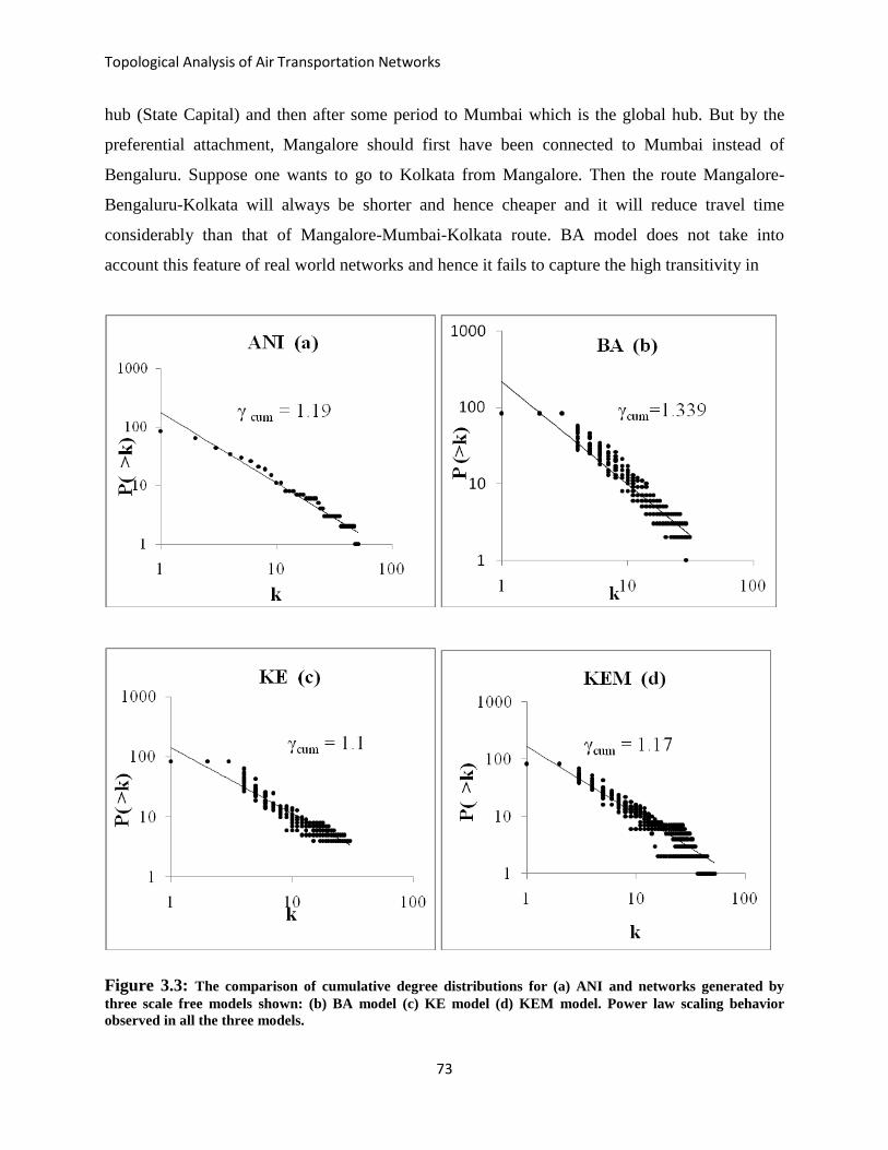
Topological Analysis of Air Transportation Networks
73
hub (State Capital) and then after some period to Mumbai which is the global hub. But by the
preferential attachment, Mangalore should first have been connected to Mumbai instead of
Bengaluru. Suppose one wants to go to Kolkata from Mangalore. Then the route Mangalore-
Bengaluru-Kolkata will always be shorter and hence cheaper and it will reduce travel time
considerably than that of Mangalore-Mumbai-Kolkata route. BA model does not take into
account this feature of real world networks and hence it fails to capture the high transitivity in
Figure 3.3: The comparison of cumulative degree distributions for (a) ANI and networks generated by
three scale free models shown: (b) BA model (c) KE model (d) KEM model. Power law scaling behavior
observed in all the three models.

Topological Analysis of Air Transportation Networks
74
ANI. Thus, by routing flights for new airports through local hubs, the clustering coefficient of
the local hubs is increased (resulting in an overall increase of the average C of the network) and
also leads to shorter path lengths, satisfying both the conditions of high C & low L values of
SWN.
Table 3.1: Network properties of various scale free models implemented with N = 84 and
average degree =3, same as that of ANI.
ANI BA
KE
(µ=0.09)
KE (modified)
(µ=0.65)
C 0.626 0.21 0.621 0.629
L 2.23 2.08 2.289 2.27
P(>k) Power law Power law Power Law Power-Law
γcum 1.19 1.33 1.1 1.17
Degree (Max-Min) 51-1 39-3 41-3 48-2
No. of Hubs 6 2 4 5
Average k 3 3 3 3
Implementation of KE Model
In the BA model, as a consequence of preferential growth, the hubs keep on collecting edges
from new nodes as if there is no limit to the capacity of the node to accept edges. However, in
real life air-transportation network, such as ANI, airports do have limited capacity to connect to
different airports due to limited infrastructure or political plans or geographical constraints.
Airports may run out of space for new runways. Next we implemented Klemm-Equiluz (KE)
model (with its activation and deactivation mechanism) which takes into account this “aging of
nodes” by activating and deactivating the nodes. The data of KE model is averaged over 10
random configurations. The small world behavior is observed in this case by introducing long
range connections, with new node connecting to either the active nodes or to any of the existing
nodes in the network with probability µ. We implemented the KE model, by generating a
network with total number of nodes (84), total number of edges (256) and average degree (m=3)
same as that of actual ANI. For various µ values, we implemented the model, and obtained
networks for 20 configurations for each µ value. We observe from Table 3.2 that for µ = 0.09,

Topological Analysis of Air Transportation Networks
75
the values of clustering coefficient, C = 0.621 and path length, L = 2.28 (calculated for average
of 20 network‟s C and L values.) are closest to that of actual ANI.
Table 3.2: Implementation of KE model for ANI, for N = 84 and m = 3 for different values
of µ giving results of different C and L values.
µ KE Modified KE
C L C L
0 0.760 3.668 0.901 4.050
0.0001 0.696 3.330 0.860 3.775
0.001 0.685 3.003 0.838 3.616
0.01 0.668 2.806 0.788 3.361
0.02 0.658 2.629 0.777 3.223
0.03 0.640 2.531 0.766 3.032
0.04 0.634 2.463 0.756 2.916
0.05 0.632 2.440 0.764 2.873
0.06 0.631 2.365 0.761 2.767
0.07 0.630 2.343 0.757 2.733
0.08 0.626 2.318 0.755 2.719
0.09 0.621 2.289 0.753 2.704
0.1 0.616 2.254 0.724 2.640
0.2 0.598 2.216 0.713 2.555
0.3 0.552 2.152 0.702 2.513
0.4 0.489 2.059 0.692 2.492
0.5 0.429 2.032 0.665 2.428
0.6 0.378 1.996 0.643 2.311
0.65 0.353 1.971 0.629 2.27
0.7 0.329 1.963 0.604 2.163
0.8 0.253 1.933 0.553 2.131
0.9 0.250 1.931 0.548 2.130
1.0 0.205 1.921 0.458 2.110

Topological Analysis of Air Transportation Networks
76
Also, as seen in Fig 3.3(c), the degree distribution of the network (averaged over 20
configurations for µ = 0.09) generated by the KE model follows power law behavior with scaling
exponent value γ = 2.1 (γcum = 1. 1), in agreement with that of actual ANI. Thus, we observe that
for appropriate value of the switching probability, , the KE model incorporates the two
important features of ANI, i.e. high value of C and low value of L. We also observe from Table
3.1 that maximum degree of a node in the network generated by KE model is higher than that of
obtained using BA model. Thus, by incorporating the concept of aging of a node, the KE model
better captures the growth of ANI compared to the BA model. However, in this model,
reactivation of nodes is not taken into account. The hubs are the nodes which have greater than
or equal to the 40% of the maximum degree observed in the network. We see that for BA model,
there are very few number of hubs in the network as compared to that of ANI. However KE
model is in good agreement with that of actual ANI when it comes to the hub structure (Table
3.1). In this case new edges are introduced only through the addition of a new node in the
network. However, in real networks, new links may be introduced even between two existing
(but not connected) nodes to improve the connectivity and traffic flow in the network. In fact, in
an transportation network it is financially and otherwise more easier to introduce new flight-
routes than developing a new airport. We present the results of the KE model with the above
mentioned modification in the next section.
3.3.2 Modeling World Airport Network
On observing the success of the modified KE model in explaining the characteristic features of
ANI, we next carry out the comparative analysis of the scale-free models, namely, BA, KE, and
the modified KE, for a much larger network, the world airport network, WAN. As given in
chapter 2, the WAN considered in this section is constructed by collecting the data for N = 3400
airports. The average degree of WAN is observed to be k = 6 and the total undirected edges of
WAN is 20406. Below we present the implementation details and comparison of the topological
properties of the three model scale-free networks with that of WAN.

Topological Analysis of Air Transportation Networks
77
Figure 3.4: (a) Comparison of degree distributions of WAN and the networks generated by
various model (b) BA (c) KE (d) KEM (2 edges with new node) (e) KEM (4 edges with new

Topological Analysis of Air Transportation Networks
78
node) (f) KEM ( 3edges with new node); with N = 3400 and m = 6. The distributions follow
linear scaling when plotted on log-log scale.
Implementation of BA model
Similar to modeling of ANI, here we first implemented the BA scale free model with preferential
growth to construct a network of the same size (N = 3400), total undirected edges (20406) and
average degree (m = 6) as that of WAN. We start with 15 nodes. The links of the new node are
attached to the existing nodes by preferential attachment. We also observe that the network
follows the scale free degree distribution Fwith exponent value γcum = 1.94 as shown in Fig 3.4
(b). We observe that the clustering coefficient and the characteristic path length are both lower
(C = 0.115 and L = 3.7) than those of actual WAN (C = 0.611 and L = 4.27) (given in Table 3.3).
Table 3.3: The comparison of network properties of actual WAN with the networks
constructed by various scale free models (N = 3400, m =6).
WAN BA KE
(µ=0.04)
KEM-2
(µ=0.07)
KEM-3
(µ=0.08)
KEM-4
(µ=0.1)
C 0.611 0.115 0.612 0.62 0.61 0.612
L 4.27 3.7 3.906 4.19 4.15 4.06
P(k) Power law Power law Power law Power Law Power Law Power law
γcum 1.08 1.94 1.78 1.47 1.57 1.69
Max Degree 280 425 240 365 352
295
Min Degree 1 6 6 2 3 4
No. of Hubs 15 2 4 9 7 6
Implementation of KE model
As in the case of ANI, we observe that the BA model fails to capture the topological features of
WAN. Next we implemented KE algorithm to model the growth of WAN, keeping the number
of nodes (N = 3400), the average degree (m = 6) and total degree as that of actual WAN. We see
that in WAN, the older airports are less likely to increase their connectivity than those added to
the network recently, due to the limitations on space, infrastructure, etc. The KE model
essentially unifies the concepts of small world networks and scale free properties in a single

Topological Analysis of Air Transportation Networks
79
model by introducing a probability µ (to choose between any node or from a set of active nodes
to attach to a new link). We implemented the KE model for a range of µ values from 0 to 1 to
identify at what µ value, a good agreement is observed in the C and L values. These results are
summarized in Table 3.4 on averaging over 20 configurations.
Table 3.4: The values of clustering coefficient and characteristic path length obtained for
the network with N = 3400 and m = 6, with implementation of KE and KEM models for
WAN.
µ KE µ KEM (2
edges with
new node)
µ
KEM (3
edges with
new node)
µ
KEM (4
edges with
new node)
C L C L C L C L
0 0.819 4.893 0 0.838 4.856 0 0.837 4.791 0 0.858 4.913
0.0001 0.760 4.636 0.0001 0.759 4.751 0.0001 0.758 4.684 0.0001 0.779 4.804
0.001 0.700 4.439 0.001 0.730 4.612 0.001 0.729 4.559 0.001 0.750 4.676
0.01 0.671 4.173 0.01 0.690 4.526 0.01 0.689 4.473 0.01 0.710 4.587
0.02 0.641 4.094 0.020 0.667 4.476 0.02 0.654 4.435 0.02 0.671 4.548
0.03 0.621 4.025 0.03 0.651 4.393 0.04 0.640 4.349 0.03 0.661 4.459
0.04 0.612 3.906 0.040 0.649 4.311 0.06 0.631 4.323 0.04 0.651 4.380
0.05 0.612 3.887 0.050 0.643 4.272 0.07 0.628 4.215 0.05 0.641 4.331
0.06 0.602 3.847 0.06 0.641 4.222 0.08 0.610 4.158 0.06 0.631 4.262
0.09 0.592 3.778 0.07 0.628 4.195 0.09 0.602 4.100 0.09 0.621 4.202
0.1 0.572 3.719 0.08 0.613 4.129 0.1 0.597 3.962 0.1 0.612 4.064
0.2 0.552 3.680 0.1 0.592 3.937 0.2 0.581 3.824 0.2 0.602 3.916
0.3 0.513 3.650 0.2 0.582 3.798 0.3 0.571 3.763 0.3 0.592 3.847
0.4 0.474 3.630 0.3 0.572 3.738 0.4 0.551 3.724 0.4 0.572 3.808
0.5 0.424 3.591 0.4 0.552 3.700 0.5 0.522 3.679 0.5 0.543 3.758
0.6 0.345 3.561 0.5 0.523 3.655 0.6 0.482 3.624 0.6 0.503 3.699
0.7 0.286 3.541 0.6 0.483 3.601 0.7 0.444 3.569 0.7 0.464 3.640
0.8 0.247 3.512 0.7 0.444 3.547 0.8 0.394 3.524 0.8 0.414 3.591
0.9 0.241 3.507 0.8 0.394 3.503 0.9 0.384 3.525 0.9 0.404 3.589
1.0 0.187 3.492 1.0 0.252 3.481 1.0 0.233 3.501 1.0 0.385 3.561

Topological Analysis of Air Transportation Networks
80
Figure 3.5: Betweenness distributions of the models BA, KE, KEM implemented for WAN
follow power law when plotted on log-log scale.
The parameter µ here is the crossover parameter to switch between two network models, scale
free and small world. For each value of µ, we generated 20 network configurations and obtained
averaged C and L values. We see from Table 3.4 that clustering coefficient is high in the range 0
< µ < 0.1 for the KE model. For µ=0.04, the model gives scale free degree distribution with the
exponent value γcum = 1.78, as shown in Fig.3.4 (c). This is due to the fact in KE model,
preferential attachment mechanism is maintained when new link is attached to either one of
active nodes or any of the nodes. We also get a high clustering coefficient (C = 0.612)
comparable to that of actual WAN; which is much higher than that of BA. The betweenness
distribution is also observed to follow power law as given in Fig. 3.5. However the KE model is
unable to capture the hub structure in WAN.
3.3.3 Modified KE Model
We observe that the above KE model results in high clustering coefficient and reflects the high
transitivity observed in real scale free networks. This is due to the fact that while adding new
edges from the new node, aging of the node and the long range connections observed in real life
are taken into consideration. However, it may be noted that the new edges/links are introduced
only through addition of a new node the network. While in real network systems, new links may
be added to the existing nodes as well, for e.g. in WWW new links may be added between

Topological Analysis of Air Transportation Networks
81
existing web pages. This is especially true in the case of transportation networks, wherein new
rail tracks, new routes are added among existing stops/ports. This feature is not taken into
account in the BA or KE models. Here we propose a modified form of KE model by
incorporating this additional feature and investigate the properties of this model with respect to
ANI and WAN. In KE model, every new node adds number of links which is equal to the
average degree of the network. If m is the average degree, then at every iteration, then a fraction
of m links come from the new node (as in the case of KE model), while the remaining fraction of
(1-m) links are introduced between the existing nodes chosen by preferential attachment. The
activation and deactivation of nodes as proposed in the KE model which limits the capacity of a
node to grow is also taken into account. Using crossover parameter, this model also exhibits a
network with high clustering coefficient and small characteristic path length. The clustering
coefficient is high for almost the entire range of the crossover parameter, µ, in this case. For µ =
1 the KE model approaches the BA network and the small-world properties are lost. However in
the modified KE model, as new edges are added among existing nodes at every iteration, high
transitivity is maintained even at µ close to 1.
Implementation of Modified KE Model for ANI
Though the KE model agrees very well with most of the properties of actual ANI, it may be
noted in Table 3.1 that the maximum degree in ANI is higher than in the KE model, and also the
number of hubs are fewer in the KE model compared to ANI. In airport networks, we know that
new flight routes are continuously developed among existing airports as the cities are developed
financially or gain political importance over time. We implemented the modified KE model, with
N = 84 and total undirected edges = 256. At every iteration, in this case we added a new node
with degree 2 and added one edge among existing nodes, maintaining the average degree of ANI
(m = 3).
It may be noted from Table 3.1 that in the case of modified KE model, the value of for which
the C and L values are in agreement with that of ANI is much higher than the original KE model,
µ = 0.65: C = 0.629, L = 2.27. The modified KE model with high clustering coefficient and low
path length exhibits small world behaviour. Also, it may noted in Fig 3.3 that there is a very

Topological Analysis of Air Transportation Networks
82
good agreement in the degree distribution of this network with actual ANI, with scaling exponent
γ = 2.07. It also exhibits hub structure with maximum number of hubs observed in this network
being 5, in good agreement with actual ANI compared to BA and KE models. Thus, it may be
noted that the proposed modification of the original KE model captures very well the actual
nature and evolution of ANI.
Modified KE Model for WAN
In both KE and BA model, we assumed that new edges just appear with inclusion of new node in
the network. However in real network systems, new links are added continuously. We
incorporated this feature in the KE model, referred to as Modified KE model here after, by
introducing new links among existing nodes apart from those introduced with the new node. We
simulated three variations of the modified KE model where the ratio of the fraction of m edges
are introduced by the new node and among the existing nodes differ. This is done to analyze the
effect of introducing new links between existing nodes and how the topological properties differ
compared to the KE model. The three situations considered are: (1) Four edges are introduced
with the new node and two among existing nodes (KEM-4), (2) Three edges are introduced with
the new node and three among existing nodes (KEM-3), and (3) Two edges are introduced with
the new node and four among existing nodes (KEM-2). Three model networks are constructed
having total number of nodes and edges and the average degree the same as that of WAN.
First we consider the case when 4 edges are added with addition of new node to the existing
nodes. At the same time, two edges are added among existing nodes by preferential attachment.
For different values of µ we constructed 20 network configurations. From Table 3.4 we identify
the value of µ = 0.1 for which the values of C (0.612) and L (4.06) are in closest agreement with
that of actual WAN. The high value of clustering coefficient and low value of path length
indicates that the network is small world. The network follows power law scaling with the
exponent value γcum = 1.72, shown in Fig 3.4 (f) (obtained for 20 network configurations).
We then simulated the model by changing the percentage of distribution of links among new
node and among existing nodes. We observe from Fig 3.4 (d) and Fig. 3.4 (e) that the networks
generated by modifying the distribution of edges in KEM model, also have degree distributions

Topological Analysis of Air Transportation Networks
83
which follow power law with γcum = 1.57 for KEM-3 and γcum = 1.47 for KEM-2 models
respectively. Also, the clustering coefficients and the characteristic path lengths have also been
confirmed in accordance with WAN (From Table 3.3).
We see that the minimum degree of the network gets closer to the actual WAN (i.e. 1) when we
add 2 edges with the new node. In real situations one would expect that when a new airport is
added, it is likely to be connected to one or two existing nodes in the network. It gets connected
to more airport over time. This feature is incorporated in this model. The maximum degree of the
hub in this model is closer to that of WAN than BA and KE models (Table 3.3). In WAN, the
nodes which are capital of the countries, are connected to most of the other capitals that means in
WAN, many hubs are connected to many hubs (high degree nodes). This results into the
development of number of global hubs in WAN. However in the modeling part, this feature is
not taken in account. In the model, the most connected nodes are also the central nodes in the
network and the anomaly is not observed as in case of real WAN. We have been able to see hub
structure in all the variations of KEM model however it is not in good agreement with WAN.
The hubs are defined as the nodes having greater than or equal to 40% of the maximum degree
observed in the network. From Table 3.3, we observe that when more edges are distributed
among the existing nodes, the network reflects better hub structure. (Maximum hubs are
observed for the case when four edges are distributed among the existing nodes.)
We observe that the hub structure is depicted by the KEM models. We next analyze the
distribution of betweenness centrality in these models. The betweenness distributions of these
networks are seen to exhibit power law behavior as seen in Fig. 3.5 (γcum = 0.709, 0.723. 0.711
for KEM-2, KEM-3, KEM 4 respectively), in agreement with that of actual WAN. This indicates
that there are few nodes with very high betweenness values and most of the nodes have very low
betweenness values. However, the anomaly in the centrality measures observed in actual WAN
is not observed in any of these models. In WAN, the finding of central nodes with low degree is
and intrinsic property of WAN. The reason behind the betweenness anomaly observed in WAN
is related to various factors such as geographical/geological locations of the airport, economical
growth and political relations between countries and mainly the large distances between airports
which are in different continents. The degree betweenness anomaly is related to the existence of
Topological Analysis of Air Transportation Networks
84
communities (that are formed because of the mentioned factors in different continents) in the
network. However, in the models, we did not take into account these factors. We find the most
connected nodes are always most central.
This modified form of the KE model thus reproduces most of the empirical and structural
observations for both ANI and WAN. We have taken into the account the very intrinsic property
of these networks and that is these networks are not stationary or static with fixed topology.
However their structures evolve and new links and nodes continuously appear. Such topological
fluctuations influence on the dynamics of these networks.
In an overview, we observe that the regular Barabasi-Albert fails to explain high clustering
coefficients observed in both the transportation networks: ANI and WAN. The discrepancy is
mainly due to the fact the in real networks, when the new node is added, the attachment of its
link is not due to the preferential attachment only (i.e. to the links that the node already has) but
other factors such as geographical distance, cost of building the new airports, airline policies,
political importance, geographical location (hill stations), etc. affect the introduction of new
airports and flight routes. This transitivity of the real life networks arises due to the attempts to
reduce the travel cost and time and improve the connectivity by reducing the hop count.
We observed that KE model is more suitable model than BA model as it takes into account the
high transitivity and aging of the nodes, while generating a scale free distribution. However, it
does not take into account the reactivation of the nodes. Also, in real transportation networks,
newly added node gets attached to the local hub (geographically) than any global hub in the
network. We incorporated this factor in modified KE model and observe good agreement in
major topological properties of both ANI and WAN. Thus, formation of new links among
existing nodes, as the network evolves, is a crucial point in terms of evolution of network.
However we know that there are certain limitations to the model. As proposed in chapter 2, we
observed that newly added nodes attach to local hub than global hub. This can be taken into
account if we actually consider the geographical co-ordinates of the places. The anomalous
centrality behavior which was observed in WAN was not observed in any of the models
implemented. This is the intrinsic property of WAN which incorporates the large geographical

Topological Analysis of Air Transportation Networks
85
area over which WAN is spanning, and also the political constraints and policies. Inclusion of
some of these points would help us model the transportation networks in more realistic ways.
CHAPTER 4
SIR Model of Infectious Disease
4.1 Introduction
Many infectious diseases spread through populations via the networks formed by physical
contacts among individuals. The advent of modern transportation has speeded up disease
transmission significantly. We have observed that infectious disease like Avian flu, SARS,
spread rapidly across the world within a very short time and became pandemic (Meyers et al,

Topological Analysis of Air Transportation Networks
86
2004). The reason behind this is the densely connected transportation systems. We have
observed in the previous chapters that WAN and ANI, both have very high clustering and are
well connected with a very short characteristic path length. We have observed that crucial
airports in these scale free networks, termed as “hubs”, not only have high connectivity but the
airports manage a heavy traffic flow with large number of flights. Obviously, there stands a
higher chance of spread of disease in such cities. To analyze the spread of infectious disease
through such scale free and small world networks, we first study if there is any relation between
the number of cases reported in particular city and the connectivity of that city. By analyzing the
recent spread of influenza H1N1, 2009, we observe from Fig 4.1 (a) that correlation between
number of passengers arriving from Mexico to different countries in WAN and the number of
swine flu cases reported in those countries is very high, (r =0.93). Here only direct flights from
Mexico are considered. Similarly, assuming Delhi as the origin of spread of swine flu in India,
number of flights from Delhi and number of swine flu cases in the cities in India also shows a
high correlation with correlation coefficient, r = 0.84 (Fig. 4.1(b)). The strong correlation
indicates that improved connectivity in transportation networks does increase the rate of spread
of disease, and disease becomes endemic and then pandemic in a very short time. Therefore,
modeling of spread of epidemics through transportation networks has played a vital role in
predicting the impact of a disease. We have observed that both WAN and ANI are scale free
networks with small world characteristics. It has been proposed that structures of such complex
networks may underlie fast transmission of infectious agents within various communities.
Despite a lack of direct experimental evidence supporting this hypothesis, a number of
theoretical studies have shown that topological structures typical of complex networks (in
particular, scale-free and small-world topologies) lead to transmission dynamics markedly
different from that predicted by standard disease transmission models (Newman, 2002). These
models try to answer the questions such as will a certain disease be an epidemic or what
percentage of the population will be affected or what percentage will die etc. These models
suggest that if the transmissibility of the pathogen is lower than some threshold, the disease will
terminate. Recent studies of infectious agents (computer viruses or biological pathogens) in
certain complex networks have shown that in these networks such a threshold does not exist. In
particular, if the connectivity within a network follows a scale-free distribution and the
transmissibility of the agent is positive, then an epidemic is inevitable. Only if the recovery from

Topological Analysis of Air Transportation Networks
87
the infected state confers immunity, an epidemic is inevitable only if the population is infinite. If
a disease is spreading on a scale-free network, then eradication of that disease is only possible if
transmission is reduced to precisely zero. (It has been shown if 1 < γ ≤ 2, then this distribution
does not have a finite mean. Even if 2 < γ ≤ 3 the variance of the number of links is infinite and
therefore even with very small (but nonzero) rate of transmission, transmission will still persist
(Small et al, 2007).
In this chapter, we simulate the spread of disease in the transportation networks (ANI and
WAN), considering a well known mathematical model (SIR). We explain this standard
“Susceptible-Infected-Recovered Model” (SIR) first and analyze the spread.
Figure 4.1: (a) The correlation between number of passengers arriving from Mexico in
various countries in WAN and the H1N1 cases reported in those countries, with correlation
coefficient = 0.93. (b) The correlation observed between number of cases of swine flu H1N1
in India and the number of flights from Delhi is 0.84.
4.2 SIR model
In recent years large-scale computational models for the realistic simulation of epidemic
outbreaks have been used. Methodologies range from very detailed agent based models to
spatially-structured metapopulation models. Many traditional epidemiological models implicitly
contain the assumption of homogeneous mixing which means that all nodes in the network
connect each other with equal probability. This condition does not hold true for the
transportation networks which we are considering. We consider a sample compartmental model
– SIR model on the air transportation networks which is used for the network with heterogeneous

Topological Analysis of Air Transportation Networks
88
connectivity and then implement it on ANI and WAN to observe the spread of disease through
these networks.
To model the spread of disease in the large population comprising many different individuals,
the diversity in the population must be reduced to a few key characteristics which are relevant to
the infection under consideration. Compartmental models divide the population into subclasses
known as compartments. In SIR model as expressed in Fig.4.2; the population is divided into
three compartments, susceptible (S), infected (I) and recovered (R). A susceptible individual in
contact with an infectious person contracts the infection at rate β. What qualifies as a contact
depends on the disease. Each infected individual remains infectious for a mean infectious period,
denoted as μ-1
. After the mean infectious period, infectious individuals recover permanently. The
model is dynamic in the sense that numbers in each compartment may fluctuate over time. A
single epidemic outbreak can be studied by this model by neglecting birth-death rates, and in that
case, SIR system is expressed by the following set of ordinary differential equations:
4.1
4.2
4.3
It is assumed that the rate of infection and recovery is much faster than the time scale of births
and deaths and therefore, these factors are ignored in this model. This model was for the first
time proposed by O. Kermack and Anderson Gray McKendrick. This system is non-linear, and
does not have a generic analytic solution (Kermack and McKendrick, 1927).
It can be also noted that
4.4
it follows that:
S(t) + I(t) + R(t) = Constant = N 4.5

Topological Analysis of Air Transportation Networks
89
expressing in mathematical terms the constancy of population N.
Figure 4.2: Compartmental Model for SIR
This is a very simplistic approximation of SIR. There is a threshold quantity which determines
whether an epidemic occurs or the disease just dies out with time. This measure is termed as the
basic reproduction number, denoted by R0, which is defined as the number of secondary
infections caused by a single infective introduced in a population made up completely of
susceptible individuals (S(0) ≈ N) over the course of the infection of this single infective. This
infective individual makes β*N contacts per unit time producing new infections with a mean
infectious period of 1/µ. Therefore, the basic reproduction number is
R0 = (β*N)/µ 4.6
This ratio is derived as the expected number of new infections from a single infection in a
population where all subjects are susceptible. The basic reproduction number R0 is the number of
secondary cases which one case would produce in a completely susceptible population. It
depends on the duration of the infectious period, the probability of infecting a susceptible
individual during one contact, and the number of new susceptible individuals contacted per unit
of time. Therefore R0 may vary considerably for different infectious diseases but also for the
same disease in different populations. If R0 = 1, the disease becomes endemic. This means that
the disease exists in the population at a consistent rate, as one infected individual transmits the
disease to one susceptible (Dietz K, 1993).
4.3 Results and Discussion
The SIR compartmental model discussed above divides the population into three compartments:
susceptible, infected and recovered. For simulation of SIR model on air transportation networks,
we have considered the airports in the air-networks as nodes and connectivity between them as

Topological Analysis of Air Transportation Networks
90
edges. We first infect few nodes (airports) in the network and mark these nodes as infected and
rest of the others as susceptible. At every iteration, we infect only the neighbors of the infected
nodes that are susceptible, with some threshold rate of infection. (Neighbors are those airports
which are connected to the infected node with the direct flight). In this way, we observe the first
occurrence of infection in the nodes of such network. Here the population size is constant, which
is the total number of airports in the network. In this simulation, a recovered node will not get
infected again. That is effectively, there is no R state in our implementation as there is no
concept of immunity in case of airports. Any airport in the network has some chance of getting
nfected again and again as long as it is connected to the nodes in the network. Therefore,
effectively the model is now SI model. We present the analysis of the spread can be restricted on
looking at different initial conditions.
In our SIR model, we have defined two parameters, viz. rate of infection (β) and rate of
recovery (µ). Throughout the implementation, we have assumed that the rate of recovery
is zero so that once the node is infected; it continues to infect its neighbours with fixed rate
of infection. We analyze the spread of infection through ANI with varied rate of infection
(β) in Fig. 4.3. over the period of 100 days. As expected with high infection rate β , the number
of infected individuals is higher. The saturation value for β = 0.1 is the maximum in the three
cases and it is reached in shortest time period among the three. We fix the rate of infection as
0.05 throughout our further simulations.

Topological Analysis of Air Transportation Networks
91
Figure 4.3: The spread of infection in ANI for different rates of infection, β, shown.
In chapter 2, we have observed the fall in the efficiency of ANI and WAN when the connections
from major nodes were removed from the network. We expect that the spread of infection to be
lower if such important nodes (based on their centrality measures) are removed from the network
and the spread would be faster if such nodes get infected at the earlier stages. Here we analyze
the spread of infection on air transportation networks in two situations. 1. Choosing nodes for
initial infection. 2. Analyzing spread of infection after removing high centrality nodes in the
network. We select the nodes based on the centrality measures and compare the results with
randomly chosen nodes.
4.3.1. Choosing nodes for initial infection
ANI has been observed to be a scale free network. In chapter 2, we have observed that 6 major
hubs (based on their centrality values viz. Betweenness, closeness and degree) exist in ANI. In
Table 4.1, we have compared the spread of infection when different nodes are initially infected.
When all these six hubs are infected at once as the intial condition, in Table 4.1; we have shown
the maximum number of nodes in the network getting infected and we analyze T1/2 i.e.the time
period in which half of the nodes in the network get infected. We compare the results when
randomly chosen nodes are infected. All the randomized values are averaged over 20
configurations. In Fig.4.4, we have plotted the number of nodes getting infected (first instance of
infection at the airports) when various hubs are initially infected.
Table 4.1: Comparison of spread of infection when different nodes are initially infected.
Initially infected nodes Max number of infected
nodes in the network
T1/2
Delhi 54-76 7-11
Mumbai 57-72 7-12
Kolkata 49-63 8-14
Bengaluru 52-65 8-13
Chennai 55-63 9-16
Hyderabad 54-64 9-16
Delhi and Mumbai 58-77 4-7
B’lore+Chen+Hyd 60-72 5-6
6 hubs 68-84 2-6
6 random nodes in ANI 43-71 10-15

Topological Analysis of Air Transportation Networks
92
6 random nodes from
randomized ANI
38-61 12-16
We see from Fig 4.4 that within just 8 days, the infection is spread all over the network with all
the 84 nodes getting infected. On the contrary, when we randomly infectd 6 nodes from ANI and
then analyzed the effect of the spread on the network, we observed that the saturation point is
reached on 18th
day and the maximum number of infected nodes are 3/4th
of the total number of
nodes. The saturation point is smaller in this case. In the case of random infected nodes 50% of
the nodes are infected at 11th
day while when the hubs were infected, T1/2 was just 3 days, when
50% of the nodes got the infection (Table 4.1). This is due to the scale free nature of ANI.
Previously, in chapter 2, we have shown the effect on efficiency of ANI after removing the hubs
is higher than that of removing the random nodes. Here we show that although hubs are very
important in maintaining the connectivity of ANI, they have a negative effect of propagating
disease very fast in the network.

Topological Analysis of Air Transportation Networks
93
Figure 4.4: Trend of infected nodes with error bars in ANI when different nodes are
infected at initial iteration.
If the hubs get infected, then the spread of the disease through network is faster than if the
infected nodes at initial iteration are randomly chosen nodes. Also, when we checked the spread
on randomized network of ANI by infecting 6 randomly chosen nodes, we observed that the
spread was slower compared to all the cases in ANI.
WAN, compared to ANI is a much complex network with a large number of vertices and edges
among them. We have analyzed properties of WAN in chapter 2 and we have shown that WAN
is a scale free network with small characteristic path length. We next simulated the SIR model on
WAN and analyzed the results for various initial conditions. From Fig 4.5, we observe that when
initially 15 random nodes were infected (0.5% of total nodes in WAN), then around 500 nodes
got infection within 12 days and it remained saturated (all the randomized values are averaged
over 20 configurations). However when we infected 15 hubs (chosen according to their degree
values), we observe a steep curve. Out of 3400 nodes in WAN, 3290 nodes got infected within
20 time steps. It indicates that these hubs have huge impact in the efficiency and connectivity of
ANI, and hence the spread of disease is faster through these airports once they get infected. Next,
we checked the impact on the spread of disease when we infected only one airport, London, in
the first iteration. This airport is an important hub in Europe, and also on global scale; mainly
because it connects the continents Asia and America. Once it is infected, within less than 10 time
steps, the disease spread over 1000 nodes in the network i.e. the impact is double of infecting 15
random nodes. We analyzed the impact of initially infecting London along with another major
hub, Frankfurt. For 10 time steps, the infection spread is almost similar to that of infecting 15
hubs. After 10 days the number of infected nodes saturates at around 1800 nodes; much lesser
than that of infecting 15 hubs.

Topological Analysis of Air Transportation Networks
94
Figure 4.5: Trend of infected nodes in WAN with different initial conditions
4.3.2 Removal of Node
Scale free networks are robust against removal of random nodes. However, the connectivity
collapses when the hubs are attacked. To contain the disease spread, we would like to reduce the
connectivity and efficiency of the network.
Table 4.2: Number of infected airports in eastern and southern India with and without
removal of Kolkata and Chennai.
Day Without
removal of
Kolkata
With removal
of Kolkata
Without
removal of
Chennai
With
removal of
Chennai
1 0 0 0 0
2 0 0 0 0
3 1 0 1 0
4 2 0 1 0
5 2 0 2 0
6 3 0 3 1
7 4 0 3 1
8 4 0 4 2
9 5 0 5 3

Topological Analysis of Air Transportation Networks
95
10 5 0 5 3
11 5 0 6 4
12 7 1 7 5
13 8 1 7 6
14 8 1 8 7
15 8 2 9 7
16 8 2 10 8
17 8 3 11 9
18 8 4 11 10
19 9 4 12 10
20 9 4 12 10
21 9 5 12 11
22 9 5 13 11
23 9 6 13 12
24 9 6 13 12
25 9 6 13 12
When infected cases are found in one city, to restrict the spread of disease to other cities through
human contact, we need to isolate that city from the rest. By removing one of the important
nodes in ANI, we want to investigate whether it is possible to restrict the spread of disease in the
vicinity of the node removed. We removed Kolkata from ANI, (i.e. removed all the links to and
from Kolkata) and then simulated the SIR model (Fig. 4.6). We expect the eastern region of
India to be either completely restricted from getting infection or a significant delay in these
airports getting infected. In Table 4.2 is shown the simulation on removal of two hubs in ANI.
We observe from Table 4.2 that when we initially infected Delhi and simulated the results by
removing the node Kolkata, on the 12th
day one of the airports in eastern India got infected.
When we did not remove Kolkata, more than 50% of the nodes in eastern India got infected
within 10 days. However when Kolkata was removed, it took almost two and a half weeks to
spread the infection to 50% of the nodes. We observed that by 23rd
day, 6 of the airports in
eastern part got infected and the infection is saturates as out of 8 airports in eastern India, two
airports have connections only to Kolkata. So when Kolkata is cut off, those two airports are cut
off from rest of ANI, and there is no path through which they could get the infection. When we
did not remove Kolkata, on the third day itself one of the airports in eastern India got infected
and within 9 days most of the airports in eastern India obtained the infection. In Fig. 4.6; we
show the spread in eastern India when Kolkata is removed from ANI. However, when we

Topological Analysis of Air Transportation Networks
96
removed Chennai from ANI, which is one of the major hubs in southern India, we did not
observe similar scenario. With or without removal of Chennai, within 3-6 days, one of the
airports in southern India gets the infection and the spread is almost the same (Table 4.2). This is
because there are three local as well as global hubs in southern India, and these share more than
50% of destinations among themselves. So even when Chennai is removed, once either
Bengaluru or Hyderabad (the other local hubs in southern India) gets the infection then the
spread in southern India is quite fast. Although the connectivity and overall network efficiency
improves by having more than one local hubs, in the case of disease spread, this has the adverse
effect. When all the 6 major hubs in ANI are removed, we observed that network is not
connected and hence the spread of infection is low. However in case of WAN, we observed in
chapter 2 that due to anomalous behavior of centralities, top 15 nodes in each of the centrality
measures vary. We remove top 15 nodes based on their centrality values, and then analyze the
spread of disease by initially infecting 15 nodes chosen at random. We observe from Fig. 4.7 that
when we remove top 15 nodes with high closeness value, maximum number of nodes get
infected. The trend of disease spread is similar, but slightly lower for removal of high-degree
nodes (~ 645) followed by removal of high closeness nodes (~ 755). This is because almost 10
nodes among top 15 high centrality nodes are common in each case.

Topological Analysis of Air Transportation Networks
97
Figure 4.6: Infection spread in Eastern India when connections from Kolkata are removed.
(a) Inititial condition, day = 0 (b) day = 13 (c) day = 16 (d) day = 25.
When we removed 15 nodes randomly from the WAN, then the spread was much higher than
other three cases when nodes were removed based on their centrality values. This is because
those randomly chosen nodes may be the nodes with very low centrality values and their
connectivity could be very low. Removal of such nodes does not affect efficiency in case of scale
free networks. Only when some of the hubs in the network get infected, then the infection
spreads faster. This analysis demonstrates the impact of removal of high-centrality nodes on
disease transmission in air-transport networks.

Topological Analysis of Air Transportation Networks
98
Figure 4.7: Trend of number of nodes getting infected after removal of nodes in WAN
based on their centrality measures.
Removal of flights from weighted ANI
It is practically impossible to close down airports to restrict the spread of disease as this would
involve huge financial losses for airline companies and a lot of inconvenience for passengers
travelling across the globe. Instead of removing nodes completely, we can identify important
edges where the traffic density is high; the cancellation of flights on such routes may help in
delaying the spread of disease if not in completely containing it. In ANI, we observe that Delhi-
Mumbai route is the busiest route with 120 flights per day, and Delhi-Bengaluru is another busy
route with 64 flights per day. We identify 15 such routes (out of total 256) with number of
flights/per day > 40 and reduce the number of flights on such paths. In Fig.4.8 we have shown
the comparison of spread of disease when top flights from top 15 busiest routes are reduced and
when the 6 hubs are removed. We see from Fig 4.8 that when 6 hubs are removed from the
network, the network breaks down into clusters and the disease spread is very low. Not even half
of the nodes in ANI get the infection. Although selective removal of hubs reduces the spread

Topological Analysis of Air Transportation Networks
99
considerably, it is not feasible to remove nodes with such a high importance from ANI or from
WAN.
Figure 4.8: Comparison of spread of the disease in weighted ANI when flights (weights) on
top 15 busy routes are removed and when 6 hubs are removed.
From Fig 4.8 we observe that the spread of disease on weighted ANI, when 6 nodes are infected
initially at random, is high and more than 70 nodes are infected. However when the weights on
the edges are removed, the spread is slower. When randomly six nodes are removed, T1/2 for
weighted ANI is less than 10 days while when we removed 50 % of flights on the 15 routes, T1/2
is 15 days. For 100% removal of flights routes on these 15 edges, T1/2 is further delayed and is
more than 20 days. We observe that the impact after removing all the flights on just 5% of edges
is almost similar when we remove 6 hubs out of 84 nodes (~7% of nodes) in the network. This
simulation study shows that reducing flights on selected busy air-routes is one of the quick and
effective control strategies in case of spread of diseases. Also, removal of selected edges is easier
compared to complete closure of the airports.

Topological Analysis of Air Transportation Networks
100
In today‟s world, with a large number of passengers traveling around the globe, infectious
diseases may spread rapidly around the world and become severe threat to the society. Global
epidemic forecast would therefore be extremely relevant in the case of the emergence of a new
pandemic influenza. We believe that our analysis of the airport network represents a reference
point for the development of efficient strategies to prevent spread of diseases.

Topological Analysis of Air Transportation Networks
101
CHAPTER 5
Conclusion
In this thesis we have analyzed the topological properties of two air transportation networks,
airport network of India (ANI) and world airport network (WAN) using graph theoretic
approach. Air networks appear unique and extraordinary due to following reasons: a) limited
size b) Bi-directional weighted edges (flights) and c) stationary structure. In chapter 2, we have
given a detailed analysis of structural and topological properties of ANI and WAN. Through the
study of airport network of India (ANI), composed of 84 airports and 512 direct edges, we
showed that topological structure of ANI conveys two characteristics of small worlds, a short
path length and a high degree of clustering. The cumulative degree distribution of ANI obeys
powers law describing its scale free nature in agreement with earlier study by Bagler, 2008. In
our analysis of ANI, we observed that the most connected cities also have high values for other
centrality measures, Betweenness and Closeness. A review of airport networks of various
countries such as China, Italy, Brazil, Austria, and U.S. showed that ANI shares many features
common to these networks, most notably the small world and scale free behaviour. The main
contribution of this thesis is the analysis of centrality measures. The questions we have tried to
address here are (1) how such an analysis can help in increasing the efficiency of the network to
reduce the time and cost of travel, (2) what is the impact of targeted versus random removal of
nodes/edges on the efficiency, integrity and stability of the network, and (2) the role of the
critical nodes in the event of undesirable situations, e.g., weather conditions, epidemic situations,
etc.
In our analysis of centrality measures, as shown in Chapter 2, these not necessarily be the ones
with high connections but may also be the ones lying on high traffic-routes (high betweenness)
or geographically well distant nodes (closeness). By simulation study we show that even though
some small airports like tourist spots, IT cities, and historical places have very few connections,
if they have just one connection to one of the major hubs in the network, it helps in improving
their closeness value. This definitely would add up to the revenue generated as the airport
becomes easily accessible by any other nodes in the network. Being a scale free network, ANI is

Topological Analysis of Air Transportation Networks
102
resilient against random attacks; however, efficiency remarkably decreases if the hubs are
removed. We also analyzed the weighted ANI where weights are proportional to the number of
flights. Instead of removing the connection from two nodes completely, if we reduce number of
flights on the important route, that reduces the flow of traffic without losing the connectivity.
This strategy is helpful when we need to contain the spread of disease, as otherwise complete
close down may result into huge financial loss. We also proposed that presence of two or more
local hubs helps in improving the efficiency and even though the network is scale free,
connectivity does not fall down in case of accidental failure of one of the hubs. This further
helps plan suitable locations for establishing new hubs.
The importance of WAN goes beyond the convenience it provides to the world travelers. We
observed that like ANI, WAN, consists of 3400 airports and 56,749 direct flights. Graph
theoretic analysis of WAN suggests that it is a scale free network with small world nature in
agreement with earlier studies. However, unlike ANI, the most connected nodes in WAN are not
necessarily central. We observed the anomalous centrality behavior of WAN for both
betweenness and closeness. These anomalies are due to the multi-community structure of WAN.
We then analyzed centrality measures of WAN and take up particular case study of volcanic ash
eruption in Europe in April, 2010. Due to the cancellations of flights at European airports, the
delay percolated to other airports in the world, causing delays at the world‟s top hubs. We
investigated how the strength of airports was affected due to the calamity and provide
suggestions on how one could manage traffic in such situations in future. Another issue
addressed here is the efficiency of WAN. Unlike in the case of ANI, removal of a single node do
not show significant drop in the efficiency. Being a larger network than ANI, many alternate
paths exist in WAN. We analyzed the efficiency of WAN on removal of edges from top 10 nodes
chosen according to their centrality values. We found that on 100% removal of edges, (which is
equivalent to the removal of the node), the efficiency drops to almost two third of the original
efficiency when the nodes are removed based on their betweenness value. No such drastic fall is
observed in case of random removal of nodes.
To understand the evolution and growth of these transportation networks, we next analyzed
various scale-free models to see which best explains their growth. Though both ANI and WAN
exhibit scale free properties, the most popular scale-free model, proposed by Barabasi and Albert

Topological Analysis of Air Transportation Networks
103
fails to explain the evolution of these transportation networks. The discrepancy is mainly due to
the fact the in real networks, when the new node is added, the attachment of its link is not due to
the preferential attachment only (i.e. to the links that the node already has) but other factors such
as geographical distance, cost of building the new airports, airline policies, political importance,
geographical location (hill stations), etc. affect a lot on the attachment. While analyzing the
network properties of various scale-free models, we observe that these fail to explain high
clustering coefficient observed in ANI and WAN. This high transitivity of the real life networks
arises due to the attempts to reduce the travel cost and time and to improve the connectivity by
reducing the hop count. We noted that among various models studied, the Klemm-Eguiluz model
generates a network which exhibits both scale-free and high clustering coefficient, small-world
behavior. We observed that in real networks new links are continuously added and not just with
the inclusion of new node. Links are formed among existing nodes and networks evolve with
time. Here we proposed a modification of the Klemm-Eguiluz model to incorporate this feature
of real transportation network and observed that most of the properties of the network generated
by our proposed model are in very good agreement with those of actual ANI and WAN.
One of our important goals for analyzing these transportation networks was also to understand
the spread of infectious diseases through these networks. It has been observed that densely
connected air-transportation networks play a major role in the spread of infectious diseases, viz.,
Avian-influenza, Swine-Flu, etc., turning from epidemic into pandemic in a short interval of
time. Knowledge of the connectivity pattern and load on various routes can help in making
judicious decisions for reduction of flights to contain the spread of the disease. By analyzing
these two transportation networks, one at national level and the other at international level, we
observe that structure of these networks can only be understood in terms of geographical,
financial and political considerations. It is clear from the study that in the reality of air
transportation, the carriers (airlines) should consider more factors in order to have a higher and
reasonable efficiency. However, to contain the spread of disease, one needs to know how an air
network can satisfy the passengers‟ needs on one hand, and reduce spread through a network
which is efficient on the other hand. To show the effect of the underlying topology on the spread
of infectious diseases, we implemented the simplest SIR compartmental model on both ANI and
WAN. As expected, we observed that the impact of the spread on the network when initially the

Topological Analysis of Air Transportation Networks
104
hubs are infected is higher than when random nodes are infected. To restrict the spread of
infection on the network, we show that instead of closing down of airports with high centrality
value, we could achieve similar delay in disease transmission by reducing the flights on
important routes. We show that cancellation of flights is a better strategy to contain the spread of
disease in agreement with the results in Chapter 2.

Topological Analysis of Air Transportation Networks
105
BIBILOGRAPHY
Albert R and Barabasi A L.,“Statistical Mechanics of Complex Networks [J]”, Reviews of
Modern Physics, 74(1), 47−97 (2002).
Amaral L.A.N, Scala A., Barthelemy M. and Stanley H.E. “Classes of Small World
Networks”, PNAS, doi:10.1073/pnas.200327197, 11149-11152 (2000).
Antoniou E. and Tsompa E., “Statistical Analysis of Weighted Networks,” Discrete
Dynamics in Nature and Society, vol. Article ID 375452, 16 pages,
doi,10.1155/2008/375452 (2008).
B S Cooper, “Delaying the international spread of pandemic influenza”, PLoS Med. 3 e12
(2006).
Bagler G., “Analysis of airport network of India as a complex weighted network.”
Physica A.387 2972–2980 (2008).
Barabasi A.-L. and Albert R., “Emergence of scaling in random networks.” Science Vol.
286. 509–512 (1999).
Barrat A., Barthelemy M., Pastor-Satorras R. and Vespignani A., “The architecture of
complex weighted network” , Proc. Natl. Acad. Sci. (USA) 101(11) 3747–3752 (2004).
Berger A., Muller-Hannemann M., Rechner S. and Zock A., “Efficient computation of
time-dependent centralities in air transportation networks.” LNCS. 6552. 77-88
WALCOM (2011).
Caldarelli G., Capocci A., De Los Rios P. and Munoz M., “Scale-free Networks without
Growth or Preferential Attachment, Good get Richer”, Nature, arxiv preprint cond-
mat/0207366, (2002).
Colizza V, Barrat A, Barthelemy M, Vespignani A., “Predictability and epidemic
pathways in global outbreaks of infectious diseases, the SARS case study”, BMC
Medicine 5,34. (2007).
Colizza V, Barrat A, Barthélemy M, Vespignani A., “The role of airline transportation
network in the prediction and predictability of global epidemics”, Proc Natl Acad Sci
(USA), 103,2015-2020 (2006).

Topological Analysis of Air Transportation Networks
106
Derenyi I, Palla G, Vicsek T., “Clique percolation in random networks [J]”, Physical
Review Letters, 94(16), 160202 (2005).
Dijkstra, E. W. "A note on two problems in connexion with graphs". Numerische
Mathematik 1: 269–271. doi:10.1007/BF01386390 (1959).
Dorogovtsev S N, Mendes J F F, Samukhin A N., “Structure of growing networks with
preferential linking [J]”, Physical Review Letters, 85(21), 4633−4636 (2000).
Dorogovtsev, S. N. and Mendes J. F.M., “Scaling properties of scale-free evolving
networks, Continuous approach”, Physical Reviews E 63, 056125, arXiv,cond-
mat/00120 (2001).
Erdos P. and Renyi A., “On Random Graphs I”, Publ. Math. Debrecen 6, 290 (1959)
Guida M. and Funaro M., “Topology of the Italian Airport Network”, Chaos, Solitons &
Fractals, Vol. 31, p.p. 527-536 (2007).
Guimera R., Mossa S., Turtschi A. and Amaral L. A. N., “The worldwide air
transportation network, Anomalous centrality, community structure and cities‟ global
roles.” PNAS. Vol. 2 7794–7799 (2005).
Guimerà, R., Mossa S., Turtschi A., and Amaral L., “Structure and Efficiency of the
World-Wide Airport Network”, arXiv,cond-mat/03125, PNAS,Vol 1, 19 Dec (2003)
V. Batagelj , A. Mrvar “ Pajek – Program for Large Network Analysis”, Connections,
21,2, 47-57, (1998) http,//vlado.fmf.uni-lj.si/pub/networks/pajek/
International civil aviation organization. http,//www.icao.int/
Central office for delay analysis. http://www.eurocontrol.int/coda/
Jesan T., Menon G. and Sinha S., “Epidemiological Dynamics of the 2009 Influenza
A(H1N1) Outbreak in India”, arXiv,1006.0685v1, Current Science 100 , 1051-1054
(2010).
Keller, E.F., “Revisiting "scale-free" networks". BioEssays 27 (10), 1060–8. (2005) .
Kermack W. O and McKendrick A. G., “A Contribution to the Mathematical Theory of
Epidemics,” Proceedings of the Royal Society of London. Series A, Vol. 115, (1927)pp.
700-721. (1927).
Klemm K. and Eguiluz V., “Growing Scale-Free Networks with Small World Behavior”,
cond-mat/0107607, Phys. Rev. E 65, 057102 (2008)

Topological Analysis of Air Transportation Networks
107
Klemm K. and Eguiluz V., “Highly clustered scale-free networks”, cond-mat/0107606.
Phys. Rev. E. 65 036123(2001)
Latora V., Marchiori M., “Efficient Behavior of Small World Networks.” Phys. Rev. Lett.
87 198701 (2001).
Li W., Chai X., “Statistical analysis of airport network of China”. Phys. Rev.E. 69
046106 (2004).
London Volcanic Ash Advisory Centre, LVAAC.http://due.esrin.esa.int/usrs/usrs208.php
Malighetti G., Martini G., Paleari S. and Redondi R., “The Impacts of Airport Centrality
in the EU Network and Inter- Airport Competition on Airport Efficiency”, MPRA,
unpublished (2009)
Ministry of Health and Family Welfare, Government of India, Situation Update5 on
H1N1, 11 April 2010. Available from, http,//mohfw-h1n1.nic.in
Newman M E J, “The structure and function of complex networks”, [J]. SIAM Review,
45(2), 167−256 (2003)
Newman M. E. J., “The spread of epidemic disease on networks”, Phys. Rev. E. 66,
016128, arXiv,cond-mat/0205009 v1 (2002)
Newman M. E. J., “The structure of scientific collaboration network”, Proc. Natl. Aca.
Sci. 98 404–409 (2001)
Pastor-Satorras and Vespignani A., “Epidemics and immunization in scale free
networks”, Contribution to "Handbook of Graphs and Networks: From the Genome to the
Internet" eds. S. Bornholdt and H.G. Schuster (Wiley-VCH, Berlin, 2002) arXiv:cond-
mat/0205260v1 (2002)
Quartieri J., Guida M., Guarnaccia C., Ambroccio S. and GuadagnuoloD., “Topological
Properties of the Italian Airport Network studied via Multiple Addendials and Graph
Theory”, International Journal of Mathematical Models and Methods in Applied
Sciences, Issue 2, Vol 2, 89-91 (2008)
Ravasz E. and Barabasi A. “Hierarchical clustering in complex networks”, Phy. Rev. E 67
(2003)
Sapre M. and Parekh N., “Analysis of Centrality Measures of Airport Network of India”,
PReMI 2011, LNCS 6744, pp. 376–381 (2011).

Topological Analysis of Air Transportation Networks
108
Small M., Walker D., and Tse C.,“Scale-Free Distribution of Avian Influenza Outbreaks”
Physical Review Letters, Vol 99, Issue 18, pp 188702,(2007).
The data for flight routes from www.mapsofindia.com and relevant sites of airlines.
Wang B., Xu-hua Y., Wanliang W., “A novel scale-free network model based on clique
growth”, J. Cent. South Univ. Technol. 16, 0474−0477 (2009).
Wang J., Mo H., Wang F. and Jin F., “Exploring the network struture and nodal centrality
of China‟s air transport network, A complex network approach”, Journal of Transport
Geography. Vol 19, Issue 4, 712-721 (2010)
Watts D.J., Strogatz S.H., “Collective dynamics of ‟small-world‟ networks”, Nature Vol.
393. 440-442, (1998).