topography of the moon from the clementine lidar - nasa · topography of the moon from the...
TRANSCRIPT

JOURNAL OF GEOPHYSICAL RESEARCH, VOL. 102, NO. El, PAGES 1591-1611, JANUARY 25, 1997
NxqS/_/'S/_ - _ .._ 207140/
Topography of the Moon from the Clementine
David E. Smith,' Maria T. Zuber, 2'3 Gregory A. Neumann, 4
and Frank G. Lemoine 5
lidar
:"7=
.:2 :f:.._,/ i,."_'
t"
/? "/3
Abstract. Range measurements from the lidar instrument carried aboard the Clementine
spacecraft have been used to produce an accurate global topographic model of the Moon. This
paper discusses the function of the lidar; the acquisition, processing, and filtering of observations
to produce a global topographic model; and the determination of parameters that define the
fundamental shape of the Moon. Our topographic model; a 72nd degree and order spherical
harmonic expansion of lunar radii, is designated Goddard Lunar Topography Model 2 (GLTM 2).
This topographic field has an absolute vertical accuracy of approximately 100 m and a spatial
resolution of 2.5 °. The field shows that the Moon can be described as a sphere with maximum
positive and negative deviations of -8 km, both occurring on the farside, in the areas of the
Korolev and South Pole-Aitken (S.P.-Aitken) basins. The amplitude spectrum of the topography
shows more power at longer wavelengths as compared to previous models, owing to more
complete sampling of the surface, particularly the farside. A comparison of elevations derived
from the Clementine lidar to control point elevations from the Apollo laser altimeters indicates
that measured relative topographic heights generally agree to within -200 m over the maria.
While the major axis of the lunar gravity field is aligned in the Earth-Moon direction, the major
axis of topography is displaced from this line by approximately 10 ° to the east and intersects the
farside 24 ° north of the equator. The magnitude of impact basin topography is greater than the
lunar flattening (~2 km) and equatorial ellipticity (-800 m), which imposes a significant challenge
to interpreting the lunar figure. The floors of mare basins are shown to lie close to an
equipotential surface, while the floors of unflooded large basins, except for S.P.-Aitken, Iie above
this equipotential. The radii of basin floors are thus consistent with a hydrostatic mechanism for
the absence of significant farside maria except for S.P.-Aitken, whose depth and lack of mare
require significant internal compositional and/or thermal heterogeneity. A macroscale surface
roughness map shows that roughness at length scales of l0 T-102 km correlates with elevation and
surface age.
Introduction
Topography is one of the principaI measurements required
to quantitatively describe a planetary body. In addition, when
combined with gravity, topography allows the distribution of
subsurface density anomalies to be mapped, albeit
nonuniquely, yielding information on not only the shape, but
also the internal structure of a planet. Such information is
fundamental to understanding planetary thermal history. The
limited coverage and vertical accuracy of previous topographic
measurements have limited the characterization of lunar shape
ILaboratory for Terrestrial Physics, NASA Goddard Space FlightCenter, Greenbelt, Maryland.
2Department of Earth, Atmospheric and Planetary Sciences,
Massachusetts Institute of Technology, Cambridge.3Also at Laboratory for Terrestrial Physics, NASA Goddard Space
Flight Center, Greenbelt, Maryland.4Department of Earth and Planetary Sciences, Johns Hopkins
University, Baltimore, Maryland.SSpace Geodesy Branch, NASA Goddard Space Flight Center,
Greenbelt, Maryland.
Copyright 1997 by the American Geophysical Union.
Paper number 96JE02940.0148-0227197/96JE-02940509.00
and structure, and thus interpretation of the implications for
the thermal evolution of the Moon. Near-global topographic
measurements obtained by the Clementine lidar should enable
progress in all of these areas.
The Clementine Mission, sponsored by the Ballistic
Missile Defense Organization with science activities
supported by NASA, mapped the Moon from February 19
through May 3, 1994 [Nozette et al., 1994]. The spacecraft
payload included a light detection and ranging (lidar)
instrument that was built by Lawrence Livermore National
Laboratory [Nozette et al., 1994]. This instrument was
developed for military ranging applications and was not
designed to track surface topography. However, by careful
programming of instrument parameters, it was possible to
cause the ranging device to function as an altimeter and to
collect near globally distributed profiles of elevation around
the Moon [Zuber et al., 1994]. _ this paper, we discuss the
Clementine lidar investigation, including the function and
performance of the sensor, the collection, processing, and
filtering of data, and the development of global models for the
geodetically referenced long wavelength shape and higher
spatial resolution topography of the Moon. We compare our
results to previous analyses of lunar topography and discuss
the implications of the improved spatial coverage of the
Clementine data as compared to previous data sets.
1591
https://ntrs.nasa.gov/search.jsp?R=19980018849 2018-07-28T01:06:18+00:00Z

1592 SMITHETAL.:CLEMENTINELUNARTOPOGRAPHY
Previous Observations
Lunar Topography
Various measurements of lunar elevation have been derived
from Earth-based and orbital observations. Earth-based
measurements of lunar topography have naturally been limitedto the nearside, and include limb profiles [Watts, 1963;
Runcorn and Gray, 1967; Runcorn and Shrubsall, 1968, 1970;
Runcorn and Hofmann, 1972], ground-based photogrammetry
[Baldwin, 1949, 1963; Hopmann, 1967; Arthur and Bates,
1968; Mills and Sudbury, 1968] and radar interferometry [Zisk,1971, 1972]. These studies yielded information of limited
spatial distribution and positional knowledge of order 500 m.
Orbital data include landmark tracking by the Apollo
command and service modules [Wollenhaupt et al., 1972],
limb profiles from the Zond-6 orbiter [Rodionov et al., 1971],
photogrammetry from the Lunar orbiters [Jones, 1973], and
profiling by the Apollo long wavelength radar sounder
[Phillips et al., 1973a,b; Brown et al., 1974]. With the
exception of the radar sounding data, these observations were
not selenodetically referenced to the Moon's center of mass.
All of the observations were characterized by absolute errors of
the order of 500 m.
More accurate lunar shape information was derived from
orbital laser ranging. The Apollo 15, i6, and 17 missions
carried laser altimeters which provided measurements of the
height of the command modules above the lunar surface [Kaulaet al., 1972, 1973, 1974]. The principal objective of these
instruments was to provide range measurements to scale
images from the Apollo metric cameras [Kaula et al., 1972].However, accurate orbital range measurements were recognized
to be valuable in their own right, and so the altimeters were
commanded to range even when the images were not being
taken [Kaula et aL, 1972]. These measurements provided the
first information on the shape of the Moon in a center of massreference frame.
The Apollo altimeters contained then state-of-the-art ruby
flashlamp lasers, whose lifetimes were usually limited by the
flashlamp, the function of which was to optically excite the
ruby, causing it to lase. However, the very short lifetimes of
the Apollo laser altimeters may more logically be explained
by failure of mechanically spinning mirrors that controlled the
pulsing of the laser. The Apollo altimeters were characterized
by a beamwidth of 300 grad, illuminating an area of the surface
of approximately 300 m in diameter. The vertical accuracy of
the instruments, which was controlled by the system
oscillator, was +2 m. The [aserTiring interval was varied from
16 to 32 s, resulting in an along-track sampling of the range
of the spacecraft to the lunar surface of 30 to 43 km [KauIa et
al., 1972; Sjogren and Wollenhaupt, 1973]. The Apollo 15
laser altimeter gathered data for only 2 112 revolutions
[Roberson and Kaula, 1972; Kaula et al., 1973], while the
Apollo 16 [Wollenhaupt and Sjogren, 1972; Kaula et aI.,
1973] and 17 [Kaula et al., 1974; Wollenhaupt et al., 1974]
altimeters obtained data for 7 1/2 and 12 revolutions,
respectively. A total of 7080 range measurements was
obtained from the three missions, of which 5631 were used in
an earlier study of global lunar topography [Bills and Ferrari,
1977] and 5141 are used in a comparison of Apollo and
Clementine topography in the present study. The absolute
radial accuracy of the Apollo altimetry was approximately 400
m [Kaula et al., 1974], with the greatest uncertainty due to
spacecraft orbit errors largely arising from then current
knowledge of the lunar gravity field. The greatest limitation
of the Apollo altimeter data is its coverage, which is restricted
to +-26 ° of the equator.
Apollo laser altimetry data were used to determine the lunarmean radius of 1737.7 km as well as the offset of the center of
figure from the center of mass of -2.55 km in the direction of
25°E [Kaula et al., 1974]. Previous to Clementine, the best
spherical harmonic representation of lunar topography was
developed by Bills and Ferrari [1977], and consisted of a 12th
degree and order model that incorporated the Apollo laser
altimeter data, as well as orbital photogrammetry
measurements, landmark measurements, and Earth-based
photogrammetry and limb profile measurements. The
estimated error for these data ranged from 300 to 900 m;
however, vast regions of the lunar farside lacked any
topography measurements.
Lunar Geodetic Positioning
The locations of the lunar retroreflectors deployed by the
Apollo missions and Soviet landers are known to the
centimeter level [Dickey et al., 1994]. However, it is not clear
how these points can be tied into the present lunar control
network [Davies et al., 1987]. Points in the vicinity of the
Apollo Ianders have positional errors of less than 150 m. In
the region covered by the Apollo mapping cameras, positional
errors increase to approximately 300 m. In regions where
telescopic coverage alone is available, positional errors are
generally 2 km or less, while in some regions of the farside,
errors increase to several kilometers. The degree to which
Clementine will ultimately be able to improve geodetic
knowledge of the lunar nearside is controlled mainly by the
accuracy of spacecraft orbits and the adequacy of the attitude
knowledge provided by the spacecraft attitude sensors, both of
which are discussed in this analysis.
Measuring Lunar Topography
The Clementine Lidar
The Clementine lidar is shown in Figure 1, and its
specifications are given in Table 1. This laser transmitter,
which was built by McDonnell-Douglas Space Systems
Division in St. Louis, contained a neodynium-doped yttrium-
aluminum-garnet (Nd:YAG) source that produced lasing at a
wavelength of 1.064 lam. The laser had a pulsewidth of <10
ns, a pulse energy of 171 mJ, and a beam divergence of <500
larad, which resulted in a surface spot size near the minimum
spacecraft orbital altitude (periselene -400 km) of -200 m.
The lidar receiver included an aluminum cassegrain telescope
that was shared with the Clementine high resolution (HIRES)
camera. Incident photons collected by the telescope were
focused onto a silicon avalanche photodiode (SiAPD) focal
plane array.
During its 2 months at the Moon, the Clementine spacecraft
orbited within ranging distance for approximately one-half
hour per 5-hour orbit, and the lidar collected data during most
of this time. During the first month, with spacecraft
periselene at latitude 30°S, topographic profiles were obtained
in the latitude range 79°S to 22°N. In the second month of
mapping, with spacecraft periselene at latitude 30°N, profiles
were obtained in the latitude range 20°S to 81°N. The along-

\
SM1TH ET AL.: CLEMENTINE LUNAR TOPOGRAPHY 1593
Figure 1. The Clementine ranging lidar, consisting of a 0.131 m diameter Cassegrain telescope (right), a
1.064-1im Nd:YAG laser transmitter (left), and receiver electronics (not shown). The instrument was designedand built at Lawrence Livermore National Laboratory, Livermore, California, except for the laser transmitter,
which was built by McDonnell-Douglas Space Systems Division, St. Louis, Missouri.
track shot spacing assuming a 100% laser ranging probability
is -20 km, and this resolution was achieved over some smooth
mare surfaces. However, as detailed later, in rough highland
terrains where the instrument did not maintain "lock" with the
surface, the spacing was more typically of the order of 100 kin.
The across-track resolution was governed by mission duration,
Table 1. Clementine Ranging Lidar Instrument Parameters
Parameter Value Unit
Laser
Type Nd:YAGWavelength 1.064 mmEnergy 171 mJPulse width 10(?) ns
Beam divergence 500 mradNominal pulse repetition rate 0.6 Hz
Detector
Type SiAPDField of view 0.057 degrees
Bandpass filter 0.4 to 1.1 mradTelescope
Type CassegrainDiameter 0.131 mFocal length 0.125 m
Receiver electronicsClock counter 14 bits
Frequency response 15.0001 MHzReturn range bin 39.972 m
Maximum range 640 kmGain 100x
Other
Spot size at periselene -200 mAssumed lunar aIbedo 0.15 to0.5
Minimum along-track 20 kmshot spacing
InstrumentMass 2.370 kgPower 6.8 at 1 Hz W
i.e., the spacing of orbital tracks, and is approximately 60 km
at the equator and less elsewhere.
Geodetic Conventions
The Clementine spacecraft and instruments utilized two
coordinate systems: (1) a spacecraft-fixed XYZ coordinate
system along whose axes the spacecraft inertial measurement
units (IMU) were aligned to measure the spacecraft attitude and
thus the inertial pointing of the science instruments; and (2) a
science instrument-fixed xyz coordinate system used to define
the mounting of each instrument with respect to the spacecraft-
fixed XYZ system, instrument pointing, and the observation
geometry within each instrument. The Earth Mean Equator and
Vernal Equinox 2000 (i.e., J2000) was used as the standard
inertial reference system to describe the Clementine spacecraft
trajectory, planetary body ephemerides, star positions,
inertial orientations of planetary body-fixed coordinate
systems, inertial spacecraft attitude, and inertial instrument
pointing. A series of matrix transformations was used to relate
the instrument-fixed coordinates to the inertial J2000
coordinates [D,trbury et al., 1994]. All calculations for
topography were done in a mass-centered, selenocentric
coordinate reference system, with longitude defined as positive
eastward with the prime meridian defined as the mean sub-Earth
longitude [Davies et aL, 1987].
Orbit and Range Determination
In order to determine a global topographic data set from the
Clementine lidar system it was necessary to compute precise
spacecraft orbits, which were subtracted from the range
profiles to yield relative surface elevations. We computed
these orbits [Lemoine et al., 1995] with the Goddard Space
Flight Center's GEODYN/SOLVE orbital analysis programs
[Putney, 1977; McCarthy et al., 1994], which are batch
processing programs that numerically integrate the spacecraft
1594 SMITHETAL.:CLEMENTINELUNAR TOPOGRAPHY
Cartesian state and force model partial derivatives by utilizing
a high-order predictor-corrector model. The force model for
this study included spherical harmonic representations of the
lunar and terrestrial gravity fields (a low-degree and -order
model, only, for the latter), as well as point mass
representations for the Sun and other planets. Estimates for
solar radiation pressure, tidal parameters, planetary rotation,
measurement and timing biases, and tracking station
coordinates were obtained along with the orbits. Spacecraft jet
firings to relieve attitude disturbance torques (aka momentUm
dumps) were accounted for by explicitly estimating them in the
orbit determination process or by breaking orbital arcs at the
times of the maneuvers.
To determine the range of the spacecraft to the lunar surface,
we interpolated the spacecraft orbital trajectory to the time of
the laser measurement, and corrected for the one-way light time
to the surface. We then transformed the measured range from
the spacecraft to the surface to a lunar radius in a center of mass
reference frame. Our orbits were characterized by a
repeatability in radial position of about 10 m and have a radial
accuracy with respect to the lunar center of mass of
approximately 70 m [Lemoine et al., 1995].
Sources of Radial Error
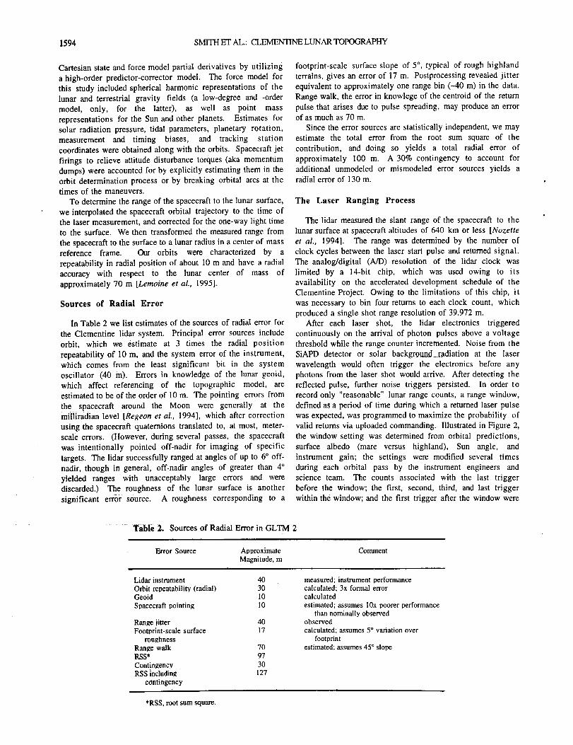
In Table 2 we list estimates of the sources of radial error for
the Clementine lidar system. Principal error sources include
orbit, which we estimate at 3 times the radial position
repeatability of 10 m, and the system error of the instrument,
which comes from the least significant bit in the system
oscillator (40 m). Errors in knowledge of the lunar geoid,
which affect referencing of the topographic model, are
estimated to be of the order of 10 m. The pointing errors from
the spacecraft around the Moon were generally at the
miiliradian level [Regeon et at., 1994], which after correction
using the spacecraft quaternions translated to, at most, meter-
scale errors. (However, during several passes, the spacecraft
was intentionally pointed off-nadir for imaging of specific
targets. The lidar successfully ranged at angles of up to 6° off-
nadir, though in general, off-nadir angles of greater than 4 °
yielded ranges with unacceptably large errors and were
discarded.) The roughness of the lunar surface is another
significant error source. A roughness corresponding to a
footprint-scale surface slope of 5 °, typical of rough highland
terrains, gives an error of 17 m. Postprocessing revealed jitter
equivalent to approximately one range bin (-40 m) in the data.
Range walk, the error in knowlege of the centroid of the return
pulse that arises due to pulse spreading, may produce an error
of as much as 70 m.
Since the error sources are statistically independent, we may
estimate the total error from the root sum square of the
contribution, and doing so yields a total radial error of
approximately 100 m. A 30% contingency to account for
additional unmodeled or mismodeled error sources yields a
radial error of 130 m.
The Laser Ranging Process
The lidar measured the slant range of the spacecraft to the
lunar surface at spacecraft altitudes of 640 km or less [Nozette
et al., 1994]. The range was determined by the number of
clock cycles between the laser start pulse and returned signal.
The analog/digital (A/D) resolution of the lidar clock was
limited by a 14-bit chip, which was used owing to its
availability on the accelerated development schedule of the
Clementine Project. Owing to the limitations of this chip, it
was necessary to bin four returns to each clock count, which
produced a single shot range resolution of 39.972 m.
After each laser shot, the lidar electronics triggered
continuously on the arrival of photon pulses above a voltage
threshold while the range counter incremented. Noise from the
SiAPD detector or solar background radiation at the laser
wavelength would often trigger the electronics before any
photons from the laser shot would arrive. After detecting the
reflected pulse, further noise triggers persisted. In order to
record only "reasonable" lunar range counts, a range window,
defined as a period of time during which a returned laser pulse
was expected, was programmed to maximize the probability of
valid returns via uploaded commanding. Illustrated in Figure 2,
the window setting was determined from orbital predictions,
surface albedo (mare versus highland), Sun angle, and
instrument gain; the settings were modified several times
during each orbital pass by the instrument engineers and
science team. The counts associated with the last trigger
before the window; the first, second, third, and last trigger
within the window; and the first trigger after the window were
Table 2. Sources of Radial Error in GLTM 2
Error Source Approximate
Magnitude, m
Comment
Lidar instrument 40Orbit repeatability (radial) 30Geoid 10Sl_acecraft pointing 10
Range iitter 40Footprint-scale surface 17
roughnessRange walk 70RSS* 97
Contingency 30RSS including 127
contingency
measured; instrument performancecalculated; 3x formal errorcalculated
estimated; assumes 10x poorer performancethan nominally observed
observedcalculated; assumes 5 ° variation over
footprintestimated; assumes 45 ° slope
*RSS, root sum square.

SMITHETAL.:CLEMENTINELUNARTOPOGRAPHY 1595
.,.o,.s,oEwi.oow
sEco.°,.s,oEWi.DOW--------a I
..ST,.=DEWI.OOW------qI r-----I.ST,.S,OEWI .OWI [--FIRST AFTER WINDOW
BEFORE_ I I NOTSAVED-w l II IIVSTART MULTIPLE I I I I
'SrART/STOPI STOPSI I I I I I I I
_ START _
RNtGE
COUNTERWINDOW
Figure 2, Clementine lidar range counter latches. The
receiver electronics was designed such that a single transmitted
laser pulse could report up to four measurements of range,
corresponding to the first three and last "hits" within the rangewindow. A range was reported when the number of photons
incident on the instrument detector exceeded the user-defined
detection threshold. "False triggers" were due to noise from
the system electronics and solar background radiation at the
laser wavelength that was received directly or reflected fromthe Moon. The range window position and width and the
threshold settings were uploaded via ground commanding and
were modified several times during each orbital pass.
latched into registers 0-5. If fewer than four triggers occurred
within the range window, the last count within the gate was
identical to the previous trigger. Initial results suggested that
later returns were increasingly likely to be due to noise, but
depending on how soon the range window opened, any of the
early returns could also be due to noise. The procedure that we
implemented to distinguish between multiple triggers for a
given transmitted pulse is discussed below.
Laser ranging was performed on orbital passes 8 to 163 in
the southern hemisphere and passes 165 to 332 in the north.
Figure 3 compares the topographic coverage obtained by
Clementine compared to that by the Apollo 15, 16, and 17
laser altimeters. Passes 8 through 19 were calibration passes,
and the data were discarded due to poor quality. During the
course of the mapping mission the lidar triggered on about
i23,000 shots, corresponding to 19% of the transmitted laser
pulses. Much of the time, the first trigger in the range window
was a true echo, but often, particularly over rough terrain, there
were multiple ("false") triggers due to noise that did not
correlate with lunar features. The main sources of noise were
the clock jitter, roughly normally distributed with -40 m
sigma; side-lobe artifacts from the laser transmitter, which are
terrain-dependent and not well understood; detector noise,
which is dependent on ambient conditions (especially
temperature variations on the SiAPD detector), range and
threshold settings, and link margin; and solar background
radiation at the laser wavelength, imparted directly on to the
detector and reflected from the lunar surface. In order to
develop a digital topographic model of the Moon, it was
necessary to develop a filter that, when applied to the data,
returned at most a single valid range value for each bounce
point. Since the detailed topography was largely unknown, it
was necessary for this filter to be based on a priori knowledge
of lunar surface properties. In the following section we
describe a stochastic model for topography, its associated
parameters, and a procedure that implemented this model as afilter.
Processing Lunar Topography
Stochastic Description of Topography
One-dimensional (l-D)topographic profiles often obey a
power law [Bell, 1975] for spectral power P, as a function of
wave number k=-l/L_ of the form
P(k) = ak-b (I)
where constants a and b are the intercept and slope on a log-
log plot. Topographic spectra are invariably "red," that is,
fall off at high wave numbers, with b ranging from I to 3
[Sayles and Thomas, 1978; Huang and Turcotte, 1989]. The
same relation applies to two-dimensional (2-D) spectra, as a
function of wave number magnitude Ikl, with b from 2 to 4
[Goff, 1990]. Planets obey a similar expression for spherical
harmonic gravity coefficients known as Kaula's rule [Kaula,
1966]. For planetary surfaces the value of b for coefficient
variances is asymptotically equal to 3 [Bills and Kobrick,
1985].
A related local scaling property of surfaces described by a
function z(x) is that they are statistically self-affine
[Mandelbrot, 1982; Goff, 1990; MaIiverno, 1991]. This
means that for any constant a > 0, there is a neighborhood
lul< of any given point x where the probability
distribution of differences z(x+au)-z(x) is the same as that
of [z(x+u)-z(x)] times a scale factor a n, where H is the
Hurst exponent [Hurst, 1951]. Viewing a small piece of terrain
at greater horizontal and vertical magnification does not
change its essential appearance. The self-affine property
implies a fractal dimension D = 3 - H, and for most power law
surfaces, D= 4-bl2 [Goff, 1990]. Planetary surfaces have
a
90 '
6o
3o
-30
-60
-60
-90
0 60 120 180 240
Longitude
300 360
Figure 3. (a) Locations of laser topographic measurementsfrom the Apollo 15, 16, and 17 laser altimeters. Co) Locations
of laser topographic measurements from the Clementine Lidar.The points shown are those remaining after filtering to remove
spurious noise hits.

1596 SMITHETAL.:CLEMENTINELUNARTOPOGRAPHY
beendescribedin termsof afractionalBrownianmodel,forwhichH ranges from 0.5 tO 0.95 [Mandelbrot, 1975, 1982].
In such models, repeated random displacements generate a self-
affine, fractal surface. Thus the mesoscale lunar highland
surface, being saturated by uncorrelated impact processes of
random size and distribution, is roughly self-affine.
At intermediate scales on the Earth, the spectral amplitudes
of long-wavelength topography are attenuated by viscous
relaxation and are smaller than predicted by a single power law
[Fox and Hayes, 1985; Gilbert and Maliverno, 1988; Goff and
Jordan, 1988]. Below some corner wave number k O, the
reciprocal of wavelength, spectral power flattens, and the
topographic variance is bounded by the square of a
characteristic height h. Such characteristic height and width
scales have been incorporated into a 2-D stochastic model for
seafloor topography [Goff and Jordan, 1988, 1989a,b], via a
stationary, random function, which is completely specified by
its covariance. The covariance, assuming a zero mean, is the
second-order moment of a topographic function z(x) :
c(u) = (z(x + u)z(x)), (2)
with the brackets indicating an average over points where the
product is defined. Goff and Jordan [1988] parameterize the
covariance in the isotropic case, for r = k 0 Iu h as
c(u) = h2Gv(r) l Gv(O), (3)
where Gv(r)=rVKv(r) and K v is the modified Bessel
function of the second kind, of Order v. For v=0.5 the
covariance takes the simple form c (u) = expf-r). The
eovariance model parameter v, which describes the scaling
behavior of topography at shorter length scales, determines
the fractal dimension D=3-v [Goffand Jordan, 1988] and
the falloff of the 2-D power spectrum,
P(k) = 4nvh2ko_[lk]2 + II-(v+_>, (4)
from which it is clear that for, large wave numbers the spectralpower falls off as Ik1-2(v+_).
Given a covariance function describing the correlation
properties of the topography, and given a set of observations
zlxi) with associated standard deviations o-i, an interpolationscheme [Tarantola and Valette, 1982] allows us to predict the
elevation at an arbitrary point x, together with confidence
limits. This procedure, also known as kriging [Matherton,
1965], generalizes the steady state Kalman filter [Kalman,
1960].
For zero-mean topographic functions, the estimate_, is
given by
Z -Iz(xj),i j
where S 0. = c(xix -xj_+Sijaio-j.. The variance of each estimateis given by
2(xl=c(0 -Z Zc(x,-xlsi,-,c(x,-x)i j
The linear system is solved by an incrementally updated
Cholesky factorization for symmetric, positive-definite
matrices [Press et al., 1986].
The interpolant _(x) is a least squares, unbiased estimate of
the elevation at any particular point, given the observations
and an a priori topographic distribution with zero mean and
covariance c(u). In order to apply it as a filter, we evaluate
the observations in sequence. An elevation z is accepted if it
lies within a confidence interval of _.(x). It is incorporated
into the topographic model, and the next interpolant is
calculated, together with its confidence interval. Such a filter
tracks the lunar surface while rejecting most of the noise.
Initial experience with multiring basins such as Orientale
found that the filter would track up to the edge of the crater rim
but would "lose lock" as the topography dropped off abruptly
and exceeded the confidence limits. A few of the noise returns
would be accepted and some of the valid hits rejected, until the
confidence limits increased and the filter found the crater floor.
Filtering in the reverse direction from the spacecraft pass
would track the floor and then miss the abrupt rise. Thus
forward and backward filtering is required.
The modified filtering algorithm proceeds as follows: each
orbital pass for which range data exist is filtered in sequence.
Elevations with respect to the dynamical ellipsoid are tested
with respect to the stochastic model to see whether they lie
within the confidence limits. If so, the elevation is flagged as
acceptable, and the model is updated. Thus, at this stage, more
than one range count may be included for each shot. Next, the
pass is filtered in reverse order, and acceptable ranges are
flagged. The union of the forward and backward pass provides
a list of ranges for this pass that make the "first cut."
The first cut incorporates a considerable amount of noise
and often deviates substantially from the "true" surface returns.
The confidence limits of the model are based on the number of
"valid" observations in the vicinity of the interpolant and are
thus narrower than in the forward or backward passes. The next
cut is formed by augmenting the confidence limits with an
added initial tolerance of 2 km. To eliminate noise while
maintaining "lock" on the planetary surface, the model is
iteratively refined by successive reduction of the added
tolerance by one half. The resulting models reject a greater
proportion of noise returns. When no further returns are
rejected, the results from the current orbital pass are added to
the filtered data set, and we proceed to the next pass.
The filtered data set grows with each succeeding pass, until
nearly all of the southern hemisphere is filtered. The second
month's mapping of the northern hemisphere overlaps in the
region from 15°S to 15°N latitude, so that the constraints from
the first month provide added stability to the filier near the
equator. The computational burden of equations (5) and _6)
grows as the cube of the number of observations, so it became
necessary to limit the model for each orbital pass to passes
within 5.6 ° of longitude. This was sufficient to include at least
two of the adjacent orbits east or west of the pass, more in the
region of overlap near the equator.
Given prior data, we adopted the values h = 8 km and found
that a correlation distance of 170 km, about 5.6 ° of latitude,
gave good results. Initial experience with orbital passes over
Orientale Basin provided estimates of the standard deviations
of first through fourth returns of 2, 5, 8, and 15 km,
respectively. These standard deviations are representative of
the unfiltered data set as a whole. Without any false returns,
electronic jitter and quantization are responsible for an
uncorrelated noise whose standard deviation is about 40 m,
while radial orbital uncertainty is of the order of 100 m

SMITH ET AL.: CLEMENTINE LUNAR TOPOGRAPHY 1597
I 0 ;, _ ,.: , ,.,
¢
s , "'",?".: . , ' :.
-lO , , ,......... ,,,.i," .... ",,,..+............... ,,'........ , ...... :.., ...... +.., ......... ,.-80 -70 -60 -50 -40 -30 -20 -10 0 10 20
Latitude
Figure 4. Results of Kalman filter of ]idar range measurements for C]ementine orbit 71. Range values thatwere accepted by the filter are noted by circled plus signs. The dark lines represent the range of acceptableelevations determined by the filter. Light lines denote the limits of acceptable ranges before adjacent passesare taken into account.
2000 Northern Highlands, 90"E-270"E, 0°N-60"N
1500
E
e-
_> 1000,
E
E
0C
Cheight=1433 m, Clength=106 km
L2
_t i, I | '
Northern Mare, 270'E-0'E, 0"N-60"N
Cheight=400 m, Clength=346 km
500 t] L2
00 500 1000
Distance, km
[Lemoine et aL, 1995]. Filtering the data yielded 72,548 validranges that were used to generate a global lunar topographic
grid and spherical harmonic model. After filtering, a few dozenranges corresponding to known impact features were manuallyincluded, and a small number of suspect ranges were excluded.Figure 4 shows an example of a filtered pass over MareOrientale and the Mendel-Rydberg Basin.
Assessment of the Stochastic Topographic Model
A convenient way to represent the covariance of surfaces is
the incremental variance y(u)= l((Az)2)[Matherton, 1965;
Davis, 1973], the variance of differences Az = z(x + u)- z(x).For stationary, random, zero-mean functions, gamma is relatedto the covariance by
7(u) = c(0)- c(u). (7)
The incremental deviation d(u)= _f-y(u) expresses the averagelocal slope of the surface and asymptotically reaches thecharacteristic height or roughness. Figure 5 shows lunar
Figure 5. Lunar incremental deviation with offset fornorthern hemisphere mare and highland regions. The mareregions are extraordinarily smooth, while farside highlandregions are much rougher and have a shorter characteristiccorrelation length. The figure plots both the sum-of-squares(L2) standard deviation and the more robust L1 deviation[Neumann and Forsyth, 1995] and parameterized fits. Fordistances of less than 100 km the deviations increase nearlylinearly, especially when robust estimates are used. Thedeviations justify our application of a self-similar model overa few degrees of scale.
1598
75°
SMITH ET AL.: CLEMENTINE LUNAR TOPOGRAPHY
50°
25°
_
_25°
_50°
_75°
75'
a) 120°E 180° 120°W 60°W 0° 60°E
50°
25°
0
_25°
_50°
_75_b) 120° 180° 240° 300° 0° 60°
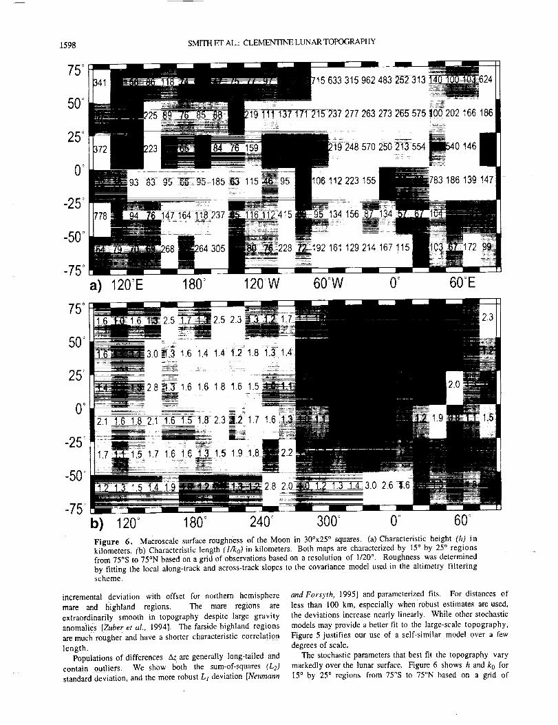
Figure 6, Macroscale surface roughness of the Moon in 30°x25 ° squares. (a) Characteristic height (h) in
kilometers. (b) Characteristic length (1/k o) in kilometers. Both maps are characterized by 15 ° by 25 ° regions
from 75°S to 75°N based on a grid of observations based on a resolution of 1/20 °. Roughness was determined
by fitting the local along-track and across-track slopes to the covariance model used in the altimetry filteringscheme.
incremenlal deviation with offset for northern hemisphere
mare and highland regions. The mare regions are
extraordinarily smooth in topography despite large gravity
anomalies [Zuber et al., 1994]. The farside highland regions
are much rougher and have a shorter characteristic correlation
length.
Populations of differences _z are generally long-tailed and
contain outliers. We show both the sum-of-squares (L2)
standard deviation, and the more robust L 1 deviation [Neumann
and Forsyth, 1995] and parameterized fits, For distances of
less than 100 km, especially when robust estimates are used,
the deviations increase nearly linearly. While other stochastic
models may provide a better fit to the large-scale topography,
Figure 5 justifies our use of a self-similar model over a few
degrees of scale.
The stochastic parameters that best fit the topography vary
markedly over the lunar surface. Figure 6 shows h and k 0 for
I5 ° by 25" regions from 75°S to 75°N based on a grid of

SMITH ET AL.: CLEMENTINE LUNAR TOPOGRAPHY 1599
00
CO
eq E
t-t_
O
Oeq_"
!
¢..O!
oO!
o
._
O0
_T _2
0., m N "__
.-_o?
e_ e_
-___
N
_._z
NNe_ _0_- N.. ©
_._ _,
K _ ._._
0 0

1600 SMITH ET AL.: CLEMENTINE LUNAR TOPOGRAPHY
Table 3. Spherical Harmonic Normalization Factors
Degree Order Factor
0 0 II 0 4(3)1 1 "_(3)2 0 "/(5)2 1 "/(5/3)2 2 (1/2)`/(513)3 0 "/(7)3 1 4(7/6)3 2 (1/2)4(7/15)3 3 (1/6)"/(7/10)4 0 "/(9)4 I _(9/10)
Factor(/,m) = _[(l-m)!(21+l)(2-5)/(l+m)!], where _5= 1
for m = 0, 8 = 0 for m _:0. From Kaula [1966].
observations based on a resolution of 1120 °. These maps will
later be interpreted in terms of macroscale roughness of the
lunar surface at length scales of 101-102 km.
Spherical Harmonic Model
The filtered data were assembled into a 0.25°x0.25 ° grid,
corresponding to the minimum spacing between orbital
passes. Figure 3b shows that most major lunar basins were
sampled by Clementine altimetry. The lidar did not return
much ranging information poleward of +78 °. Consequently,
before performing a spherical harmonic expansion of the data
set, it was necessary to interpolate over the polar regions,
corresponding to ~2% of the planet's surface area. For this
purpose, we used the method of splines with tension [Smith
and Wessel, 1990] to continue the data smoothly across the
poles. We performed a spherical harmonic expansion of the
mass=centered radii and the interpolated polar regions to yield
a global model of topography H of the form
H(A,#) = __-film(sintp)('Ctrn sin mA) (8)
L/=1 m=0
where _? and 3. are the selenocentric latitude and longitude of
the surface, Plm are the normalized associated Le_gendre
functions of degree l and azimuthal order m, Clm and Sire are
the normalized spherical harmonic coefficients with units
given in meters, and N is the maximum degree representing the
size (or resolution) of the field. Here the C and S coefficients
provide information on the distribution of global topography.
We have designated our spherical harmonic expansion of
topography, performed to degree and order 72, Goddard Lunar
Topography Model 2 (GLTM 2). The model, shown in Plate 1,
has a full wavelength spatial resolution of ~300 km. The
reliable global characterization of surface heights for the
Moon. Comparison of the data content and size of the model
to the pre-Clementine solution of Bills and Ferrari [1977] is
presented in Table 5. To first order, the shape of the Moon can
be described as a sphere with maximum positive and negative
deviations of ~8 km, both occurring on the farside (240°E,
10°S; 160°E, 75°S) in the areas of the Korolev and South Pole-
Aitken (S.P.-Aitken) basins, respectively. Departures from
sphericity are the result of the processes that shaped the Moon
(e.g., impact, volcanism, rotation, tides)early in its history
[Zuber et al., 1996]. As detailed in the next section, the
largest global-scale features are the center-of-mass/center-of-
figure (COM/COF) offset and the polar flattening, both of
which are of the order of 2 km, and the equatorial ellipticity,
which is slightly less than 1 km. However, there are
significant shorter wavelength deviations, due primarily to
impact basins, that are much larger.
Figure 7 plots the square root of the sum of the squares of
the spherical harmonic C and S coefficients for a given degree l
(8), i.e., the power per degree. This amplitude spectrum of the
topographic model has more power at longer wavelengths than
previous models owing mostly to more complete sampling of
the surface, particularly the lunar farside. The figure
demonstrates that the power of topography follows a simple
general relationship of 2 km/sphericaI harmonic degree.
Another fundamental characteristic of the lunar shape is that
the topographic signatures of the nearside and farside are very
different. As shown in Figure 8, the nearside has a gentle
topography with an rms deviation of only about 1.4 km with
respect to the best fit sphere compared to the farside, for which
the deviation is twice as large. The shapes of the histograms
of the deviations from the sphere show a peaked distribution
slightly skewed toward lower values for the nearside, while the
farside is broader but clearly shows S.P.-Aitken as an anomaly
compared to the rest of the hemisphere. The sharpness of the
nearside histogram is a result of the maria, which define an
equipotential surface (cf. Figure 15).
We have performed a comparison of elevations derived from
the Clementine lidar to control point elevations from the
Apollo laser altimeters [Davies et al., 1987]. A summary of
the Clementine and Apollo data sets is presented in Table 6.
Figure 9 indicates that where Apollo and Clementine coverage
overlaps, measured relative topographic heights generally
agree to within -200 m, with most of the difference due to our
more accurate orbit corrections [Lemoine et al., 1995] and to
variations in large-scale surface roughness (Figure 6). In
contrast, Clementine topography often differs from landmark
elevations on the lunar limb [Head et al., 1981] by as much as
several kilometers.
Differences in lunar shape parameters derived from a
comparison of Clementine and Apollo are mostly due to
Apollo's coverage being limited to north and south latitudes
26 ° and below. The greatest differences are on the farside over
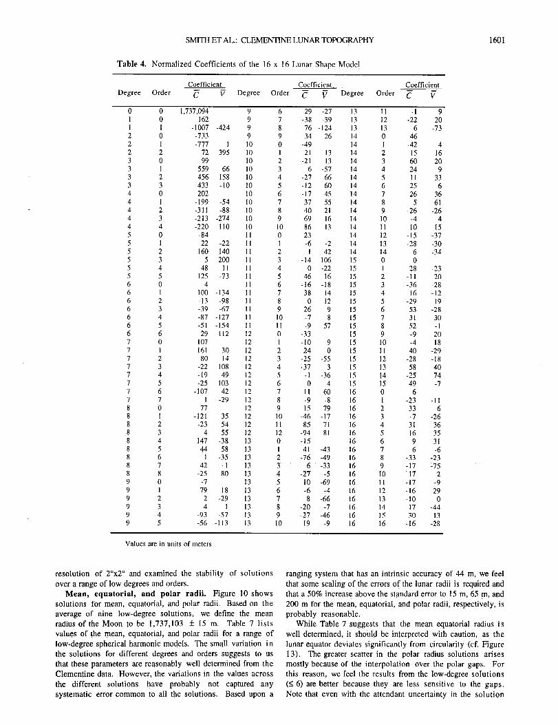
spherical horrnonic solution is normalized in the manner of a broad latitude band, much of which was not properly sampled
Kaula [1966]; normalization factors are given in Table 3.
Spherical harmonic coefficients for the first 16 degrees andorders are included in Table 4.
Topography of the Moon
Global Attributes
GLTM 2 represents a refinement of our earlier solution
GLTM 1 [Zuber et al., 1994], which represented the first
by the Apollo laser instruments.
Fundamental Parameters of the Shape
The CIementine altimetry data have made possible
improved estimates of the fundamental parameters of the
Moon's shape, which are principally derived from the long-
wavelength field. To isolate the relevant parameters, we
performed several least squares spherical harmonic expansions
of the Clementine gridded altimetric radii sampled at a
SMITH ET AL.: CLEMENTINE LUNAR TOPOGRAPHY
Table 4. Normalized Coefficients of the 16 x 16 Lunar Shape Model
Degree Order
Coefficient Coefficient Coefficient
_ _ Degree Order _ _" Degree Order _
0 0 1,737,0941 0 162
I 1 -1007 -424
2 0 -733
2 I -777 1
2 2 72 395
3 0 993 1 559 66
3 2 456 1583 3 433 -10
4 0 202
4 I -199 -54
4 2 -311 -88
4 3 -213 -274
4 4 -220 I10
5 0 -84
5 I 22 -22
5 2 160 140
5 3 5 200
5 4 48 11
5 5 125 -73
6 0 -4
6 1 100 -134
6 2 -13 -98
6 3 -39 -676 4 -87 -127
6 5 -51 -154
6 6 29 112
7 0 107
7 I 161 30
7 2 80 147 3 -22 108
7 4 -19 497 5 -25 103
7 6 -107 42
7 7 1 -29
8 0 778 1 -121 35
8 2 -23 54
8 3 4 55
8 4 147 -38
8 5 44 58
8 6 1 -35
8 7 42 -1
8 8 -25 80
9 0 -7
9 I 79 189 2 2 -29
9 3 4 -I
9 4 -93 -57
9 5 -56 -113
9 6 29 -27 13 II -I 9
9 7 -38 -39 13 12 -22 20
9 8 76 -124 13 13 -6 -73
9 9 34 26 14 0 46
10 0 -49 14 I -42 4
10 I 21 13 14 2 15 16
10 2 -21 13 14 3 60 20
10 3 6 -57 14 4 24 9
10 4 -27 66 14 5 11 33
10 5 -12 60 14 6 25 -6
10 6 -17 45 14 7 26 36
10 7 37 55 14 8 5 61
10 8 40 21 14 9 -26 -26
I0 9 69 !6 14 10 -4 4
I0 I0 86 13 14 II -10 150 23 14 12 -15 -37
1 -6 -2 14 13 -28 -30
2 I 42 14 14 6 -34
3 -14 106 15 0 0
4 0 -22 15 I -28 -23
5 46 16 15 2 -11 20
6 -t6 -18 15 3 -36 -28
7 38 14 15 4 16 -12
8 0 12 15 5 -29 19
9 26 9 15 6 53 -28
10 -7 8 15 7 31 30
I1 -9 57 15 8 52 -1
12 0 -33 15 9 -9 20
12 1 -10 9 15 10 -4 18
12 2 24 0 15 11 40 -29
12 3 -25 -55 15 12 -28 -18
12 4 -37 3 15 13 58 40
12 5 -1 -36 15 14 -25 74
12 6 0 4 15 15 49 -7
12 7 II 60 16 0 6
I2 8 -9 -8 16 1 -23 -I112 9 -15 79 16 2 33 6
12 10 -46 -17 16 3 -7 -26
12 11 85 71 16 4 31 36
12 12 -94 81 16 5 16 35
13 0 -15 16 6 9 31
13 1 41 -43 16 7 6 -6
13 2 -76 -49 16 8 -33 -23
13 3 6 -33 16 9 -17 -75
13 4 -27 -5 16 I0 17 2
13 5 10 -69 16 11 -17 -9
13 6 -6 -4 16 12 -16 29
13 7 8 -66 16 13 -10 0
13 8 -20 -7 16 14 17 -44
13 9 -27 -46 16 15 30 13
13 I0 19 -9 16 16 -16 -28
Values are in units of meters.
1601
resolution of 2°x2 ° and examined the stability of solutions
over a range of low degrees and orders.
Mean, equatorial, and polar radii. Figure 10 shows
solutions for mean, equatorial, and polar radii. Based on the
average of nine low-degree solutions, we define the mean
radius of the Moon to be 1,737,103 + 15 m. Table 7 lists
values of the mean, equatorial, and polar radii for a range of
low-degree spherical harmonic models. The small variation in
the solutions for different degrees and orders suggests to us
that these parameters are reasonably well determined from the
Clementine data. However, the variations in the values across
the different solutions have probably not captured any
systematic error common to all the solutions. Based upon a
ranging system that has an intrinsic accuracy of 44 m, we feel
that some scaling of the errors of the lunar radii is required and
that a 50% increase above the standard error to 15 m, 65 m, and
200 m for the mean, equatorial, and polar radii, respectively, is
probably reasonable.
While Table 7 suggests that the mean equatorial radius is
well determined, it should be interpreted with caution, as the
lunar equator deviates significantly from circularity (cf. Figure
13). The greater scatter in the polar radius solutions arises
mostly because of the interpolation over the polar gaps. For
this reason, we feel the results from the low-degree solutions
(< 6) are better because they are less sensitive to the gaps.
Note that even with the attendant uncertainty in the solution

1602 SMITH ET AL.: CLEMENTINE LUNAR TOPOGRAPHY
Table 5. Comparison of Global Lunar Topography Models
Parameters Bills and Ferrari [1977] GLTM 2 (This Study)
Number of observations 5631 Apollo laser 72,548 Clementine lidar12,342 orbital photo31 landmark tracking
33! 1 limb profiles21,9995°, ~150 km12x12; 1820 km-500 m (nearside only)-lkm
Total observations 72,548Spatial gridding 2°, -60 kmSpherical harmonic degree 72x72; 340 kmRegional accuracy -40 mAccuracy with respect to COM ~100 m
that the polar radii are considerably smaller than the equatorial
radii and strongly suggest an apparent flattening of about 2
km. We return to this point later.
Low-degree and -order spherical harmonic
coefficients. Table 8 summarizes solutions for low-degree
and -order spherical harmonic coefficients for a range of
topography solutions. The stability of these solutions
illustrates ctearly that the low-degree and -order shape is well
determined from Clementine altimetry.
Center-of.mass/center-of-figure offset. Figure l 1
shows solutions for the COM/COF offset. Our analysis shows
this Offset to be (-1.74, -0.75, 0.27) km in the x, y, and z
directions, respectively. It has long been known that the
Moon's geometric center was displaced from its center of mass
[Kaula et al., 1974; Sjogren and Wollenhaupt, 1976], but as a
result of the Clementine altimetry measurements, we know this
displacement deviates from the Earth-Moon line. On the
farside of the Moon the .COM/COF offset is displaced
approximately 25 ° toward the western limb ..and slightly north
of the equator [Zuber et al., 1994], in the gener_al direction of
the highlands north of S.P.-Aitken (cf. Plate 1). This
displacement, illustrated by a plot of the variation of
topography with longitude in Figure 12, is not surprising
when viewed in the context of the overall shape of the Moon
but is particularly interesting when compared, to the lunar
gravity field, which shows no such offset from the Earth-Moon
line [Lemoine et aI., 1996] (F.G. Lemoine et al., A 70th degree
and order lunar gravity model from Clementine and historical
data, submitted to Journal of Geophysical Research, 1996;
1000
i100
100 10 20 30 40 50 60 70 80
Harmonic Degree, N
Figure 7. Lunar topographic amplitude spectrum based onClementine altimetry. Note that the power of topography
follows a general relationship of 2 km per spherical harmonic
degree N.
hereinafter referred to as submitted paper). Long-wavelength
displacements that result from the irregular shape of the Moon
are thus isostatically compensated, perhaps largely by
variations in crustal thickness [Zuber et al., 1994]. Other
density variations within the interior are likely insufficient to
accomplish compensation [Neumann et al., 1996; Solomon
and Simons, 1996], though probably contribute significantly
[Solomon, 1978; Thurber and Solomon, 1978; Wieczorek and
Phillips, 1996].
Equatorial ellipticity. Another notable characteristic
of the Moon is the lack of any significant ellipticity in the
equatorial plane. Figure 13 shows the elevation with respect
to a sphere, i.e., deviations from a spheroid for all data within
1° of the equator, along with low-degree and -order spherical
harmonic terms evaluated at the equator. The (2,2) terms in the
spherical harmonic model indicate an amplitude in the
equatorial plane of about 800 m with a maximum ~40°E
longitude, smaller than the COM/COF offset, but aligned in
5
t_
O
X
4
3
Q
E52z
0-8 -4 0 4 8
EIIipsoidal Heights (km)
Figure 8. Histograms of ellipsoidal heights of all lunar
topography (solid black line), nearside topography (grey solidline), and farside topography (black dotted line).

SMITHETAL.:CLEMENTINELUNARTOPOGRAPHY
Table6. ComparisonofClementineApolloLaserandClementineLidarProfileDataSets
Parameters Apollo Clementine
Numberofobservations 7080 72,548Coverage 26S° to 26N ° 79S ° to 81N °Alon,_-track resolution 30-43 km >_20kmAcross-track resolution NA -60 km
Single shot vertical resolution 2 m 39.972 m
NA, not available•
1603
the same general direction. Figure 13 also illustrates that the
(1,1) terms are more than a factor of 2 larger than the (2,2)
terms and indicates that the largest topographic effect around
the lunar equator is the COM/COF offset. Further, the major
axis of the equatorial ellipticity (2,2 terms) is offset from the
Earth-Moon line by about 45" (E) and the (1,1) terms are also
offset about 30" (E) and presumably trying to satisfy the fact
that the maximum elevation of the highlands is not at
longitude 180°E but rather 210°E. While the major axis of the
lunar shape does not directly align toward Earth, the minimum
moment of the lunar mass does [Ferrari et al., 1980; Dickey et
al., 1994].
Triaxial ellipsoid. Because the major axis of lunar
topography is not in the Earth-Moon line, we have produced
two solutions for the best fit triaxial ellipsoid, which are
shown in Table 9. In the first (rotated) solution, we fit the
ellipsoid without constraining the direction of any of the axes.
This solution best fits all data in a least squares sense and has a
major axis that is aligned in the general direction of the
highest farside topography and with the polar axis tilted
toward Ea.rth and passing through latitude 66.0°N, longitude
8OOO
6000 " :..!"....
4000 i: "
• . : :.... -,. :. _,.._:",%:...-, : . .
E_ : •:. :.:._:. :/".i.;:-::!_:":::C,';::, :: -i. :vo= ...... ....,....._:-_._:.:..._,..::...... . -
2000 . "" ":'• "_.',t.'"._!;:'_f.,;;_!?_",.L:.':':":._.'.
-. ."'-'-"T.::..".:_:g_'_":t:,".'_" .: .'.; : ;..- - "'. !i: *;:'._';,_" _,,._ ._:_,*'_.-: .': ,.. - ." ' ,_ . ..... ,:..,..:_:.:....!.,.,_. ,.;,_:. . _..... . .. : _
,,5 • "-'" :',..?.-_';.,',_.._,¢.t:.": >. ". -::. " .-
0 _-'?:'-i"-'_z ,."L4:_.1.'r-;.'." :" " ' , --2000 . ". :" .,.:':_ ._._"d_::'_r ::,/'.' :" .- ,
• ,...:'_'...-" /_b':';'. ..... " . -
"-_,,'-_" • .". ',- ." -. "(_::'_::.' ".?: "'.: - . -
-4ooo '5',];._1., --
-6000 , , ....... . -_--
-6 -4 -2 6 _ _ _ 8Davies control points
Figure 9. Comparison of elevations from the Clementine
and Apollo laser instruments for 5141 points. Deviations
from perfect correlation include more accurate orbits
determined from Clementine tracking and macroscale
roughness of the Moon.
10.4°E. In the second (nonrotated) solution, all axes are fixed,
with the A axis along 0 ° longitude, and A and B in the
equatorial plane. This solution does not fit the Clementine
radii as well as the rotated solution and reduces the size of the
longest (A) equatorial axis, probably because the axis will be
closer to the S.P.-Aitken basin (cf. Plate 1) while increasing
the polar axis (C). Nevertheless, this model suggests a larger
equatorial mean radius than polar radius by nearly 2.5 km.
Flattening. The radii measurements have an rms
deviation about the best fit (displaced) sphere of 2.1 km with a
full dynamic range of nearly 16 km. The radius measurements
within +1 ° of the equator suggest that the mean equatorial
radius is approximately 1.2 _+ 0.2 km larger than the meanradius, while the two polar radii are about 0.8 _+ 0.5 km less
than the mean. This leads to an apparent flattening of 2.0 +0.5 km. The large uncertainty arises because the altimetry data
do not extend beyond approximately latitudes 81°N and 79°S
and extrapolation to the poles is necessary. Further, the local
topography in the polar regions is large compared to the
flattening and is inseparable from it. Another more definit!ve
1739 , , _ , , _ , _ ,
1738
E
1737.i
"Om
1736
EquatorialmimmIO_ _lI_II_,
m im
Mean
,.'_. Polar,......---'_ \ /
,, ,.,/iiiiJ
1735 _ _ ' ' ' _ _ _2x2 6x610x10 16x16
4x4 8x812x12
Degree and Order of Model
Figure 10. Low-degree and -order spherical harmonicsolutions for the Moon's mean, equatorial, and polar radii.
The stability of the solutions provides an indication of the
confidence of the estimates.
1604 SMITH ET AL.: CLEMENTINE LUNAR TOPOGRAPHY
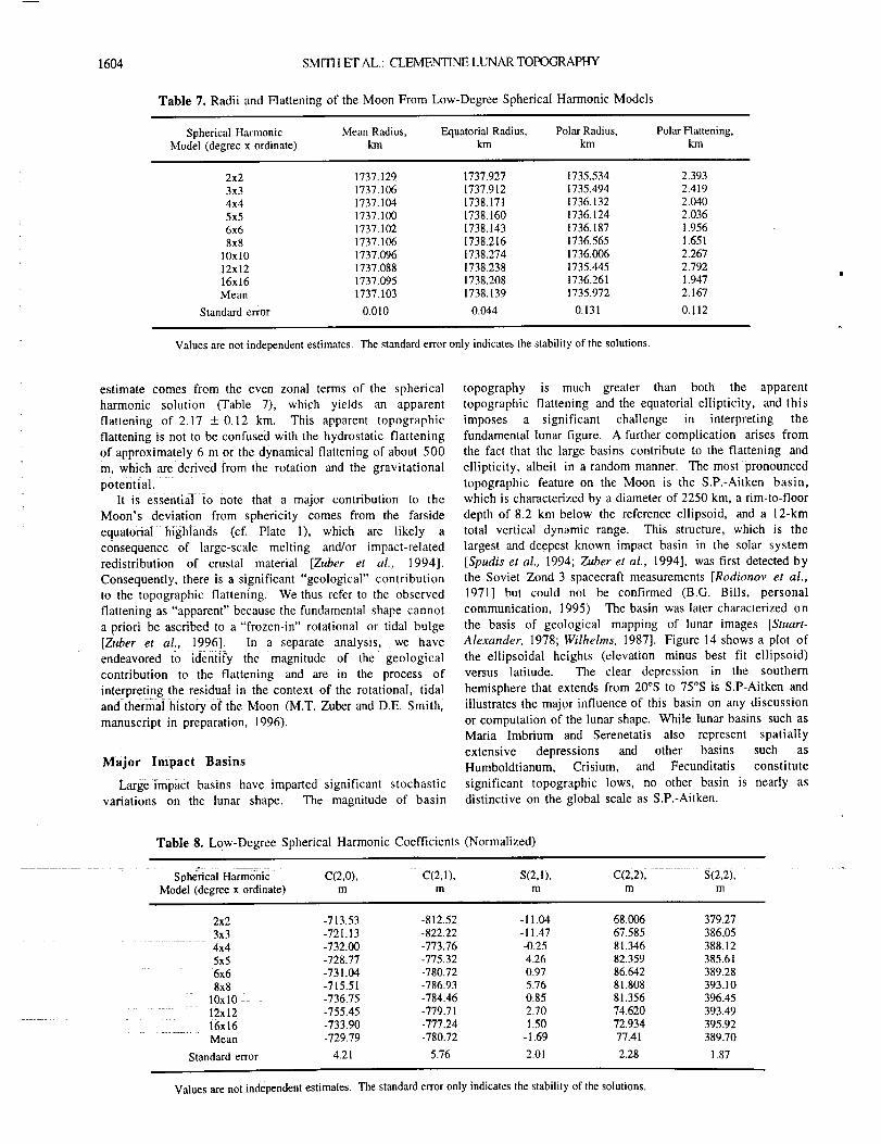
Table 7. Radii and Flattening of the Moon From Low-Degree Spherical Harmonic Models
Spherical Harmonic Mean Radius, Equatorial Radius, Polar Radius, Polar Flattening,Model (degree x ordinate) km km km km
2x2 1737.129 1737.927 1735.534 2.3933x3 1737.106 1737.912 1735.494 2.4194x4 1737.104 1738.171 1736.132 2.0405x5 1737.100 1738.160 1736.124 2.0366x6 1737.102 1738.143 1736.187 1.9568x8 1737.106 1738.216 1736.565 1.651
10xl0 1737.096 1738.274 1736.006 2.26712x12 1737.088 1738.238 1735.445 2.79216x16 1737.095 1738.208 1736.261 1.947Mean 1737.103 1738.139 1735.972 2.167
Standard error 0.010 0.044 0.131 0.!12
Values are not independent estimates. The standard error only indicates the stability of the solutions.
estimate comes from the even zonal terms of the spherical
harmonic solution (Table 7), which yields an apparent
flattening of 2.17 + 0.12 kin. This apparent topographic
flattening is not to be confused with the hydrostatic flattening
of approximately 6 m or the dynamical flattening of about 500
m, which are derived from the rotation and the gravitational
potential.
It is essential to note that a major contribution to the
Moon's deviation from sphericity comes from the farside
equatorial highlands (cf. Plate 1), which are likely a
consequence of large-scale melting and/or impact-related
redistribution of crustal material [Zuber et al., 1994].
Consequently, there is a significant "geological" contribution
to the topographic flatten{ng. We thus refer to the observed
flattening as "apparent" because the fundamental shape cannot
a priori be ascribed to a "frozen-in" rotational or tidal bulge
[Zuber et al., 1996]. In a separate analysis, we have
endeavored to ideniify the magnitude of the geological
contribution to the flattening and are in the process of
interpreting the_residual in the context of the rotational, tidal
and thermal history Of the Moon (M.T. Zuber and D.E. Smith,
manuscript in preparation, 1996).
Major Impact Basins
Large impact basins have imparted significant stochastic
variations on the lunar shape. The magnitude of basin
topography is much greater than both the apparent
topographic flattening and the equatorial ellipticity, and this
imposes a significant challenge in interpreting the
fundamental lunar figure. A further complication arises from
the fact that the large basins contribute to the flattening and
ellipticity, albeit in a random manner. The most pronounced
topographic feature on the Moon is the S.P.-Aitken basin,
which is characterized by a diameter of 2250 km, a rim-to-floor
depth of 8.2 km below the reference ellipsoid, and a 12-km
total vertical dynamic range. This structure, which is the
largest and deepest known impact basin in the solar system
[Spudis et al., 1994; Zuber et aI., 1994], was first detected by
the Soviet Zond 3 spacecraft measurements [Rodionov et al.,
1971] but could not be confirmed (B.G. Bills, personal
communication, 1995). The basin was later characterized on
the basis of geological mapping of lunar images [Stuart-
Alexander, 1978; Wilhelms, 1987]. Figure 14 shows a plot of
the ellipsoidal heights (elevation minus best fit ellipsoid)
versus latitude. The clear depression in the southern
hemisphere that extends from 20°S to 75°S is S.P-Aitken and
illustrates the major influence of this basin on any discussion
or computation of the lunar shape. While lunar basins such as
Mafia Imbrium and Serenetatis also represent spatially
extensive depressions and other basins such as
Humboldtianum, Crisium, and Fecunditatis constitute
significant topographic lows, no other basin is nearly as
distinctive on the global scale as S.P.-Aitken.
Table 8. Low-Degree Spherical Harmonic Coefficients (Normalized)
Spherical Harmonic C(2,0), C(2,1), S(2,1),
Model (degree x ordinate) m m m
c(212)_..... s(2,2_,m m
2x2 -713.53 -812.52 -11.04 68.006 379.27
3x3 -721.13 -822.22 -11.47 67.585 386.054x4 -732.00 -773.76 -0.25 81.346 388.125x5 -728.77 -775.32 4.26 82.359 385.616x6 -731.04 -780.72 0.97 86.642 389.288x8 -715.51 -786.93 5.76 81.808 393.10
10xl0 5 -736.75 -784.46 0.85 81.356 396.45i2x12 -755.45 -779.71 2.70 74.620 393A916x16 -733.90 -777.24 1.50 72.934 395.92
.......... Mean -729.79 -780.72 -1.69 77.41 389.70
Standard error 4.21 5.76 2.01 2.28 1.87
Values are not independent estimates. The standard error only indicates the stability of the solutions.

SMITHETAL.:CLEMENTINELUNARTOPOGRAPHY 1605
8OO
400
0
P -400
E -800
-1200
-1600
-2000
I I F=' I I I I I i l _--
- - _ .... AZ
Mean 267_+ 8 m
- - - _, - -zXY
Mean -748 _+_4 m
__ • • .... AXMean -1729 _+ 15 m
l i _ = J L I x I I ±Ellip 3x3 5x5 8x8 12x12
2x2 4x4 6x610x10 16x16Solution
Figure 11. Center-of-mass/center-of-figure offsets in (x,y,z)
directions for low-degree and -order spherical harmonic models
of lunar topography.
Note that Figure 14 does not show obvious evidence for a
previously proposed massive (3200 km diameter) nearside
Oceanus Procellarum basin [Wilhelms, 1987]. While support
for the existence of this basin has been offered on the basis of
Clementine altimetry [McEwen and Shoemaker, 1995],
90Radius, km Sphere
1750 r- 120 _r_..._ - 60 Radius_ I _ 1738 km
1740 _- f_ ,_'_._ j,-f"
1730 _- /__ _'_ T .... _i _ 30
o210 _#_d/ 330
240 300
270
Figure 12. Variation of lunar radii with longitude. The plot
shows that the offset between the Moon's center-of-figure and
center-of-mass deviates from the Earth-Moon line (0°-180 °longitude) and is displaced approximately 25 °, such that it is
aligned in the direction of the region of highest lunar
topography on the farside.
lacking or ambiguous evidence has been cited in other
analyses based on altimetry and crustal thickness [Spudis,
1995; Zuber et aL, 1995; Neumann et aL, 1996]. The lack of a
prominent tographic expression in association with the
hypothesized structure has been realized since the Apollo era
[Kaula et aL, 1972, 1973, 1974; Phillips et aL, 1973b; Brown
et al., ]974]. Indeed, if this basin existed, it must have either
undergone virtually complete topographic relaxation and/ or
formed prior to at least some nearside highlands which
subsequently masked the signature.
._" %2 .
E 4_ :... .:..;:...... ,_• a • • le • •
2 _ ......': "." _,_.hr--':'n,,_u... 7I. .= . :." ._. ,,_1"lW"%'==k.-JE¢'=_=l_. 1
i _ I-: ........ :'=," ...-._M'T_..-'.. E'.__-%'JIJNL_- 1• " I- 4. _'t ,"- "-" -' ""._. _q;_tCL"--. ...." "_
I,M -
-6
-8
0 60 120 180 240 300 360
Longitude, EFigure 13. All lunar radii measured by Clementine within 1° of the equator. The values are subtracted from a
mean of 1738.0 km. The dotted line shows the (1,1) term of the spherical harmonic expansion of topographyand the dashed line shows the (2,2) term. The solid line shows the sum of these terms.

1606 SMITHETAL.:CLEMENTINELUNARTOPOGRAPHY
Table9. LunarShapeandTopographicParametersFromAnalysisof ClementineAltimetry
Parameter Value,km Sigma,m
Meanradius* 1737.103 + 15Mean equatorial radius* 1738.139 :t:65Mean polar radius* 1735.972 :t:200
North polar radiust 1736.010 :t:300South polar radius? 1735.840 :k300
Best fit ellipsoid (rotated)A axis 1739.020 + 15B axis 1737.567 :1:15C axis 1734.840 + 65
Best fit ellipsoid (non-rotated)A axis 1738.056 + 17B axis 1737.843 + 17C axis 1735.485 :l: 72
* From spherical harmonic solutions (Table 7).? From spheroidal heights.
One of the puzzling characteristics of the Moon is that
nearside basins are filled with mare lavas and farside basins
tend to lack volcanic fill [WiIhelms, 1987]. The most obvious
possibility is that mare basalt on the Moon may have risen to
a hydrostatic level [Runcorn, 1974]. Inherent in this scenario
is the assumption of a common magma source depth for all
basins, filled and unfilled. If one invokes the usual
interpretation that the Moon's COM/COF offset corresponds
to a crustal thickness difference, then the nearside crust is
thinner than the farside crust. On the nearside the hydrostatic
level is located above basin floors, and it would be expected
that the elevations of maria would form a gravitational
equipotential surface. In contrast, owing to the thicker, low-
density crust, the equipotential level on the farside would be
deeper in the crust, presumably below basin floors, and magma
would not be expected to rise to an elevation that resulted in
basin flooding. Preliminary analysis of basin elevations
determined from Apollo altimetry [Sjogren and Wollenhaupt,
1976] and radar sounding [Brown et al., 1974] suggested that
nearside maria surfaces constituted an equipotential, but the
analysis was limited to equatorial basins beneath the Apollo
ground tracks. The improved spatial coverage provided by
Clementine allows a test of this hypothesis using a globally
distributed data set.
Figure 15 plots the elevations of the floors of unflooded
basins and mare surfaces of flooded basins as a function of
longitude, along with the corresponding geoid elevation (F.G.
Lemoine et al., submitted paper) at the center of each basin.
Note that maria are parallel to the geoid to within 3 km,
equivalent to 500 m on Earth when adjusting for the difference
in g. (And all but two mare basins lie within 1 kin, equivalent
to 160 m on Earth). The fact that the maria surfaces closely
parallel the geoid indicates that these surface do indeed define a
gravitational equipotential. Also note that with the exception
of S.P.-Aitken, unflooded basins tend to be at or above the
elevation of the mare surfaces. If a hydrostatic argument is
valid, these basins would not be expected to contain mare fill;
if they did, it would have been necessary for magma to have
risen above the equipotential surface. However, the floor ofS.P.-Aitken, which lies from 2 to 6 km below the mare
equipotential (and in addition, is underlain by one of the
thinnest regions of crust on the Moon [Neumann et al.,
1996]), would be expected to contain mare fill, but does not.
The Clementine data thus support a hydrostatic mechanism to
explain the absence of significant mare fill in farside basins,
except for S.P.-Aitken. For this basin it is necessary tO
invoke alternative arguments such as poor mare production
efficiency due to internal compositional or thermal
heterogeneity in this part of the early Moon [Lucey et al.,
1994].
In Figure 16 we show the relationship between eIevation
and basin age. Elevations are plotted for the floors of
unflooded basins, and the mare surfaces and floor elevations of
mare basins, the latter determined by correcting for the
thickness of mare fill. We determined fill thicknesses on the
basis of a recent analysis of depth-diameter relationships for
flooded and unflooded impact basins using Clementine
altimetry [Williams and Zuber, 1996]. The figure shows that
radial elevations of mare basins tend to correlate, at a
statistically significant level, with basin age. This
relationship could perhaps be explained if younger basins
overlapped on sites of older basins; because such areas had
been previously excavated they would have had a lower
elevation prior to later impacts. Nonmare basins do not
exhibit similar correlation, but their ages are not as well
determined as those of the mare basins. In any case, the
explanation for this observation will require more detailed
modeling and analysis than presented here. We also note that
neither mare nor unflooded basin elevations correlate with
basin diameter.
Figurebest fit
,,,, RMS = 1.9 kmJ I a , 1 l t I i i = t i I , , , , I t ] l [ i I [ [ [ t_
-60 -3() 0 30 60 90Latitude
14. Radially averaged ellipsoidal heights, corresponding to the difference between elevations and the
ellipsoid. Note the prominence of the S.P.-Aitken Basin in the southern hemisphere.

SMITHET AL.: CLEMENTINE LUNAR TOPOGRAPHY 1607
4000
E 2000
O= 0
>
m-2000
-4000
• Radius-1737 km (w/mare fill).-c--Radius-1737 km (no mare fill
--,--Geoid, 10x10 |_
. I
* - *$ -er* - - -_ ......
nearside
60
, , i , t i _ , i , , i
%?
j--- ._._ _.--"I
_._ _© O O • Q "
I
-**___**.1 +--
I
• tl
far_ide, I J , _ i ,
180
Longitude
nearside1 , , L____.L_2_t _L_Z___ _ I , ,
0 120 240 300
Figure 15. Elevations of the floors of unflooded impact basins (open circles) and mare surfaces of flooded
basins (solid circles) as a function of longitude. Also shown is the corresponding geoid elevation at the center
of each basin (solid diamonds). Note that with the exception of S.P.-Aitken, the basin floor and mare
elevations are parallel to the geoid, indicating that they define an equipotential surface.
360
Macroscale Surface Roughness
Pre-Clementine analyses of the surface roughness of the
Moon [Moore et aI., 1976] were driven by assessment of
possible manned landing sites, and consequently, focused on
much smaller length scales than are resolvable with the
Clementine aItimetry, which are best suited to analyze
wavelengths of tens to hundreds of kilometers. The Kalman
filter that we developed to remove noise from the lidar profiles
provided a framework for us to evaluate the Moon's roughness,
or local-scale topography, at these wavelengths. We
estimated the macroscale surface roughness along the
Clementine ground tracks by gridding the lidar-defived
topography data into 1/20th degree bins (approximately one
shot spacing) along each track, and fitting the local along-
track and across-track slopes to the covariance model used in
the filtering scheme [Neumann and Forsyth, 1995]. An
inherent assumption in this approach is that roughness is
1745000
1740000
Ev
=1735000,m
"0
re
Korolev
Hertzsprung MendeI-Rydberg• ......... ./' Tranquillitatis
Men_e'e_l _ i!Fecunditatis
Orientale e"L _. . . Aitken
1730000 Imb-rlum __ Coulomb-Sarton
Freu ndlich-Sharonov
1725000 ___________1.... t..... t .... i,,,, i =, _±____t___ .....3.75 3.8 3.85 3.9 3.95 4 4.05 4.1
Age (BY)
Figure 16. Correlation of basin elevation with age. Results are shown for basins with (solid squares) andwithout (solid circles) mare fill. Results show a correlation of elevation with age for mare basins. This result
persists after correction in which the mare fill is removed (open squares) using the method of Williams and
Zuber [1996]. Basins without mare fill do not show any correlation with elevation.
4.15

1608
al
SMITH ET AL.: CLEMENTINE LUNAR TOPOGRAPHY
b)
Figure 17. Three-d{mensional relief maps of (a) the nearside western hemisphere and (b) the farside S.P.-
Aitken basin. The figure illustrates the flatness of lunar maria as compared to the highlands. In Figure 17a the
Orientale Cordillera appears at the bottom left with depressions associated with Gfimaldi and Cruger along its
margin, while Humorum Basin can be seen at the bottom center. The Montes Ural (upper center), AristarchusPlateau (center), and Montes Carpatus (lower fight) rise above the mafia. Craters Lichtenberg, Seleucus,
Marius, Aristarchus, and Copernicus, from left to right, are resolved as 1- to 2-km-deep depressions.
Ptolemaus appears at the lower right. In Figure 17b the S.P.-Aitken basin covers the central bottom of the
figure. For both maps the vertical exaggeration is 60:1.
locally isotropic. The roughness consists of an estimate of
the characteristic height, or overall variance, of the sample as
a whole, together with an estimate of the distance over which
local deviations are expected to attain 80% of this value.
We produced a macroscale roughness map of the Moon in
30°x25 ° squares (Figure 6), which shows the marked regional
variability of the best fitting height parameter for
topography. A robust measure of incremental variance (h) or
median roughness, varies from less than 0.5 km over the
northern nearside mafia to more than 2 km over the highland
regions. The roughness strongly affects the comparability of
lidar measurements from different spacecraft ground tracks, and

SMITHETAL.:CLEMENTINELUNARTOPOGRAPHY 1609
5000
E
o
a)
g
Z_
-5000
0
Figure 18.
iooo ..... 2600 30ooRoughness, m
Correlation of lunar surface roughness and
elevation. The straight line is a best fit linear regression
significant at the 99% level.
accounts for much of the difference between Apollo-era
measurements and the Clementine altimetry (Figure 9),
As previously noted from the Apollo altimetry [KauIa et al.,
1972], Clementine topography shows the lava-flooded mare
basins to be extremely level, with typical slopes less than 1
part in 103 . Figure 17a is a 3-D relief map of the nearside
western hemisphere, which illustrates the flatness of the
northern maria. Over a region of nearly 2400 km 2, the median
absolute deviation of the maria from a smooth (quadratic)
surface is only 200 m. Par.ticularly smooth are the northwest
Oceanus Procellarum and the lmbrium Basin. Figure t7b
illustrates the considerably greater relief of farside highlands
in the vicinity of the S.P.-Aitken basin. For comparison, the
deviation of this region from a quadratic surface is 2400 m.
As an indicator of the scale of surface processes, the
roughness of the Moon appears to reflect more than simply the
presence or absence of maria. For example, the S.P.-Aitken
basin (180°E, 50°S), an albeit anomalous feature, is
topographically smoother than the surrounding highland
regions. Factors that correlate with roughness are elevation
and age. Figure 18 indicates that the positive correlation
between elevation and roughness displays a quasi-linear
relationsip and is statistically significant at the 99% level,
Elevated areas on Earth and Venus also tend to exhibit steeper
slopes and greater roughness at generally comparable length
scales [Sharpton and Head, 1986; Ford o_nd Pettengill, 1992;
Harding et at., 1994; Garvin and Frawley, 1995], though the
processes that produced the roughness are distinctive on the
various planets.
Summary
Topographic measurements from the Clementine lidar have
been used to produce an accurate model for the shape of the
Moon. We have analyzed in detail the data and model, with
emphasis on spatial resolution, spectral content, and error
sources, and have obtained refined estimates of the
fundamental parameters of the lunar shape. The largest global-
scale features are the center-of-mass/center-of-figure offset and
the apparent polar flattening, both of the order of 2 kin. In
comparison, the equatorial ellipticity, at 800 m, is small.
Redistribution of crustal material from major impacts has
significantly modified the lunar shape, with the magnitude of
major impact basin topography exceeding the magnitudes of
Moon's long wavelength deviations from sphericity. Mare
basin elevations parallel the geoid and thus define a
gravitational equipotential surface, while the floors of
unflooded large basins, except for S.P.-Aitken, lie above the
equipotential. Mare and unflooded basin elevations are
consistent with a hydrostatic mechanism for the absence of
significant farside maria except for S.P.-Aitken. The observed
absence of significant mare deposits in this structure implies
major compositional and/or thermal heterogeneity in the lunar
interior
A comparison of elevations derived from the Clementine
lidar to control point elevations from the Apollo laser
altimeters indicates that measured relative topographic heights
generally agree to within -200 m on the maria. Deviations
from a quadratic surface increase to over 2 km on the farside
highlands. The observed scatter of the observations is due to
noncoincidence of measurements and the roughnes_ of
macroscale (10L102 kin) topography. Lunar surface roughness
at these length scales correlates with surface elevation and age.
The improved knowledge of topography provided by
Clementine has implications for lunar structure and evolution.
Models of internal structure that require both high-quality
topography and gravity measurements will continue to be
hampered, at least in the near term, by the lack of farside
gravity observations, which require direct Doppler tracking of
an orbiting spacecraft. However, both the topography and
gravity (F.G. Lemoine et al., submitted paper) data sets are
sufficiently improved from pre-Clementine versions to enable
many global: and regional-scale problems to be addressed. Of
particular value would be the isolation of effects of major
impa.cts, heterogeneous crustal production, and orbital and
tidal influence on the long-wavelength shape, in order to
understand the contributions of these fundamental processes in
the formative development of the Moon.
Acknowledgments. We are grateful to P. Rustan and the BallisticMissile Defense Organization for implementation of the mission; I.Lewis for providing significant insight concerning the function and
operation of the lidar instrument; G. Elman, S. Fricke, E. Pavlis, and A.Brenner for assistance in the data reduction; D. Rowlands for support inthe orbit and spacecraft pointing corrections; H.-S. Park for providingthe Clementine lidar ground calibration data; H. Taylor for reformatting
the raw range data; R Reisse and C. Acton for information onspacecraft timing errors; J. Garvin for discussions about lunar surfaceroughness; M. Davies for making available the lunar control networkcoordinates; and K Williams for providing basin depths and mafiathicknesses. In addition, we thank W. Sjogren for helpful comments andR. Phillips for a detailed review that greatly improved the paper. This
work was supported by grants from the NASA/Ballistic Missile DefenseOrganization C!ementin_ Project, the NASA Planetary Geology andGeophysics Program, and the NASA Lunar and Asteroid Data AnalysisProgram. Altimetry processing algorithms were developed in support Ofthe Mars Observer and Mars Global Surveyor laser altimetryinvestigations. The lidar profiles, global grid, and spherical harmonic
model are archived in the Geophysics Node of the NASA PlanetaryData System at Washington Uni,_ersity, St. Louis, Missouri.
References
Arthur, D. W. G., and P. Bates, The Tucson selenodetic triangulation,Commun. Luna Planet. Lab., 7, 313-361, 1968.
Baldwin, R. B., The Face of the Moon, p. 239, Univ. of Chicago Press,Chicago, II1., 1949.

1610 SMITH ET AL.: CLEMENTINE LUNAR TOPOGRAPHY
Baldwin, R. B., The Measure of the Moon, p. 488, Univ. of Chicago
Press, Chicago, I11., 1963.
Bell, T. H., Statistical features of sea-floor topography, Deep Sea Res.,
22, 883-892, 1975.
Bills, B. G., and A. J. Ferrari, A harmonic analysis of lunar topography,
Icarus, 31, 244-259, 1977.
Bills, B. G., and M. Kobrick, Venus topography: A harmonic analysis, J.
Geophys. Res., 90, 827-836, 1985.Brown, W, E. J., et al., Elevation profiles of the Moon, Proc. Lunar Sci.
Conf., 5th, 3037-3048, 1974.Davies, M. E., T. R. Colvin, and D. L. Meyer, A unified lunar control
network: The nearside, Z Geophys. Res., 92, 177-184, 1987.
Davis, J. C., Statistics and Data Analysis in Geology, John Wiley, New
York, 1973.
Dickey, J. O., et al., Lunar laser ranging: A continuing legacy of the
Apollo program, Science, 265, 482-490, 1994.Duxbury, T., et al., Pre-launch models of the Clementine spacecraft and
remote sensing science instruments for geodesy, cartography and
dynamical sciences, BMDO DSPE Internal Report, January 1994.
Ferrari, A. J., W. S. Sinclair, W. L. Sjogren, J. G. Williams, and C. F.
Yoder, Geophysical parameters of the Earth-Moon system, J.
Geophys. Res., 85, 3939-3951, 1980.Ford, P. G., and G. H. Pettengill, Venus topography and kilometer-scale
slopes, J. Geophys. Res., 97, 13,103-13,114, 1992.Fox, C. G., and D. E. Hayes, Quantitative methods for analyzing the
roughness of the seafloor, Rev. Geophys., 23, 1-48, 1985.
Garvin, J. B., and J. J. Frawley, Topographic ruggedness properties of
Venus and Earth, Geoscientist, 5, 13-16, 1995.Gilbert, L, E., and A. Malivemo, A characterization of the spectral
density of residual ocean floor topography, Geophys. Res. Lett., 15,
1401-1404, 1988.
Goff, J. A., Stochastic modeling of seafloor topography, Ph.D.
dissertation, Mass. Inst. of Technol., Cambridge, 1990.
Goff, J. A., and T. H. Jordan, Stochastic modeling of seafloor
morphology: Inversion of Sea Beam data for second-order statistics,
J. Geophys. Res., 93, 13,589-13,608, 1988.Goff, J. A., and T. H. Jordan, Stochastic modeling of seafloor
morpholgy: Resolution of topographic parameters by Sea Beam data,
IEEE J. Oceanic Eng., 14, 326-337, 1989a.Goff, J. A., and T. H. Jordan, Stochastic modeling of seafloor
morphology: A parameterized Ganssian model, Geophys. Res. Lett.,
16, 45-48, 1989b.
Harding, D. J., J. L. Burton, and J. J. Frawley, Satellite laser altimetry of
terrestrial topography: Vertical accuracy as a function of surface
slope, roughness, and cloud cover, IEEE Trans. Geosci. Remote
Sens., 32, 329-339, 1994.Head, J. W., E. Robinson and R. J. Phillips, Topography of the Orientale
basin, Lunar Planet. Sci. Conf., XII, 421-423, 1981.
Hopmann, J., GeneraI-Katalog absoluter Hohen auf dem Kond, Ann.Univ. Sternw. Wien, 26, 7, 1967.
Huang, L, and D. L. Turcotte, Fractal mapping of digitized images:
Application to the topography of Arizona and comparison to
synthetic images, J. Geophys, Res., 94, 7491-7495, 1989.
Hurst, H. E., Long-term storage capacity of reservoirs, Trans. Am. Soc.
Civ. Eng., 116, 770-808, 1951.Jones, R. L., Estimates of the Moon's geometry using lunar orbiter
from Clementine and historical S-band data, in Global Gravity Field
and Its Temporal Variations, edited by R. Rapp, A. Cazenave, and R.
Nerem, Springer-Verlag, New York, 1996.Lucey, P. G., P. D. Spudis, M. Zuber, D. Smith, and E. Malaret,
Topographic-compositional units on the Moon and the early evolution
of the lunar crust, Science, 266, 1855-1858, 1994.
Malivemo, A., Inverse square-root dependence of mid-ocean-ridge
flank roughness on spreading rate, Nature, 352, 58-60, 1991.
Mandelbrot, B., Stochastic models for the Earth's relief, the shape andthe fractal dimensions of the coastlines, and the number-area rule for
islands, Proc. NatL Acad Sci., 72, 3825-3828, 1975.
Mandelbrot, B., The Fractal Geometry of Nature, p. 468, W. H.
Freeman, New York, 1982.
Matherton, G., Les Variables Regionalisees et Leur Estimation, Une
Application de la Theorie des Fonctions Aleatoires aux Sciences de la
Nature, p. 306, Masson, Paris, 1965.
McCarthy, J. J., S. Rowton, D. Moore, S. Luthcke, D. E. Pavlis, L. S.Tsaoussi, D. D. Rowlands, and J. A. Marshall, GEODYN systems
descriptions and operations manuals, Contractor Rep., NASA
Goddard Space Flight Cent. and Hughes/STX, Greenbelt, Md., 1994.
McEwen, A. S., and E. M. Shoemaker, Two classes of impact basins onthe Moon (abstract), Lunar Planet. Sci. Conf., XXVI, 935-936, 1995.
Mills, G. A., and P. V. Sudbury, Absolute coordinates of lunar features,
Icarus, 9, 538-561, 1968.
Moore, H. J., G. L. Tyler, J. M. Boyce, R. W. Shorthill, T. W. Thompson,
D. E. Wilhelms, and S. S. C. Wu, Correlation of photogeology and
remote sensing data along Apollo 14, 15 and 16 bistatic radar ground
tracks, U.S. Geol. Survey Open File Report, 76-298, 101 pp., April1976.
Neumann, G. A., and D. W. Forsyth, High resolution statistical
estimation of seafloor morphology: Oblique and orthogonal fabric on
the mid-Atlantic ridge, Mar. Geophys. Res., 17, 221-250, 1995.
Neumann, G. A., M. T. Zuber, D. E. Smith, and F. G. Lemoine, The
lunar crust: Global signature and structure of major basins, J.
Geophys. Res., 101, 16,841-16,863, 1996.
Nozette, S., et al., The Clementine mission to the Moon: Scientific
overview, Science, 266, 1835-1839, 1994.
Phillips, R. J., et al., Apollo lunar sounder experiment, in Apollo 17Preliminary Science Report, pp. 1-26, NASA, Greenbelt, Md.,
1973a.
Phillips, R. J., et al., The Apollo 17 Lunar Sounder, Proc. Lunar Planet.
Sci. Conf., 4th, 2821-2831, 1973b.Press, W. J., B. P. Flannery, S, A. Teukolsky, and W. T. Vetterling,
Numerical Recipes, p. 818, Cambridge Univ. Press, New York, 1986.
Putney, B. H., General Theory for Dynamic Satellite Geodesy, in The
National Geodetic Satellite Program, NASA Spec. Publ., SP-365,
1977.
Regeon, P. A., R. J. Chapman and R. Baugh, Clementine: The DeepSpace Program science experiment, Rep. IAA-L-0501, pp. 1-13, Int.
Acad. of Astron., 1994.
Roberson, F. I., and W. M. Kaula, Apollo 15 laser altimeter, Apollo 15
Preliminary Science Report, NASA Spec. PubL, SP-289, 25, 48-50,1972.
Rodionov, B. N., et al., New data on the Moon's figure and relief based
on results from the reduction of Zond-6 photographs, Cosmic Res., 9,
imagery and Apollo laser altimeter data, NASA Tech. Rep., TR R-407, 410-417, 1971.1973. Runcoru, S. K., On the origin of mascons and moonquakes, Proc. Lunar
Kalman, R. E., A new approach to linear filtering and prediction Planet, Sci. Conf., 5th, 3115-3126, 1974.
problems, Trans. ASMEJ. Basic Eng. Ser. D, 83, 35-46, 1960. Runcoru, S. K., and B. M. Gray, The figure of the Moon, in Mantles ofKaula, W. M., Theory of Satellite Geodesy, p. 124, Blaisdell, Waltham, the Terrestrial Planets, pp. 165-173, John Wiley, New York, 1967.
Mass., 1966. = Runcom, S. K., and S. Hofmann, The shape of the Moon, in The Moon,Kaula, W. M., G. Schubert, R. E. Lingenfelter, W. L. Sjogren, and W.R. edited by S. K. Runcorn and H. C. Urey, pp. 22-31, D. Reidel,
Wollenhaupt, Analysis and interpretation of lunar laser altimetry, Norwell, Mass., 1972.
Proc. Lunar sci. Conf., 3rd, 2189-2204, 1972. Runcorn, S. K., and M. H. Shrubsall, The figure of the Moon, Phys.
Kaula, W. M., G. Schubert, R. E. Lingenfelter, W. L. Sjogren, and W.R. Earth Planet. Inter., 1, 317-325, 1968.
Wollenhaupt, Lunar topography from Apollo 15 and--i_; t_iser Runeorn, S. K., and M. H. Shrubsall, The figure of the Moon, Phys.
altimetry, Proc. Lunar Sci, Conf, 4th, 2811-2819, 1973. Earth Planet. Inter., 1, 317-325, 1970.
Kaula, W. M.I"G. Schubert, R. E. Lingenfelter, W. L. Sjogren, and W.R. Sayles, R. S., and T. R. Thomas, Surface topography as a nonstationary
Wollenhaupt, Apollo laser altimetry and inferences as to lunar _ random process, Nature, 271, 431-434, 1978.
surface structure, Proc. Lunar Planet. Sci. Conf., 5th, 3049-3058, Sharpton, V. L., and J. W. Head, A comparison of the regional slope
1974. characteristics of Venus and Earth: Implications for geologic
Lemoine, F. G., D. E. Smith, M. T. Zuber, D. D. Rowlands, and G.A. processes on Venus, Z Geophys. Res., 91, 7545-7554, 1986.
Neumann, Results from the Clementine lunar geodesy investigation, Sjogren, W. L., and W. R. Wollenhaupt, Lunar shape via the Apollo
Astrodynamics, 90, 201-223, 1995. laser altimeter, Science, 179, 275-278, 1973.
Lemoine, F. G., D. E. Smith, M. T. Zuber, and G. A. Neumann, High Sjogren, W. L., and W. R. Wollenhaupt, Lunar global figure from mare
degree and order spherical harmonic gravity modeling of the Moon surface elevations, Moon, 15, 143-154, 1976.

SMITHETAL.:CLEMENTINE LUNAR TOPOGRAPHY 1611
Smith, W. H. F., and P. Wessel, Gridding with continuous curvature
splines in tension, Geophysics, 55, 293-305, 1990.
Solomon, S. C., The nature ofisostasy on the Moon: How big a Pratt-fall
for Airy models?, Proc. Lunar Planet. ScL Conf, 9th, 3499-3511,1978.
Solomon, S. C., and M. Simons, The isostatic state of the lunar highlands
from spatio-spectral localization of gravity, topography and surface
chemistry (abstract), Lunar Planet. Sci. Cot*f, XXVII, 1245-1246,1996.
Spodis, P. D., Clementine laser altimetry and multi-ring basins on the
Moon (abstract), Lunar Planet. Sci. Conf., XXVI, 1337-1338, 1995.
Spudis, P. D., R. A. Riesse, and J. G. Gillis, Ancient multiring basins on
the Moon reveaIed by Clementine laser altimetry, Science, 266,
1848-1851, 1994.
Stuart-Alexander, D. E., Geologic map of the central farside of the
Moon, U.S. Geol. Surv. Map, 1-1047, 1978.
Tarantola, A. and B. Valette, Generalized nonlinear inverse problems
solved using the least squares criterion, Rev. Geophys., 20, 219-232,1982.
Thurber, C. H., and S. C. Solomon, An assessment of crustal thickness
variations on the lunar near side: Models, uncertainties, and
implications for crustal differentiation, Proc. Lunar Planet. Sci. Conf,9th, 3481-3497, 1978.
Watts, C. B., The marginal zone of the Moon, Astrott Pap. Amr.
Ephemeris Naut. Almanac, 17, 1963.
Wieczorek, M. A., and R. J. Phillips, The structure and compensation of
the lunar highland crust (abstract), Lunar Planet. Sci. Conf., XXVII,1431-1432, 1996.
Wilhelms, D. E., The Geologic History of the Moon, 302 pp., U.S. Govt.
Print. Off., Washington, D.C., 1987.Williams, K. K., and M. T. Zuber, Re-evaluation of mare thicknesses
based on lunar crater depth-diameter relationships (abstract), Lunar
Planet. Sci. Conf., XXVII, 1441-1442, 1996.
Wollenhaupt, W. R., and W. L. Sjogren, Apollo 16 Laser Altimeter, in
Apollo 16 Preliminary Science Report, NASA Spec. Publ., SP-315,30: 1-5, 1972.
Wollenhaupt, W. R., R. K. Osburn, and G. A. Ransford, Comments on
the figure of the Moon from landmark tracking, Moon, 5, 149-157,
1972.
WollenhaupL W. R., W. L. Sjogren, R. E. Lingenfelter, G. Schubert, and
W. M. Kaula, Apollo 17 laser altimeter, in Apollo 17 Preliminary
Science Report, NASA Spe¢. Publ., SP-315, 33, 41-43, 1974.
Zisk, S. H., A new, Earth-based radar technique for the the
measurement of lunar topography, in Conference on Lunar
Geophysics, pp. 296-306, Lunar Planet. Inst., Houston, "rex., 1971.
Zisk, S. H., A new, Earth-based radar technique for the measuremem of
lunar topography, Moon, 4, 296-306, 1972.Zuber, M. T., D. E. Smith, F. G. Lemoine, and G. A. Neumann, The
shape and internal structure of the Moon from the Clementine
mission, Science, 266, 1839-1843, 1994.
Zuber, M. T., D. E. Smith, G. A. Neumann, and F, G. Lemoine, Gravity,
topography and the geophysics of the Moon from the Clementine
mission (abstract), Lunar Planet. Sci. Conf., XXVI, 1581-1582, 1995.
Zuher, M. T., D. E. Smith, G. A. Neumann, and F. G. Lemoine, What
factors control the long wavelength shape of the Moon? (abstract),
Lunar Planet. Sci. Conf., XXVII, 1511-1512, 1996.
F.G. Lemoine, Space Geodesy Branch, Code 926, NASAJGoddard
Space Flight Center, Greenbelt, MD 20771.
(lemoine @olympus.gsfc.nasa.gov)G.A. Neumann, Department of Earth and Planetary Sciences, Johns
Hopkins University, Baltimore, MD 21218.
(neumann @utopia.eps.jhu.edu)D.E. Smith, Laboratory for Terrestrial Physics, Code 920,
NASA/Goddard Space Flight Center, Greenbelt, MD 20771.
(dsmith @tharsis.gsfc.nasa.gov)
M.T. Zuber, Department of Earth, Atmospheric and Planetary
Sciences, Massachusetts Institute of Technology, Cambridge, MA
02139-4307. ([email protected])
(Received June 24, 1996; revised September 16, 1996;
accepted September 18, 1996.)
