topography associated with crustal flow in continental...

Geophys. J. Int. (2008) doi: 10.1111/j.1365-246X.2008.03890.x

GJI

Tec

toni

csan

dge

ody

nam

ics

Topography associated with crustal flow in continental collisions,with application to Tibet

R. Bendick,1 D. McKenzie2 and J. Etienne3

1Department of Geology, University of Montana, 32 Campus Dr., Missoula, MT 59812-1296, USA. E-mail [email protected] Laboratories, University of Cambridge, Madingley Road, Cambridge, CB3 0EZ, UK3Laboratoire de Spectrometrie Physique, Universite J. Fourier CNRS, 140 av. de la Physique, Saint-Martin-d’Heres, France

Accepted 2008 June 13. Received 2008 June 13; in original form 2007 October 1

S U M M A R YCollision between an undeformable indenter and a viscous region generates isostaticallycompensated topography by solid-state flow. We model this process numerically, using afinite element scheme. The slope, amplitude and symmetry of the topographic signal dependon the indenter size and the Argand number of the viscous region, a dimensionless ratio ofgravitational body forces to viscous forces. When applied to convergent continental settings,these scaling rules provide estimates of the position of an indenter at depth and the mechanicalproperties of the viscous region, especially effective viscosity. In Tibet, forward modellingsuggests that some elevated, low relief topography within the northern plateau may be attributedto lower crustal flow, stimulated by a crustal indenter, possibly Indian lithosphere. The best-fitmodel constrains the northernmost limit of this indenter to 33.7◦N and the maximum effectiveviscosity of Eurasian middle and lower crust to 1 × 1020 ± 0.3 × 1020 Pa s.

Key words: Numerical solutions; Continental tectonics: compressional; Dynamics of litho-sphere and mantle; Asia.

1 I N T RO D U C T I O N

Persistent topography on Earth is the sum of signals from a varietyof tectonic and erosional processes, expressed over a wide rangeof spatial scales. The length scale of these signals can be usedto decipher their likely cause. For example, high-amplitude, short-wavelength topography must be supported by stresses in the strongupper crust, with the topography itself being generated by tectonicsand erosion. Such elastic flexure supports features with character-istic wavelengths, dependant on flexural rigidity; folding and brittlefaulting produce surface displacements, with scaling characteristicsthat also depend on crustal rheology. The thickness of the elasticlayer can also be estimated from the vertical distribution of seis-mic moment release in the continental crust (Maggi et al. 2000;Jackson et al. 2004), correlations between gravity and topographicloads (Burov & Diament 1995; McKenzie 2003), continental heatflow (McKenzie et al. 2005), seismic wave velocity (e.g. Shapiro& Ritzwoller 2002) and rock mechanics (Brace & Kohlstedt 1980).Beneath Tibet, we assume that the part of the crust that behavesas a viscous fluid is everywhere overlain by a thin lid of elasticuppermost crust. The observed relationship between gravity and to-pography (Braitenberg et al. 2003) and flexural modelling (Maseket al. 1994) require this elastic lid to have a thickness of less than10 km beneath the Qiangtang terrain. Therefore, at the wavelengthswith which we are concerned, of between 100 and 500 km, theelastic layer has little effect on the vertical motions. It is, how-ever, sufficiently strong to impose a constant horizontal velocity atthe upper surface. In contrast, the longest wavelength topographic

signals, such as the entire Tibetan Plateau, cannot be produced bydeformation of the crust alone but must instead be the result of thedeformation of the entire lithosphere (Houseman & England 1986;Royden 1996; Tapponnier et al. 2001; Vanderhaeghe et al. 2003;Thatcher 2006; Meade 2007).

Our concern, here, is with the intermediate scale contributions tosurface topography from deeper parts of the crust, which are stillpoorly understood. Where the total crustal thickness is large, thedeep parts of the crust are likely to deform as a viscous fluid (Royden1996; Clark & Royden 2000; McKenzie & Jackson 2002; Beaumontet al. 2004). This deformation has the potential to generate persistentintermediate-wavelength topography that can be used to constrainthe viscosity of the middle and lower crust.

We develop a 2-D continuum fluid model of the crustal be-haviour in a continental collision, to test one mechanism for buildingintermediate-wavelength topography. The model is designed to in-corporate three critical features: convergence, lateral rheologicalheterogeneity and rigid, deformable boundary conditions. Thesefeatures are guided by independent geological and geophysical ob-servations of the middle and lower crust in active tectonic settings.We model convergent conditions because continental shortening of-ten produces a thick, mostly aseismic lower crust (e.g. Jackson et al.2004), which is likely to undergo continuous deformation. We modellateral rheological heterogeneity because continental collision jux-taposes bodies of crustal material with differing temperatures andmechanical properties. Finally, we use boundary conditions that al-low the upper surface of the crust and the Moho to change shape(Flesch et al. 2005; Bendick & Flesch 2007).

C© 2008 The Authors 1Journal compilation C© 2008 RAS

2 R. Bendick, D. McKenzie and J. Etienne

Figure 1. (a) Initial geometry for the numerical problem. The boundary conditions on labelled boundaries are discussed in the text. The heavy line outlinesthe region that is rigid and undeformable. (b) Deformed mesh at t ′ = 50. The mesh varies in density to accommodate regions of high strain. �2 and �6 arenow deformed, as mesh nodes are advected during each iteration. Solutions for velocity and pressure are calculated at each iteration, for the entire region �.

Throughout this paper, ‘rigid’ is used to denote a boundary wherethe boundary-parallel velocity is specified, ‘free’ is one wherethe boundary-parallel stress is zero, ‘undeformable’ denotes onewhere boundary-normal velocity is specified to be zero and ‘de-formable’ one where the boundary-normal stress is specified. Rigid,deformable boundary conditions, therefore, constrain parallel ve-locities and normal stresses on the boundaries of viscous regionsin the crust. We use these boundary conditions to model the upperboundary of the crust because we are concerned with wavelengthsthat are large enough to be unaffected by flexural support. We believethat these conditions are appropriate for modelling the behaviourof Tibet, as India and Asia converge. Rigid, deformable boundaryconditions permit crustal thickness changes to occur because theboundary conditions are on the vertical stress, and therefore, theboundaries are free to move vertically.

We consider a model in which a rigid sheet of thickness a isdriven into a viscous layer of thickness h at a constant velocity U 0

(Fig. 1a). Where the upstream flow is unaffected by the motion ofthe rigid sheet, the velocity of the crust does not vary with depth,and the surface is horizontal. As the edge of the sheet passes belowa point on the surface, the surface moves first up and then down,before again becoming horizontal far downstream from the edgeof the sheet, where the velocity again becomes horizontal but nowvaries linearly with depth.

McKenzie et al. (2000) modelled the time-dependent behaviourof a viscous layer of viscosity η1 and density ρ 1 overlying a half-space of viscosity η2 and density ρ 2(>ρ 1), when the intial heightsof the upper and lower boundaries of the layer, ξ and ζ , are givenby ξ 0 sin kx and ζ 0 sin kx , where k = 2π/λ is the wavenumber ofthe disturbance and λ is its wavelength. This system has two timeconstants. When ξ 0 = ζ 0 and kh � 1, isostatic compensation oc-

curs with a time constant τ b. The other mode is excited when ξ 0 =−ζ 0, corresponding to variations in crustal thickness. These decayon a timescale of τ a, due to lateral flow within the crust. When theviscosity of the half-space is much greater than that of the layerand the wavelength of the disturbance is large compared with thelayer thickness, McKenzie et al. (2000) showed that τ a � τ b. Adifferent form of behaviour occurs when kh � 1. Though thereare still two time constants, they are associated with the relaxationof disturbances to the top and bottom surfaces of the layer. Thetime constants are only affected by the properties of the materialon either side of the boundary concerned and are independent ofthe thickness of the layer. We are principally concerned with thetopography of the upper surface of the layer and with wavelengthsλ < 6h. McKenzie et al.’s calculations show that the time-dependentbehaviour of the upper and lower surfaces are then essentially inde-pendent, and that the surface topography is scarcely affected by theboundary conditions imposed at the base of the layer.

We are concerned with the vertical motions of the surface as theedge of the sheet passes underneath. The behaviour of the modelis principally controlled by the difference between the flux intothe region from the right and that out to the left and by the relativethickness a/h of the sheet. The flux in from the right is U 0h. Becausethe channel thickness on the left is a − h and its base is stationary,Couette flow occurs, and the mass flux out to the left is U 0(h − a)/2.The difference between these fluxes is U 0(h + a)/2 and produces abulge over the front edge of the sheet, which in turn generates gravitycurrents, which propagate upstream and downstream. Because thehorizontal velocity of the upper surface is fixed, the shapes of theupstream and downstream bulges are different. The rate of upliftof the upper surface is affected by whether the base of the crust isrigid or deformable. However, the argument above suggests that its

C© 2008 The Authors, GJI

Journal compilation C© 2008 RAS

Topography resulting from crustal flow 3

shape is not, and this result was confirmed by changing the lowerboundary condition from that in Fig. 1(a). Since we are concernedwith the shape of the upper surface, rather than with the time takento establish this shape, the choice of the lower boundary conditionis unimportant.

We compare the results from this model with the topography ofnorthern Tibet, where geophysical and geological evidence suggeststhat relatively strong Indian lower crust is intruding into thick, butrelatively weak, Eurasian crust.

2 F L OW OV E R A S T E P

The model outlined in the previous section is most easily solved ina reference frame in which the front edge of the sheet is stationary.Conservation of mass and momentum in the layer then require

∇ · v = 0, (1)

η1∇2v − ρ1g z − ∇ p = 0, (2)

where v = (u, w) is the 2-D velocity, η1 and ρ 1 are the viscosityand density of the layer of thickness h, g is the acceleration due togravity, z is a unit vector in the +z direction and p is the pressure.The boundary conditions on the boundaries in Fig. 1(a) are

v = 0 on �4 and �5,

v = (−U0, 0) on �1,

v = (−U0

(z−ah−a

), 0

)on �3, (3)

where U 0 is a constant. The boundary conditions on �2 and �6 arethat they should be rigid and deformable, with u = −U 0 and that σ zz

is continuous on the deformed upper, ξ , and lower, ζ , boundaries.Eqs (1) and (2) and the boundary conditions can be made dimen-

sionless by substituting

ξ = hξ ′, ζ = hζ ′, a = ha′,

x = hx ′, z = hz′, v = ρ1gh2

η1v′, t = η1

ρ1ght ′,

p = ρ1ghp′, σ = ρ1ghσ ′. (4)

Eqs (1) and (2) and the boundary conditions then become

∇′ · v′ = 0, (5)

∇′2v′ − z − ∇′ p′ = 0, (6)

v′ =(

− 1

Ar, 0

)on �1,

v′ =(

− 1

Ar

(z′ − a′

1 − a′

), 0

)on �3,

u′ = − 1

Aron �2 and �6,

−p′ + 2∂w′

∂z′ = 0 on �2(7)

and

−p′ + 2∂w′

∂z′ = Rζ ′ on �6,

where Ar is the Argand number

Ar = ρ1gh2/η1U0 (8)

and

R = ρ2

/ρ1, (9)

where ρ 2 is the density of the material underlying the layer. Armeasures the importance of the gravitational to the viscous forces.

Two kinematic boundary conditions require the rates of deforma-tion on the upper and lower boundaries of the layer to equal theirnormal velocities:

dξ ′

dt ′ = w′z′=1 and

dζ ′

dt ′ = w′z′=0. (10)

Eqs (5) and (6) with the boundary conditions (7) and (10) were thensolved using the finite element method with ζ ′ = ξ ′ = 0, initially.

The numerical solution consists of a set of triangular tessellations(Fig. 1b), which approximate the domain �n at time t ′n , velocityfields v′n and pressure fields p′n , which are continuous and, respec-tively, piecewise quadratic or linear polynomial functions over thetriangles of �n . This discretization is known as the Taylor–Hood fi-nite element form (Hood & Taylor 1973) and is adequate for solvingStokes’ problem (Brezzi & Fortin 1991).

The numerical algorithm increments in time and consists of threesteps. As the approximations �n−1 and v′n−1 are known from theprevious iteration, the z-coordinate of the mesh nodes of the bound-aries �n

2 and �n6 can be calculated to first-order accuracy, using

the approximate velocity v′n−1. Next, the nodes of mesh �n−1 areadvected by a smooth function so that they form a new mesh �n ,with boundaries �n

2 and �n6. Then the velocity v′n and pressure p′n

are calculated over the new mesh, using the variational forms ofeqs (5) and (6) with an augmented Lagrangian technique (Fortin &Glowinski 1983). This algorithm is implemented within the finiteelement environment RHEOLEF (Saramito et al. 2006).

We confirmed that solutions calculated in this way are insensitiveto changes in the geometry of the triangular mesh and to changesin the time increment, by comparing numerical runs using differentmesh and step sizes (Fig. 2a). No substantial differences in the shapeof �2 or �6 occur, as long as the stability conditions are satisfied.

We also compared the numerical results with an analytical solu-tion, which can be obtained when a′ = 1 and when the boundaryconditions on �5 are that u = 0 and σ xz = 0 (see Appendix). Be-cause the numerical solution is unstable when a′ = 1, we comparedthe analytic solution to the numerical solution with a′ = 0.9. Thereis good agreement in the length and slope of the topography awayfrom x ′ = 0 (Fig. 2b). As expected, near x ′ = 0 the solutions dis-agree because the tangential boundary conditions of the two modelsare different.

We then generated a number of numerical solutions, with differentvalues of Ar and a/h (Fig. 3). The shape of the bulge can bedescribed by its slope and a measure of its skewness, given by aratio between the deformation length in the positive direction andthe deformation length in the negative direction (inset in Fig. 4).The skewness of the topographic bulge is largely controlled by a/h,and its slope is principally controlled by the Argand number.

We fitted second-order polynomials that related the slope andskewness to the step ratio a/h and the Argand number by minimiz-ing the root mean square (rms) misfits (Fig. 5). If x = ln Ar andy = ln (a/h), the slope of the surface displacement is described by

ln(ξ ′max

/L ′

e) =2∑

m=0

2∑n=0

Amn xm yn . (11)

The coefficients that minimize the rms difference between ξ ′max/L ′

e

calculated from eq. (11) and those from the numerical simulationsare

A00 = −1.5164, A10 = 0.0574, A01 = 1.3302,

A11 = 0.0022, A20 = −0.0987, A02 = 0.5532, (12)




1.03

1.02

1.01

1.00

20100-10

dt=1e-5, std. mesh

dt=1e-6, std. meshdt=1e-5, 0.5 mesh

60

50

40

30

20

10

0

x10

-3

14121086420

t=1500

t=200

x

numerical solutionanalytic solution (small k)

dimensionless horizontal distance (x )

dim

en

sio

nle

ss t

op

og

rap

hic

he

igh

t (

)

dim

en

sio

nle

ss t

op

og

rap

hic

he

igh

t (

)

dimensionless horizontal distance (x )

t=1000

a

b

Figure 2. (a) Tests of sensitivity of the numerical solution to changes in mesh density and in the size of the time step. (b) Comparison of the surface deformationfrom the numerical model in Fig. 1 with that from the analytic solution in the Appendix. The behaviour of the two models near x = 0 is different because theboundary conditions on �5 (see Fig. 1a) for the two models are different.

with

A21 = A12 = A22 = 0.

The skewness of the surface displacement is described by

ln(L ′max

/L ′

min) =2∑

m=0

2∑n=0

Bmn xm yn (13)

and the corresponding coefficients are

B00 = 2.9144, B10 = 0.2113, B01 = 3.3287,

B11 = 0.0035, B20 = −0.0483, B02 = 1.2656, (14)

and

B21 = B12 = B22 = 0.

Expressions (11) and (13) can be solved simultaneously for realtopographic features, produced by crustal flow to obtain estimatesof Ar and the step ratio. Given estimates of density, layer thicknessand convergence velocity, Ar and a/h then provide constraints onthe viscosity and the step height.

3 A P P L I C AT I O N T O T I B E T

The map of the smoothed topography of the Tibetan Plateaushows that there is a low relief, high-elevation region between the




Figure 3. (a) Plots of topography for Ar = 100, after 105 iterations, to show the influence of the step ratio a/h. (b) Plots of topography for a/h = 0.5, after105 iterations, to show the influence of the Argand number.

Banggong–Nujiang Suture (BNS) and the Altyn Tagh Fault (ATF),called the Qiangtang. This region is the highest part of Tibet and alsohas the lowest relief of any part of the Plateau (Fielding et al. 1994).We believe that the high elevation and low relief of the Qiangtangis the surface expression of flow in the lower crust.

A number of geophysical studies of the structural differencesbetween southern and northern Tibet suggest that the the IndianShield behaves as a rigid sheet with a step at its northern edge(Fig. 6), near the BNS. The Indian lower crustal indenter is thinnerthan the whole Eurasian crust, making the rheology of the southernTibetan crust vertically heterogeneous, whereas that of the northernTibetan crust is more nearly homogeneous.

In general, crust beneath the Qiangtang, north of the BNS, hasa positive seismic velocity gradient with increasing depth but is,

everywhere, slower than average continental crust (Owens & Zandt1997). INDEPTH III results support the presence of warm but drycrust to north of the BNS (Haines et al. 2003). Seismic wide-angledata also confirm that the lower crust north of the BNS has slowP-wave velocities, without a distinct low velocity layer (Meissneret al. 2004) and has an anomalously high Poisson’s ratio (Owens& Zandt 1997). Sn is also strongly attenuated throughout most ofthe northern plateau (McNamara et al. 1995). Forward models offlexure give an upper bound on lower crustal viscosity in flat centraland northern Tibet of <1022 Pa s (Masek et al. 1994; Flesch et al.2001). Fielding et al. (1994) infer a similarly low viscosity from thelow average relief between BNS and the Altyn Tagh front. Strongpolarization anisotropy of the upper mantle starts north of 32◦N(McNamara et al. 1994; Huang et al. 2000) with little east–west




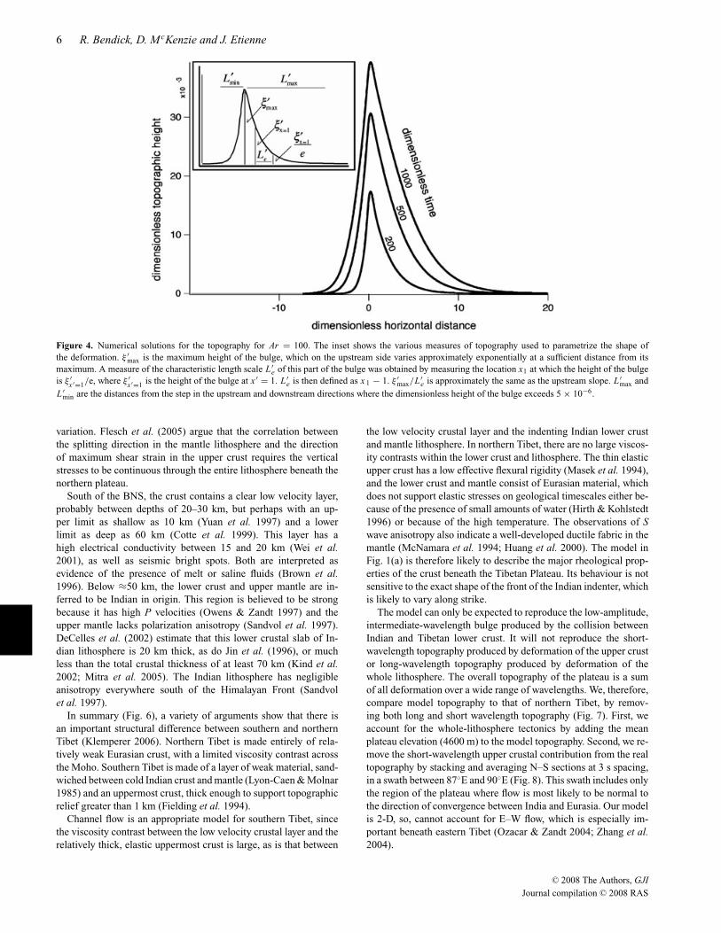
Figure 4. Numerical solutions for the topography for Ar = 100. The inset shows the various measures of topography used to parametrize the shape ofthe deformation. ξ ′

max is the maximum height of the bulge, which on the upstream side varies approximately exponentially at a sufficient distance from itsmaximum. A measure of the characteristic length scale L ′

e of this part of the bulge was obtained by measuring the location x1 at which the height of the bulgeis ξ ′

x ′=1/e, where ξ ′x ′=1 is the height of the bulge at x ′ = 1. L ′

e is then defined as x 1 − 1. ξ ′max/L ′

e is approximately the same as the upstream slope. L ′max and

L ′min are the distances from the step in the upstream and downstream directions where the dimensionless height of the bulge exceeds 5 × 10−6.

variation. Flesch et al. (2005) argue that the correlation betweenthe splitting direction in the mantle lithosphere and the directionof maximum shear strain in the upper crust requires the verticalstresses to be continuous through the entire lithosphere beneath thenorthern plateau.

South of the BNS, the crust contains a clear low velocity layer,probably between depths of 20–30 km, but perhaps with an up-per limit as shallow as 10 km (Yuan et al. 1997) and a lowerlimit as deep as 60 km (Cotte et al. 1999). This layer has ahigh electrical conductivity between 15 and 20 km (Wei et al.2001), as well as seismic bright spots. Both are interpreted asevidence of the presence of melt or saline fluids (Brown et al.1996). Below ≈50 km, the lower crust and upper mantle are in-ferred to be Indian in origin. This region is believed to be strongbecause it has high P velocities (Owens & Zandt 1997) and theupper mantle lacks polarization anisotropy (Sandvol et al. 1997).DeCelles et al. (2002) estimate that this lower crustal slab of In-dian lithosphere is 20 km thick, as do Jin et al. (1996), or muchless than the total crustal thickness of at least 70 km (Kind et al.2002; Mitra et al. 2005). The Indian lithosphere has negligibleanisotropy everywhere south of the Himalayan Front (Sandvolet al. 1997).

In summary (Fig. 6), a variety of arguments show that there isan important structural difference between southern and northernTibet (Klemperer 2006). Northern Tibet is made entirely of rela-tively weak Eurasian crust, with a limited viscosity contrast acrossthe Moho. Southern Tibet is made of a layer of weak material, sand-wiched between cold Indian crust and mantle (Lyon-Caen & Molnar1985) and an uppermost crust, thick enough to support topographicrelief greater than 1 km (Fielding et al. 1994).

Channel flow is an appropriate model for southern Tibet, sincethe viscosity contrast between the low velocity crustal layer and therelatively thick, elastic uppermost crust is large, as is that between

the low velocity crustal layer and the indenting Indian lower crustand mantle lithosphere. In northern Tibet, there are no large viscos-ity contrasts within the lower crust and lithosphere. The thin elasticupper crust has a low effective flexural rigidity (Masek et al. 1994),and the lower crust and mantle consist of Eurasian material, whichdoes not support elastic stresses on geological timescales either be-cause of the presence of small amounts of water (Hirth & Kohlstedt1996) or because of the high temperature. The observations of Swave anisotropy also indicate a well-developed ductile fabric in themantle (McNamara et al. 1994; Huang et al. 2000). The model inFig. 1(a) is therefore likely to describe the major rheological prop-erties of the crust beneath the Tibetan Plateau. Its behaviour is notsensitive to the exact shape of the front of the Indian indenter, whichis likely to vary along strike.

The model can only be expected to reproduce the low-amplitude,intermediate-wavelength bulge produced by the collision betweenIndian and Tibetan lower crust. It will not reproduce the short-wavelength topography produced by deformation of the upper crustor long-wavelength topography produced by deformation of thewhole lithosphere. The overall topography of the plateau is a sumof all deformation over a wide range of wavelengths. We, therefore,compare model topography to that of northern Tibet, by remov-ing both long and short wavelength topography (Fig. 7). First, weaccount for the whole-lithosphere tectonics by adding the meanplateau elevation (4600 m) to the model topography. Second, we re-move the short-wavelength upper crustal contribution from the realtopography by stacking and averaging N–S sections at 3 s spacing,in a swath between 87◦E and 90◦E (Fig. 8). This swath includes onlythe region of the plateau where flow is most likely to be normal tothe direction of convergence between India and Eurasia. Our modelis 2-D, so, cannot account for E–W flow, which is especially im-portant beneath eastern Tibet (Ozacar & Zandt 2004; Zhang et al.2004).




1

1.5

2

2.5

-0.8

-0.6

-0.4

-0.2

00.2

0.4

0.6

0.8

1

1.2

1.4

1.6

1

1.5

2

2.5

-0.8

-0.6

-0.4

-0.2

0

-2.6

-2.4

-2.2

-2

-1.8

-1.6

-1.4

-1.2

-1

-0.8

second-order model

data

1

1.5

2

2.5

-0.8

-0.6

-0.4

-0.2

0

-2.2

-2

-1.8

-1.6

-1.4

-1.2

-1

-0.8

1

1.5

2

2.5

-0.8

-0.6

-0.4

-0.2

0

-0.04

-0.03

-0.02

-0.01

0

0.01

0.02

0.03

0.04

1

1.5

2

2.5

-0.8

-0.6

-0.4

-0.2

00.2

0.4

0.6

0.8

1

1.2

1.4

1.6

1

1.5

2

2.5

-0.8

-0.6

-0.4

-0.2

0

-0.1

-0.05

0

0.05

0.1

0.15

0.2

0.25

residuals

Figure 5. Surfaces fit to measurements of (a) the slope ξ ′max/L ′

e and (b) the skewness L ′max/L ′

min of the topography from model runs as functions of step ratioand Argand number. The individual measurements are shown with open circles. Plots of the polynomial fits, eqs (3) and (4), to the measurements in (a) and(b). Residuals between the numerical results and the polynomial fits. Note the change in vertical scale between (a)–(d) and (e) and (f).

4 T I B E TA N T O P O G R A P H Y F RO MC RU S TA L F L OW

The model and the observed, bandpassed topography both includea low-amplitude, long-wavelength bulge in the Qiangtang, north

of the Banggong Suture, which we interpret to be the topographicexpression of crustal flow resulting from the Indian indenter. Webelieve that the relatively low elevation of the BNS (Fig. 7) marksthe southern limit of topography excited by the intrusion of therigid Indian crust and lithosphere. The absence of intermediate




Figure 6. A cartoon cross-section showing lateral and vertical heterogeneity of the crust beneath Tibet. Rigid Indian crust and lithosphere penetrates Eurasianlower crust as far north as the Banggong–Nujiang Suture (BNS) region. In the southern plateau, a viscous crustal channel is confined between the Indianindenter and the thin elastic lid (hatched) at the surface. In the northern plateau, no strong viscosity contrast exists at depth.

Figure 7. Smoothed topography of the Tibetan Plateau. The region dominated by crustal flow is the region of low relief in the centre of the plateau. The swathused to generate topographic profile in Fig. 8 is shown as a blue box and was produced by averaging N–S profiles from 29◦N to 39◦N between 87◦E and 90◦E.ITS, the Indus − Tsangpo suture; BNS, the Banggong–Nujiang suture and ATF, the Altyn Tagh fault.

wavelength topography south of this limit is compatible with hor-izontal flow in the crust, since only the vertical component ofthe velocity generates topography. The maximum elevation in theQiangtang is located near 33.7◦N. According to our model, thiscorresponds to the position of the front of the indenter. This is>100 km north of most estimates of the northernmost limit of In-dian crust from seismic observations (e.g. Chen & Ozalaybey 1998;Tilmann et al. 2003; Ozacar & Zandt 2004).

The observed topographic profiles are used to estimate the posi-tion of the step and also Ar and relative step height through simul-taneous solutions of eqs (11) and (13). The shape of the Qiangtangbulge constrains the values of L max + L min, the slope, ξ max/L e, andthe skewness, L max/L min. We used these estimates to calculate Arand a/h, using eqs (11) and (13). This approach gives an Argandnumber of about 1500 and a dimensionless step height of 0.3. Usingthis value of Ar, we calculate the viscosity of the flowing crust fromeq. (8) and estimates of the values of the other parameters. The mean

crustal density for central Tibet is taken to be 2.9 Mg m−3 (Haineset al. 2003) and g is 9.8 m s−2. We estimate that the thickness ofthe viscous layer can be no more than 60 km because the publishedMoho depths for central Tibet range from 50–78 km (Zhao et al.2001; Haines et al. 2003; Meissner et al. 2004) and the elastic lidthickness is <10 km (Masek et al. 1994). The total relative ve-locity between the Indian indenter and the Tibetan lower crust is≈20 mm yr−1. This value is less than the total India–Eurasia con-vergence rate of 28–34 mm yr−1 (Zhang et al. 2004) because someof the relative motion is taken up by deformation north of Tibet.If the Argand number is 1500, these values give a viscosity of theTibetan middle and lower crust of 1020 Pa s, in general agreementwith other bounds on crustal viscosity (Meissner & Kusznir 1987;Masek et al. 1994; Flesch et al. 2001; Copley & McKenzie 2007).The fit between the model and observed topography is satisfactoryfor Argand numbers between 1200 and 1700, corresponding to aviscosity range from 0.8 × 1020 to 1.1 × 1020 Pa s. The thickness




Figure 8. Mean topography of the Qiangtang bulge from the swath shownin Fig. 7 (blue), compared with the best fitting model (red) with Ar=1500,a/h = 0.3 and h = 60 km.

of the viscous region and the convergence velocity between the in-denter and the Indian lower crust are probably the least well knownof the partameters involved. Reasonable bounds on layer thicknessare 40–60 km and between 15 and 30 mm yr−1 for the convergencevelocity. Using these values, the acceptable range of lower crustalviscosities increases to 1 × 1020 ± 0.3 × 1020 Pa s. A dimensionlessstep size of 0.3 gives a thickness for the Indian crustal indenter of20 km, in agreement with independent estimates from seismology(Brown et al. 1996; Sandvol et al. 1997) and gravity (Jin et al. 1996).Our estimate of the viscosity of the low-viscosity layer beneathTibet agrees with that of 1020 Pa s obtained by Copley & McKenzie(2007). They modelled the GPS velocities across the Himalayanfront as a gravity-driven flow. They also showed that this value forthe viscosity is compatible with the creep properties of crustal rocksat temperatures of 700–900 ◦C.

5 D I S C U S S I O N

The models for crustal flow, under conditions of convergence pre-sented here, apply to any region with compressive boundary condi-tions, where part of the crust is sufficiently weak for solid-state flowto occur and where the structure suggests that large lateral variationsin rheology are present. The solutions we have obtained for lowercrustal flow over a step require the vertical stress to be continuousthrough the lithosphere. The topographic effects of the flow de-scribed here are sufficiently large in amplitude to be observed at thesurface and to be separated from both shorter wavelength featuressupported by elastic forces in the upper crust and longer wavelengthfeatures generated by distributed deformation of the whole litho-sphere. The shape of topography supported by lower crustal flowcan be used to estimate the geometry of a crustal indenter and theviscosity of the lower crust.

In the case of Tibet, a model of flow over a rigid, undeformableindenter reproduces the elevation, slope and asymmetry of the el-evation in the Qiangtang region of Tibet, which is associated withthe northern limit of Indian lithosphere. The model is 2-D, andtherefore, cannot describe the eastward component of flow or anyE–W variations in mechanical properties. The shape of the inden-ter is also likely to be more complicated than that modelled hereand may vary significantly along strike. These 3-D effects may be

responsible for the discrepancy between seismic estimates of thegeographic position of Indian lower crust and mantle lithosphereand our estimate from the topography.

The topography of northern Tibet sets an upper bound on thenorthern extent of the Indian indenter near 33.7◦N and on the vis-cosity of the lower crust beneath northern Tibet of 1.3 × 1020 Pa s.The model also provides an estimate of 20 km for the thickness ofthe Indian crust that is present beneath southern Tibet.

A C K N OW L E D G M E N T S

The NERC COMET programme supported this research. RB thanksJ. Jackson, P. England, B. Parsons and J. Li for suggestions andsupport, A. Copley for generating Fig. 7 and L. Royden and C.Beaumont for their useful reviews.

R E F E R E N C E S

Beaumont, C., Jamieson, R., Nguyen, M. & Medvedev, S., 2004. Crustalchannel flows, 1: numerical models with applications to the tectonics ofthe Himalayan–Tibetan orogen, J. geophys. Res., 109, B06406.

Bendick, R. & Flesch, L., 2007. Reconciling lithospheric deformation andlower crustal flow beneath central Tibet, Geology, 35, 895–898.

Brace, W. & Kohlstedt, D., 1980. Limits on lithospheric stress imposed bylaboratory experiments, J. geophys. Res., 85, 6248–6252.

Braitenberg, C., Wang, Y., Fang, J. & Hsu, H., 2003. Spatial variations offlexure parameters over the Tibet–Quinghai plateau, Earth planet. Sci.Lett., 205, 211–224.

Brezzi, F. & Fortin, M., 1991. Mixed and Hybrid Finite Elements Methods,Springer-Verlag, New York.

Brown, L. et al., 1996. Bright spots, structure, and magmatism in southernTibet from INDEPTH seismic reflection profiling, Science, 274, 1688–1691.

Burov, E. & Diament, M., 1995. The effective elastic thickness (Te) ofcontinental lithosphere: what does it really mean?, J. geophys. Res., 100,3905–3927.

Chen, W. & Ozalaybey, S., 1998. Correlation between seismic anisotropy andBouguer gravity anomalies in Tibet and its implications for lithosphericstructures, Geophys. J. Int., 135, 93–101.

Clark, M. & Royden, L., 2000. Topographic ooze: building the easternmargin of Tibet by lower crustal flow, Geology, 28, 703–706.

Copley, A. & McKenzie, D., 2007. Models of crustal flow in the India-Asiacollision zone, Geophys. J. Int., 169, 683–698.

Cotte, N., Pedersen, H., Campillo, M., Mars, J., Ni, J., Kind, R., Sandvol,E. & Zhao, W., 1999. Determination of the crustal structure in southernTibet by dispersion and amplitude analysis of Rayleigh waves, Geophys.J. Int., 138, 809–819.

DeCelles, P., Robinson, D. & Zandt, G., 2002. Implications of shortening inthe Himalayan fold-thrust belt for uplift of the Tibetan plateau, Tectonics,21, 1062.

Fielding, E., Isacks, B., Barazangi, M. & Duncan, C., 1994. How flat isTibet? Geology, 22, 163–167.

Flesch, L., Haines, A.J. & Holt, W., 2001. Dynamics of the India-Eurasiacollision zone, J. geophys. Res., 106, 16 435–16 460.

Flesch, L., Holt, W., Silver, P., Stephenson, M., Wang, C. & Chao, W., 2005.Constraining the extent of crust-mantle coupling in central Asia usingGPS, geologic, and shear-wave splitting data, Earth planet. Sci. Lett.,238, 248–268.

Fortin, M. & Glowinski, R., 1983. Augmented Lagrangian Methods, Appli-cations to the Numerical Solution of Boundary Value Problems, ElsevierScience, Amsterdam.

Haines, S., Klemperer, S., Brown, L., Guo, J., Mechie, J., Meissner, R.,Ross, A. & Zhao, W., 2003. INDEPTH III seismic data: from surfaceobservations to deep crustal processes in Tibet, Tectonics, 22, 1001.




Hirth, G. & Kohlstedt, D., 1996, Water in the oceanic upper mantle: impli-cations for rheology, melt extraction, and the evolution of the lithosphere,Earth planet. Sci. Lett., 144, 93–108.

Hood, P. & Taylor, C., 1973. A numerical solution of the Navier-Stokesequations using the finite element technique, Comput. Fluids, 1, 73–100.

Houseman, G. & England, P., 1986. Finite strain calculations of continen-tal deformation, 1: method and general results for convergent zones, J.geophys. Res., 91, 3651–3663.

Huang, W. et al., 2000. Seismic polarization anisotropy beneath the centralTibetan Plateau, J. geophys. Res., 105, 27 979–27 989.

Jackson, J., Austrheim, H., McKenzie, D. & Priestley, K., 2004. Metastabil-ity, mechanical strength, and the support of mountain belts, Geology, 32,625–628.

Jin, Y., McNutt, M. & Zhu, Y., 1996. Mapping the descent of Indian andEurasian plates beneath the Tibetan Plateau from gravity anomalies, J.geophys. Res., 101, 11 275–11 290.

Kind, R. et al., 2002. Seismic images of crust and upper mantle be-neath Tibet: evidence for Eurasian plate subduction, Science, 298, 1219–1221.

Klemperer, S., 2006. Crustal flow in Tibet: geophysical evidence for thephysical state of Tibetan lithosphere, and inferred patterns of active flow,in Channel Flow, Ductile Extrusion, and Exhumation in Continental Col-lision Zones, Vol. 268, p. 39–70, eds Law, R.D., Searle, M.P. & Godin,L., Spec. Publ. Geological Society, London.

Lyon-Caen, H. & Molnar, P., 1985, Gravity anomalies, flexure of the IndianPlate, and the structure, support and evolution of the Himalaya and GangaBasin, Tectonics, 4, 513–538.

Maggi, A., Jackson, J., McKenzie, D. & Priestley, K., 2000. Earthquakefocal depths, effective elastic thickness, and the strength of the continentallithosphere, Geology, 28, 495–498.

Masek, J., Isacks, B. & Fielding, E., 1994. Rift flank uplift in Tibet: evidencefor a viscous lower crust, Tectonics, 13, 659–667.

McKenzie, D., 2003. Estimating T e in the presence of internal loads, J.geophys. Res., 102, 2438.

McKenzie, D. & Jackson, J., 2002. Conditions for flow in the lower crust,Tectonics, 21, doi:10.1029/2002TC001394.

McKenzie, D., Nimmo, F., Jackson, J., Gans, P. & Miller, E., 2000. Char-acteristics and consequences of flow in the lower crust, J. geophys. Res.,105, 11 029–11 046.

McKenzie, D., Jackson, J. & Priestley, K., 2005. Thermal structure ofoceanic and continental lithosphere, Earth planet. Sci. Lett., 233, 337–349.

McNamara, D., Owens, T., Silver, P. & Wu, F., 1994. Shear wave anisotropybeneath the Tibetan Plateau, J. geophys. Res., 99, 13 655–13 665.

McNamara, D., Owens, T. & Walter, W., 1995. Observations of regionalphase propagation across the Tibetan Plateau, J. geophys. Res., 100,22 215–22 229.

Meade, B., 2007. Present–day kinematics at the India–Asia collision zone,Geology, 35, 81–84.

Meissner, R. & Kusznir, N., 1987. Crustal viscosity and the reflectivity ofthe lower crust, Ann. Geophysicae, Ser. B, 5, 365–373.

Meissner, R., Tilmann, F. & Haines, S., 2004. About the lithospheric struc-ture of central Tibet, based on seismic data from the INDEPTH III profile,Tectonophysics, 380, 1–25.

Mitra, S., Priestley, K., Bhattacharyya, A. & Gaur, V., 2005. Crustal structureand earthquake focal depths beneath Northeastern India and southernTibet, Geophys. J. Int., 160, 227–248.

Owens, T. & Zandt, G., 1997. Implications of crustal property variations formodels of the Tibetan Plateau evolution, Nature, 387, 37–43.

Ozacar, A. & Zandt, G., 2004. Crustal seismic anisotropy in central Tibet:implications for deformational style and flow in the crust, Geophys. Res.Lett., 31, L23601.

Royden, L., 1996. Coupling and decoupling of crust and mantle in conver-gent orogens: implications for strain partitioning in the crust, J. geophys.Res., 101, 17 679–17 705.

Sandvol, E., Ni, J., Kind, R. & Zhao, W., 1997. Seismic anisotropy be-neath the southern Himalayas–Tibet collision zone, J. geophys. Res., 102,17 813–17 823.

Saramito, P., Roquet, N. & Etienne, J., 2006. RHEOLEF open-source free software, available at http://www-lmc.imag,fr/lmc-edp/Pierre.Saramito/rheolef.

Shapiro, N. & Ritzwoller, M., 2002. Monte-Carlo inversion for a globalshear- velocity model of the crust and upper mantle, Geophys. J. Int., 151,88–105.

Tapponnier, P., Xu, Z., Roger, F., Meyer, B., Arnaud, N., Wittlinger, G. &Yang, J., 2001. Oblique stepwise rise and growth of the Tibet Plateau,Science, 294, 1671–1677.

Thatcher, W., 2006, Microplate model for present-day deformation of Tibet,J. geophys. Res., 112, B01401.

Tilmann, F., Ni, J. & INDEPTH, III Seismic Team., 2003. Seismic imagingof the downwelling Indian lithosphere beneath Central Tibet, Science,300, 1424–1427.

Vanderhaeghe, O., Medvedev, S., Fullsack, P., Beaumont, C. & Jamieson,R., 2003. Evolution of orogenic wedges and continental plateaux; insightsfrom crustal thermal-mechanical models overlying subducting mantlelithosphere, Int. Geol. Rev., 44, 39–61.

Wei, W. et al., 2001. Detection of widespread fluids in the Tibetan crust bymagnetotelluric studies, Science, 292, 716–718.

Yuan, X., Ni, J., Kind, R., Mechie, J. & Sandvol, E., 1997. Lithospheric andupper mantle structure of southern Tibet from a seismological passivesource experiment, J. geophys. Res., 102, 27 491–27 500.

Zhang, P. et al., 2004. Continuous deformation of the Tibetan plateau fromglobal positioning system data, Geology, 32, 809–812.

Zhao, W. et al., 2001. Crustal structure of central Tibet as derived fromproject INDEPTH wide-angle seismic data, Geophys. J. Int., 145, 486–498.

A P P E N D I X : A N A NA LY T I C S O LU T I O N

The analytic solution to the viscous flow problem shown in Fig. 1is straightforward to obtain if a = h and the shear stess, rather thanw, is zero on �5, because the flow driven by the rigid motion of thetop and bottom of the viscous layer does not alter the pressure whengravity is absent. This result allows the solutions that McKenzieet al. (2000) obtained to a similar problem, to be used to calculatethe time-dependent behaviour. All the variables in this Appendixare dimensionless and the primes are omitted.

The thickness of the layer is ξ − ζ , where ξ (x , t) is the upper andζ (x , t) is the lower boundary. The kinematic condition requires therate of change of the thickness of the layer to equal the differencebetween the top and bottom vertical velocity,

d

dt(ξ − ζ ) = wz=1 − wz=0. (A1)

If the layer is to be isostatically compensated,

ζ = −(

1

R − 1

)ξ (A2)

and eq. (A1) becomes(R

R − 1

)dξ

dt= wz=1 − wz=0. (A3)

It is convenient to separate p into a lithostatic part, 1 − z and aperturbation p1,

p = 1 − z + p1. (A4)

Then eqs (5) and (6) become

∇ · v = 0, (A5)

∇2v = ∇ p1. (A6)




We seek a 2-D solution to these equations using a stream functionψ :

v = (u, w) =(

−∂ψ

∂z,∂ψ

∂x

), (A7)

which satisfies eq. (A5). Taking the curl of eq. (A6),

∇4ψ = 0. (A8)

The boundary conditions become

−(

∂ψ

∂z

)z=0,1

= − 1

Ar, (A9)

σzz = 0 = −pz=1+ξ + 2

(∂2ψ

∂x∂z

)z=1

. (A10)

Since eq. (A9) requires ∂ψ/∂ z to be constant on both boundaries,eq. (A10) becomes

p1(z=1) = ξ. (A11)

The shear stress on x = 0 requires[−∂2ψ

∂z2+ ∂2ψ

∂x2

]x=0

= 0. (A12)

Since u = 0 on x = 0, (∂ψ/∂ z)x=0 = 0. Eq. (A12) therefore requires[∂2ψ

∂x2

]x=0

= 0 (A13)

or, equivalently,[∇2ψ]

x=0= 0. (A14)

The pressure p1 is obtained by integration of eq. (A6)

∂p1

∂x= −∇2 ∂ψ

∂z(A15)

or

∂p1

∂z= ∇2 ∂ψ

∂x. (A16)

A suitable solution to eq. (A8) is

ψ = F(x, z) + G(x, z) + z

Ar, (A17)

where

F(x, z) = (A1 + B1x)e−k1x cos k1z,

G(x, z) = [(A2 + B2z)e−k2z + (C2 + D2z)ek2z

]sin k2x, (A18)

and k1 and k2 are the vertical and horizontal wavenumbers, respec-tively. G is the same function as McKenzie et al. (2000, eqs A5 andA6) obtained. The condition σ xz = 0 on x = 0 requires B 1 = 0,when ∇2 F = 0 everywhere. eqs (A15) and (A16) then show that p1

is independent of F and depends only on G. The horizontal velocity

−∂ψ/∂z on z = 0, 1 is −1/Ar if ∂ F/∂z and ∂G/∂z are zero onthese boundaries. The first condition requires

sin k1 = 0 or k1 = nπ. (A19)

The second leads to the same expressions for rigid boundary condi-tions discussed by McKenzie et al. (2000). The boundary conditionu = 0 on x = 0 requires

− 1

Ar+

∞∑n=1

nπ A1(n) sin nπ z = 0. (A20)

Eq. (A20) requires that A1(n) = 0 if n is even, and

A1(m) = 4

k2m Ar

, km = (2m + 1)π, (A21)

when n(=2m + 1) is odd. Therefore, the boundary conditions canonly be satisfied by discrete values of k1. The final boundary con-dition, eq. (A3), requires(

R

R − 1

)dξ

dt=

(∂G

∂x

)z=1

−(

∂G

∂x

)z=0

+ H, (A22)

where

H =(

∂ F

∂x

)z=1

−(

∂ F

∂x

)z=0

= 8

Ar

∞∑m=0

e−km x

km, (A23)

H is a function of x but not of t. Fourier transforming eqs (A22) and(A23) with respect to x gives(

R

R − 1

)dξ

dt=

(∂G

∂x

)z=1

−(

∂G

∂x

)z=0

+ H , (A24)

where the bars denote transformed variables. ξ and G are functionsof t, but H is a constant. McKenzie et al. showed that the solutionto this equation when H = 0 is

ξ = ξ 0e−t/τ (A25)

and obtained expressions for τ (k). When H = 0, the solution toeq. (A24) is

ξ = ξ 0

(1 − e−t/τ

), (A26)

where

ξ 0 =(

R − 1

R

)τ H . (A27)

The Fourier transforms, to obtain H from H using eq. (A23) andξ (t) from ξ (t) using eq. (A26), were carried out numerically. Thesolution is only valid when ξ , ζ � 1. Since we are interested in thelong wavelength behaviour, we used the expression for τ when k �1 for rigid boundary conditions on z = 0, 1 (McKenzie et al. 2000,A22):

τ = 3R

k2(R − 1). (A28)



topography associated with crustal flow in continental...

Documents