Exercise EX 3.2

1

Topic Determination of fault-plane solutions by hand Authors Peter Bormann and Michael Baumbach ()(formerly

GeoForschungsZentrum Potsdam, Department 2: Physics of the Earth, Telegrafenberg, D-14473 Potsdam, Germany); E-mail: pb65@gmx.net; Siegfried Wendt, Geophysical Observatory Collm, University of Leipzig, D-04779 Wermsdorf, Germany, E-mail: wendt@rz.uni-leipzig.de

Version June 2012; DOI: 10.2312/GFZ.NMSOP-2_EX_3.2 1 Aim Fault-plane solutions are nowadays routinely calculated and plotted by a diversity of software programs. They may result from using different types of seismic waves, recorded in different frequency bands and ranges of epicentral distances and by measuring and analyzing different record parameters. Accordingly, such solutions, may be based on more sophisticated optimal waveform fitting between real and synthesized records, on considering azimuthal variations in amplitude ratios between P and S waves, or on simple “classical” P-wave first-motion polarity readings only. The latter is still the most common procedure for masses of data, especially when recorded in the local distance and low magnitude range. However, the under-laying assumptions, sequential procedural steps and ranges of possible errors of fault-plane solutions are often not sufficiently well known to the common user of such data and programs. Therefore, it is recommendable that at least once the step-by-step determination of a fault-plane solution by hand, based on first-motion polarity readings, should be part of the educational program of any future seismologist or geoscientist, as an eye-opening and awareness creating exercise. For this we have selected a realistic yet not too simple and data-wise not too ideally constrained example based on recordings of local aftershocks. The exercise aims at:

• understanding how fault slip affects the polarities of P waves; • understanding, how the applied crustal model in the source location process may

influence the calculated take-off angles as a function of epicentral distance; • understanding the presentation of P-wave polarities in an equal angle Wulff net or

an equal area projection (Lambert-Schmidt net) of the focal sphere; • constructing a fault-plane solution and determining the related parameters (P and T

axes and displacement vector) for a real earthquake; • relating the directions of the fault-plane solutions to the tectonic setting and

complementary information on the regional stress pattern. 2 Data and procedures Before a fault-plane solution for a teleseismic event can be constructed, the following steps must be completed: a) Interpretation of P-wave first-motion polarities from seismograms at several stations;

Exercise EX 3.2

2

b) Calculation of epicentral distances and source-to-station azimuths for these stations; c) Calculation of the take-off angles Θ for the seismic P-wave rays leaving the hypocenter

towards these stations. Both b) and c) require the knowledge of the focal depth and of the P-wave velocity-depth function along the ray path (see EX 3.3). Commonly, standard Earth velocity models are used (e.g., Kennett, 1991 or AK135, Kennett et al., 1995; see DS 2.1), especially, when teleseismic recordings are analyzed. Most location programs provide both the source-station azimuths and take-off angles in their output files. In the case of local events, however, it is necessary to determine beforehand, which P-wave travel-time branch is arriving first at what distance. This is strongly influenced by the velocity model of the local crust. Therefore, the events should be located, if possible, with a layered velocity model that is represents reasonably well the Earth crust of that region. If it deviates significantly from the global model, significantly biased take-off angles from the source may be calculated for the first arriving P-wave rays. This may result in not separable polarity patterns and thus inconsistent or biased fault-plane solutions. The exercise below is based on related general definitions, relationships and diagrams presented in Chapter 3 of this Manual in the section “Determination of fault-plane solutions.” The starting data for the exercise are summarized in Table 1. They relate to a locally recorded aftershock of the Ms = 6.8 Erzincan earthquake in Turkey (Main shock: 13.03.1992, 39.72°N, 39.63°E; aftershock: 12.04.1992, Ml = 2.8 , 39.519° N, 39.874° E, source depth h = 3 km). The distances of the recording stations range from 3.7 km to 49.6 km They were calculated according to steps a)-c) by using the program HYPO71 (Lee and Lahr, 1975). Note: In the special case of a near surface source in a homogeneous or a plane layered velocity model the take-off angles Θ from the source agree with the angle of incidence AIN calculated with HYPO71 for the respective seismic ray arriving at a given station. Figure 1 defines Θ, which depends on source distance, source depth, velocity model and the recorded first arriving type of P wave. Further, for an average single layer crustal model of 30 to 40 km thickness, all P-wave first arrivals within a distance of about 120 km to < 200 km are Pg and up-going. That is, they emerge only from the upper half of the focal hemisphere. Also, when using HYPO71 with the average global two-layer crust according to the velocity model IASP91 (Kenneth 1991) only upper hemisphere take-off angles would have been calculated for the first P-wave arrivals up to distances of 50 km. But in the epicentral area under consideration a significant velocity increase in the upper crust was already found at 4 km depth (increase of vp = 5.3 km/s to 6.0 km/s). Therefore, a single-layer model above half-space for the upper crust had to be used in the calculations. Accordingly, only stations up to 17 km distance were reached by first arriving rays that left through the upper focal sphere. At larger distances the first arriving P waves had left the lower focal sphere. They were refracted back at this upper crustal discontinuity under the critical angle of incidence icr, which is in our layer model 62° according to the velocity contrast v1/v2 = 5.3/6.0 = sinicr = sinΘcr. These critically refracted P-waves travel with a constant apparent horizontal velocity of 6.0 km/s and therefore arrive at stations beyond 17 km epicentral distance also with a constant incidence angle AINcr = 62° (Figure 2). Fault-plane solutions are derived by remapping the penetration points of seismic rays through the upper and lower hemisphere on a suitable horizontal plane net projection and separating from each other sectors of opposite polarity by pairs of orthogonal great circles. However, as

Exercise EX 3.2

3

obvious from Figures 1 and 2, the polarities of rays leaving the upper and lower hemisphere with the same azimuth are mirrored. Mapping them both with their originally calculated values Θ and azimuth AZM on the same horizontal net projection would result in incompatible polarity plots. Therefore, one has to make up ones mind, whether one uses only upper or lower hemisphere polarities and has then to mirror the other hemisphere data so that they become compatible with the reference hemisphere data. For the exercise we use only lower hemisphere data, as generally used when analyzing teleseismic polarity readings. Thus, for all upper hemisphere polarities with 90° < Θ ≤ 180° corrected values Θc and AZMc have to be calculated by using the relationships given in Figure 1. Only these corrected upper hemisphere polarities can be plotted jointly with the original lower hemisphere polarities (0° ≤ Θ ≤ 90°) on the same net projection. Table 1 Original and corrected (not yet calculated) values of ray azimuth (AZM and AZMc) and take-off angles (Θ and Θc, respectively) towards stations of a temporary network at epicentral distance DIS which recorded the Erzincan aftershock of April 12, 1994. POL - polarity of P-wave first motions. D = down = negative (-) first half-wave and U = up = positive (+) first half-wave in vertical component records.

STA DIST (km)

AZM (degree)

Θ (degree)

POL AZMc (degree)

Θc (degree)

ALI ME2 KAN YAR ERD DEM GIR UNK SAN PEL GUN ESK SOT BA2 MOL YUL ALT GUM GU2 BAS BIN HAR KIZ AKS SUT

3.7 7.1 7.7 8.2

13.6 14.3 14.4 16.2 17.2 18.6 22.6 22.7 23.8 27.3 28.8 29.3 31.5 32.0 32.0 35.6 36.4 38.7 42.2 48.7 49.6

40 134 197 48 313 330 301 336 76 327 290 312 318 79 297 67 59 320 320 308 295 24 311 284 295

130 114 112 111 103 102 102 101 62 62 62 62 62 62 62 62 62 62 62 62 62 62 62 62 62

D D D D D D U D U D U U D U U U D U D D U D U D U

Exercise EX 3.2

4

Figure 1 Transformation of a ray leaving the focal sphere upwards with a take-off angle Θ between 90° < Θ ≤ 180° into an equivalent downward ray with same polarity but corrected take-off angle Θc and azimuth AZMc.

Figure 2 Two rays, leaving the focal sphere in opposite directions, reach - because of the symmetry of radiation pattern - the stations 1 and 2 with the same polarity. The crossing point of the up-going ray with the focal sphere can, therefore, be remapped according to the formulas given in Figure 1 into a crossing point with the lower hemisphere which coincides with the ray crossing-point for station 2.

Exercise EX 3.2

5

Note: Θ calculations based on strongly biased velocity models might result in inconsistent fault-plane solutions or not permit a proper separation of opposite polarity readings into quadrants (as in Figure 4) at all. The primary data in Table 1 were taken from the output file of the program HYPO71 with which the event was located. The first five columns of this file contain, as an example for the two stations ALI and ESK in Table 1, the following data: STN DIST AZM AIN PRMK ALI 3.7 40 130 IPD0 ESK 22.7 312 62 IPU1

with STN - station code; DIST - epicentral distance in km; AZM - azimuth towards the station clockwise in degree from north; AIN (replaced by us by Θ) - take-off angle of the ray leaving the source towards the station, measured as in Figure 1, and calculated for the given structure-velocity model; PRMK - P-wave reading remarks. In the column PRMK P stands for P-wave onset, I for impulsive (sharp) or E for emergent (less clear) onset, D for clear (or − for poor) downward first motion, U for clear (or + for poor) upward first motion as read at the station. The last character may range between 0 and 4 and is a measure of the quality (clarity) of the onset and thus of the weight given to the reading in the calculation procedure, e.g., 4 for zero weight and 0 for full weight. In case of the above two stations the values for ALI would need to be corrected to get the respective values for the equivalent lower hemisphere ray, i.e., Θc = 180° - 130° = 50° and AZMc = 180° + 40° = 220° while the values for ESK can be taken unchanged from the HYPO71 output file. The P-wave polarities are commonly plotted according to the take-off angles and azimuths of their rays on either the Wulff or the Lambert-Schmidt net (Figures 3a and b; Aki and Richards, 1980, Vol. 1, p. 109-110). The latter yields less cluttered data plots when Θ < 45°, but in principle the fault planes are constructed in the same manner (see EX 3.3).

a

b Figure 3 a) the equal-angle Wulff net and b) the equal-area Lambert-Schmidt net.

Exercise EX 3.2

6

The following relationships hold between the radius r (in cm) of the respective nets and the distance d (in cm) from the net center at which the take-off angle Θ has to be mapped in the direction of the azimuth AZM: Wulff net: d = r · tan(Θ/2); Lambert-Schmidt net: d = r · sin(Θ/2). Note: In both projections only the equator and the meridians are great circles. Also: All cut traces of the (possible) fault plane(s) through the focal sphere, which separate the segments of opposite polarity observations, have to be great circles. The amplitude radiation pattern of point source foci is commonly assumed to be spherically symmetric (Figure 4). For deviations see Chapter 3.

Figure 4 Radiation pattern of the radial displacement component (P wave) due to a double-couple source: a) for a plane of constant azimuth (with lobe amplitudes proportional to sin2θ) and b) over a sphere centered on the origin. Plus and minus signs of various sizes denote amplitude variation (with the spherical coordinates θ and φ) of outward (+; extensional quadrant) and inward (-; compressional quadrant) directed motions. The fault plane and auxiliary plane are nodal lines on which cosφ sin2θ = 0. The pair of open arrows in a) at the center denotes the shear dislocation and P and T in b) mark the penetration points of the pressure and tension axes, respectively, through the focal sphere. Note the alternating quadrants of inward (D, −) and outward directed motions (U, +); (modified from Aki and Richards 1980; with kind permission of the authors).

Exercise EX 3.2

7

According to the above, basically three steps are required for obtaining a fault-plane solution: (1) Calculating the positions of the penetration points of the seismic rays through the focal

sphere. They are defined by the azimuth AZM and the take-off angle Θ at which the ray leaves the source.

(2) Marking these penetration points through the upper or lower hemisphere in a horizontal projection of that sphere by using different symbols for upward U (+) and downward D (−) directed first motions of P waves in vertical component records. Usually, lower hemisphere projections are used. Rays which have left the upper hemisphere have to be transformed into their equivalent lower hemisphere rays. This is possible because of spherical symmetry of the radiation pattern (see Figure 4).

(3) Partitioning the projection of the lower focal sphere by two perpendicular great circles which separate all (or at least most) of the U (+) and D (−) arrivals in different quadrants.

Figure 5 shows the angles which describe the orientation and motion in space of a fault plane. The fault strike angle φs is measured clockwise against North ( 0° ≤ φs ≤ 360° ). To resolve the 180° ambiguity, it is assumed that when standing in the center of the net and looking into the strike direction of the fault it dips to the right hand side (i.e., its fault-trace projection is towards the right of the net center). The dip angle δ describes the inclination of the hanging wall against the horizontal ( 0° ≤ δ ≤ 90° ). The rake angle λ describes the displacement of the hanging wall relative to the foot wall ( -180° ≤ λ ≤ 180° ). λ = 0 corresponds to slip in strike direction, λ > 0 means upward motion of the hanging wall (i.e., reverse or thrust faulting component) and λ < 0 downward motion (i.e., normal faulting component). In other words: If the net center is located in the tension quadrant (+) or in the pressure quadrant (−) the fault has a thrust component or a normal component, respectively. The normal or thrust character of the fault-plane solution does not depend on which of the two nodal planes is the active fault plane.

Figure 5 Angles describing the orientation and motion of faults (see text).

Exercise EX 3.2

8

Figure 6 illustrates the measurement of these angles and of additional fault parameters in the net projections. P1, P2 and P3 mark the positions of the poles of the planes FP1 (fault plane), FP2 (auxiliary plane) and EP (equatorial plane) in their net projections. All three planes are perpendicular to each other (i.e., 90o apart) and intersect in the poles of the respective third plane, i.e., FP1 and FP2 in P3, FP1 and EP in P2 etc.

Figure 6 Determination of the fault plane parameters φs, δ and λ in the net diagrams. The polarity distribution, slip direction and projection of FP1 shown here correspond to the faulting case depicted qualitatively in Figure 4. Note: λ* = 180° - λ when the center of the net lies in the tension (+) quadrant (i.e., event with thrust component) or λ* = -λ when the center of the net lies in the pressure quadrant (i.e., event with normal faulting component. P1, P2 and P3 are the poles (i.e., 90° off) of FP1, FP2 and EP, respectively. P and T are the penetration points (poles) of the pressure and tension axes, respectively, through the focal sphere. + and − signs mark the quadrants with upward and downward P-wave first motions in vertical component records, respectively. Note: On the basis of polarity readings alone it can not be decided whether FP1 or FP2 was the active fault. Discrimination from seismological data alone is still possible but requires additional study of the directivity effects such as azimuthal variation of frequency (Doppler effect), amplitude ratios and/or waveforms (see Chapter 3). For sufficiently large shocks these effects can more easily be studied in low-frequency teleseismic recordings while in the local distance range, high-frequency waveforms and amplitudes may be strongly influenced by resonance effects due to low-velocity near-surface layers. Seismotectonic considerations or field evidence from surface rupture in case of strong shallow earthquakes as well as aftershock distribution may allow to resolve this ambiguity, too. For “cartoons” of several basic types of earthquake faulting and their related fault-plane solutions in so-called "beach-ball" presentations of the net projections see Chapter 3.

Exercise EX 3.2

9

3 Tasks Task 1: If in Table 1 Θ > 90°, then correct the take-off angles and azimuths in Table 1 for lower hemisphere projection: Θc = 180° - Θ, AZMc = AZM(<180°) + 180° or AZM(≥180°) - 180°. In case of Θ < 90° the original values remain unchanged. Task 2: Reproduce the Wulff net or the Lambert-Schmidt net projection in Figure 3, best on A4 paper with a radius r = 8 cm. Place a tracing paper or a transparency sheet over the net. Mark on it the center and perimeter of the net as well as the N, E, S and W directions. Pin the marked center of the transparency sheet with a needle to the center of the net copy on paper. Task 3: Mark the azimuth of the station on the perimeter of the transparency and rotate the latter until the tick mark is aligned along an azimuth of 0°, 90°, 180° or 270°. Measure the take-off angle Θ from the center of the net along this azimuth. This gives the intersection point of the particular P-wave ray with the lower hemisphere. Mark on this position the P-wave polarity with a distinct + for compression or ο for dilatation (U or D in Table 1) using different colors for better distinction of closely spaced polarities of different sign. Note: For calculating the proper distance d of the polarity entry from the center of the respective net you may also use the respective formulas given above for the Wulff net and the Lambert-Schmidt net as a function of r and Θ. In case that rays left the source through the upper hemisphere (Θ > 90°) Θc and AZMc for lower hemisphere projection have to be plotted. Task 4: Rotate the transparent sheet with the plotted data over the net and try to find a great circle (meridian on the net copy) which separates as good as possible the expected quadrants with different first motion signs. This great circle represents the intersection trace of one of the possible fault (or nodal) planes (FP1) with the lower half of the focal sphere. Note: Inconsistent polarities that are close to each other may be due to uncertainty in reading correctly the first motion direction of P-wave arrivals with low signal-to-noise ratio or to an incorrect velocity model for calculating the take-off angle. Yet, small P-wave amplitudes are to be expected for take-off angles near to the nodal (fault) planes. Thus, clusters of inconsistent polarities may guide your “eye fit” in finding the best separating great circle. Also computer programs for finding best fitting fault-plane solutions try to minimize both the number of misfitting polarities in the quadrants as well as their distance from the nodal plane. However, be aware that isolated inconsistent polarities may also be due to false polarity switching of the seismometer output or simply by reading errors on the seismic record. Task 5: Mark point A at the middle of the FP1 projection and find, perpendicular to FP1 and 90o apart, the pole P1 of FP1 (see Figure 6). All great circles, passing this pole are perpendicular to the FP1. Since the second possible fault (auxiliary) plane (FP2) must be perpendicular to the FP1, it has to pass P1. Find, accordingly, a great circle FP2 which again has to separate areas of different polarity.

Exercise EX 3.2

10

Task 6: Find the pole P2 for FP2 (which lies on FP1) and delineate the equatorial plane EP. The latter is perpendicular to both FP1 and FP2, i.e., it is a great circle through the poles P1 and P2. The intersection point of FP1 and FP2, P3, is the pole of the equatorial plane. Task 7: Mark the position of the poles of the pressure (P) and tension axes (T) on the equatorial plane and determine the direction of these axes towards (for P) and away from the center (for T) of the used net (see Figure 6). The poles for P and T lie on the equatorial plane in the center of the respective quadrants of downward (− or o) and upward (+) P-wave first motions, i.e., 45° away from the intersection points of the two fault planes with the equatorial plane. Note: All angles in the net projections have to be measured along great circles!

Task 8: Mark the slip vectors, connecting the intersection points of the fault planes with the equatorial plane, with the center of the considered net. If the center lies in a tension quadrant, then the slip vector points either from P2 on FP1 or from P1 on FP2 to the net center (see Figure 6). If it lies in a pressure quadrant, then the slip vectors points from the center in the opposite directions. The slip vector shows the direction of displacement of the hanging wall (see Figure 5). Task 9: Determine the azimuth (fault strike direction φs) of both FP1 and FP2. It is the angle measured clockwise against North between the directional vector connecting the center of the net with the end point of the respective projected fault trace lying towards the right of the net center (i.e., with the fault plane dipping towards the right; see Figure 6). Task 10: Determine the dip angle δ (measured from horizontal) for both FP1 and FP2 by putting their projected traces on a great circle. Measure δ as the difference angle from the outermost great circle (perimeter of the net) towards the considered fault-plane trace. Task 11:

Determine the slip direction (i.e., the sense of motion along the two possible fault planes. It is obtained by drawing one vector each from the center of the net to the poles P1 and P2 of the nodal planes (or vice versa from the poles to the center, depending on the sign of the rake angle λ). The vector from (or to) the center towards (or away from) P1 (P2) shows the slip direction along either FP2 or FP1. The rake angle λ is negative when it lies in the pressure (−) quadrant (event with a normal faulting component) and positive in case the center of the net lies in the tension (+) quadrant (i.e., an event with a thrust component) (Figure 7 top). In the first case holds λ = - λ* and in the second case λ = 180° - λ*. λ* has to be measured on the great circle of the respective fault plane between its crossing point with the equatorial plain and the respective azimuth direction of the considered fault plane (see Figure 6). For a pure strike slip motion (δ = 90°) λ = 0 defines a left lateral strike-slip and λ = 180° defines a right-

Exercise EX 3.2

11

lateral strike-slip which can also be interpreted as a left-lateral (counter-clockwise) or right-lateral (clockwise) “rotational” movement of the two blocks against each other (Figure 7 below). Note: If the slip on the first fault plane is left-lateral the slip on the second one is right-lateral and vice versa.

Figure 7 Basic types of earthquake faulting for some selected dip and rake angles. Mixed types of faulting occur when λ ≠ 0, 180o or ± 90o, e.g., normal faulting with strike-slip component or strike-slip with thrust component. Also, dip angles may vary between 0o < δ ≤ 90o. For fault-plane traces and polarity distributions of mixed faulting types in their "beach-ball presentation" see also Chapter 3, section Fault-plane solutions. Task 12: The azimuth of the pressure and the tension axes, respectively, is equal to the azimuth of the line connecting the center of the net through the poles of P and T with the perimeter of the net. Their plunge is the dip angle of these vectors against the horizontal (to be measured as for δ) (see Figure 6). Task 13: Insert your results of estimated fault-plane parameters as well as pressure and tension axes for the Erzincan aftershock into Table 2. Table 2 strike dip rake Fault plane 1 Fault plane 2

Exercise EX 3.2

12

azimuth plunge Pressure axis Tension axis Note: The angles may range between: 0° < strike < 360° 0° < azimuth < 360° 0° < dip < 90° 0° < plunge < 90° -180° < rake < 180° Task 14: The question which of the two nodal planes was the active fault plane, and hence the other the auxiliary plane, cannot be answered on the basis of the fault-plane solution alone. Considering the event in its seismotectonic context may give an answer. Therefore, we have marked the epicenter of the event in Figure 8 with an open star at the secondary fault F2 to the North Anatolian Fault (NAF).

Figure 7 Epicenters of aftershocks between March 21 and June 16, 1992 of the March 13, 1992 Erzincan earthquake, Turkey. The open circles represent the main shock (blue) and its strongest aftershock on March 15 (green), and the red star the analyzed aftershock. F1, F2 and F3 are secondary faults to the North Anatolian Fault (NAF). Black arrows - directions of relative plate motion, open arrows - direction of maximum horizontal compression as derived from centroid moment-tensor solutions of stronger earthquakes (modified Figure from Grosser et al., 1998).

Exercise EX 3.2

13

a) Decide which was the likely fault plane (FP1 or FP2)? b) What was the type of faulting? c) What was the direction of slip? and d) Is your solution compatible with the general sense of plate motion in the area as well with

the orientation of the acting fault and the orientation of stress/deformation in the area? 4 Solutions and discussion Taking it that you have carried out the exercise step-by-step yourself according to the above data, tasks and explanations, you may now compare your results, again step-by-step, with those which the authors of this exercise derived themselves by hand and or plotted them by using a computer program. The PC derived values are given in the summary parameter table in brackets. Fault planes determined by eye-fit to the polarity data may be uncertain by about ± 10o. This is acceptable. Even computer-assisted best fits to the data will produce different acceptable solutions within about the same error range with only slightly different standard deviations (e.g., Figure 1 in EX 3.3, comparing NEIC and HRVD solutions, respectively). But poor distribution of seismological stations (resulting in insufficient polarity data in several quadrants of the net diagram), erroneous polarity readings and/or differences in the velocity models used may result in still larger deviations between calculated and actual fault planes. One should also be aware that the assumed constant angular (45o) relationship between the fault plane on the one hand and the pressure and tension axis on the other hand is true in fact only in the case of a fresh rupture in a homogeneous isotropic medium. It may not be correct in the stress environment of real tectonic situations and for near surface sources in particular (i.e., P and T ≠ σ1 and -σ3, respectively; see discussion in section 3.1.2.6 of Chapter 3). Only the parameters of the fault plane are relatively reliable, provided that this applies also to the used velocity model. If, however, your polarity patterns and/or manually determined parameter values differ by more than about 20o from the solutions presented below or yield even a different type of faulting mechanism then you should critically check and correct your data entries and/or fault-plane fits. Solution 1, Task 1:

STA AZM (degree)

Θ (degree)

POL AZMc (degree)

Θc (degree)

ALI ME2 KAN YAR ERD DEM GIR UNK SAN PEL GUN ESK

40 134 197 48 313 330 301 336 76 327 290 312

130 114 112 111 103 102 102 101 62 62 62 62

D D D D D D U D U D U U

220 314 17 228 133 150 121 156

50 66 68 69 77 78 78 79

Exercise EX 3.2

14

SOT BA2 MOL YUL ALT GUM GU2 BAS BIN HAR KIZ AKS SUT

318 79 297 67 59 320 320 308 295 24 311 284 295

62 62 62 62 62 62 62 62 62 62 62 62 62

D U U U D U D D U D U D U

Solutions 2, Tasks 3-5, 9 and 10: Plotting polarities, finding FP1 and determining its strike and dip. Note that FP1 goes through a cluster of nearby conflicting polarities but separates well most of the + and – (•)signs.

Exercise EX 3.2

15

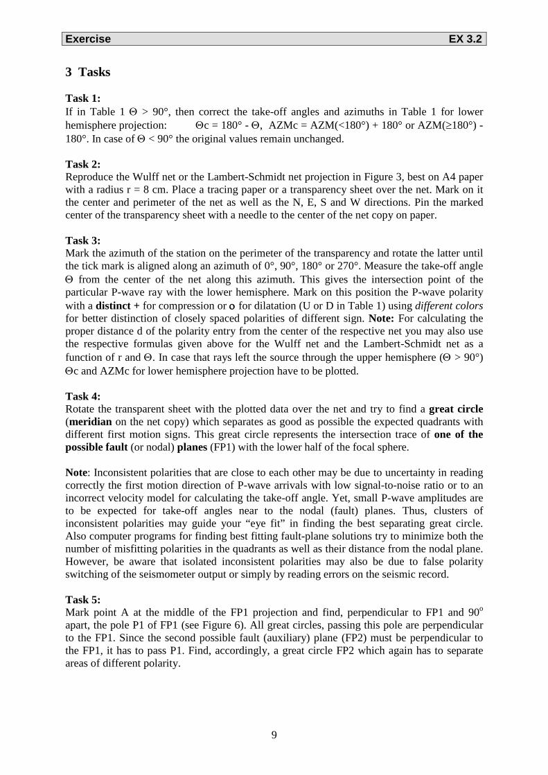
Solution 3, Task 6, 9 and 10: Finding FP2 and determining its strike and dip.

Solution 3, Task 7: Position of the poles on the equatorial plane EP of the pressure axis P (green) and tension axis T (red):

Exercise EX 3.2

16

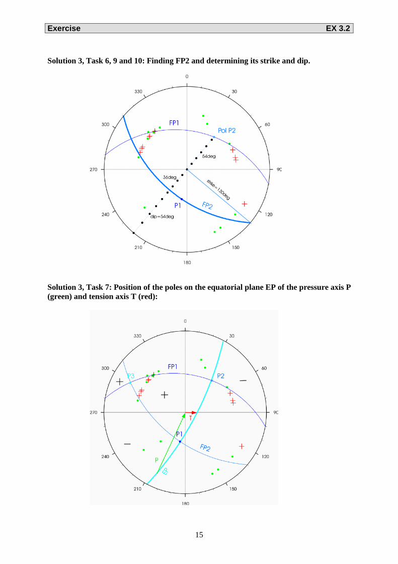
Solutions 4, Tasks 8, 11 and 12: Drawing the slip vectors of FP1 and FP2, determining the rake angle and measuring the azimuth and plunge of the P and T axes. Summary solutions of all tasks: Table 3 summarizes both the angles measured by hand as well as the ones (in brackets) that result from best fitting computer analysis of the polarity plots. The agreement is astonishingly good. Table 3 strike dip rake Fault plane1 (FP1) 280o (278.5°) 40o (39.9°) 68o (67.4°) Fault plane 2 (FP2) 130o (127.0o) 54o (53.7o) 108o (107.8o) azimuth plunge Pressure axis 205o (204.4o) 7o (7.1o) Tension axis 90o (88.6o) 73o (74.0o) Solution 5, Task 14: a) FP2 was more likely the active fault. b) The aftershock was a thrust event with a very small right-lateral strike-slip component.

Exercise EX 3.2

17

c) The slip direction is here strike - rake azimuth, i.e., for FP2 130° - 108° = 12° from north. This is close to the direction of maximum horizontal compression (15°) in the nearby area as derived from centroid moment-tensor solutions of stronger events.

d) The strike of FP2 for this event agrees quite well with the strike direction of mapped local

faults F1, F2, and F3 in the horse tail formed aftershock cloud southeast of the Erzincan basin. The strongest aftershock (Ms = 5.8) on March 15, 1992 (small double circles) took place in the horse tail part, too. Therefore, it is probable that FP2 was the acting fault. The North Anatolian Fault (NAF) which reflects the general tectonics confines the northern margin of the aftershock zone and it is continuing towards the triple point of the NAF with the East Anatolian Fault.

Reference Grosser, H, Baumbach, M., Berckhemer, H., Baier, B., Karahan, A., Schelle, H., Krüger, F.,

Paulat, A., Michel, G., Demirtas, R., Gencoglu, S., and Yilmaz, R. (1998). The Erzincan (Turkey) Earthquake (Ms 6.8) of March 13, 1992 and its Aftershock Sequence. Pure appl. Geophys., 152, 465–505.

Acknowledgment The authors are grateful to Dr. Helmut Grosser for his careful review and useful comments which helped to improve the manuscript and for providing us with a figure of Grosser et al. (1998) to be amended for the purpose of this exercise.