Topic 5

R&D and Patent Law

5.1 Classifications of Process Innovation

• classifies process (cost-reducing) innovation according to the magnitude of the cost reduction gener-ated by the R&D process.

• industry producing a homogeneous product

• firms compete in prices.

• initially, all firms possess identical technologies: with a unit production cost c0 > 0.

-

6llllllllllllllll

TTTTTTTTTTTTTT

Q

p

c0

c2

c1

pm(c1)

pm(c2)

p1 = p0

MR(Q)

D

Q1 Q0 Q2

•

•

Figure 5.1: Classification of process innovation

Definition 5.1Let pm(c) denote the price that would be charged by a monopoly firm whose unit production cost isgiven by c. Then,(a) Innovation is said to be large (or drastic, or major) if

pm(c) < c0. That is, if innovation reduces the cost to a level where the associated pure monopolyprice is lower than the unit production costs of the competing firms.

(b) Innovation is said to be small (or nondrastic, or minor) ifpm(c) > c0.

(Downloaded from www.ozshy.com) (draft=gradio21.tex 2007/12/11 12:19)

5.2 Innovation Race 31

Example: Consider the linear inverse demand function p = a − bQ. Then, innovation is major ifc1 < 2c0 − a and minor otherwise.

5.2 Innovation Race

Two types of models:

Memoryless: Probability of discovery is independent of experience (thus, depends only on current R&Dexpenditure).

Cumulating Experience: Probability of discovery increases with cumulative R&D experience (like capitalstock).

5.2.1 Memoryless model

Lee and Wilde (1980), Loury (1979), and Reinganum. The model below is Exercise 10.5, page 396 inTirole.

• n firms race for a prize V (present value of discounted benefits from getting the patent)

• each firm is indexed by i, i = 1, 2, . . . , n

• xi ≥ 0 is a commitment to a stream of R&D investment (at any t, t ∈ [0,∞)).

• h(xi) is probability that firm i discovers the at ∆t when it invests xi in this time interval, whereh′ > 0, h′′ < 0, h(0) = 0, h′(0) =∞, h′(+∞) = 0

• τi date firm i discovers (random variable)

• τ̂idef= minj 6=i{τj(xj)} date in which first rival firm discovers (random variable).

Probability that firm i discovers before or at t is

Pr(τi(xi) ≤ t) = 1− e−h(xi)t, density is: h(xi)e−h(xi)t

Probability that firm i does not discover by t

Pr(τi(xi) > t) = e−h(xi)t

Probability that all n firms do NOT discover before t

Pr(τ̂i ≤ t) = 1− Pr{τj > t ∀i} = 1−(

1− e−∑ni=1 h(xi)t

)= e−

∑ni=1 h(xi)t

Define aidef=∑

j 6=i hj(xj).Remark : Probability at least one rival discovers before t

Pr(τ̂i ≤ t) = 1− Pr{τj > t ∀j 6= i} = 1− e−ait

The expected value of firm i is

Vi =

∞∫0

e−rte−t∑ni=1 h(xi) [h(xi)V − xi] dt =

h(xi)V − xir + ai + h(xi)

(Downloaded from www.ozshy.com) (draft=gradio21.tex 2007/12/11 12:19)

5.2 Innovation Race 32

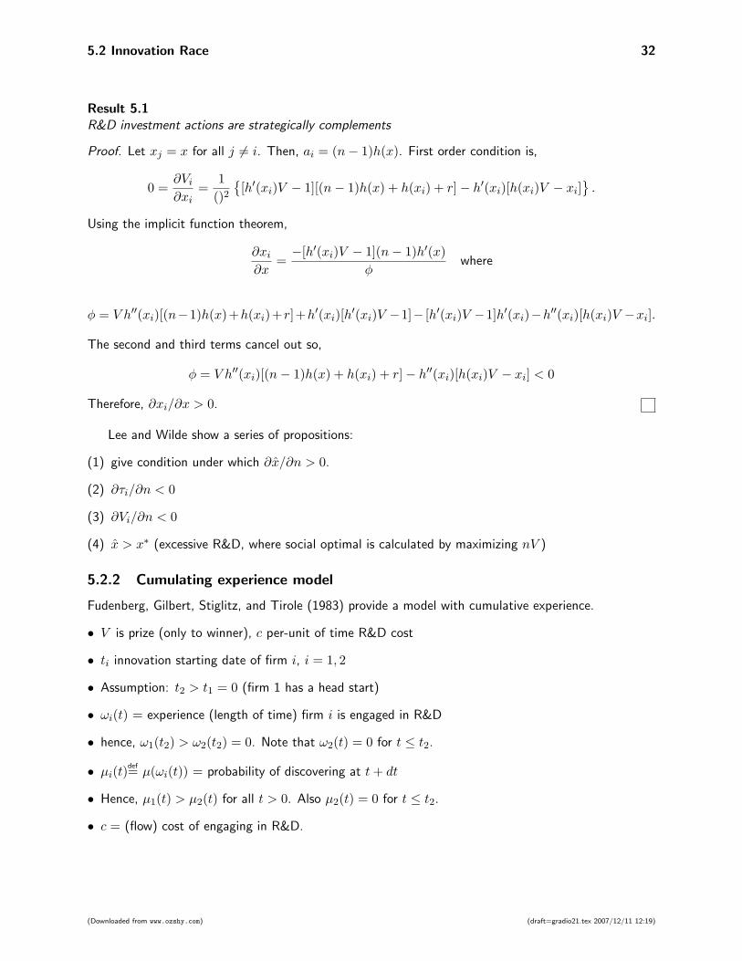
Result 5.1R&D investment actions are strategically complements

Proof. Let xj = x for all j 6= i. Then, ai = (n− 1)h(x). First order condition is,

0 =∂Vi∂xi

=1

()2

{[h′(xi)V − 1][(n− 1)h(x) + h(xi) + r]− h′(xi)[h(xi)V − xi]

}.

Using the implicit function theorem,

∂xi∂x

=−[h′(xi)V − 1](n− 1)h′(x)

φwhere

φ = V h′′(xi)[(n−1)h(x)+h(xi)+r]+h′(xi)[h′(xi)V −1]− [h′(xi)V −1]h′(xi)−h′′(xi)[h(xi)V −xi].

The second and third terms cancel out so,

φ = V h′′(xi)[(n− 1)h(x) + h(xi) + r]− h′′(xi)[h(xi)V − xi] < 0

Therefore, ∂xi/∂x > 0.

Lee and Wilde show a series of propositions:

(1) give condition under which ∂x̂/∂n > 0.

(2) ∂τi/∂n < 0

(3) ∂Vi/∂n < 0

(4) x̂ > x∗ (excessive R&D, where social optimal is calculated by maximizing nV )

5.2.2 Cumulating experience model

Fudenberg, Gilbert, Stiglitz, and Tirole (1983) provide a model with cumulative experience.

• V is prize (only to winner), c per-unit of time R&D cost

• ti innovation starting date of firm i, i = 1, 2

• Assumption: t2 > t1 = 0 (firm 1 has a head start)

• ωi(t) = experience (length of time) firm i is engaged in R&D

• hence, ω1(t2) > ω2(t2) = 0. Note that ω2(t) = 0 for t ≤ t2.

• µi(t)def= µ(ωi(t)) = probability of discovering at t+ dt

• Hence, µ1(t) > µ2(t) for all t > 0. Also µ2(t) = 0 for t ≤ t2.

• c = (flow) cost of engaging in R&D.

(Downloaded from www.ozshy.com) (draft=gradio21.tex 2007/12/11 12:19)

5.2 Innovation Race 33

Expected instantaneous profit conditional that no firm having yet made the discovery is

µi(t)V − c

Probability that neither firm makes the discovery before t

e−∫ t0 [µ1(ω1(τ))+µ2(ω2(τ))]dτ

When both firms undertake R&D, from t1 and t2, respectively,

Vi =

∞∫ti

e−[rt+∫ t0 [µ1(ω1(τ))+µ2(ω2(τ))]dτ ] [µi(ωi(t))V − c] dt

Assumptions:

(1) R&D is potentially profitable for the monopolist. Formally, there exists ω̄ > 0 such that µ(ω)V −c >0 for all ω > ω̄; and µ(0)V − c < 0.

(2) R&D is profitable for a monopolist. Formally,

∞∫0

e−[rt+∫ t0 [µ(τ)]dτ ] [µ(t)V − c] dt > 0.

(3) R&D is unprofitable for a firm in a duopoly. Formally,

∞∫0

e−[rt+∫ t0 [2µ(τ)]dτ ] [µ(t)V − c] dt < 0.

-

6

ω2

ω1

V2 > 0

V2 < 0

V1 < 0actual path

k

t2

45◦

V2(ω1, ω2) = 0

V2(ω1, ω2) = 0

Firm 1 stays in

Firm 2 stays in

Both stay in

Figure 5.2: Locuses of Vi(ω1(τ), ω2(τ)) = 0, i = 1, 2 (note: t2 > t1 = 0)

(Downloaded from www.ozshy.com) (draft=gradio21.tex 2007/12/11 12:19)

5.3 R&D Joint Ventures 34

Results:

(1) ε-preemption. That is, firm 2 does not enter the race.

(2) if we add another stage of uncertainty (associated with developing the innovation), leapfrogging ispossible and there is no ε-preemption

5.3 R&D Joint Ventures

Many papers (see Choi 1993; d’Aspremont and Jacquemin 1988; Kamien, Muller, and Zang 1992; Katz1986, and Katz and Ordover 1990).

• two-stage game: at t = 1, firms determine (first noncooperatively and then cooperatively) how muchto invest in cost-reducing R&D and, at t = 2, the firms are engaged in a Cournot quantity game

• market for a homogeneous product, aggregate demand p = 100−Q.

• xi the amount of R&D undertaken by firm i,

• ci(x1, x2) the unit production cost of firm i

ci(x1, x2)def= 50− xi − βxj i 6= j, i = 1, 2, β ≥ 0.

Definition 5.2We say that R&D technologies exhibit (positive) spillover effects if β > 0.

Assumption 5.1Research labs operate under decreasing returns to scale. Formally,

TCi(xi) =(xi)2

2.

We analyze 2 (out of 3) market structures:

(1) Noncoordination: Look for a Nash equilibrium in R&D efforts: x1 and x2.

(2) Coordination (semicollusion): Determine each firm’s R&D level, x1 and x2 as to maximize jointprofit, while still maintaining separate labs.

(3) R&D Joint Venture (RJV semicollusion): Setting a single lap. The present model does not fit thismarket structure.

5.3.1 Noncooperative R&D

The second period

πi(c1, c2)|t=2 =(100− 2ci + cj)2

9for i = 1, 2, i 6= j. (5.1)

(Downloaded from www.ozshy.com) (draft=gradio21.tex 2007/12/11 12:19)

5.3 R&D Joint Ventures 35

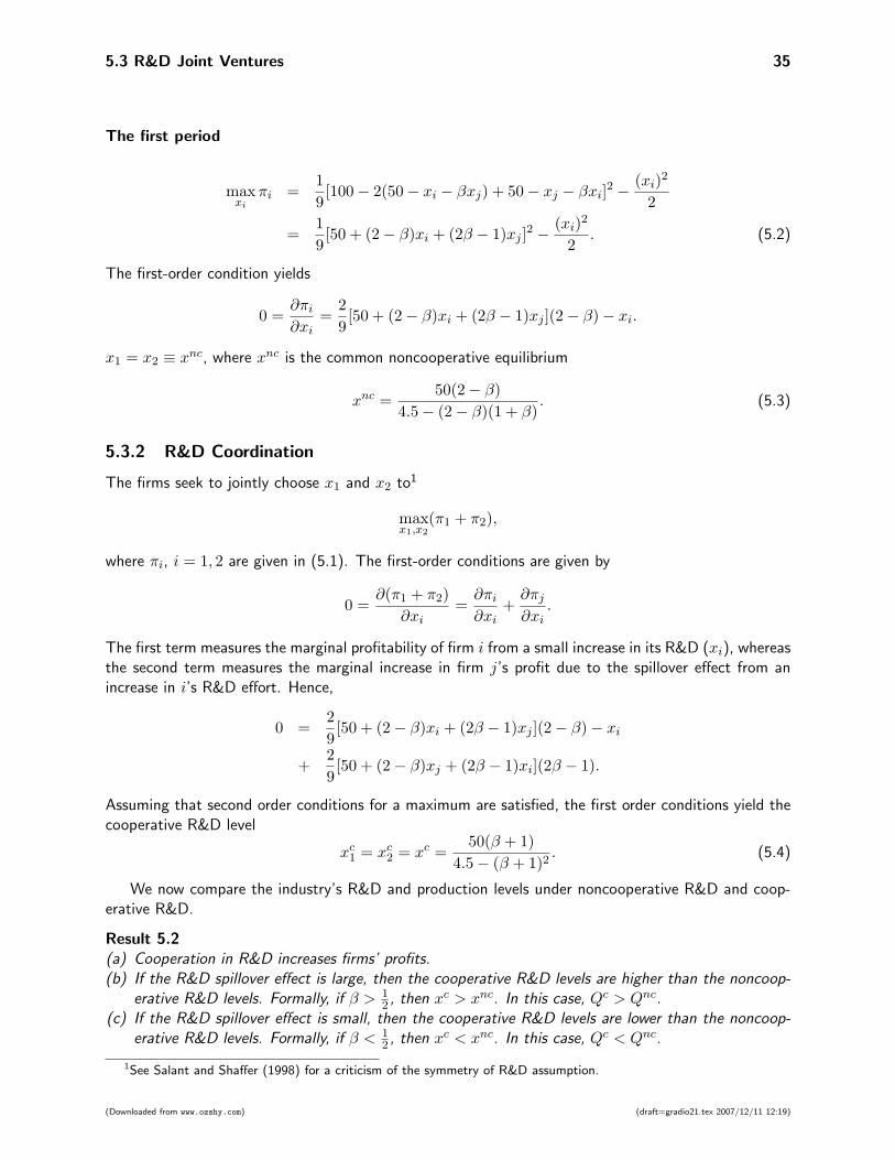
The first period

maxxi

πi =19

[100− 2(50− xi − βxj) + 50− xj − βxi]2 −(xi)2

2

=19

[50 + (2− β)xi + (2β − 1)xj ]2 −(xi)2

2. (5.2)

The first-order condition yields

0 =∂πi∂xi

=29

[50 + (2− β)xi + (2β − 1)xj ](2− β)− xi.

x1 = x2 ≡ xnc, where xnc is the common noncooperative equilibrium

xnc =50(2− β)

4.5− (2− β)(1 + β). (5.3)

5.3.2 R&D Coordination

The firms seek to jointly choose x1 and x2 to1

maxx1,x2

(π1 + π2),

where πi, i = 1, 2 are given in (5.1). The first-order conditions are given by

0 =∂(π1 + π2)

∂xi=∂πi∂xi

+∂πj∂xi

.

The first term measures the marginal profitability of firm i from a small increase in its R&D (xi), whereasthe second term measures the marginal increase in firm j’s profit due to the spillover effect from anincrease in i’s R&D effort. Hence,

0 =29

[50 + (2− β)xi + (2β − 1)xj ](2− β)− xi

+29

[50 + (2− β)xj + (2β − 1)xi](2β − 1).

Assuming that second order conditions for a maximum are satisfied, the first order conditions yield thecooperative R&D level

xc1 = xc2 = xc =50(β + 1)

4.5− (β + 1)2. (5.4)

We now compare the industry’s R&D and production levels under noncooperative R&D and coop-erative R&D.

Result 5.2(a) Cooperation in R&D increases firms’ profits.(b) If the R&D spillover effect is large, then the cooperative R&D levels are higher than the noncoop-

erative R&D levels. Formally, if β > 12 , then xc > xnc. In this case, Qc > Qnc.

(c) If the R&D spillover effect is small, then the cooperative R&D levels are lower than the noncoop-erative R&D levels. Formally, if β < 1

2 , then xc < xnc. In this case, Qc < Qnc.

1See Salant and Shaffer (1998) for a criticism of the symmetry of R&D assumption.

(Downloaded from www.ozshy.com) (draft=gradio21.tex 2007/12/11 12:19)

5.4 Patents 36

5.4 Patents

• We search for the socially optimal patent life T (is it 17 years?)

• Process innovation reduces the unit cost of the innovating firm by x

• For simplicity, we restrict our analysis to minor innovations only.

• market demand given by p = a−Q, where a > c.

-

6

ccccccccccccc

M DL

c

c− x

a− c a− (c− x) aQ

p

a

Figure 5.3: Gains and losses due to patent protection (assuming minor innovation)

M(x) = (a− c)x and DL(x) =x2

2. (5.5)

5.4.1 Innovator’s choice of R&D level for a given duration of patents

Denote by π(x;T ) the innovator’s present value of profits when the innovator chooses an R&D levelof x. Then, in the second stage the innovator takes the duration of patents T as given and chooses inperiod t = 1 R&D level x to

maxx

π(x;T ) =T∑t=1

ρt−1M(x)− TC(x). (5.6)

That is, the innovator chooses R&D level x to maximize the present value of T years of earning monopolyprofits minus the cost of R&D. We need the following Lemma.

Lemma 5.1

T∑t=1

ρt−1 =1− ρT

1− ρ.

(Downloaded from www.ozshy.com) (draft=gradio21.tex 2007/12/11 12:19)

5.4 Patents 37

Proof.

T∑t=1

ρt−1 =T−1∑t=0

ρt =1

1− ρ− ρT − ρT+1 − ρT+2 − . . .

=1

1− ρ− ρT (1 + ρ+ ρ2 + ρ3 + . . .)

=1

1− ρ− ρT

1− ρ=

1− ρT

1− ρ.

Hence, by Lemma 5.1 and (5.5), (5.6) can be written as

maxx

1− ρT

1− ρ(a− c)x− x2

2,

implying that the innovator’s optimal R&D level is

xI =1− ρT

1− ρ(a− c). (5.7)

Hence,

Result 5.3(a) The R&D level increases with the duration of the patent. Formally, xI increases with T .(b) The R&D level increases with an increase in the demand, and decreases with an increase in the unit

cost. Formally, xI increases with an increase in a and decreases with an increase in c.(c) The R&D level increases with an increase in the discount factor ρ (or a decrease in the interest

rate).

5.4.2 Society’s optimal duration of patents

Formally, the social planner calculates profit-maximizing R&D (5.7) for the innovator, and in periodt = 1 chooses an optimal patent duration T to

maxT

W (T ) ≡∞∑t=1

ρt−1[CS0 +M(xI)

]+

∞∑t=T+1

ρt−1DL(xI)− (xI)2

2

s.t. xI =1− ρT

1− ρ(a− c). (5.8)

Since∞∑

t=T+1

ρt−1 = ρT∞∑t=0

ρt =ρT

1− ρ

and using (5.5), (5.8) can be written as choosing T ∗ to maximize

W (T ) =CS0 + (a− c)xI

1− ρ− (xI)2

21− ρ− ρT

1− ρs.t. xI =

1− ρT

1− ρ(a− c). (5.9)

Thus, the government acts as a leader since the innovator moves after the government sets the patentlength T , and the government moves first and chooses T knowing how the innovator is going to respond.

(Downloaded from www.ozshy.com) (draft=gradio21.tex 2007/12/11 12:19)

5.5 Appropriable Rents from Innovation in the Absence of Property Rights 38

We denote by T ∗ the society’s optimal duration of patents. We are not going to actually performthis maximization problem in order to find T ∗. In general, computer simulations can be used to find thewelfare-maximizing T in case differentiation does not lead to an explicit solution, or when the discretenature of the problem (i.e., T is a natural number) does not allow us to differentiate at all. However,one conclusion is easy to find:

Result 5.4The optimal patent life is finite. Formally, T ∗ <∞.

Proof. It is sufficient to show that the welfare level under a one-period patent protection (T = 1)exceeds the welfare level under the infinite patent life (T =∞). The proof is divided into two parts forthe cases where ρ < 0.5 and ρ ≥ 0.5.

First, for ρ < 0.5 when T = 1, xI(1) = a− c. Hence, by (5.9),

W (1) =CS0 + (a− c)2

1− ρ− (a− c)2

21− 2ρ1− ρ

=CS0

1− ρ+

(a− c)2

1− ρ1 + 2ρ

2. (5.10)

When T = +∞, xI(+∞) = a−c1−ρ . Hence, by (5.9),

W (+∞) =CS0

1− ρ+

(a− c)2

(1− ρ)2− (a− c)2

2(1− ρ)2=

CS0

1− ρ+

(a− c)2

2(1− ρ)2. (5.11)

A comparison of (5.10) with (5.11) yields that

W (1) > W (∞)⇐⇒ (a− c)2

1− ρ1 + 2ρ

2>

(a− c)2

2(1− ρ)2⇐⇒ ρ < 0.5. (5.12)

Second, for ρ ≥ 0.5 we approximate T as a continuous variable. Differentiating (5.9) with respectto T and equating to zero yields

T ∗ =ln[3 +

√6 + ρ2 − 6ρ− ρ]− ln(3)

ln(ρ)<∞.

Now, instead of verifying the second-order condition, observe that for T = 1, dW (1)/dT = [(a −c)2ρ(1− 5ρ) ln(ρ)]/[2(1− ρ)2] > 0 for ρ > 0.2.

5.5 Appropriable Rents from Innovation in the Absence of Property Rights

Following Anton an Yao (AER, 1994), we show that

• Even without patent law, a non-reproducible innovation can provide with a substantial amount ofprofit.

• This holds true also for innovators with no assets (poor innovators).

The model

• One innovator, financially broke

• πM profit level if only one firm gets the innovation

• πD profit level to each firm if two firms get the innovation

(Downloaded from www.ozshy.com) (draft=gradio21.tex 2007/12/11 12:19)

5.5 Appropriable Rents from Innovation in the Absence of Property Rights 39

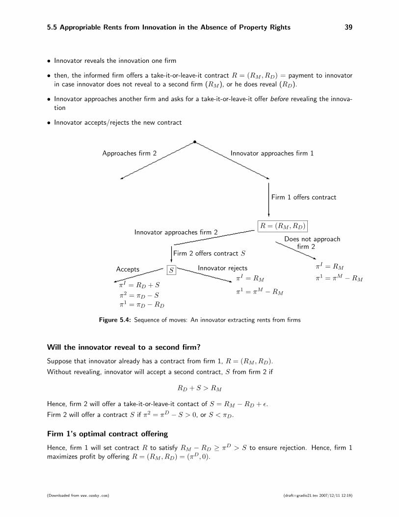
• Innovator reveals the innovation one firm

• then, the informed firm offers a take-it-or-leave-it contract R = (RM , RD) = payment to innovatorin case innovator does not reveal to a second firm (RM ), or he does reveal (RD).

• Innovator approaches another firm and asks for a take-it-or-leave-it offer before revealing the innova-tion

• Innovator accepts/rejects the new contract

j�

•Innovator approaches firm 1Approaches firm 2

?

Firm 1 offers contract

R = (RM , RD)

j

Does not approachfirm 2

Innovator approaches firm 2

?Firm 2 offers contract S

SπI = RM

π1 = πM −RMz πI = RM

π1 = πM −RM

Innovator rejects

9

Accepts

πI = RD + S

π2 = πD − Sπ1 = πD −RD

Figure 5.4: Sequence of moves: An innovator extracting rents from firms

Will the innovator reveal to a second firm?

Suppose that innovator already has a contract from firm 1, R = (RM , RD).

Without revealing, innovator will accept a second contract, S from firm 2 if

RD + S > RM

Hence, firm 2 will offer a take-it-or-leave-it contact of S = RM −RD + ε.

Firm 2 will offer a contract S if π2 = πD − S > 0, or S < πD.

Firm 1’s optimal contract offering

Hence, firm 1 will set contract R to satisfy RM − RD ≥ πD > S to ensure rejection. Hence, firm 1maximizes profit by offering R = (RM , RD) = (πD, 0).

(Downloaded from www.ozshy.com) (draft=gradio21.tex 2007/12/11 12:19)