Top Wealth Shares in the United States, 1916-2000:

Evidence from Estate Tax Returns

Wojciech Kopczuk, Columbia University and NBER

and

Emmanuel Saez, UC Berkeley and NBER1 2.

March 15, 2004

1Wojciech Kopczuk, Department of Economics and SIPA, Columbia University, 420 West 118th Street,

Rm. 1022 IAB MC 3308, New York, NY 10027, wkopczuk@nber.org. Emmanuel Saez, University of Cal-

ifornia, Department of Economics, 549 Evans Hall #3880, Berkeley, CA 94720, saez@econ.berkeley.edu.

We are extremely grateful to Barry Johnson for facilitating our use of the micro estate tax returns data

and for his enormous help and patience explaining it. We thank Ed Wolff for providing us with additional

and unpublished data from Wolff (1989). We thank two anonymous referees, Tony Atkinson, Alan Auer-

bach, David Joulfaian, Arthur Kennickell, Thomas Piketty, Karl Scholz, James Poterba, Joel Slemrod,

Scott Weisbenner, and numerous seminar participants for very helpful comments and discussions. Jeff

Liebman and Jeff Brown kindly shared their socioeconomic mortality differential measures. Financial

support from NSF Grant SES-0134946 and from the Social Sciences and Humanities Research Council

of Canada is gratefully acknowledged.2Complete details about methodology and results are available in the NBER Working Paper version,

Kopczuk and Saez (2004)

Abstract

This paper presents new homogeneous series on top wealth shares from 1916 to 2000 in the

United States using estate tax return data. Top wealth shares were very high at the beginning

of the period but have been hit sharply by the Great Depression, the New Deal, and World

War II shocks. Those shocks have had permanent effects. Following a decline in the 1970s, top

wealth shares recovered in the early 1980s, but they are still much lower in 2000 than in the early

decades of the century. Most of the changes we document are concentrated among the very top

wealth holders with much smaller movements for groups below the top 0.1%. Consistent with

the Survey of Consumer Finances results, top wealth shares estimated from Estate Tax Returns

display no significant increase since 1995. Evidence from the Forbes 400 richest Americans

suggests that only the super-rich have experienced significant gains relative to the average over

the last decade. Our results are consistent with the decreased importance of capital income at

the top of the income distribution documented by Piketty and Saez (2003), and suggest that the

rentier class of the early century is not yet reconstituted. The paper proposes several tentative

explanations to account for the facts.

1 Introduction

The pattern of wealth and income inequality during the process of development of modern

economies has attracted enormous attention since Kuznets (1955) formulated his famous in-

verted U-curve hypothesis. Wealth tends to be much more concentrated than income because

of life cycle savings and because it can be transmitted from generation to generation. Liberals

have blamed wealth concentration because of concerns for equity and in particular for tilting

the political process in the favor of the wealthy. They have proposed progressive taxation as

an appropriate counter-force against wealth concentration.1 For conservatives, concentration of

wealth is considered as a natural and necessary outcome of an environment that provides incen-

tives for entrepreneurship and wealth accumulation, key elements of macro-economic success.

Redistribution through progressive taxation might weaken those incentives and generate large

efficiency costs. Therefore, it is of great importance to understand the forces driving wealth

concentration over time and whether government interventions through taxation or other regu-

lations are effective and/or harmful to curb wealth inequality. This task is greatly facilitated by

the availability of long and homogeneous series of income or wealth concentration. Such series

are in general difficult to construct because of lack of good data. In this paper, we use the ex-

traordinary micro dataset of estate tax returns that has been recently compiled by the Statistics

of Income Division of the Internal Revenue Service (IRS) in order to construct homogeneous

series of wealth shares accruing to the upper groups of the wealth distribution since 1916, the

beginning of the modern federal estate tax in the United States.

The IRS dataset includes detailed micro-information for all federal estate tax returns filed

during the 1916-1945 period.2 We supplement these data with both published tabulations and

other IRS micro-data of estate tax returns from selected years of the second half of the century.

We use the estate multiplier technique, which amounts to weighting each estate tax return by the

inverse probability of death, to estimate the wealth distribution of the living adult population

from estate data. First, we have constructed almost annual series of shares of total wealth1In the early 1930s, President Roosevelt justified the implementation of drastic increases in the burden and

progressivity of federal income and estate taxation in large part on those grounds.2The estate tax return data was compiled electronically and hence saved for research purposes thanks to Fritz

Scheuren, former director of the Statistics of Income division at the IRS.

1

accruing to various sub-groups within the 2% of the wealth distribution.3 Although small in

size, these top groups hold a substantial fraction of total net worth in the economy. Second,

for each of these groups, we decompose wealth into various sources such as real estate, fixed

claims assets (bonds, cash, mortgages, etc.), corporate stock, and debts. We also display the

composition by gender, age, and marital characteristics. This exercise follows in the tradition

of Lampman (1962), who produced top wealth share estimates for a few years between 1922

and 1956. Lampman, however, did not analyze groups smaller than the top .5% and this is

an important difference because our analysis shows that, even within the top percentile, there

is dramatic heterogeneity in the shares of wealth patterns. Most importantly, nobody has

attempted to estimate, as we do here, homogeneous series covering the entire century.4

Our series show that there has been a sharp reduction in wealth concentration over the 20th

century: the top 1% wealth share was close to 40% in the early decades of the century but has

fluctuated between 20 and 25% over the last three decades. This dramatic decline took place at

a very specific time period, from the onset of Great Depression to the end of World War II, and

was concentrated in the very top groups within the top percentile, namely groups within the

top 0.1%. Changes in the top percentile below the top 0.1% have been much more modest. It is

fairly easy to understand why the shocks of the Great Depression, the New Deal policies which

increased dramatically the burden of estate and income taxation for the wealthy, and World

War II, could have had such a dramatic impact on wealth concentration. However, top wealth

shares did not recover in the following decades, a period of rapid growth and great economic

prosperity. In the early 1980s, top wealth shares have increased, and this increase has also been

very concentrated. However, this increase is small relative to the losses from the first part of

the twentieth century and the top wealth shares increased only to the levels prevailing prior to

the recessions of the 1970s. Furthermore, this increase took place in the early 1980s and top

shares were stable during the 1990s. This evidence is consistent with the dramatic decline in top3For the period 1916-1945, because of very high estate tax exemption levels, the largest group we can consider

is the top 1%.4Smith (1984) provides estimates for some years between 1958 and 1976 but his series are not fully consistent

with Lampman (1962). Wolff (1994) has patched series from those authors and non-estate data sources to produce

long-term series. We explain in detail in Section 5.3 why such a patching methodology can produce misleading

results.

2

capital incomes documented in Piketty and Saez (2003) using income tax return data. As they

do, we tentatively suggest (but do not prove) that steep progressive income and estate taxation,

by reducing the rate of wealth accumulation of the rich, may have been the most important

factor preventing large fortunes to be reconstituted after the shocks of the 1929-1945 period.

Perhaps surprisingly, our top wealth shares series do not increase during the 1990s, a time of

the Internet revolution and the creation of dot-com fortunes, extra-ordinary stock price growth,

and of great increase in income concentration (Piketty and Saez, 2003). Our results are never-

theless consistent with findings from the Survey of Consumer Finances (Kennickell, 2003; Scholz,

2003) which also indicate hardly any growth in wealth concentration since 1995. This absence of

growth in top wealth shares in the 1990s is not necessarily inconsistent with the income shares

results from Piketty and Saez (2003) because the dramatic growth in top income shares since

the 1980s has been primarily due to a surge in top labor incomes, with little growth of top

capital incomes. This may suggest that the new high income earners have not had time yet to

accumulate substantial fortunes, either because the pay surge at the top is too recent a phe-

nomenon, or because their savings rates are very low. We show that, as a possible consequence

of democratization of stock ownership in America, the top 1% individuals do not hold today a

significantly larger fraction of their wealth in the form of stocks than the average person in the

U.S. economy, explaining in part why the bull stock market of the late 1990s has not benefited

disproportionately the rich.5

Although there is substantial circumstantial evidence that we find persuasive, we cannot

prove that progressive taxation and stock market democratization had the decisive role we

attribute to them. In our view, the primary contribution of this paper is to provide new and

homogeneous series on wealth concentration using the very rich estate tax statistics. We are

aware that the assumptions needed to obtain unbiased estimates using the estate multiplier

method may not be met and, drawing on previous studies, we try to discuss as carefully as

possible how potential sources of bias, such as estate tax evasion and tax avoidance, can affect

our estimates. Much work is still needed to compare systematically the estate tax estimates5We also examine carefully the evidence from the Forbes 400 richest Americans survey. This evidence shows

sizeable gains but those gains are concentrated among the top individuals in the list and the few years of the

stock market “bubble” of the late 1990s, followed by a sharp decline from 2000 to 2002.

3

with other sources such as capital income from income tax returns, the Survey of Consumer

Finances, and the Forbes 400 list.

The paper is organized as follows. Section 2 describes our data sources and outlines our

estimation methods. Section 3 presents our estimation results. We present and analyze the

trends in top wealth shares and the evolution of the composition of these top wealth holdings.

Section 4 proposes explanations to account for the facts and relates the evolution of top wealth

shares to the evolution of top income shares. Section 5 discusses potential sources of bias, and

compares our wealth share results with previous estimates and estimates from other sources

such as the Survey of Consumer Finances, and the Forbes richest 400 list. Finally, Section 6

offers a brief conclusion. All series and complete technical details about our methodology are

gathered in appendices of the longer NBER working paper version of the paper (Kopczuk and

Saez, 2004).

2 Data, Methodology, and Macro-Series

In this section, we describe briefly the data we use and the broad steps of our estimation method-

ology. Readers interested in the complete details of our methods are referred to the extensive

appendices at the end of the NBER working paper version of the paper. Our estimates are from

estate tax return data compiled by the Internal Revenue Service (IRS) since the beginning of the

modern estate tax in the United States in 1916. In the 1980s, the Statistics of Income division

of the IRS constructed electronic micro-files of all federal estate tax returns filed for individuals

who died in the period 1916 to 1945. Stratified and large electronic micro-files are also available

for 1965, 1969, 1972, 1976, and every year since 1982.6 For a number of years between 1945

and 1965 (when no micro-files are available), the IRS published detailed tabulations of estate

tax returns (U.S. Treasury Department, Internal Revenue Service, various years).7 This paper

uses both the micro-files and the published tabulated data to construct top wealth shares and

composition series for as many years as possible.

In the United States, because of large exemption levels, only a small fraction of decedents

has been required to file estate tax returns. Therefore, by necessity, we must restrict our analysis6Those data are stratified and hence always contain 100% of the very large estates.7Those tabulations are also based on stratified samples with 100% coverage at the top.

4

to the top 2% of the wealth distribution. Before 1946, we can analyze only the top 1%. As

the analysis will show, the top 1%, although a small fraction of the total population, holds

a substantial fraction of total wealth. Further, there is substantial heterogeneity between the

bottom of the top 1% and the very top groups within the top 1%. Therefore, we also analyze in

detail smaller groups within the top 1%: the top .5%, top .25%, the top .1%, the top .05%, and

the top .01%. We also analyze the intermediate groups: top 1-.5% denotes the bottom half of

the top 1%, top .5-.25% denoted the bottom half of the top .5%, etc. Estates represent wealth

at the individual level and not the family or household level. Therefore, it is very important to

note that our top wealth shares are based on individuals and not families. We come back to this

issue later. Each of our top groups is defined relative to the total number of adult individuals

(aged 20 and above) in the U.S. population, estimated from census data. Column (1) of Table 1

reports the number of adult individuals in the United States from 1916 to 2002. The adult

population has more than tripled from about 60 million in 1916 to over 200 million in 2000. In

2000, there were 201.9 million adults and thus the top 1% is defined as the top 2.019 million

wealth holders, etc.

We adopt the well-known estate multiplier method to estimate the top wealth shares for the

living population from estate data. The method consists in inflating each estate observation by

a multiplier equal to the inverse probability of death.8 The probability of death is estimated

from mortality tables by age and gender for each year for the U.S. population multiplied by

a social differential mortality factor to reflect the fact that the wealthy (those who file estate

tax returns) have lower mortality rates than average. The social differential mortality rates

are based on the Brown et al. (2002) differentials between college educated whites relative to

the average population and are assumed constant over the whole period (see Appendix B of

the NBER working paper version for a detailed discussion and analysis of the validity of this

assumption). The estate multiplier methodology will provide unbiased estimates of the wealth

distribution if our multipliers are correct on average and if probability of death is independent

of wealth within each age and gender group for estate tax return filers. This assumption might

not be correct for three main reasons. First, extraordinary expenses such as medical expenses8This method was first proposed in Great Britain almost a century ago by Mallet (1908). Atkinson and

Harrison (1978) describe the method in detail.

5

and loss of labor income may occur and reduce wealth in the years preceding death. Second,

even within the set of estate tax filers, it might be the case that the most able and successful

individuals have lower mortality rates, or inversely that the stress associated with building a

fortune, increases the mortality rate. Last and most importantly, for estate tax avoidance and

other reasons, individuals may start to give away their wealth to relatives as they feel that their

health deteriorates. We will later address each of these very important issues, and try to analyze

whether those potential sources of bias might have changed overtime.

The wealth definition we use is equal to all assets (gross estate) less all liabilities (mortgages,

and other debts) as they appear on estate tax returns. Assets are defined as the sum of tangible

assets (real estate and consumer durables), fixed claim assets (cash, deposits, bonds, mortgages,

etc.), corporate equities, equity in unincorporated businesses (farms, small businesses), and var-

ious miscellaneous assets. It is important to note that wealth reported on estate tax returns only

includes the cash surrender value of pensions. Therefore, future pension wealth in the form of

defined benefits plans, and annuitized wealth with no cash surrender value is excluded. Vested

defined contributions accounts (and in particular 401(k) plans) are included in the wealth defi-

nition. Social Security wealth as well as all future labor income and human wealth is obviously

not included in gross estate. Estate tax returns include the full payout of life insurance but we

include only the cash value of life insurance (i.e., the value of life insurance when the person is

living) in our estimates.

Therefore, we focus on a relatively narrow definition wealth, which includes only the mar-

ketable or accumulated wealth that remains upon the owner’s death. This point is particularly

important for owners of closely held businesses: in many instances, a large part of the value of

their business reflects their personal human capital and future labor, which vanishes at their

death. Both the narrow definition of wealth (on which we focus by necessity because of our

estate data source), and broader wealth definitions including future human wealth are inter-

esting and important to study. The narrow definition is more suited to examine problems of

wealth accumulation and transmission, while the broader definition is more suited to study the

distribution of welfare.9

9The analysis of income distribution captures both labor and capital income and is thus closer to an analysis

of distribution of the broader wealth concept.

6

For the years for which no micro data is available, we use the tabulations by gross estate,

age and gender and apply the estate multiplier method within each cell in order to obtain a

distribution of gross wealth for the living. We then use a simple Pareto interpolation technique

and the composition tables to estimate the thresholds and average wealth levels for each of our

top groups.10 For illustration purposes, Table 2 displays the thresholds, the average wealth level

in each group, along with the number of individuals in each group all for 2000, the latest year

available.

We then estimate shares of wealth by dividing the wealth amounts accruing to each group by

total net-worth of the household sector in the United States. The total net-worth denominator

has been estimated from the Flow of Funds Accounts for the post-war period and from Goldsmith

et al. (1956) and Wolff (1989) for the earlier period.11 The total net-worth denominator includes

all assets less liabilities corresponding to the items reported on estate tax returns so that the

definitions of wealth in the numerator and the denominator are as close as possible. Thus, our

denominator only includes defined contribution pension reserves, and excludes defined benefits

pension reserves. Life insurance reserves, which reflect the cash surrender value of all policies

held are included in our denominator. The total wealth and average wealth (per adult) series

are reported in real 2000 dollars in Columns (3) and (4) of Table 1. The CPI deflator used to

convert current incomes to real incomes is reported in Column (10). The average real wealth

series per adult along with the CPI deflator is plotted in Figure 1. Average real wealth per adult

has increased by a factor of three from 1916 to 2000 but the growth was very uneven during the

period. There was virtually no growth in average real wealth from 1916 to the onset of World

War II. Average wealth then grew steadily from World War II to the late 1960s. Since then,

wealth gross has been slower, except in the 1994-2000 period.12

After we have analyzed the top share data, we will also analyze the composition of wealth10We also use Pareto interpolations to impute values at the bottom of 1% or 2% of the wealth distribution for

years where the coverage of our micro data is not broad enough.11Unfortunately, no annual series exist before 1945. Therefore, we have built upon previous incomplete series

to construct complete annual series for the 1916-1944 period.12It is important to note that comparing real wealth over time is difficult because it requires to use a price

index and there is substantial controversy about how to construct such an index and account properly for the

introduction of new goods. That is why most of the paper focuses on top wealth shares which are independent of

the price index.

7

and the age, gender, and marital status of top wealth holders, for all years where these data

are available. We divide wealth into six categories: 1) real estate, 2) bonds (federal and local,

corporate and foreign) 3) corporate stock, 4) deposits and saving accounts, cash, and notes, 5)

other assets (including mainly equity in non-corporate businesses), 6) all debts and liabilities.

In order to compare the composition of wealth in the top groups with the composition of total

net-worth in the U.S. economy, we display in columns (5) to (9) of Table 1, the fractions of real

estate, fixed claim assets, corporate equity, unincorporated equity, and debts in total net worth

of the household sector in the United States. We also present on Figure 1, the average real value

of corporate equity and the average net worth excluding corporate equity. Those figures show

that the sharp downturns and upturns in average net worth are primarily due to the dramatic

changes in the stock market prices, and that the pattern of net worth excluding corporate equity

has been much smoother.

3 The Evolution of Top Wealth Shares

3.1 Trends

The basic series of top wealth shares are presented in Table 3. Figure 2 displays the wealth

share of the top 1% from 1916 to 2000. The top 1% held close to 40% of total wealth, up to the

onset of the Great Depression. Between 1930 and 1932, the top 1% share fell by more than 10

percentage points, and continued to decline during the New Deal, World War II, and the late

1940s. By 1949, the top 1% share was around 22.5%. The top 1% share increased slightly to

around 25% in the mid-1960s, and then fell to less than 20% in 1976 and 1982. The top 1% share

increases significantly in the early 1980s (from 19% to 22%) and then stays remarkably stable

around 21-22% in the 1990s. This evidence shows that the concentration of wealth ownership in

the United States decreased dramatically over the century. This phenomenon is illustrated on

Figure 3 which displays the average real wealth of those in the top 1% (left-hand-side scale) and

those in the bottom 99% (right-hand-side scale). In 1916, the top 1% wealth holders were more

than 60 times richer on average than the bottom 99%. The figure shows the sharp closing of the

gap between the Great Depression and the post World War II years, as well as the subsequent

parallel growth for the two groups (except for the 1970s). In 2000, the top 1% individuals are

8

about 25 times richer than the rest of the population.

Therefore, the evidence suggests that the twentieth century’s decline in wealth concentration

took place in a very specific and brief time interval, 1930-1949 which spans the Great Depression,

the New Deal, and World War II. This suggests that the main factors influencing the concen-

tration of wealth might be short-term events with long-lasting effects, rather than slow changes

such as technological progress and economic development or demographic transitions.

In order to understand the overall pattern of top income shares, it is useful to decompose

the top percentile into smaller groups. Figure 4 displays the wealth shares of the top 1-.5%

(the bottom half of the top 1%), and the top .5-.1% (the next .4 percentile of the distribution).

Figure 4 also displays the share of the second percentile (Top 2-1%) for the 1946-2000 period.

The figure shows that those groups of high but not super-high wealth holders experienced much

smaller movements than the top 1% as a whole. The top 1-.5% has fluctuated between 5 and 6%

except for a short-lived dip during the Great Depression. The top .5-.1% has experienced a more

substantial and long-lasting drop from 12 to 8% but this 4 percentage point drop constitutes a

relatively small part of the 20 point loss of the top 1%. All three groups have been remarkably

stable over the last 25 years.

Examination of the very top groups in Figure 5 (the top .1% in Panel A and the top .01% in

Panel B) provides a striking contrast to Figure 4. The top .1% declined dramatically from more

than 20% to less than 10% after World War II. For the top .01%, the fall was even more dramatic

from 10% to 4%: those wealthiest individuals, a group of 20,000 persons in 2000, had on average

1000 times the average wealth in 1916, and have about 400 times the average wealth in 2000.

It is interesting to note that, in contrast to the groups below the very top on Figure 4, the fall

for the very top groups continued during World War II. Since the end of World War II, those

top groups have remained fairly stable up to the late 1960s. They experienced an additional

drop in the 1970s, and a very significant increase in the early 1980s: from 1982 to 1985, the top

.01% increased from 2.5% to 4%, a 60% increase. However, as all other groups, those top groups

remained stable in the 1990s. Therefore, the evidence shows that the dramatic movements of

the top 1% share are primarily due to changes taking place within the upper fractiles of the top

1%. The higher the group, the larger the decline. It is thus important to analyze separately

each of the groups within the top 1% in order to understand the difference in the patterns.

9

Popular accounts (see Section 5.3 below) suggest that the computer technology in the recent

decades has created many new rich individuals. Those newly rich individuals are likely to be

much younger than the older rich. However, even if the new rich are younger and hence less likely

to die than the old rich, our estimates based on estate tax data should not be biased downward.

This is because the estate multiplier method corrects for changes in the age distribution of top

wealth holders. Our estimates should, however, become noisier (as the sampling probability by

death is reduced). This phenomenon should generate noisier series in the recent period but with

no systematic bias as long as our multipliers correctly reflect the inverse probability of death

of the wealthy in each age-gender cell.13 However, the series displayed on Figures 2, 4, and 5

are very smooth in the 1990s, suggesting that the groups we consider are large enough so that

sampling variability is small.14

3.2 Composition

Figure 6 displays the composition of wealth within the top 1% for 1929, a year when top wealth

shares and stock prices were very high. Wealth is divided into four components: real estate,

corporate stock (including both publicly traded and closely held stock), fixed claims assets

(all bonds, cash and deposits, notes, etc.), and other assets (including primarily non-corporate

business assets).15 Figure 6 shows that the share of corporate stock is increasing with wealth

while the share of real estate is decreasing with wealth, the share of fixed claims assets being

slightly decreasing (the share of bonds is slightly increasing and the share of cash and deposits

slightly decreasing). In the bottom of the top 0.5%, each of those three component represents

about one third of total wealth. At the very top, stocks represent almost two thirds of total

wealth while real estate constitutes less than 10%. This broad pattern is evident for all the years

of the 1916-2000 period for which we have data:16 the share of stocks increases with wealth and

the share of real estate decreases. The levels, however, may vary over time due mainly to the13If fewer than expected of these young wealthy individuals die, the estimate is downward biased but if more

than expected die, the estimate is upward biased.14The estimates are independent across years as every person dies only once.15Debts have been excluded from the figure but they are reported in Table B3 of the NBER working paper

version.16All these statistics are reported in Table B3 of the NBER working paper version.

10

sharp movements in the stock market.

Figure 7 displays the fraction of corporate stock in net worth over the period 1916-2000 for

the top .5%, and for total net worth in the U.S. economy (from Tables 4 and 1 respectively).

Consistent with Figure 6, the fraction of stock is much higher for the top .5% (around 50%

on average) than for total net worth (around 20% on average). Both series are closely parallel

from the 1920s to the mid 1980s: they peak just before the Great Depression, plunge during the

depression, stay low during the New Deal, World War II, up to the early 1950s, and peak again

in the mid-1960s before plummeting in the early 1980s.

This parallel pattern can explain why the share of wealth held by the top groups dropped so

much during the Great Depression. Real corporate equity held by households fell by 70% from

1929 to 1933 (Figure 1) and the top groups hold a much greater fraction of their wealth in the

form of corporate stock (Figure 7). Those two facts mechanically lead to a dramatic decrease in

the share of wealth accruing to the top groups. The same phenomenon took place in the 1970s

when stock prices plummeted and the shares of top groups declined substantially (the real price

of corporate stock fell by 60% and the top 1% fell by about 20% from 1965 to 1982).

Corporate profits increased dramatically during World War II, but in order to finance the

war, corporate tax rates increased sharply from about 10% before the war to over 50% during

the war and they stayed at high levels after the war. This fiscal shock in the corporate sector

reduced substantially the share of profits accruing to stock-holders and explains why average

real corporate equity per adult increased by less than 4% from 1941 to 1949 while the average

net worth increased by about 23% (see Figure 1). Thus, top wealth holders, owning mostly

stock, lost relative to the average during the 1940s, and the top shares declined significantly.

The central puzzle to understand is why this explanation does not work in reverse after 1949,

that is, why top wealth shares did not increase significantly from 1949 to 1965 and from 1986

to 2000 when the stock market prices soared, and the fraction of corporate equity in total net

worth of the household sector increased from just around 12% (in 1949 and 1986) to almost 30%

in 1965 and almost 40% in 2000?

The series on wealth composition of top groups might explain the absence of growth in top

wealth shares during the 1986-2000 episode. The fraction of corporate stock in the top groups

did not increase significantly during the period (as can be seen on Figure 7, it actually drops

11

significantly up to 1990 and then recovers during the 1990s). Therefore, although the fraction of

corporate equity in total net worth triples (from 12% to 38%), the fraction of corporate equity

held by the top groups is virtually the same in 1986 and 2000 (as displayed on Figure 7). Thus,

the data imply that the share of all corporate stock from the household sector held by the top

wealth holders fell sharply from 1986 to 2000. Several factors may explain those striking results.

First, the development of defined contribution pensions plans, and in particular 401(k) plans,

and mutual funds certainly increased the number of stock-holders in the American population,17

and thus contributed to the democratization of stock ownership among American families. The

Survey of Consumer Finances shows that the fraction of families holding publicly traded stock

(directly or indirectly through mutual funds and pension plans) has increased significantly in

the last two decades, and was just above 50% in 2001.18

Second, the wealthy may have re-balanced their portfolios as gains from the stock-market

were accruing in the late 1980s and the 1990s, and thus reduced their holdings of equity relative

to more modest families.

In any case, the data strikingly suggest that top wealth holders did not benefit dispropor-

tionately from the bull stock market relative to the average wealth holder.19 This might explain

in part why top wealth shares did not increase in that period when top income shares were

dramatically increasing (see Section 5 below). By the year 2000, the fraction of wealth held

in stock by the top 1% is just slightly above the fraction of wealth held in stock by the U.S.

household sector (40% versus 38%). Therefore, in the current period, sharp movements of the

stock market are no longer expected to produce sharp movements in top wealth shares as was

the case in the past.20

17The Flow of Funds Accounts show that the fraction of corporate stock held indirectly through Defined

Contribution plans and mutual funds doubled from 17% to 33% between 1986 and 2000.18In 1989, only 31.7% of American households owned stock, either directly or indirectly though pension and

mutual funds, while 48.9% and 51.9% did in 1998 and 2001 respectively. See Kennickell et al. (1997) and Aizcorbe

et al. (2003).19It is important to keep in mind that, because the wealth distribution is very skewed, the average wealth is

much larger than median wealth. Obviously, the stock market surge of the 1990s did not benefit the bottom half

of American families who do not hold any stock.20It should be emphasized, though, that the wealthy may not hold the same stocks as the general population.

In particular, the wealthy hold a disproportionate share of closely held stock, while the general population holds

12

3.3 Age, Gender, and Marital Status

Figure 8 displays the average age and the percent female within the top .5% group since 1916.21

The average age displays a remarkable stability over time fluctuating between 55 and 60. Since

the early 1980s, the average age has declined very slightly from 60 to around 57. Thus, the

evidence suggests that there have been no dramatic changes in the age composition of top

wealth holders over time.22 In contrast, the fraction of females among top wealth holders has

almost doubled from around 25% in the early part of the century to around 45% in the 1990s.

The increase started during the Great Depression and continued throughout the 1950s and

1960s, and has been fairly stable since the 1970s. Therefore, there has been substantial gender

equalization in the holding of wealth over the century in the United States, and today, almost

50% of top wealth holders are female. It is striking, comparing Figure 2 and Figure 8, to note

the negative correlation between the top wealth shares and the fraction of women in the top

wealth groups. This suggests that the gender equalization at the top might have contributed to

the decline in top wealth shares measured at the individual level. It is conceivable that wealth

concentration measured at the family level has not declined as much as wealth concentration

measured at the individual level.23

Estate tax law regarding bequests to spouses has changed over time and this might have

affected the gender composition at the top through behavioral responses to estate taxation.

Before 1948, bequests to spouses were not deductible from taxable estates with an exception

of couples located in the so-called community property states where each spouse owned half of

all assets acquired during marriage. Starting in 1948, spousal bequests became deductible up

to 50% of the net estate. In 1981, spousal bequests became fully deductible.24 Those changes

in general only publicly traded stocks through mutual and pension funds (see e.g. Kennickell, 2003). Estate tax

returns statistics separate closely held from publicly traded stock only since 1986.21Those series are reported in Table 4. Series for all other top wealth groups are reported in Table B4 of the

NBER working paper version.22Although, due to significant decreases in mortality over the course of the 20th century, top wealth holders

nowadays have more years of potential lifespan ahead of them and are therefore younger relative to the average

population than in the early part of the century.23We come back to this point in Section 5.3 when we compare our estimates with wealth concentration measures

at the family level obtained with the Survey of Consumer Finances for the recent period.24Similarly, 50% and 100% of spousal gifts became deductible in 1948 and 1981 respectively. In 1976, the

13

might have increased the amount of spousal bequests made by wealthy individuals and hence

potentially increased the fraction of women in the top wealth groups.25 Two points should be

noted.

First, Figure 8 shows that most of increase in female fraction in the top wealth groups

happened before the changes in estate tax law regarding spousal bequests (in 1948 and 1981)

implying that those tax law changes can explain at best a fraction of the trend. As we discuss

below, estate tax rates at the top became very high in the 1930s.26 As a result, in order to

avoid “double estate taxation”, wealthy husbands had an incentive to pass their wealth directly

to the next generations instead of passing it to their widowed spouses. Such a phenomenon

should have decreased the number of wealthy widows, which should have reduced the number of

wealthy widows at the top. Splitting wealth between spouses using gifts before death was not a

better tax strategy as it would have triggered substantial gift taxes (following the introduction

of the gift tax in 1932) before the marital deduction (for estates and gifts) was introduced in

1948. The main reason why the number of women in the top groups increases so much during

the Great Depression seems to be due to differences in wealth composition between genders. In

the late 1920s, wealthy women held a smaller fraction of their wealth in the form of stock than

wealthy men. As a result, wealthy men lost a larger fraction of their wealth following the stock

market crash of 1929 than wealthy women, thereby contributing to the increase in the fraction

of women at the top.

Second, even tax law induced changes in spousal bequests have a real impact on the distribu-

tion of wealth across gender lines, and thus should not necessarily be regarded as unimportant.

The marital status of top wealth holders has experienced relatively modest secular changes.

For males, the fraction of married men has always been high (around 75%), the fraction widowed

has declined slightly (from 10 to 5%) and the fraction single has increased (from 10 to 15%).

For females, the fraction widowed is much higher, although it has declined over the period from

about 40% to 30%. The fraction married has increased from about 40% to 50% for females and

thus the fraction single has been stable around 10%. This reinforces our previous interpretation

marital deduction was modified to allow for the greater of 50% of estate or $250,000 to be deductible.25See Kopczuk and Slemrod (2003) for a detailed discussion of this point.26The top estate rate increased from 20 to 45 percent in 1932, and then to 60% in 1935, to 70% in 1936, and

to 77% in 1941.

14

that the increase in the fraction female at the top of the wealth distribution has not been due

solely to an increase in the number of wealthy widows following increased spousal bequests,

but might reflect increases in female empowerment in the family (fairer distribution of assets

between spouses) and in the labor market (reduction of the income gender gap overtime).

4 Understanding the Patterns

4.1 Are the Results Consistent with Income Inequality Series?

One of the most striking and debated findings of the literature on inequality has been the sharp

increase in income and wage inequality over the last 25 years in the United States (see Katz and

Autor, 1999, for a recent survey). As evidenced from income tax returns, changes have been

especially dramatic at the top end, with large gains accruing to the top income groups (Feenberg

and Poterba, 1993, 2000; Piketty and Saez, 2003). For example, Piketty and Saez (2003) show

that the top 1% income share doubled from 8% in the 1970s to over 16% in 2000.27 How can

we reconcile the dramatic surge in top income shares with the relative stability of top wealth

shares estimated from estate tax data since the 1980s?

Figure 9 casts light on this issue. It displays the top .01% income share from Piketty and

Saez (2003), along with the composition of these top incomes28 into capital income (dividends,

rents, interest income, but excluding capital gains), realized capital gains, business income, and

wages and salaries. Up to the 1980s (and except during World War II), capital income and

capital gains formed the vast majority of the top .01% incomes. Consistently with our top .01%

wealth share series presented on Figure 5B, the top .01% income share was very high in the late

1920s, and dropped precipitously during the Great Depression and World War II, and remained

low until the late 1970s. Thus both the income and the estate tax data suggests the top wealth

holders were hit by the shocks of the Great Depression and World War II and that those shocks

persisted a long time after the war.

Over the last two decades, as can be seen on Figure 9, the top .01% income share has indeed

increased dramatically from 0.9% in 1980 to 3.6% in 2000. However, the important point to27See the series of Piketty and Saez (2003) updated to year 2000.28This group represents the top 13,400 taxpayers in 2000, ranked by income excluding realized capital gains

although capital gains are added back to compute income shares.

15

note is that this recent surge is primarily a wage income phenomenon and to a lesser extent

a business income phenomenon.29 Figure 9 shows that capital income earned by the top .01%

relative to total personal income is not higher in 2000 than it was in the 1970s (around 0.4%).

Adding realized capital gains does not alter this broad picture: capital income including capital

gains earned by the top .01% represents about 1% of total personal income in 2000 versus about

0.75% in the late 1960s, a modest increase relative to the quadrupling of the top .01% income

share during the same period.

Therefore, the income tax data suggest that the dramatic increase in top incomes is a la-

bor income phenomenon that has not translated yet into an increased concentration of capital

income. Therefore, in the recent period as well, the income tax data paints a story that is con-

sistent with our estate tax data findings of stability of the top wealth shares since the mid-1980s.

The pattern of capital income including realized capital gains displayed on Figure 9 is strikingly

parallel to the pattern of the top .01% wealth share of Figure 5B: a mild peak in the late 1960s,

a decline during the bear stock market of the 1970s, a recovery in the early 1980s, and no growth

from 1990 to 2000.

Three elements might explain why the surge in top wages since the 1970s did not lead to

a significant increase in top wealth holdings. First, it takes time to accumulate a large fortune

out of earnings.30 The top .01% average income in the late 1990s is around 10 million dollars

while the top .01% wealth holding is around 60 million dollars. Thus, even with substantial

saving rates, it would take at least a decade to the average top .01% income earner starting

with no fortune to become an average top .01% wealth holder. Second, it is possible that the

savings rates of the recent “working rich” who now form the majority of top income earners,

are substantially lower than the savings rates of the “coupon-clippers” of the early part of the

century. Finally, certain groups of individuals report high incomes on their tax return only

temporarily (e.g., executives who exercise stock-options irregularly, careers of sport or show-29Gains from exercised stock options are reported as wage income on income tax returns. There is no doubt

that the recent explosion in the use of stock options to compensate executives has contributed to the surge in top

wage incomes in the United States.30Even in recent years after the explosion of executive compensation, few of the richest Americans listed on

the annual Forbes 400 survey are salaried executives. Most of them are still either family heirs or successful

entrepreneurs (see Section 5.3.3 below).

16

business stars usually last for just a few years). To the extent that such cases became more

prevalent in recent years (as seems possible based on popular accounts), the sharp increase in

the concentration of annual incomes documented by Piketty and Saez (2003) may translate into

a smaller increase in the concentration of lifetime incomes and accumulated wealth.

The very rough comparison between income and estate data that we have presented suggests

that it would be interesting to try and estimate wealth concentration from income tax return data

using the capitalization of income method. In spite of the existence of extremely detailed and

consistent income tax return annual data in the United States since 1913, this method has very

rarely been used, and the only existing studies have applied the method for isolated years.31 The

explanation for the lack of systematic studies is that the methodology faces serious challenges:

income data provides information only on assets yielding reported income (for example, owner-

occupied real estate or defined contribution pension plans could not be observed), and there is

substantial and unobservable heterogeneity in the returns of many assets, especially corporate

stock (for example, some corporations rarely pay dividends and capital gains are only observed

when realized on income tax returns).32 More recently, Kennickell (2001a,b) has analyzed in

detail the link between income and wealth in order to calibrate sample weights for the Survey

of Consumer Finances. His analysis shows that the relation between capital income reported on

tax returns and wealth from the survey is extremely noisy at the individual level. Nevertheless,

it would certainly be interesting to use income tax return data to provide a tighter comparison

with our wealth concentration results from estates. We leave this important and ambitious

project for future research.

4.2 Possible Explanations for the Decline in Top Wealth Shares

We have described in the previous section the dramatic fall in the top wealth shares (concentrated

within the very top groups) that has taken place from the onset of the Great Depression to the

late 1940s. Our previous analysis has shown that stock market effects might explain the sharp31King (1927) and Stewart (1939) used this method for years 1921 and 1922-1936 respectively. More recently,

Greenwood (1983) has constructed wealth distributions for 1973 using simultaneously income tax return data and

other sources.32See Atkinson and Harrison (1978) for a detailed comparison of the income capitalization and the estate

multiplier methods for the United Kingdom.

17

drop in top wealth shares during the 1930s but cannot explain the absence of recovery in top

wealth shares in the 1950s and 1960s once stock prices recovered by the end of the 1960s. At

that time, the wealth composition in top groups was again very similar to what it had been in

the late 1920s, and yet top wealth shares hardly recovered in the 1950s and 1960s and were still

much lower in the 1960s than before the Great Depression. There are several possible elements

that might explain the absence of recovery of top wealth shares.

The first and perhaps most obvious factor is the creation and the development of the pro-

gressive income and estate tax. The very large fortunes (such as the top .01%) observed at

the beginning of the 20th century were accumulated during the 19th century, at a time where

progressive taxes hardly existed and capitalists could dispose of almost 100% of their income

to consume, accumulate, and transmit wealth across generations. The conditions faced by 20th

century fortunes after the shock of the Great Depression were substantially different. Starting in

1933 with the new Roosevelt administration, and continuously until the Reagan administrations

of 1980s, top tax rates on both income and estates have been set at very high levels.

These very high marginal rates applied only to a very small fraction of taxpayers and estates,

but the point is that they were to a large extent designed to hit incomes and estates of the top

0.1% and 0.01% of the distribution. In the presence of progressive capital income taxation,

individuals with large wealth levels need to increase their savings rates out of after tax income

much more than lower wealth holders to maintain their relative wealth position. Moreover,

reduced after-tax rate of return might have affected savings rates of high wealth holders through

standard incentive effects. In the presence of high income and estate taxes, wealthy individuals

also have incentives to give more to charities during their lifetime further reducing top wealth

shares.33

Second, starting with Sherman and Clayton Acts enacted in 1890 and 1914 respectively,

the U.S. federal government has taken important steps to limit monopoly power using antitrust

regulation. However, the degree of enforcement remained weak until the New Deal (see e.g.,

Thorelli, 1955). By curbing the power of monopolies, it is conceivable that such legislation

contributed to reduced wealth concentration at the very top. Perhaps more importantly, the33Lampman (1962) also favored progressive taxation as one important factor explaining the reduction in top

wealth shares in his seminal study (see below).

18

Roosevelt administration also introduced legislation to sever the link between finance and man-

agement of corporations. The Depression’s financial market reforms act broke the links between

board membership, investment banking, and commercial banking. As a result, the model of

great financiers-industrialists which had created the very large fortunes of the Robber Barons

of the late nineteenth and early twentieth century was no longer a possibility after the 1930s.

DeLong (2002) discusses those aspects in more detail and suggests that such regulations severely

prevented the creation of new billionaires during the very prosperous post-World War II decades.

Finally, the post World War II decades were characterized by a large democratization of

higher education. Following the G.I. bill, the number of college educated men increased very

quickly after World War II.34 This undoubtedly contributed to the emergence of a large middle

and upper middle income class in America which was able to accumulate wealth and hence

perhaps reduce the share of total wealth accruing to the groups in the top percentile.35

Although we cannot observe the counterfactual world without progressive taxation or an-

titrust regulations, we note that economic growth, in net worth and incomes, has been much

stronger starting with World War II, than in the earlier period. Thus, the macro-economic

evidence does not suggest that progressive taxation prevented the American capital stock from

recovering from the shock of the Great Depression. This is consistent with Piketty (2003), who

shows that, in the purest neo-classical model without any uncertainty, a capital income tax

affecting only the rich does not affect negatively the capital stock in the long-run. If credit

constraints due to asymmetric information are present in the business sector of the economy,

it is even conceivable that redistribution of wealth from large and passive wealth holders to

entrepreneurs with little capital can actually improve economic performance (see e.g., Aghion

and Bolton, 2003, for such a theoretical analysis). Gordon (1998) argues that high personal

income tax rates can result in a tax advantage to entrepreneurial activity, thereby leading to

economic growth. A more thorough investigation of the effects of income and estate taxation

on the concentration of wealth is left for future work.34The number of Bachelor’s degrees awarded relative to the size of the 23 year old cohort tripled from about

5% in the 1920s to over 15% after World War II (see U.S. Bureau of the Census (1975), series H 755).35For example, home ownership increased from 41% in 1920 to 62% in 1960 (see U.S. Bureau of the Census,

1975, series N 243).

19

5 Are Estimates from Estates Reliable?

In this section, we explore the issue of the reliability of our estimates. Our top wealth share

estimates depend crucially on the validity of the estate multiplier method that we use. Thus we

first discuss the potential sources of bias and how they can affect the results we have described.

Second, we compare our results with previous findings using estate data as well as other data

sources such as the Survey of Consumer Finances (SCF), and the Forbes 400 Wealthiest Amer-

icans. We focus on whether biases introduced by the estate multiplier methodology can affect

our two central results: the dramatic drop in top shares since 1929 and the absence of increase

in top shares since the mid-1980s.

5.1 Potential Sources of Bias

The most obvious source of bias would be estate tax evasion. Three studies of evasion, Harris

(1949), McCubbin (1994), and Eller et al. (2001), have used results from Internal Revenue

Service audits of estate tax returns for years 1940-41, 1982, and 1992 (respectively). Harris

(1949) reports under-reporting of net worth of about 10% on average with no definite variation

by size of estate, while McCubbin (1994) and Eller et al. (2001) report smaller evasion of about

2-4% for audited returns.36 Those numbers are small relative to the size of the changes we have

presented. Thus, it sounds unlikely that direct tax evasion can have any substantial effects on

the trends we have documented and can certainly not explain the dramatic drop in top wealth

shares. It seems also quite unlikely that evasion could have hidden a substantial growth in

top wealth shares in the recent period. From 1982 to 2000 in particular, the estate tax law

has changed very little and hence the extent of under-reporting should have remained stable

over time as well. A closely related problem is undervaluation of assets reported on estate tax

returns. We describe the issue of undervaluation in detail in appendix C of the NBER working

paper version of the paper, Kopczuk and Saez (2004), and we conclude that those adjustments

appear to be too small to produce a significant effect on estimated top wealth shares.

As we have discussed briefly in Section 2, the estate multiplier method requires precise

assumptions in order to generate unbiased estimates of the wealth distribution for the living. We36Those studies underestimate estate tax evasion to the extent that audits fail to uncover all the evaded wealth.

20

use the same multiplier within age, gender, and year cells for all estate tax filers, independent of

wealth. We apply the same social differential mortality rates for all years based on the Brown et

al. (2002) differential between college educated whites relative to the average population. This is

not fully satisfactory for two reasons. First, wealthy individuals (those who file estate tax returns

upon death) may not have exactly the same mortality rate as college educated whites from Brown

et al. (2002). The bias introduced, however, may be small, because the social mortality gradient

is steeper at the lower end of the wealth distribution than at the high end. Second, we use

the same social differential rates for the full 1916-2000 period although those rates might have

changed over time. In appendix B of the NBER working paper version of the paper (Kopczuk

and Saez, 2004), we analyze in detail life insurance and annuities data compiled by the Society

of Actuaries. Perhaps surprisingly, the data does not point to a significant narrowing over time

between mortality rates of the general population and life insurance policy holders. Therefore,

our assumption of constant social mortality differential rates might be acceptable.

Assuming that our multipliers are right on average, the key additional assumption required

to obtain unbiased wealth shares is that, within age and gender cells and for estate tax filers,

mortality is not correlated with wealth. A negative correlation would generate a downward bias

in top wealth shares as our multiplier would be too low for the richest decedents. For example, if

those with very large estates are less likely to die than those with moderately large estates, then

the estate multiplier will underestimate the very wealthy relative to the moderately wealthy.

There are two direct reasons why such a negative correlation might arise. First, extraordinary

expenses such as medical expenses and loss of labor income or of the ability to manage assets

efficiently may occur and reduce wealth in the years preceding death, producing a negative

correlation between death probability and wealth. Smith (1999) argues that out-of-pocket health

expenses are moderate and therefore are not a major factor driving the correlation of wealth

and mortality. However, his evidence is based on expenditures for the general population and it

is the end-of-life health expenditures that are most significant. It seems unlikely, though, that

health-related expenses create a significant dent in the fortunes of the super-rich but we were

unable to assess the importance of lost earnings due to health deterioration at the end of life.37

37For some years, our data set contains information about the length of terminal illness. A simple regression of

net worth on the dummy variable indicating a prolonged illness and demographic controls produced a significant

21

Second, even within the small group of estate tax filers, the top 1 or 2% wealth holders, it

might be the case that the most able and successful individuals, of a given age and gender, have

lower mortality rates. Although we cannot measure with any precision the quantitative bias

introduced by those effects, there is no reason to believe that such biases could have changed

dramatically over the period we study. In particular, they cannot have evolved so quickly in the

recent period so as to mask a significant increase in top wealth shares and, for the same reason,

they are unlikely to explain the sharp decrease in top wealth shares following the onset of the

Great Depression.

More importantly, however, for estate tax avoidance and other reasons, individuals may

start to give away their wealth to relatives and heirs as they feel that their health deteriorates.

Indeed, all estate tax planners recommend giving away wealth before death as the best strategy

to reduce transfer tax liability. Gifts, however, create a downward bias only to the extent that

they are made by individuals with higher mortality probability within their age and gender

cell. If gifts are unrelated to mortality within age and gender cells, then they certainly affect

the wealth distribution of the living but the estate multiplier will take into account this effect

without bias. Three important reasons suggest that gifts may not bias our results. First and

since the beginning of the estate tax, gifts made in contemplation of death (within 2-3 years of

death, see appendix C of Kopczuk and Saez, 2004, for details) must be included in gross estate

and thus are not considered as having been given in our wealth estimates. We expect that a

large fraction of gifts correlated with mortality falls into this category. Second, a well known

advice of estate tax planners is to start giving as early as possible. Thus, those most interested

in tax avoidance will start giving much before contemplation of death; in that case gifts and

mortality have no reason to be correlated.38 Last, since 1976, the estate and gift tax have been

unified and the published IRS tabulations show that taxable gifts (all gifts above the annual

exemption of $10,000 per donee) represents only about 2-3% of gross estate, even at the top.

Thus, lifetime gifts do not seem to be large enough to produce a significant bias in our estimates

for the recent period.

A more subtle possibility of bias comes from a related tax avoidance practice which consists

negative coefficient, suggesting that this effect may play a role.38Gifts will have a real impact on the individual distribution of wealth although it might not change the dynastic

distribution of resources.

22

in giving assets to heirs without relinquishing control of those assets. This is mostly realized

through trusts whose remainder is given to the heir but whose income stream is in full control

of the creator while he is alive. Like an annuity, the value of such a trust for the creator

disappears at death and thus does not appear on estate tax returns. This type of device falls in

between the category of tax avoidance through gifts and under-valuation of the assets effectively

transferred. The popular literature (see e.g., Cooper, 1979 or Zabel, 1995) has suggested that

many such devices can be used to effectively avoid the estate tax but careful interviews of

practitioners (Schmalbeck, 2001) suggest that this is a clear exaggeration and that reducing

significantly the estate tax payments requires actually giving away (either to charities or heirs)

a substantial fraction of wealth. Again, such a source of reduction in wealth holdings reflects a

real de-concentration of individual wealth (though not necessarily welfare).

The key question we need to address is whether the wealthy derive substantial annuity income

from trusts which the estate multiplier method fails to capture because it disappears at death.

There are two indirect sources of data to cast light on the importance of trusts. First, trusts

are required to file income tax returns and pay annual income taxes on the income generated

by the assets in the trust which is not distributed to beneficiaries.39 Second, income from

trusts distributed to individuals has to be reported on those individuals’ income tax returns.

Therefore, statistics on individual and trust income tax returns published regularly by the

IRS (U.S. Treasury Department, Internal Revenue Service, various years) can be used to assess

the total value of income generated and distributed by trusts. The total income distributed by

trusts to individuals can then be capitalized to get an approximation of total individual wealth

in the form of trusts. This total wealth should be an upper bound of the annuitized trust wealth

that the estate multiplier method fails to capture. Using a 7.5% nominal rate of return on trust

assets (trust income includes both ordinary income and realized capital gains), total wealth in

trusts is only around 1.4% of our total wealth denominator in 1997, the last year for which

statistics on trust income are available.40 Thus, trust wealth is modest relative to the 21% share39Beneficiaries could be individuals or charitable organizations. Trusts face the top individual income tax rate

(above a very low exemption level) on undistributed income in order to prevent (untaxed) accumulation of wealth

within trusts.40In 1997, trusts distributed $26.3 billion to beneficiaries (see Mikow (2000-01)), representing a total annuitized

wealth of $350 billion, or 1.4% of the $2.5 trillion total personal wealth in 1997.

23

of total wealth going to the top 1% or even relative to the 9% share going to the top 0.1% in

1997.41

Therefore, the popular view that the wealthy hold most of their wealth through trusts which

escape estate taxation appears inconsistent with tax statistics. More importantly, estimated

trust wealth has declined overtime from around 3.5% of total wealth in the 1936, to around 2%

in 1965, to about 1.5% in 1997. Hence, including annuitized trust wealth to our estimates would

not modify much our results and would likely reinforce our main finding of a secular decline of

top wealth shares over the century.

5.2 Changes in Bias Over Time

It is important to emphasize that real responses to estate taxation, such as potential reductions

in entrepreneurship incentives, savings, or increases in gifts to charities or relatives, do not bias

our estimates in general because they do have real effects on the distribution of wealth. Only

outright evasion or avoidance of the type we described in the previous section can bias our

results; and those effects need to evolve over time in order to counteract the trends we have

described. We would expect that changes in the levels of estate taxation would be the main

element affecting avoidance or evasion incentives over time.

It is therefore important to consider the main changes in the level of estate taxation over

the period (see Appendix C of Kopczuk and Saez, 2004 and Luckey, 1995, for further details).

Since the beginning of the U.S. federal estate tax, the rate schedule was progressive and subject

to an initial exemption. The 1916 marginal estate tax rates ranged from 0 to 10%. The top rate

increased to 40% by 1924, a change that was repealed by the 1926 Act that reduced top rates

to 20%. Starting in 1932, a sequence of tax schedule changes increased the top rates to 77%

by 1942, subject to a $60,000 nominal exemption. The marginal tax rate schedule remained

unchanged until 1976, resulting in a fairly continuous increase of the estate tax burden due to

“bracket creep”. Following the 1976 tax reform, the exemption was increased every year. The41Income tax statistics show that about 75% of total trust income goes to top 1% income earners and about

40% goes to the top 0.1% income earners. Thus, it seems reasonable to think that about 40% of trust wealth, or

about 0.6% of total individual wealth, is held by the top 0.1%, a small amount relative to the 9% share of wealth

held by that group in 1997.

24

top marginal tax rates were reduced to 70% in 1977 and 55% by 1984. There were no major

changes until 2001 (the nominal filing threshold stayed constant at $600,000 between 1988 and

1997). Figure 10 reports the average marginal tax rate in the top 0.1% group42 and the statutory

marginal tax rate applying to the largest estates43 (left y-axis), along with the top 0.1% wealth

share (right y-axis). It is evident from this picture that the burden of estate taxation increased

significantly over time. Somewhat surprisingly, the most significant increases in the marginal

estate tax burden were brought about by holding brackets constant in nominal terms rather

than by tax schedule changes.

There are very few attempts to measure the response of wealth to estate taxation.44 Kopczuk

and Slemrod (2001) used the same micro-data that we do to estimate the impact of the marginal

estate tax rates on reported estates. They relied on both time-series variation and cross-sectional

age variation that corresponds to having lived through different estate tax regimes. They found

some evidence of an effect, with estate tax rates at age of 45 or 10 years before death more

strongly correlated with estates than the actual realized marginal tax rates. Because the source

of their data are tax returns, they were unable to distinguish between tax avoidance and the real

response. Holtz-Eakin and Marples (2001) relied on the cross-sectional variation in state estate

and inheritance taxes to estimate the effect on wealth of the living. They found that estate

taxation has a significant effect on wealth accumulation. It should be pointed out though that

their data contained very few wealthy individuals. Taken at face value, both of these studies

find very similar magnitudes of response (see the discussion in Holtz-Eakin and Marples, 2001)

suggesting little role for outright tax evasion: the Holtz-Eakin and Marples (2001) data is not

skewed by tax evasion and avoidance while the effect estimated by Kopczuk and Slemrod (2001)

reflects such potential responses. This would imply that trends in concentration due to tax

evasion and avoidance are not a major issue.42These tax rates are computed by first evaluating the marginal tax rates at the mean net worth in Top .01%,

.05-.01% and .1-.05% and then weighting the results by net worth in each category. These are “first-dollar”

marginal tax rates that do not take into account deductions but just the initial exemption.43After 1987, there is an interval of a 5% surtax intended to phase out the initial exemption in which the

marginal tax rate (60%) exceeds the marginal tax rate at the top (55%).44There is a larger literature that concentrates on gifts. See for example, McGarry (1999); Bernheim et al.

(2001); Poterba (2001); Joulfaian (2003).

25

Regardless of these findings, given that between 1982 and 2000 the estate tax system has

changed very little, we would expect that the extent of tax avoidance and evasion has also

remained fairly stable. Therefore, the absence of increase in top shares since in the 1990s is

probably not due to a sudden increase in estate tax evasion or avoidance.45

5.3 Comparison with Previous Studies and Other Sources

Another important way to check the validity of our estimates from estates is to compare them

to findings from other sources. We have presented a brief comparison above with findings from

income tax returns. After reviewing previous estate tax studies, we turn to comparisons with

wealth concentration estimations using other data sources.

5.3.1 Previous Estate Studies

Lampman (1962) was the first to use in a comprehensive way the U.S. estate tax statistics pub-

lished by the IRS to construct top wealth shares. He reported the top 1% wealth shares for the

adult population for a number of years between 1922 and 1956.46 His estimates are reproduced

on Figure 11, along with our series for the top 1%.47 Although the method, adjustments, and

total net worth denominators are different (see appendix E of the working paper version), his

estimates are generally similar to ours and in particular display the same downward trend after

1929.

Smith (1984) used estate tax data to produce additional estimates for the top 0.5% and top

1% wealth shares for some years in the 1958-1976 period. In contrast to Lampman (1962) and

our series, the top 1% is defined relative to the full population (not only adults) and individuals

are ranked by gross worth (instead of net worth).48 We reproduce his top 1% wealth share,

which looks broadly similar to our estimates and displays a downward trend which accelerates45Of course, technological advances in estate tax avoidance remains a possibility, especially given that many

changes relating to valuation issues are driven by judicial rather than legislative activity. It is striking to note,

however, that the many books on estate tax avoidance published over time seem to always propose the same type

of methods (see again Cooper, 1979 and Zabel, 1995).46Lampman (1962) does not analyze smaller groups within the top 1% adults.47Those statistics are also reported in Table 5.48See Smith and Franklin (1974) for an attempt to patch the Lampman series with estimates for 1958, 1962,

1965, and 1969.

26

in the 1970s. No study has used post 1976 estate data to compute top wealth shares series for

the recent period. A number of studies by the Statistics of Income Division of the IRS have

estimated wealth distributions from estate tax data for various years but those studies only

produce distributions, and composition by brackets and do not try in general to estimate top

shares.49 An exception is Johnson and Schreiber (2002-03) who present graphically the top 1%

and .5% wealth share for 1989, 1992, 1995, and 1998. Their estimates are very close to ours,

and display very little variation over the period.

5.3.2 Survey of Consumer Finances

The Survey of Consumer Finances (SCF) is the only other data that can be used to estimate

adequately top wealth shares in the United States, because it oversamples the wealthy and asks

detailed questions about wealth ownership. However, the survey covers only years 1962, 1983,

1989, 1992, 1995, 1998, 2001 and cannot be used to reliably compute top shares for groups

smaller than the top 0.5% because of small sample size.50 It should also be noted that all the

information in the SCF is at the family level and not the individual level. Top shares estimated

at the individual level might be different from top shares estimated at the family level, and the

difference depends on how wealth is distributed among spouses within families. Atkinson (2003)

discusses this issue formally. He shows that for realistic parameters (on the Pareto distribution

and the number of married individuals relative to singles), for a given top share estimated at

the family level, the corresponding top share at the individual level will be about 20% higher if

all the rich are unmarried or have spouses with no wealth and will be about 20% lower if all the

rich are couples with wealth equally split between spouses. Thus, changes of wealth distribution

within families, which leave unchanged family based wealth shares, can have relatively large

effects on individually based wealth shares. However, the magnitude is not large enough to

explain the dramatic decline of the very top shares over the century solely by equalization of49See Schwartz (1994) for year 1982, Schwartz and Johnson (1994) for year 1986 and Johnson and Schwartz

(1994) for year 1989, Johnson (1997-98) for years 1992 and 1995, and Johnson and Schreiber (2002-03) for year

1998.50The 1962 survey is called the Survey of Financial Characteristics of Consumers and is the predecessor of the

modern Surveys of Consumer Finances.

27

wealth between spouses within families.51

Kennickell (2003) provides detailed shares and composition results for the 1989-2001 period,

and Scholz (2003) provides top share estimates for all the years available from the SCF. Ken-

nickell and Scholz results are very close. We reproduce the top 1% wealth share from Scholz

(2003) on Figure 11. The SCF produces estimates of top wealth shares larger than estimates

from estates: the top 1% share from estates is between 20 and 25% while to the top 1% share

from the SCF is slightly above 30%. We discuss below the reasons that have been put forward

to explain this difference by various studies. However, the important point to note is that,

as our estate estimates, the SCF does not display a significant increase in top wealth shares

between 1962 and 2001. There is an increase from 1992 to 1995, but this increase has in large

part disappeared by 2001. As a result, the top 1% shares from the SCF in 1983 and 2001 are

almost identical.52 In particular, it is striking to note that the top 1% share did not increase

at all during the bull stock market in the second half of the 1990s. Therefore, two independent

sources, the estate tax returns and the SCF, arguably the best data sources available to study

wealth concentration in the United States, suggest that wealth concentration has not increased

significantly since the mid-1980s, in spite of the surge in stock market prices.

A few studies have compared the estate tax data with the SCF data in order to check the

validity of each dataset and potentially estimate the extent of tax avoidance. Scheuren and

McCubbin (1994) and Johnson and Woodburn (1994) present such a comparison for years 1983

and 1989 respectively. They find a substantial gap in top shares estimates based on the two

datasets, of similar magnitude than the one between our estimates and Scholz (2003) estimates.53

As discussed above, an important source of discrepancy comes from the fact that the SCF is

based on families while estate estimates are individually based. Johnson and Woodburn (1994)

tries to correct for this and finds a reduced gap, although, in absence of good information on

the distribution of wealth within rich families, the correction method might be very sensitive to51The negative correlation, however, between the pattern of the top 1% wealth share on Figure 2 and the

fraction female in the top .5% on Figure 8 suggests that equalization of wealth between spouses might have

played a role in reducing individually based wealth concentration.52Kennickell (2003) reports standard errors of around 1.5 percentage points around the top 1% share estimates.

Thus, the small movements in the SCF top 1% share might be due in large part to sampling variation.53The statistics they report do not allow a precise comparison of the gap in the top 1% wealth share.

28

assumptions (see below).

Scheuren and McCubbin (1994) describes other potential sources creating biases. In addition

to the tax avoidance and under-valuation issues that we describe above, they show that SCF

wealth might be higher than estate wealth because the value of closely held businesses might

drop substantially when the owner-manager dies. Thus, the SCF wealth measure of businesses

incorporates human wealth that is by definition excluded from estates. Therefore, the SCF and

estates may not measure the same wealth concept even though both measures are interesting.

The estate represents wealth that can be transferred while the SCF includes in part human

wealth that is destroyed at death.

The composition data reported in Kennickell (2003) do not report total stock ownership

separately. However, we can add together the categories of publicly traded stock directly held,

mutual and other investment funds, and cashable pension funds. In 2001, both the top 1%

wealthiest families and the average family held about 35% of their wealth in that form. This

suggests, consistently with our composition results, that the development of retirement pension

funds and mutual funds has contributed to the equalization of publicly held stock ownership

in the United States. We note, however, that the SCF data for 2001 show that the top 1%

hold a much larger fraction than the average (34% versus 19%) in the form of business assets

(which include sole proprietorships, partnerships, as well as closely held corporations). Further

systematic comparisons, asset by asset narrowly defined, of the SCF and estate tax returns

would be very useful to understand better the quantitative importance of each of the sources of

discrepancy we have mentioned.

More recently, Wolff (1996) uses the SCF 1992 data to estimate how much estate tax would

be collected by applying average mortality rates to the SCF population. He finds that expected

collections estimated from the SCF should be about 4 times larger than actual estate tax collec-

tions for those who died in 1992, suggesting massive tax evasion and avoidance. Poterba (2000),

however, repeats Wolff study for 1995 and finds that estate taxes estimated from the SCF are

just 10% higher than what was actually collected. Eller et al. (2001) tries to reconcile this

discrepancy and shows that the results are quite sensitive to assumptions made about mortality

rates, as well as marital and charitable bequests, but find a range of estimates much closer to

Poterba than to Wolff. Our top wealth share estimates are about 25% lower than the SCF top

29

wealth shares, suggesting that there might be some under-reporting of estates, but that the

difference is actually much closer to the small gap found by Poterba (2000) than the very large

gap found by Wolff (1996).

Finally, Wolff (1994) has produced series of top 1% wealth shares by pasting together the

earlier estate series by Lampman (1962) and Smith (1984) and the modern SCF estimates.54

These series represent the top 1% households (not individuals) and are reproduced on Figure

11. A close examination reveals that patching together data from difference sources is a per-

ilous exercise. The Wolff series suggest that there has been a tremendous decline in wealth

concentration in the 1960s and 1970s from 34% to 20%, followed by an equally large surge in

concentration to above 35% in 1989. Our series based on an homogeneous estate tax data show

that the evolution of concentration has actually been much less dramatic during that period. As

can be seen from Figure 11, Wolff-Marley’s estimate for 1976 is based on estate tax data while

the 1962 and 1983 estimates are based on the SCF. Thus, the failure to account for the large

gap between the SCF and estate estimates that exists in any given year generates a dramatic

distortion in the time pattern of the Wolff-Marley series.

5.3.3 Forbes 400 Richest Americans

The popular view is that the personal computer revolution of the 1980s, and the development of

Internet in the 1990s, created many new business opportunities and the extremely quick creation

of new fortunes (the so called dot-comers). From this perspective, our finding of no increase in

wealth concentration during the 1990s seems surprising indeed. To pursue this question further,

we use the Forbes magazine annual survey of the top 400 richest Americans, available since

1982.55 This systematic source has certainly been highly influential in creating the feeling that

the last two decades had been extraordinary favorable to the creation of new fortunes.

The Forbes 400 represent an extremely small fraction of the U.S. adult population, about

the top .0002% in 2000, that is, a group 50 times smaller than our top .01% group. We have54These series are a revised and extended version of the earlier Wolff-Marley series constructed in the same way

and presented in Wolff and Marley (1989).55Kennickell (2003) also examines the Forbes 400 data for the years corresponding to the SCF surveys between

1989 and 2001.

30

used the Forbes 400 survey to estimate the top .0002% (corresponding almost exactly to the

top 400 individuals in 2000) wealth share. This share is displayed on Figure 12.56 It shows

that the fraction of wealth controlled by the top fortunes tripled from just above 1% in the

early 1980s to above 3.5% at the peak in 2000. From 2000 to 2002, the share came down to

just below 3% in 2002. Thus the Forbes data is indeed consistent with the popular view that

the richest individuals in the United States control a sizeable share of total wealth and, more

importantly, that this share has increased significantly over the last two decades. The top .01%

share we estimated was around 4% since the mid-1980s. This is compatible with a top .0002%

share slightly above 1% as in the early 1980s but not with a top .0002% share equal to 3.5% as

in the peak of 2000.57 Therefore, it appears that our top wealth share series from estates have

failed to capture the increase due to the surge in the Forbes 400 top fortunes.58

For the early 1980s, McCubbin (1994) analyzed estate tax returns of Forbes 400 decedents

and found that wealth reported on estate tax returns was on average 35% lower than on the

Forbes list. The discrepancy was attributed mostly to the fact that the estate tax returns

include only the assets and property owned by the individual decedent while the Forbes survey

also includes wealth distributed to the spouse, and the full value of trusts set-up to distribute

wealth to family relatives but whose creator retains control. It would be extremely useful to

repeat this study for the full period 1982-2002 in order to understand the reasons for the growing

discrepancy that has taken place since the mid-1980s between top estates and the Forbes 400.59

It is interesting to divide further the group of the Forbes 400 into the top 100 and the

next 300 richest (for year 2000). Those top groups correspond to the top .00005% and top56Those statistics are also reported in Table 6.57More precisely, if wealth is Pareto distributed with parameter a, then the ratio of the top .01% wealth share

to the top .0002% wealth share is (.01/.0002)1−1/a = 3.7 for a = 1.5, which is about the Pareto parameter that

can be obtained for the wealth distribution in 2000 from Table 2.58If just a few billionaires are responsible for the surge, it is possible that they were simply not sampled (by

death). Given that these types of fortunes accrued to relatively young individuals and that death probability

(adjusted by the socioeconomic status) does not even reach 1% by the age of 60, it seems possible that a few-year

long surge of wealth of a few individuals can remain unnoticed.59It should also be noted that the Forbes 400 estimates are often educated guesses with potentially large errors.

The Forbes 400 survey might also miss some wealthy individuals. The SCF survey does include a few individuals

missed by Forbes with wealth above the Forbes 400 lower bound.

31

.0002-.00005% using our usual notation. The share of wealth accruing to those two groups is

reported on Figure 12. It displays a striking contrast: the share of wealth of the top 100 have

been multiplied by a factor 4.3 from 1983 to 2000 while the share of wealth of the next 300

richest individuals has only been multiplied by a factor 2.1 during the same period.60 It is also

important to note that the share of the two groups is closely parallel during the 1980s, a decade

of relatively modest growth for the Forbes shares, and that the bulk of the divergence between

the two Forbes groups, is concentrated in just 3 years, 1996 to 1999, which are the years of the

fastest growth of the stock market (see Figure 1). It would be interesting to use the Forbes

data to analyze to what extent the new technology stock market “bubble” can account for this

phenomenon. In sum, three quarters of all the gains to the Forbes 400 from 1983 to 2000 have

actually accrued to the top quarter of the list, and most of those gains happened in the second

half of the 1990s. Therefore, taken at face value, the Forbes data, combined with the absence

of a significant increase in top wealth shares in the estate tax data and the SCF, suggest that

among the top fractiles of the wealth distribution, only the very top (perhaps a group limited

to just the hundred richest individuals in the country) has experienced sizeable gains since the

mid-1980s, while the other groups of high wealth holders actually did not experience much gains

relative to the average wealth holder in the U.S. population.

The number of fortunes created by the development and expansion of new technology sector

is certainly more than a few hundred. This fact can be consistent with our findings only if,

at the same time those new fortunes were created, fortunes of similar magnitude were being

destroyed. Analyzing in more detail the rise and fall of the new technology companies over the

last two decades could be an interesting way to cast light on this issue, and understand why the

results from estate tax returns or the SCF seem so much at odds with the popular perception

of the 1990s decade and the Forbes 400 data.

Our top wealth shares series from estates show a sharp drop in very top wealth shares from

1916 to 2000; although the Forbes data suggest that our estimates have missed the surge in

wealth of the very wealthiest richest Americans. How do the very richest Americans of today

compare with the richest individuals from the beginning of the twentieth century? Forbes60The threshold corresponding to the bottom of the top 400 has actually increased “only” by 75% from 1983

to 2000.

32

proposed a list in 1918 of the top 30 richest Americans. The richest person at the time was

John Rockefeller, who held an estimated fortune of $1.2 billion (current dollars), and thus held

0.54% of total net worth. How does this compare with the wealth of the richest Americans

in 2000, the very peak of the stock-market? As population has grown by a factor 3.33 from

1918 to 2000, to provide a meaningful comparison, we need to add the fortunes of Bill Gates,

Lawrence Ellison, Paul Allen, and one third of Warren Buffet, the four richest Americans in

2000. They total $166.33 billion, which is 0.52% of total net worth, almost exactly the same as

John Rockefeller in 1918. Thus, even the peak of the stock market bubble did not produce top

fortunes larger relative to the average than the one accumulated by John Rockefeller by 1918,

and our top shares results suggest that there were many more wealthy individuals below him

than today below Bill Gates.

6 Conclusion

This paper has presented new homogeneous series on top wealth shares from 1916 to 2000 using

estate tax return data. Although many studies have analyzed wealth inequality in the United

States, none had presented consistent concentration estimates over such a long period on an

almost annual basis. We have found that the shocks of the Great Depression, the New Deal,

and World War II, have produced a dramatic decrease in the top wealth shares. This decrease

has been concentrated within the upper part of the top percentile, the top .1% of the wealth

distribution, with much more modest changes for lower wealth groups within the top 1%. This

evidence is consistent with the dramatic decline in top capital incomes documented in Piketty

and Saez (2003). The large shocks that large wealth holders experienced in the first part of the

century seem to have had a permanent effect: top wealth shares increased very modestly during

the stock market booms of the 1960s and 1990s, and are much lower today than in the pre-

Great Depression era. We have tentatively suggested that steep progressive income and estate

taxation, by reducing the rate of wealth accumulation, may have been the most important factor

preventing large fortunes from being reconstituted. Many other factors such as business and

finance regulations, the emergence of a large middle class in the post World War II period, and

the equalization of wealth across genders might have also contributed to reducing individual

33

wealth concentration.

Surprisingly, our top wealth shares series do not increase during the 1990s, a time of extra-

ordinary stock price growth and perceived as having been extremely favorable to the creation

of new fortunes. Our results are consistent with findings from the Survey of Consumer Fi-

nances (Kennickell, 2003; Scholz, 2003) which also display hardly any significant growth in

wealth concentration since 1995. This absence of growth in top wealth shares are also consistent

with the top income shares results from Piketty and Saez (2003) because the recent dramatic

growth in top income shares has been primarily due to a surge in top labor incomes, with little

growth of top capital incomes. Examination of the widely known Forbes 400 richest Amer-

icans survey shows a dramatic gain for those wealthy individuals but most of the gains are

concentrated within the top 100 and in the few years of the stock market “bubble” of the late

1990s. Our composition series suggest that by 2000, the top 1% wealth holders do not hold a

significantly larger fraction of their wealth in the form of stocks than the average person in the

U.S. economy, explaining in part why the bull stock market of the late 1990s has not benefited

disproportionately the rich.

It is striking that top wealth shares have increased so little in spite of a surge in top income

shares. Such a pattern might not last for very long as top wage earners will start to accumu-

late substantial wealth holdings. Our proposed interpretation also suggests that the decline of

progressive taxation observed since the early 1980s in the United States61 could very well spur

a revival of high wealth concentration during the next few decades. Analyzing savings behavior

of the rich would be an important step to cast additional light on the links between income and

wealth inequality.

61Top income tax rates have gone down dramatically from 70% to 35% since 1981 and the U.S. estate tax is

scheduled to be phased-out by 2011.

34

References

Aghion, Philippe and Patrick Bolton, “A Theory of Trickle-Down Growth and Develop-ment,” Review of Economic Studies, 2003, 64, 151–172.

Aizcorbe, Ana M., Arthur B. Kennickell, and Kevin B. Moore, “Recent Changes inU.S. Family Finances: Evidence from the 1998 and 2001 Survey of Consumer Finances,”Federal Reserve Board Bulletin, January 2003, pp. 1–32.

Atkinson, Anthony B., “Measuring Top Incomes: Methodological Issues,” 2003. OxfordNuffield College, mimeo.

and Allan J. Harrison, Distribution of Personal Wealth in Britain, Cambridge: CambridgeUniversity Press, 1978.

Bernheim, B. Douglas, Robert J. Lemke, and John Karl Scholz, “Do Estate and GiftTaxes Affect the Timing of Private Transfers?,” Working Paper 8333, National Bureau ofEconomic Research June 2001.

Brown, Jeffrey R., Jeffrey B. Liebman, and Joshua Pollet, “Estimating Life Tables ThatReflect Socioeconomic Differences in Mortality,” in Martin Feldstein and Jeffrey B. Liebman,eds., The Distributional Aspects of Social Security and Social Security Reform, Chicago andLondon: The University of Chicago Press, 2002, pp. 447–457.

Cooper, George, A Voluntary Tax? New Perspectives on Sophisticated Tax Avoidance Studiesof Government Finance, Washington D.C.: The Brookings Institution, 1979.

DeLong, J. Bradford, “Robber Barons,” in Tatyana Maleva and Anders Aslund, eds., Seriesof Lectures on Economics: Leading World Experts at the Carnegie Moscow Center, Moscow:Carnegie Endowment for International Peace, 2002.

Eller, Martha, Brian Erard, and Chih-Chin Ho, “The Magnitude and Determinantsof Federal Estate Tax Noncompliance,” in William G. Gale, James R. Hines Jr., and JoelSlemrod, eds., Rethinking Estate and Gift Taxation, Brookings Institution Press, 2001.

Feenberg, Daniel R. and James M. Poterba, “Income Inequality and the Incomes of VeryHigh Income Taxpayers: Evidence from Tax Returns,” in James M. Poterba, ed., Tax Policyand the Economy, Vol. 7, Chicago: National Bureau of Economic Research; Cambridge, Mass.:MIT Press, 1993, pp. 145–177.

and , “The Income and Tax Share of Very High Income Households, 1960-1995,” AmericanEconomic Review, May 2000, 90 (2), 264–270.

Goldsmith, Raymond, Dorothy Brady, and Horst Mendershausen, A Study of Savingin the United States, Vol. III, Princeton: Princeton University Press, 1956.

Gordon, Roger H., “Can High Personal Tax Rates Encourage Entrepreneurial Activity?,”IMF Staff Papers, March 1998, 45 (1), 49–80.

35

Greenwood, Daphne, “An Estimation of U.S. Family Wealth and its Distribution from Mi-crodata, 1973,” Review of Income and Wealth, March 1983, 29, 23–43.

Harris, C. Lowell, “Wealth Estimates as Affected by Audit of Estate Tax Returns,” NationalTax Journal, December 1949, 2, 316–333.

Holtz-Eakin, Douglas and Donald Marples, “Distortion Costs of Taxing Wealth Accu-mulation: Income Versus Estate Taxes,” Working Paper 8261, National Bureau of EconomicResearch April 2001.

Johnson, Barry W., “Personal Wealth, 1992-1995,” Statistics of Income Bulletin, Winter1997-98, pp. 70–95.

and Lisa M. Schreiber, “Personal Wealth, 1998,” Statistics of Income Bulletin, Winter2002-03, pp. 87–115.

and Marvin Schwartz, “Estimates of Personal Wealth, 1989.” In Johnson (1994) pp. 287–304.

and R. Louise Woodburn, “The Estate Multiplier Technique: Recent Improvements for1989.” In Johnson (1994) pp. 391–400.

, ed., Compendium of Federal Estate Tax and Personal Wealth Studies, Department of Trea-sury, Internal Revenue Service, Pub. 1773 (4-94), 1994.

Joulfaian, David, “Gift Taxes and Lifetime Transfers: Time Series Evidence,” 2003. Office ofTax Analysis and George Washington University, mimeo.

Katz, Lawrence and David Autor, “Changes in the Wage Structure and Earnings Inequal-ity,” in Orley Ashenfelter and David Card, eds., Handbook of Labor Economics, Amsterdam;New York: Elsevier/North Holland, 1999.

Kennickell, Arthur, “Modeling Wealth with Multiple Observations of Income: Redesign ofthe Sample for the 2001 Survey of Consumer Finances,” Working Paper, Survey of ConsumerFinances 2001.

, “Using Income Data to Predict Wealth,” Working Paper, Survey of Consumer Finances2001.

, “A Rolling Tide: Changes in the Distribution of Wealth in the United States, 1989-2001,”Working Paper, Survey of Consumer Finances 2003.

Kennickell, Arthur B., Martha Starr-McCluer, and Annika E. Sunden, “Family Fi-nances in the U.S.: Recent Evidence from the Survey of Consumer Finances,” Federal ReserveBoard Bulletin, January 1997, pp. 1–24.

King, Willford I., “Wealth Distribution in the Continental United States at the Close of1921,” Journal of the American Statistical Association, June 1927, 22, 135–153.

36

Kopczuk, Wojciech and Emmanuel Saez, “Top Wealth Shares in the United States, 1916-2000: Evidence from Estate Tax Returns,” Working Paper, National Bureau of EconomicResearch 2004.

and Joel Slemrod, “The Impact of the Estate Tax on the Wealth Accumulation andAvoidance Behavior of Donors,” in William G. Gale, James R. Hines Jr., and Joel Slemrod,eds., Rethinking Estate and Gift Taxation, Brookings Institution Press, 2001, pp. 299–343.

and , “Tax Consequences on Wealth Accumulation and Transfers of the Rich,” in Alicia H.Munnell and Annika Sunden, eds., Death and Dollars: The Role of Gifts and Bequests inAmerica, Brookings Institution Press, 2003, pp. 213–249.

Kuznets, Simon, “Economic Growth and Economic Inequality,” American Economic Review,1955, 45, 1–28.

Lampman, Robert J., The Share of Top Wealth-Holders in National Wealth, 1922-56, Prince-ton, NJ: Princeton University Press, 1962.

Lindert, Peter, “Three Centuries of Inequality in Britain and America,” in Anthony B. Atkin-son and Francois Bourguignon, eds., Handbook of Income Distribution, Amsterdam; New York:Elsevier/North Holland, 2000, pp. 167–216.

Luckey, John R., “A History of Federal Estate, Gift and Generation-Skipping Taxes,” CRSReport for Congress 95-444A, Congressional Research Service March 1995.

Mallet, Bernard, “A Method of Estimating Capital Wealth from Estate Duty Statistics,”Journal of the Royal Statistical Society, March 1908, 71, 65–101.

McCubbin, Janet G., “Improving Wealth Estimates Derived From Estate Tax Data.” InJohnson (1994) pp. 363–369.

McGarry, Kathleen, “Inter Vivos Transfers and Intended Bequests,” Journal of Public Eco-nomics, September 1999, 73 (3), 321–51.

Mikow, Jacob M., “Fiduciary Income Tax Returns, 1997,” Statistics of Income Bulletin,Winter 2000-01, pp. 77–99.

Piketty, Thomas, “Income Inequality in France, 1901-1998,” Journal of Political Economy,October 2003, 111 (5), 1004–1042.

and Emmanuel Saez, “Income Inequality in the United States, 1913-1998,” QuarterlyJournal of Economics, February 2003, 118, 1–39.

Poterba, James M., “The Estate Tax and After-Tax Investment Returns,” in Joel Slemrod,ed., Does Atlas Shrug? The Economic Consequences of Taxing the Rich, New York: HarvardUniversity Press and Russell Sage Foundation, 2000.

, “Estate and Gift Taxes and Incentives for Inter Vivos Giving in the US,” Journal of PublicEconomics, January 2001, 79 (1), 237–64.

37

Scheuren, Fritz and Janet McCubbin, “Piecing Together Personal Wealth Distributions.”In Johnson (1994) pp. 371–390.

Schmalbeck, Richard, “Avoiding Federal Wealth Transfer Taxes,” in William G. Gale,James R. Hines Jr., and Joel Slemrod, eds., Rethinking Estate and Gift Taxation, Brook-ings Institution Press, 2001.

Scholz, John Karl, “Wealth Inequality and the Wealth of Cohorts,” 2003. University ofWisconsin, mimeo.

Schwartz, Marvin, “Estimates of Personal Wealth, 1986.” In Johnson (1994) pp. 255–270.

and Barry W. Johnson, “Estimates of Personal Wealth, 1986.” In Johnson (1994) pp. 255–270.

Smith, James D., “Trends in the Concentration of Personal Wealth in the United States,1958-1976,” Review of Income and Wealth, 1984, 30, 419–428.

and Stephen Franklin, “The Concentration of Personal Wealth, 1922-1969,” AmericanEconomic Review, 1974, 64 (2), 162–167.

Smith, James P., “Healthy Bodies and Thick Wallets: The Dual Relation Between Healthand Economic Status,” Journal of Economic Perspectives, Spring 1999, 13 (2), 145–66.

Stewart, Charles, “Income Capitalization as a Method of Estimating the Distribution ofWealth by Size Group,” in “Studies in Income and Wealth,” New York: National Bureau ofEconomic Research, 1939. Volume 3.

Thorelli, Hans Birger, The Federal Antitrust Policy: Origination of an American Tradition,Baltimore: Johns Hopkins Press, 1955.

U.S. Bureau of the Census, Historical Statistics of the United States: Colonial Times to1970, Washington D.C.: U.S. Government Printing Office, 1975.

U.S. Treasury Department, Internal Revenue Service, “Statistics of Income: Estate andGift Tax Returns,” various years. Washington, D.C.

, “Statistics of Income: Individual and Fiduciary Income Tax Returns,” various years. Wash-ington, D.C.

Wolff, Edward N., “Trends in Aggregate Household Wealth in the United States, 1900-1983,”Review of Income and Wealth, March 1989, 35 (1), 1–29.

, Top Heavy — The Increasing Inequality of Wealth in America, The Twentieth Century Fund,1994.

, “Discussant’s Comments on Douglas Holtz-Eakin, ‘The Uneasy Case for Abolishing theEstate Tax’,” Tax Law Review, 1996, 51 (3), 517–22.

38

and Marcia Marley, “Long-Term Trends in U.S. Wealth Inequality: Methodological Issuesand Results,” in Robert E. Lipsey and Helen Stone Tice, eds., The Measurement of Saving,Investment and Wealth, Vol. 52 of National Bureau of Economic ResearchStudies in Incomeand Wealth, Chicago and London: University of Chicago Press, 1989, pp. 765–839.

Zabel, William D., The Rich Die Richer and You Can Too, Morrow, William and Co, 1995.

39

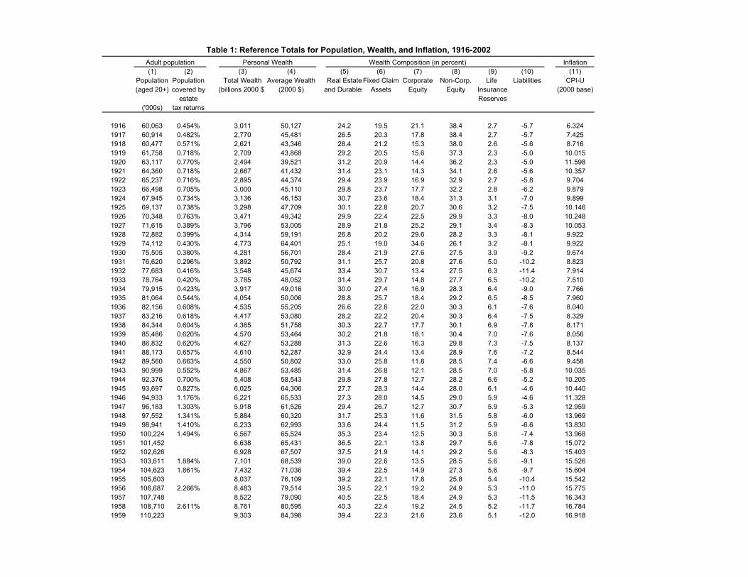
Wealth Composition (in percent) Inflation(1) (2) (3) (4) (5) (6) (7) (8) (9) (10) (11)

Population Population Total Wealth Average Wealth Real Estate Fixed Claim Corporate Non-Corp. Life Liabilities CPI-U(aged 20+) covered by (billions 2000 $) (2000 $) and Durables Assets Equity Equity Insurance (2000 base)

estate Reserves('000s) tax returns

1916 60,063 0.454% 3,011 50,127 24.2 19.5 21.1 38.4 2.7 -5.7 6.3241917 60,914 0.482% 2,770 45,481 26.5 20.3 17.8 38.4 2.7 -5.7 7.4251918 60,477 0.571% 2,621 43,346 28.4 21.2 15.3 38.0 2.6 -5.6 8.7161919 61,758 0.718% 2,709 43,868 29.2 20.5 15.6 37.3 2.3 -5.0 10.0151920 63,117 0.770% 2,494 39,521 31.2 20.9 14.4 36.2 2.3 -5.0 11.5981921 64,360 0.718% 2,667 41,432 31.4 23.1 14.3 34.1 2.6 -5.6 10.3571922 65,237 0.716% 2,895 44,374 29.4 23.9 16.9 32.9 2.7 -5.8 9.7041923 66,498 0.705% 3,000 45,110 29.8 23.7 17.7 32.2 2.8 -6.2 9.8791924 67,945 0.734% 3,136 46,153 30.7 23.6 18.4 31.3 3.1 -7.0 9.8991925 69,137 0.738% 3,298 47,709 30.1 22.8 20.7 30.6 3.2 -7.5 10.1461926 70,348 0.763% 3,471 49,342 29.9 22.4 22.5 29.9 3.3 -8.0 10.2481927 71,615 0.389% 3,796 53,005 28.9 21.8 25.2 29.1 3.4 -8.3 10.0531928 72,882 0.399% 4,314 59,191 26.8 20.2 29.6 28.2 3.3 -8.1 9.9221929 74,112 0.430% 4,773 64,401 25.1 19.0 34.6 26.1 3.2 -8.1 9.9221930 75,505 0.380% 4,281 56,701 28.4 21.9 27.6 27.5 3.9 -9.2 9.6741931 76,620 0.296% 3,892 50,792 31.1 25.7 20.8 27.6 5.0 -10.2 8.8231932 77,683 0.416% 3,548 45,674 33.4 30.7 13.4 27.5 6.3 -11.4 7.9141933 78,764 0.420% 3,785 48,052 31.4 29.7 14.8 27.7 6.5 -10.2 7.5101934 79,915 0.423% 3,917 49,016 30.0 27.4 16.9 28.3 6.4 -9.0 7.7661935 81,064 0.544% 4,054 50,006 28.8 25.7 18.4 29.2 6.5 -8.5 7.9601936 82,156 0.608% 4,535 55,205 26.6 22.6 22.0 30.3 6.1 -7.6 8.0401937 83,216 0.618% 4,417 53,080 28.2 22.2 20.4 30.3 6.4 -7.5 8.3291938 84,344 0.604% 4,365 51,758 30.3 22.7 17.7 30.1 6.9 -7.8 8.1711939 85,486 0.620% 4,570 53,464 30.2 21.8 18.1 30.4 7.0 -7.6 8.0561940 86,832 0.620% 4,627 53,288 31.3 22.6 16.3 29.8 7.3 -7.5 8.1371941 88,173 0.657% 4,610 52,287 32.9 24.4 13.4 28.9 7.6 -7.2 8.5441942 89,560 0.663% 4,550 50,802 33.0 25.8 11.8 28.5 7.4 -6.6 9.4581943 90,999 0.552% 4,867 53,485 31.4 26.8 12.1 28.5 7.0 -5.8 10.0351944 92,376 0.700% 5,408 58,543 29.8 27.8 12.7 28.2 6.6 -5.2 10.2051945 93,697 0.827% 6,025 64,306 27.7 28.3 14.4 28.0 6.1 -4.6 10.4401946 94,933 1.176% 6,221 65,533 27.3 28.0 14.5 29.0 5.9 -4.6 11.3281947 96,183 1.303% 5,918 61,526 29.4 26.7 12.7 30.7 5.9 -5.3 12.9591948 97,552 1.341% 5,884 60,320 31.7 25.3 11.6 31.5 5.8 -6.0 13.9691949 98,941 1.410% 6,233 62,993 33.6 24.4 11.5 31.2 5.9 -6.6 13.8301950 100,224 1.494% 6,567 65,524 35.3 23.4 12.5 30.3 5.8 -7.4 13.9681951 101,452 6,638 65,431 36.5 22.1 13.8 29.7 5.6 -7.8 15.0721952 102,626 6,928 67,507 37.5 21.9 14.1 29.2 5.6 -8.3 15.4031953 103,611 1.884% 7,101 68,539 39.0 22.6 13.5 28.5 5.6 -9.1 15.5261954 104,623 1.861% 7,432 71,036 39.4 22.5 14.9 27.3 5.6 -9.7 15.6041955 105,603 8,037 76,109 39.2 22.1 17.8 25.8 5.4 -10.4 15.5421956 106,687 2.266% 8,483 79,514 39.5 22.1 19.2 24.9 5.3 -11.0 15.7751957 107,748 8,522 79,090 40.5 22.5 18.4 24.9 5.3 -11.5 16.3431958 108,710 2.611% 8,761 80,595 40.3 22.4 19.2 24.5 5.2 -11.7 16.7841959 110,223 9,303 84,398 39.4 22.3 21.6 23.6 5.1 -12.0 16.918

Adult population Personal Wealth

Table 1: Reference Totals for Population, Wealth, and Inflation, 1916-2002

1960 111,314 2.950% 9,526 85,579 39.7 22.8 22.0 23.1 5.1 -12.7 17.1891961 112,450 9,978 88,733 39.1 22.8 23.4 22.6 5.0 -13.0 17.3611962 113,754 2.700% 10,382 91,268 38.7 23.0 24.2 22.4 5.0 -13.4 17.5521963 115,096 10,614 92,215 39.0 23.8 24.2 22.2 5.0 -14.3 17.7621964 116,796 11,108 95,103 38.5 24.2 25.7 21.5 4.9 -14.9 17.9931965 118,275 2.923% 11,737 99,231 37.5 24.2 27.5 21.1 4.8 -15.2 18.2991966 119,724 11,963 99,918 38.0 24.9 26.4 21.4 4.8 -15.6 18.8301967 121,143 12,425 102,562 38.1 25.3 26.2 21.2 4.7 -15.6 19.3761968 123,507 13,343 108,037 37.3 24.6 28.5 20.2 4.4 -15.0 20.1901969 125,543 4.069% 13,447 107,108 38.6 25.0 26.9 20.4 4.3 -15.1 21.2801970 127,674 13,026 102,028 40.3 26.2 23.7 20.9 4.4 -15.5 22.5351971 130,774 13,420 102,619 40.2 26.4 23.5 21.0 4.2 -15.3 23.5271972 133,502 5.343% 14,606 109,410 39.6 25.8 25.0 20.7 4.0 -15.1 24.2801973 136,006 14,885 109,446 41.4 26.1 22.4 21.9 3.8 -15.6 25.7851974 138,444 13,574 98,048 44.4 28.2 15.6 24.8 4.0 -17.0 28.6211975 141,055 13,232 93,809 45.1 29.1 13.4 25.7 4.0 -17.3 31.2261976 143,609 6.517% 14,136 98,433 44.5 28.3 15.2 25.1 3.7 -16.8 33.0371977 146,305 14,686 100,378 46.0 28.1 14.2 25.5 3.5 -17.3 35.1851978 149,142 15,125 101,413 48.2 28.0 12.1 26.4 3.4 -18.1 37.8591979 152,105 15,518 102,022 49.1 27.5 11.8 26.8 3.1 -18.3 42.1371980 155,268 15,701 101,122 48.8 26.8 12.8 26.7 2.9 -17.9 47.8251981 158,033 15,739 99,594 49.2 26.9 12.3 26.5 2.7 -17.6 52.7511982 160,665 1.966% 15,803 98,360 49.6 27.8 11.5 25.9 2.6 -17.5 56.0221983 163,135 1.800% 16,275 99,767 48.8 29.1 12.1 24.9 2.6 -17.5 57.8141984 165,650 1.483% 16,737 101,040 49.5 30.7 11.8 23.5 2.5 -18.0 60.3001985 168,205 1.178% 17,700 105,231 50.7 32.0 11.9 21.7 2.3 -18.7 62.4711986 170,556 1.147% 19,199 112,570 50.8 32.7 13.2 20.4 2.2 -19.3 63.6581987 172,552 1.125% 20,086 116,408 50.9 33.3 13.4 19.7 2.2 -19.5 65.9501988 174,344 1.046% 20,902 119,890 50.9 33.7 13.5 19.2 2.2 -19.4 68.6541989 176,060 1.192% 21,736 123,460 50.5 33.2 14.9 18.5 2.2 -19.3 71.9491990 178,365 1.305% 21,588 121,034 50.7 33.6 15.1 18.3 2.3 -20.0 75.8341991 180,978 1.312% 21,630 119,519 49.9 33.8 16.6 17.7 2.4 -20.4 79.0191992 183,443 1.371% 22,186 120,942 49.0 32.8 19.5 16.6 2.4 -20.3 81.3901993 185,685 1.504% 22,478 121,053 48.8 31.9 21.4 16.1 2.5 -20.6 83.8321994 187,757 1.541% 22,619 120,472 48.7 31.7 22.0 16.2 2.6 -21.3 86.0111995 189,911 1.598% 23,407 123,251 47.8 30.8 24.1 16.2 2.6 -21.5 88.4191996 192,043 1.808% 24,908 129,698 45.7 29.2 27.9 15.6 2.6 -21.0 91.0721997 194,426 1.930% 26,847 138,082 43.3 27.7 31.9 15.0 2.5 -20.4 93.1671998 196,795 2.032% 29,306 148,916 41.6 26.2 35.1 14.4 2.5 -19.8 94.6571999 199,255 2.206% 32,183 161,519 40.0 25.0 38.3 13.5 2.4 -19.2 96.7402000 201,865 2.072% 32,936 163,161 41.2 24.8 37.9 13.5 2.4 -19.8 100.0002001 204,323 31,510 154,217 45.6 26.5 33.0 14.2 2.6 -21.8 102.8462002 206,811 30,194 146,000 50.8 28.8 26.9 14.9 2.9 -24.2 104.472

Notes: Population estimates based on census data from Historical Statistics of the United States and the U.S. Statistical Abstract.Population covered by tax returns is defined by the population represented, using the multiplier technique, by estate tax returns with net worth above the filing threshold.Total wealth is defined as net worth of the personal sector excluding all future social security benefits and human wealth but including life insurance reserves.Only the cash surrender value of pension reserves is included (such as vested defined contribution and 401(k) accounts). The series is estimated from the Flow of Funds Accounts since 1945 and from several other sources before 1945. The series estimate average wealth during the corresponding year (and not end of year estimates). Wealth composition column reports the percent shares of tangible assets (owner occupied real estate and tenant occupied buildings with four units or less, consumer durables), fixed claim assets (cash and saving deposits, all bonds, mortgages), corporate equity, non-corporate equity (which includes tenant occupied net real estate for buildings with more than 4 units), and life insurance reserves. Liabilities include all debts (mortgages and consumer credit). Columns (5) to (10) add up to 100%. The Consumer Price Index (CPI) series is used to express all nominal values into real 2000 dollars.

Table 2

PercentilesWealth

Threshold Upper GroupsNumber of individuals

Average Wealth

(1) (2) (3) (4) (5)

Full Population 201,865,000 $163,161 2.00% $729,932 Top 2-1% 2,018,650 $920,0731.00% $1,172,896 Top 1-0.5% 1,009,325 $1,472,4560.50% $1,841,697 Top 0.5-0.25% 504,663 $2,314,0110.25% $3,067,676 Top 0.25-0.1% 302,798 $3,989,1320.10% $5,503,678 Top 0.1-0.05% 100,933 $6,717,8850.05% $8,219,720 Top 0.05-0.01% 80,746 $12,675,6290.01% $24,415,150 Top 0.01% 20,187 $63,564,151

Notes: Computations based on estate tax return statistics (see Appendix Section D in Kopczuk and Saez, 2004).

Wealth defined as total assets less liabilities. It includes the estimated cash surrender value of life insurance.

It excludes annuitized wealth, and future pensions with no cash surrender value, future labor income and

social security benefits. Amounts are expressed in 2000 dollars.

Source: Table 1 and Table B2, row 2000 in Kopczuk and Saez (2004)

Thresholds and Average Wealth in Top Groups within the Top 2% in 2000

2% 1% 0.50% 0.25% 0.10% 0.05% 0.01% 2-1% 1-.5% .5-.25% .25-.1% .1-.05% .05-.01%(1) (2) (3) (4) (5) (6) (7) (7) (8) (9) (10) (11)

1916 38.12 32.67 27.44 21.03 16.90 9.69 5.45 5.23 6.40 4.13 7.211917 35.58 30.17 25.15 19.31 15.47 8.85 5.41 5.02 5.84 3.84 6.621918 36.80 31.17 25.97 20.02 16.11 9.49 5.63 5.19 5.96 3.91 6.631923 39.93 33.82 28.42 22.39 18.38 11.32 6.11 5.40 6.03 4.01 7.061920 37.61 31.65 26.29 20.36 16.61 10.07 5.96 5.35 5.93 3.75 6.541921 35.22 29.12 23.68 17.54 13.68 7.48 6.10 5.43 6.15 3.86 6.201922 36.02 29.81 24.11 17.55 13.39 6.38 6.21 5.70 6.55 4.17 7.001923 35.22 29.49 24.13 17.80 13.66 6.84 5.73 5.35 6.34 4.14 6.821924 36.70 30.85 25.39 19.00 14.95 8.23 5.85 5.46 6.39 4.05 6.721925 36.02 30.08 24.77 18.45 14.55 7.79 5.94 5.32 6.31 3.90 6.761926 35.15 29.75 24.46 18.41 14.59 8.26 5.40 5.29 6.05 3.82 6.331927 39.21 33.19 27.72 21.28 17.19 10.16 6.02 5.46 6.45 4.09 7.031928 36.50 31.03 25.93 19.70 15.62 8.87 5.47 5.10 6.23 4.08 6.751929 36.76 31.84 26.91 20.80 16.65 9.15 4.92 4.93 6.11 4.16 7.491930 40.29 34.47 29.17 22.85 18.71 10.77 5.82 5.31 6.31 4.15 7.941931 34.70 29.47 24.63 18.77 14.87 8.25 5.23 4.84 5.85 3.90 6.621932 28.40 24.04 19.75 14.68 11.50 6.03 4.36 4.28 5.07 3.18 5.471933 30.31 25.80 21.46 16.28 12.91 6.91 4.51 4.34 5.18 3.37 6.001934 28.09 23.84 19.76 14.94 11.89 6.57 4.24 4.08 4.83 3.04 5.321935 27.77 23.76 19.69 14.98 11.88 6.54 4.01 4.08 4.71 3.10 5.341936 29.70 25.51 21.47 16.63 13.30 7.25 4.19 4.04 4.83 3.33 6.051937 26.97 22.64 18.73 14.22 11.37 6.14 4.32 3.91 4.52 2.85 5.231938 27.06 22.70 18.70 14.13 11.21 6.11 4.36 4.00 4.57 2.93 5.101939 25.95 21.59 17.65 13.18 10.40 5.56 4.36 3.94 4.47 2.78 4.841940 25.27 20.83 16.87 12.42 9.67 4.96 4.44 3.96 4.45 2.75 4.711941 25.30 20.74 16.71 12.35 9.67 5.02 4.56 4.03 4.37 2.67 4.651942 23.74 19.34 15.48 11.31 8.69 4.13 4.40 3.85 4.17 2.63 4.561943 24.26 19.46 15.35 10.96 8.35 4.23 4.80 4.11 4.39 2.62 4.111944 25.49 20.35 16.00 11.40 8.64 4.31 5.14 4.35 4.60 2.76 4.331945 24.65 19.38 15.05 10.54 7.92 3.69 5.27 4.33 4.51 2.62 4.231946 30.90 24.49 19.06 14.70 10.28 7.61 3.84 6.41 5.43 4.36 4.42 2.67 3.781947 31.07 24.28 18.81 14.57 10.26 7.76 4.07 6.79 5.46 4.25 4.30 2.50 3.691948 29.67 23.04 17.69 13.54 9.45 7.04 3.65 6.63 5.35 4.15 4.09 2.41 3.391949 29.42 22.59 17.25 13.08 9.03 6.69 3.33 6.83 5.34 4.17 4.04 2.35 3.361950 29.53 22.78 17.49 13.34 9.24 6.96 3.49 6.75 5.28 4.15 4.10 2.27 3.481953 30.91 23.77 18.26 13.95 9.73 7.31 3.60 7.14 5.52 4.31 4.22 2.42 3.721954 29.99 23.18 17.89 13.71 9.60 7.31 3.74 6.81 5.30 4.18 4.11 2.29 3.561956 31.49 24.75 19.25 14.89 10.48 7.93 3.99 6.74 5.50 4.35 4.41 2.55 3.941958 31.19 24.18 18.64 14.35 10.06 7.69 4.15 7.01 5.55 4.29 4.28 2.38 3.541960 32.45 25.25 19.50 15.02 10.53 7.99 4.14 7.21 5.75 4.48 4.49 2.54 3.851962 31.01 24.39 19.06 14.74 10.36 7.88 4.03 6.61 5.33 4.32 4.38 2.47 3.861965 30.75 24.70 19.59 15.35 10.85 8.27 4.41 6.05 5.10 4.25 4.50 2.58 3.861969 29.11 22.86 17.84 13.84 9.87 7.64 4.34 6.25 5.02 4.00 3.98 2.22 3.301972 29.52 23.13 18.06 14.03 9.89 7.47 3.99 6.39 5.07 4.02 4.14 2.42 3.481976 25.67 19.32 14.52 10.91 7.45 5.63 2.91 6.35 4.80 3.61 3.46 1.83 2.721982 25.17 19.06 14.36 10.79 7.33 5.40 2.53 6.11 4.70 3.56 3.47 1.93 2.871983 26.96 21.07 15.93 12.06 8.40 6.40 3.19 5.89 5.15 3.87 3.66 1.99 3.211984 26.57 20.95 16.23 12.23 8.60 6.62 3.51 5.62 4.72 4.00 3.63 1.99 3.101985 28.49 22.35 17.43 13.49 9.45 7.25 4.09 6.14 4.92 3.95 4.04 2.20 3.161986 28.80 22.66 17.62 13.63 9.61 7.37 3.91 6.14 5.03 4.00 4.02 2.23 3.461987 27.78 21.57 16.66 12.79 8.98 6.73 3.44 6.22 4.91 3.88 3.80 2.25 3.291988 27.77 21.70 16.85 12.92 8.95 6.80 3.60 6.07 4.86 3.93 3.97 2.15 3.211989 28.04 21.96 17.02 13.13 9.30 7.11 3.79 6.08 4.94 3.89 3.83 2.19 3.321990 27.39 20.86 15.95 12.21 8.73 6.78 3.63 6.53 4.91 3.74 3.48 1.95 3.151991 27.73 21.54 16.56 12.73 8.95 6.79 3.55 6.20 4.98 3.83 3.78 2.16 3.241992 27.23 21.18 16.34 12.66 8.99 6.88 3.72 6.06 4.84 3.68 3.67 2.12 3.161993 27.53 21.31 16.33 12.44 8.69 6.72 3.76 6.22 4.98 3.89 3.75 1.98 2.961994 28.08 21.58 16.63 12.84 9.00 6.96 3.86 6.50 4.96 3.79 3.84 2.04 3.111995 27.74 21.54 16.67 12.91 9.29 7.23 3.99 6.20 4.87 3.76 3.62 2.07 3.241996 27.68 21.45 16.51 12.71 9.08 6.98 3.84 6.23 4.94 3.80 3.63 2.10 3.151997 27.24 21.24 16.41 12.56 8.92 6.91 3.78 6.00 4.83 3.85 3.64 2.01 3.131998 27.67 21.70 16.86 13.08 9.38 7.31 3.99 5.97 4.83 3.78 3.70 2.08 3.321999 27.68 21.68 16.86 13.16 9.40 7.28 3.91 6.00 4.82 3.69 3.76 2.12 3.372000 26.43 20.79 16.27 12.73 9.06 7.00 3.90 5.64 4.51 3.55 3.67 2.06 3.11

Notes: Computations by authors based on estate tax return statistics. See Appendix Section D in Kopczuk and Saez (2004) for details.Series display the top of total net-worth accruing to each upper wealth group.Series for Top 2-1% are estimated only for the 1946-2000 period because the tax return population does not cover that group in the pre-war period.

Table 3: Top Wealth Shares in the United States, 1916-2000

Top groups Intermediate Groups

Real Bonds StockLife Ins Other Debts Real Bonds StockLife Ins Other Debts Real Bonds StockLife Ins Other Debts Real Bonds StockLife Ins Other Debts Real Bonds StockLife Ins Other Debts1916 1916 1916 28.1 35.5 36.4 0.3 7.8 -8.1 1916 23.6 36.5 39.1 0.3 7.2 -6.7 1916 19.7 37.5 41.4 0.3 7.4 -6.31917 1917 1917 29.5 32.3 39.9 0.4 6.2 -8.2 1917 24.8 32.4 44.0 0.3 5.9 -7.4 1917 19.9 31.1 49.4 0.3 5.8 -6.51918 1918 1918 27.7 33.3 40.1 0.5 8.3 -10.0 1918 23.9 33.5 43.5 0.4 8.1 -9.4 1918 19.7 33.4 47.4 0.3 7.7 -8.41919 1919 1919 25.1 29.9 45.3 1.0 9.2 -10.4 1919 21.0 30.0 48.9 0.8 8.9 -9.7 1919 17.1 30.3 52.1 0.7 9.2 -9.41920 1920 1920 24.2 28.1 49.4 1.3 8.8 -11.7 1920 20.1 27.5 53.7 1.1 8.4 -10.8 1920 16.3 26.3 58.8 0.8 7.7 -10.01921 1921 1921 29.9 32.1 42.1 2.0 7.7 -13.7 1921 26.9 32.0 45.7 1.7 8.0 -14.3 1921 23.9 32.0 50.2 1.2 8.3 -15.61922 1922 1922 27.3 32.5 44.0 2.4 7.2 -13.6 1922 24.3 31.8 48.6 2.1 7.3 -14.1 1922 21.4 30.5 54.6 1.4 7.4 -15.31923 1923 1923 25.7 30.6 46.5 2.5 6.9 -12.2 1923 22.4 29.5 51.6 2.2 6.7 -12.5 1923 18.6 28.2 58.4 1.6 6.3 -13.11924 1924 1924 22.5 33.2 45.1 2.4 7.3 -10.6 1924 19.4 32.8 49.1 1.8 7.3 -10.3 1924 15.7 32.4 53.4 1.0 7.3 -9.81925 1925 1925 21.9 31.3 46.7 2.3 8.2 -10.3 1925 19.0 30.3 50.7 1.9 8.3 -10.2 1925 16.1 29.2 56.0 1.2 8.0 -10.41926 1926 1926 1926 19261927 1927 1927 18.7 28.5 54.7 2.4 6.4 -10.7 1927 16.1 27.2 58.9 2.0 6.3 -10.6 1927 13.2 25.4 64.9 1.2 6.2 -10.91928 1928 1928 17.4 24.1 58.1 2.2 7.9 -9.7 1928 13.9 23.5 62.3 1.7 7.8 -9.2 1928 10.8 21.5 66.4 1.3 7.7 -7.81929 1929 1929 15.6 26.6 58.9 1.6 8.1 -10.7 1929 12.7 26.2 62.1 1.3 7.9 -10.2 1929 10.2 25.1 65.1 1.0 8.1 -9.41930 1930 1930 15.3 29.1 58.1 2.4 7.4 -12.4 1930 13.3 28.1 61.7 1.7 7.7 -12.5 1930 10.7 27.2 65.1 1.5 7.8 -12.31931 1931 1931 17.5 34.4 48.3 4.0 8.0 -12.1 1931 16.0 33.6 50.8 3.4 8.5 -12.3 1931 13.6 32.6 54.8 2.1 9.3 -12.51932 1932 1932 19.1 38.6 42.5 5.1 16.8 -22.0 1932 17.7 36.9 46.0 4.2 19.4 -24.2 1932 15.2 34.9 51.0 2.5 24.3 -28.01933 1933 1933 19.4 40.4 41.9 4.9 9.2 -15.8 1933 17.8 40.2 44.6 3.9 9.8 -16.4 1933 16.1 39.8 48.6 2.5 11.1 -18.21934 1934 1934 17.7 38.5 46.8 4.5 9.4 -17.0 1934 16.2 37.7 50.7 3.7 10.1 -18.3 1934 14.1 36.2 56.9 2.5 11.3 -21.11935 1935 1935 15.8 38.7 43.8 4.3 9.4 -12.0 1935 13.8 37.8 47.1 3.5 10.0 -12.2 1935 10.9 36.5 52.1 2.2 11.2 -13.01936 1936 1936 14.1 36.3 50.3 2.0 6.8 -9.6 1936 11.2 35.5 53.9 1.9 6.9 -9.3 1936 8.1 34.6 58.4 1.4 6.9 -9.41937 1937 1937 15.8 36.3 48.9 2.1 7.4 -10.5 1937 13.2 35.6 52.4 1.9 7.5 -10.6 1937 10.9 35.0 56.3 1.5 7.7 -11.31938 1938 1938 15.2 35.5 45.7 3.0 9.0 -8.4 1938 12.5 35.0 48.8 2.4 9.1 -7.8 1938 9.0 34.8 50.6 1.9 9.4 -5.71939 1939 1939 14.9 34.1 49.3 3.2 7.1 -8.7 1939 12.3 33.9 52.6 2.8 6.4 -8.0 1939 9.2 34.0 56.3 2.1 5.7 -7.21940 1940 1940 16.6 34.4 45.0 3.2 9.3 -8.5 1940 13.9 34.5 48.0 2.6 9.0 -7.9 1940 11.4 34.5 51.7 1.9 8.1 -7.71941 1941 1941 20.9 40.6 45.3 1.3 6.2 -14.3 1941 17.8 40.7 48.9 1.3 6.1 -14.8 1941 14.1 41.5 52.4 1.2 5.6 -14.71942 1942 1942 20.3 35.7 49.4 1.2 6.5 -13.1 1942 17.1 35.1 53.9 1.2 6.4 -13.7 1942 13.6 34.1 59.4 1.1 6.1 -14.11943 1943 1943 19.4 35.1 50.2 1.4 7.9 -14.0 1943 16.4 34.6 55.3 1.4 7.6 -15.3 1943 13.0 34.1 61.7 1.4 7.1 -17.31944 1944 1944 15.2 31.9 46.3 3.2 9.7 -6.3 1944 12.5 31.8 49.8 2.7 8.9 -5.8 1944 10.5 31.5 53.6 2.2 7.2 -4.91945 1945 1945 1945 19451946 25.4 34.1 39.1 0.9 7.4 -6.0 1946 22.5 32.9 42.7 0.9 7.4 -6.4 1946 18.9 32.7 46.9 0.8 7.1 -6.5 1946 16.0 32.7 50.4 0.7 6.5 -6.3 1946 13.2 32.8 53.6 0.5 5.8 -5.91947 26.2 34.3 37.8 1.0 8.1 -6.4 1947 23.0 32.9 41.9 0.9 8.1 -6.8 1947 19.4 32.9 46.1 0.8 7.7 -6.8 1947 16.1 33.2 49.5 0.7 7.0 -6.5 1947 13.0 33.5 52.7 0.5 6.3 -5.91948 27.0 34.4 37.2 1.0 8.0 -6.5 1948 23.5 32.6 41.7 1.0 8.1 -6.9 1948 19.9 32.4 46.0 0.9 7.9 -7.0 1948 16.5 32.5 49.7 0.7 7.3 -6.8 1948 13.3 32.6 53.3 0.5 6.6 -6.31949 27.4 33.2 37.7 1.0 8.2 -6.5 1949 24.0 31.6 42.2 1.0 8.4 -7.1 1949 20.5 31.1 46.7 0.9 8.2 -7.2 1949 17.5 30.9 50.4 0.7 7.8 -7.4 1949 14.6 30.8 54.1 0.6 7.3 -7.41950 27.1 33.1 38.4 0.9 8.3 -6.8 1950 23.7 31.5 42.9 0.9 8.4 -7.4 1950 20.3 31.0 47.4 0.8 8.2 -7.7 1950 17.6 30.8 50.9 0.7 7.9 -7.9 1950 15.0 30.7 54.6 0.5 7.4 -8.21953 25.4 28.7 42.9 0.9 9.0 -6.1 1953 21.4 27.0 48.2 0.8 8.9 -6.3 1953 17.8 26.4 52.9 0.7 8.5 -6.3 1953 14.4 26.2 57.0 0.6 7.9 -6.1 1953 10.9 26.0 61.1 0.4 7.2 -5.61954 25.1 27.7 43.8 0.8 9.1 -5.7 1954 21.1 25.8 49.2 0.8 9.2 -6.0 1954 17.4 25.2 53.9 0.7 8.9 -6.0 1954 14.4 24.5 57.7 0.6 8.5 -5.7 1954 11.2 23.8 61.8 0.4 8.2 -5.41956 23.6 26.3 47.0 0.8 8.9 -5.8 1956 19.6 24.7 52.1 0.7 8.8 -5.9 1956 16.2 24.0 56.6 0.6 8.5 -5.9 1956 13.3 23.5 60.3 0.5 8.2 -5.6 1956 10.6 23.1 63.6 0.3 7.7 -5.51958 23.8 25.2 48.0 0.7 8.9 -5.9 1958 19.9 23.5 53.1 0.6 8.8 -6.0 1958 16.6 22.7 57.5 0.5 8.6 -6.0 1958 13.8 22.3 61.2 0.4 8.2 -5.9 1958 11.2 22.1 64.4 0.3 7.8 -5.91960 21.5 24.6 51.6 0.7 7.8 -5.5 1960 17.9 22.8 56.5 0.6 7.7 -5.5 1960 14.7 22.0 60.6 0.5 7.5 -5.3 1960 12.1 21.4 63.9 0.4 7.3 -5.1 1960 9.3 21.0 67.0 0.3 7.2 -4.81962 20.1 23.7 52.9 1.0 10.1 -6.8 1962 17.1 21.1 57.7 1.0 10.1 -6.9 1962 14.6 19.8 62.0 1.0 9.7 -7.1 1962 12.8 19.0 65.7 1.1 9.0 -7.5 1962 9.7 18.8 70.1 0.6 8.3 -7.51965 20.3 26.3 53.5 1.3 4.7 -4.9 1965 17.1 23.4 58.9 1.1 4.4 -4.9 1965 14.5 22.1 63.4 0.9 4.1 -4.9 1965 12.4 21.3 66.8 0.7 3.8 -5.0 1965 10.3 20.8 70.0 0.5 3.5 -5.11969 23.6 25.9 48.7 2.3 12.4 -10.5 1969 19.9 22.3 53.5 1.8 12.7 -10.2 1969 17.1 21.2 58.0 1.4 12.5 -10.2 1969 14.4 20.3 61.5 1.1 13.1 -10.4 1969 10.8 18.8 65.6 0.8 13.8 -9.91972 24.7 27.8 46.3 2.0 10.6 -9.4 1972 21.3 24.3 51.3 1.6 10.6 -9.1 1972 18.8 21.9 56.5 1.3 10.3 -8.7 1972 16.2 20.5 60.3 1.0 10.4 -8.3 1972 13.6 19.1 64.2 0.7 10.3 -7.81976 31.7 30.8 35.8 2.3 12.2 -10.5 1976 28.3 27.4 40.4 1.7 12.5 -10.3 1976 24.4 27.4 44.5 1.4 12.3 -10.1 1976 20.0 27.4 48.2 1.1 12.7 -9.5 1976 16.1 26.7 52.9 0.8 13.1 -9.61982 1982 34.4 23.6 32.1 2.1 18.8 -11.0 1982 31.2 22.4 35.3 1.8 19.3 -10.1 1982 28.4 21.2 38.4 1.5 20.2 -9.7 1982 25.0 19.9 41.7 1.2 21.2 -9.11983 1983 32.0 23.6 33.0 2.5 18.6 -9.7 1983 28.6 23.1 36.1 2.1 19.1 -9.1 1983 25.1 22.9 41.3 1.3 18.4 -9.0 1983 23.4 19.9 45.4 1.0 20.7 -10.41984 1984 33.1 25.1 33.5 2.1 18.3 -12.1 1984 31.7 23.8 37.6 1.7 17.8 -12.6 1984 27.7 23.5 40.8 1.1 18.6 -11.8 1984 24.0 21.5 45.1 1.0 20.1 -11.81985 1985 27.2 24.9 37.2 2.2 17.8 -9.3 1985 25.6 23.5 40.6 1.7 17.7 -9.1 1985 23.3 22.4 44.2 1.4 17.3 -8.7 1985 18.3 21.1 50.5 0.9 16.8 -7.51986 1986 27.1 24.1 37.5 1.9 19.0 -9.6 1986 24.4 22.8 41.5 1.6 19.0 -9.2 1986 22.6 20.6 45.6 1.3 19.3 -9.4 1986 19.2 18.7 52.1 1.1 18.3 -9.41987 1987 27.8 24.9 33.5 2.3 20.5 -8.9 1987 25.3 23.4 36.5 2.0 21.4 -8.6 1987 23.0 21.8 40.3 1.5 22.2 -8.9 1987 21.0 20.8 42.7 1.2 23.5 -9.21988 1988 30.3 26.4 31.9 2.7 17.4 -8.7 1988 28.0 24.9 35.4 2.6 17.6 -8.5 1988 25.2 24.6 38.7 2.3 17.3 -8.1 1988 23.1 22.7 42.6 2.2 17.2 -7.91989 1989 30.2 25.1 29.0 2.1 22.1 -8.5 1989 28.1 23.7 31.8 1.8 22.9 -8.3 1989 26.2 22.2 34.1 1.4 24.0 -7.9 1989 22.2 21.2 36.6 1.0 25.7 -6.61990 1990 28.5 28.9 27.8 2.0 21.0 -8.3 1990 26.2 28.2 30.2 1.6 21.9 -8.1 1990 24.5 27.8 32.7 1.2 21.8 -8.1 1990 20.7 27.1 35.4 1.0 23.7 -7.91991 1991 25.8 28.5 31.8 2.1 20.1 -8.3 1991 24.0 27.4 35.2 1.7 19.8 -8.1 1991 21.7 26.5 38.6 1.4 19.9 -8.1 1991 18.4 24.5 43.4 1.1 20.3 -7.81992 1992 23.3 25.5 39.7 1.9 16.7 -7.1 1992 21.4 24.3 44.2 1.5 15.7 -7.0 1992 19.1 23.3 47.9 1.2 15.1 -6.6 1992 15.9 22.0 52.8 0.9 13.6 -5.31993 1993 20.3 26.9 39.7 2.0 17.2 -6.2 1993 17.9 26.3 44.0 1.6 15.9 -5.8 1993 16.0 25.9 47.5 1.4 14.6 -5.4 1993 14.2 22.4 53.9 1.0 13.5 -5.11994 1994 23.8 29.1 33.5 2.1 18.5 -7.0 1994 21.3 29.2 37.1 1.7 17.7 -6.9 1994 19.2 28.7 40.4 1.4 16.9 -6.5 1994 16.9 27.9 45.7 1.2 14.9 -6.61995 1995 25.7 25.4 34.6 2.0 19.0 -6.7 1995 23.9 24.6 38.5 1.5 17.9 -6.5 1995 22.7 23.0 42.4 1.1 16.9 -6.2 1995 21.3 21.3 46.5 0.8 15.8 -5.71996 24.1 27.5 34.6 2.6 20.9 -7.2 1996 21.9 24.5 38.6 2.0 19.6 -6.6 1996 20.0 24.0 42.8 1.6 18.2 -6.6 1996 18.4 22.9 46.5 1.3 17.3 -6.5 1996 17.0 21.2 51.7 0.9 15.8 -6.71997 23.2 26.5 36.8 2.1 20.4 -6.8 1997 20.9 23.8 40.5 1.8 19.4 -6.4 1997 19.0 23.2 44.6 1.4 18.0 -6.1 1997 17.7 22.5 47.9 1.1 16.6 -5.8 1997 16.2 20.7 52.7 0.9 15.6 -6.01998 22.5 27.3 40.6 2.3 16.1 -6.4 1998 20.3 24.6 44.5 1.9 14.9 -6.2 1998 18.5 23.7 48.3 1.5 14.0 -6.0 1998 16.9 22.8 51.3 1.1 13.9 -5.9 1998 15.1 21.3 56.1 0.7 12.8 -5.91999 22.1 25.3 37.7 2.0 21.0 -6.2 1999 20.0 22.9 41.5 1.4 20.1 -6.0 1999 18.3 22.8 44.4 1.1 19.0 -5.6 1999 17.2 22.8 47.5 0.9 17.2 -5.5 1999 15.1 22.5 51.6 0.6 15.8 -5.62000 23.9 23.3 36.9 2.1 22.7 -6.8 2000 22.5 20.8 39.9 1.6 22.0 -6.8 2000 21.0 19.6 43.9 1.2 20.8 -6.6 2000 19.5 20.0 46.2 0.9 20.0 -6.7 2000 17.4 19.8 47.8 0.8 21.0 -6.8Notes: Wealth is defined as all sources of (non-human) wealth net of debts and liabilities but excludes annuities, and claims on future pensions. Real is defined as real estate. Bonds is the sum of federal, local, foreign, and corporate bonds. Stock is corporate stockCash is currency, deposits, and notes. Other is equity in unincorporated business, and miscellaneous assetsThe sums of all sources less debts add up to 100%.

Top 0.1%Table 4: Composition by Sources of Wealth and by Fractiles of Total Wealth in the United States, 1916-2000

Top 2% Top 1% Top 0.5% Top 0.25%

Author Kopczuk-Saez Lampman (1962) Smith (1984) Wolff-Marley (1989) Wolff (1995) Scholz (2003)Unit Adults Adults Individuals Individuals Households HouseholdsData Estates Estates Estates Patched Estates Patched SCF-Estates SCF

Wealth Net Worth Net Worth Net Worth Total Assets Net Worth Net Worth(1) (2) (3) (4) (5) (6)

1922 36.02 31.6 34.0 36.71929 36.76 36.3 37.2 44.21933 30.31 28.3 31.3 33.31939 25.95 30.6 38.1 36.41945 24.65 23.3 28.9 29.81949 22.59 20.8 25.7 27.11953 23.77 24.3 28.1 31.21954 23.18 24.01956 24.75 26.01958 24.18 26.6 27.01962 24.39 28.2 30.1 31.8 31.61965 24.70 25.4 31.9 34.41969 22.86 27.4 29.0 31.11972 23.13 21.9 28.6 29.11976 19.32 19.2 18.9 19.91983 21.07 30.9 31.51986 22.66 31.91989 21.96 35.7 30.01992 21.18 30.01995 21.54 35.31998 21.70 34.12000 20.79

Notes: Lampman (1962), Table 94, p. 204, estimates are based on all estate tax returns filers and Pareto interpolation to optain top 1% share. Smith (1984), Table 1, p. 422, ranks individuals by total assets (not net worth) and defines top 1% group relative to total population (not only adults), and reports share of net-worth for this group.Wolff-Marley (1989), Table 6, p. 786, row W2, completed and corrected in Wolff (1995), Table A1, pp. 78-79, col. (1), "Wolff-Marley series".Top 1% defined relative to total population (not only adults). Estimates based on previous estimates by Lampman (1962) and Smith (1984).Wolff (1995), Table A1, pp. 78-79, col. (6) "New Household Series" based on previous "Wolff-Marley" series and SCF estimations. Scholz (2003) based on SCF data.

Table 5: Comparing Top 1% Wealth Share with Previous Estimates

Very Top Wealth Shares Ratio to Average Wealth Top Estate Share(1) (2) (3) (4) (5) (6) (7) (8) (9)

Forbes 400 Forbes 400 Top .0002% Top .00005% Top .0002-.00005% Top .0002% Top .00005% Top .0002-.00005% Top .01%Total Wealth Average Wealth (top 404 (top 101 (rank 102 to 404 (top 404 (top 101 (rank 102 to 404 Share

(billions 2000 $)(millions 2000 $) in 2000) in 2000) in 2000) in 2000) in 2000) in 2000) (top 20,000 in 2000)

1982 164.2 411 0.984 0.521 0.510 4,922 10,414 3,400 2.5251983 204.1 510 1.187 0.593 0.593 5,933 11,864 3,957 3.1941984 207.3 518 1.165 0.595 0.570 5,826 11,909 3,799 3.5141985 214.5 536 1.153 0.567 0.586 5,763 11,335 3,905 4.0851986 245.1 613 1.217 0.628 0.589 6,084 12,560 3,926 3.9131987 333.6 834 1.603 0.856 0.747 8,017 17,129 4,979 3.4381988 320.4 801 1.486 0.797 0.689 7,430 15,946 4,592 3.5961989 373.1 933 1.670 0.885 0.785 8,349 17,702 5,232 3.7911990 359.5 899 1.635 0.868 0.767 8,173 17,360 5,110 3.6311991 363.4 909 1.658 0.932 0.726 8,291 18,649 4,839 3.5491992 369.3 923 1.655 0.946 0.709 8,277 18,930 4,726 3.7151993 390.6 977 1.735 1.000 0.735 8,676 20,001 4,901 3.7611994 405.2 1,013 1.799 1.049 0.750 8,994 20,976 5,001 3.8571995 446.0 1,115 1.923 1.142 0.781 9,614 22,841 5,205 3.9881996 514.0 1,285 2.089 1.221 0.868 10,444 24,424 5,785 3.8361997 669.5 1,674 2.537 1.552 0.985 12,687 31,042 6,569 3.7781998 779.3 1,948 2.715 1.751 0.965 13,577 35,017 6,431 3.9871999 1033.0 2,582 3.286 2.268 1.018 16,429 45,355 6,787 3.9102000 1200.1 3,000 3.743 2.510 1.233 18,715 50,202 8,219 3.8962001 925.1 2,313 3.031 1.971 1.060 15,157 39,428 7,0662002 860.0 2,150 2.958 1.909 1.049 14,791 38,184 6,993

Notes: Data source is the Forbes 400 Richest American list published annually in October by Forbes Magazine since 1982.Columns (1) and (2) report the total wealth and average wealth of the Forbes 400 richest (in 2000 dollars, CPI from Table 1)Columns (3) to (5) report the share of total wealth (reported in Table 1, col. (3)) for the top .0002%, the top .00005%, and the top .0002-.00005% estimated using the Forbes list.The top .0002% corresponds to the top 404 richest americans in 2000. The top .00005% corresponds to the top 101 richest Americans in 2000.The top .0002-.00005% corresponds to the Americans with wealth rank 102 to 404 in 2000.Columns (6) to (8) report the ratio of the average wealth in the top .0002%, the top .00005%, and the top .0002-.00005% to the average wealth in the United States (from col. (4) in Table 1).Column (9) report the top .01% wealth share estimated from tax returns (from Table 3, col. (7)).

Table 6: Very Top Shares from Forbes 400 Richest Americans

FIGURE 1Average Real Wealth and Consumer Price Index in the United States, 1916-2002

Source: Table 1, columns Average Wealth (in real 2000 dollars) and CPI (base 100 in 2000)

$0

$20,000

$40,000

$60,000

$80,000

$100,000

$120,000

$140,000

$160,000

$180,000

1916

1921

1926

1931

1936

1941

1946

1951

1956

1961

1966

1971

1976

1981

1986

1991

1996

2001

Wea

lth in

200

0 D

olla

rs

1

10

100

Con

sum

er P

rice

Inde

x (b

ase

100

in 2

000)

Average Wealth Corporate EquityWealth less corp. equity Consumer Price Index

FIGURE 2The Top 1% Wealth Share in the United States, 1916-2000

Source: Table 3, col. Top 1%.

0%

5%

10%

15%

20%

25%

30%

35%

40%

45%

1916

1921

1926

1931

1936

1941

1946

1951

1956

1961

1966

1971

1976

1981

1986

1991

1996

Wea

lth S

hare

FIGURE 3Average Real Wealth of bottom 99% and top 1% in the United States, 1916-2000

Source: Table B2 in Kopczuk and Saez (2004), columns Top 1%, Bottom 99% computed from Average Wealth (Table 1, Col. (4)) and Average Top 1% wealth. Amounts are expressed in 2000 dollars

$0

$500,000

$1,000,000

$1,500,000

$2,000,000

$2,500,000

$3,000,000

$3,500,000

$4,000,000

1916

1921

1926

1931

1936

1941

1946

1951

1956

1961

1966

1971

1976

1981

1986

1991

1996

Ave

rage

Wea

lth o

f bot

tom

99%

$0

$20,000

$40,000

$60,000

$80,000

$100,000

$120,000

$140,000

$160,000

Ave

rage

Wea

lth o

f Top

1%

Top 1% average wealth

Bottom 99% average wealth

FIGURE 4The Wealth Shares of Top 2-1%, 1-0.5%, and 0.5-0.1%, 1916-2000

Source: Table 3, columns Top 2-1%, 1-0.5%, and 0.5-0.1%. Estimates for Top 2-1% are only available from 1946.

0%

2%

4%

6%

8%

10%

12%

14%19

16

1921

1926

1931

1936

1941

1946

1951

1956

1961

1966

1971

1976

1981

1986

1991

1996

Wea

lth S

hare

Top 2-1% Top 1-0.5% Top 0.5-0.1%

FIGURE 5The Shares of the Top Wealth Groups in the United States, 1916-2000

Source: Table 3, Columns 0.1%, and 0.01%.

A. Wealth share of the top 0.1%

0%

5%

10%

15%

20%

25%19

16

1921

1926

1931

1936

1941

1946

1951

1956

1961

1966

1971

1976

1981

1986

1991

1996

B. Wealth share of the top 0.01%

0.0%

2.0%

4.0%

6.0%

8.0%

10.0%

12.0%

1916

1921

1926

1931

1936

1941

1946

1951

1956

1961

1966

1971

1976

1981

1986

1991

1996

FIGURE 6Wealth Composition of Top Groups within the Top 0.5% in 1929

Source: Table 4, row 1929.Sum of four categories is 100%. Category debt has been excluded.

0%

10%

20%

30%

40%

50%

60%

70%

80%

.5-.2

5%

.25-

.1%

.1-.0

5%

.05-

.01%

Top

.01%

Real Estate Bonds and Cash Stock Other

FIGURE 7Fraction of Corporate Stock within the Top .5% and total net-worth, 1916-2000

Source: Table 1, Column (7) and Table 4, Top .5%, column stock.

0%

10%

20%

30%

40%

50%

60%

70%

1916

1921

1926

1931

1936

1941

1946

1951

1956

1961

1966

1971

1976

1981

1986

1991

1996

Frac

tion

(in %

)Fraction Stock in top .5% Fraction Stock in total net-worth

FIGURE 8Average Age and Fraction Female in Top 0.5%, 1916-2000

Source: Table B4 in Kopczuk and Saez (2004), columns age and fraction female.

0

10

20

30

40

50

60

7019

16

1921

1926

1931

1936

1941

1946

1951

1956

1961

1966

1971

1976

1981

1986

1991

1996

Age

and

per

cent

age

fem

ale

Average Age Percent Female

FIGURE 9The Top 0.01% Income Share and Composition, 1916-2000

The Figure displays the top 0.01% income share (top curve). Estimates are based on families and not individuals.Taxpayers are ranked by income excluding capital gains but capital gains included in the share.Interest, Rents, Trusts, etc.),The Figure displays the composition of those top incomes into Capital Income (Dividends, Realized Capital Gains, Business Income (Sole Proprietorships, Partnerships, S-Corporations), and Salaries (Wages and Salaries, Pensions).Source: Piketty and Saez (2003), series updated to year 2000

0.0%

0.5%

1.0%

1.5%

2.0%

2.5%

3.0%

3.5%

4.0%

4.5%19

16

1921

1926

1931

1936

1941

1946

1951

1956

1961

1966

1971

1976

1981

1986

1991

1996

Capital Income Capital Gains Business Income Salaries

FIGURE 10Marginal Tax Rate and Wealth Share for the Top 0.1%, 1916-2000

Notes: Marginal Tax Rate computations are made assuming no deductions beyond the basic exemption.Effective marginal tax rates are lower due to additional deductions (funeral expenses, spousal bequest deductions, charitable bequests, etc.)

0%

10%

20%

30%

40%

50%

60%

70%

80%

90%

100%19

16

1921

1926

1931

1936

1941

1946

1951

1956

1961

1966

1971

1976

1981

1986

1991

1996

Mar

gina

l Tax

Rat

e

0%

5%

10%

15%

20%

25%

Top

0.1%

Wea

lth S

hare

Top 0.1% Marginal Tax Rate Top marginal tax rate

Top 0.1% Share

FIGURE 11The Top 1% Wealth Share: Comparing Various Estimates

Source: Table 5

0%

5%

10%

15%

20%

25%

30%

35%

40%

45%

1916

1921

1926

1931

1936

1941

1946

1951

1956

1961

1966

1971

1976

1981

1986

1991

1996

Wea

lth S

hare

(in

%)

Kopczuk-Saez (Estates)

Lampman (Estates)

Smith (Estates)

Scholz (SCF)

Wolff (Estates-SCF)

FIGURE 12Very Top Shares from Forbes 400 Richest Americans, 1983-2002

Source: Table 6, col. (3), (4), (5), and (9). Year 1982 has been excluded because, as the first survey year, the Forbes list missed a number of fortunes.

0.0%

0.5%

1.0%

1.5%

2.0%

2.5%

3.0%

3.5%

4.0%

1983

1984

1985

1986

1987

1988

1989

1990

1991

1992

1993

1994

1995

1996

1997

1998

1999

2000

2001

2002

Wea

lth S

hare

(in

%)

Top .0002% (top 400 in 2000)

Top .00005% (top 100 in 2000)

Top .0002-.00005% (101 to 400 in 2000)