Too Much Skin-in-the-Game?

The Effect of Mortgage Market Concentration on Credit

and House Prices

Deeksha Gupta∗

January 28, 2019

Abstract

During the housing boom, a small number of institutions - the government-sponsored

enterprises (GSEs) and a few banks - held large shares of U.S. mortgage risk. I

develop a theory where such concentration of mortgage risk can explain key features

of the housing crisis. In the model, lenders with many outstanding mortgages have

incentives to extend risky credit to prop up house prices. At the onset of downturns,

large lenders will continue risky lending for a short period of time. This can explain

evidence documenting high-risk lending by the GSEs during the bust. The expectation

of continued risky lending during busts, worsens lending standards during preceding

booms through a feedback effect. More concentrated mortgage market exposure leads

to larger and riskier credit booms and busts.

Keywords: Concentration, GSEs, housing booms and busts, mortgage credit.

JEL Classifications: G01, G21, L11, L25, R21, R31.

∗The Tepper School, Carnegie Mellon University. I am deeply indebted to my dissertation committee:Itay Goldstein, Vincent Glode, Benjamin Keys, David Musto, and Christian Opp for their insightfulcomments, guidance, and support. I am also thankful to Anna Cororaton, Aycan Corum, Tetiana Davydiuk,Mehran Ebrahimian, Ronel Elul, Joao Gomes, Daniel Greenwald, Marco Grotteria, Ben Hyman, JessicaJeffers, Mete Kilic, Tim Landvoigt, Doron Levit, Pricila Maziero, Thien Nguyen, Giorgia Piacentino, SamRosen, Nikolai Roussanov, Hongxun Ruan, Lin Shen, Jan Starmans, and seminar participants at CarnegieMellon, the Carnegie-LAEF conference, Emory University, the Federal Reserve Bank of New York, theFederal Reserve Bank of Philadelphia, Georgetown University, HEC Paris, INSEAD, Ohio State University,Oxford University, the Society for Economic Dynamics Meetings, Tulane University, UCLA, University ofMichigan, University of North Carolina, University of Washington, the Western Finance Association Meetingsand the Wharton School for their helpful feedback. I also thank the Rodney L. White Center for FinancialResearch for financial support on this project.

In 2007, US housing markets were in decline - house prices were falling and there was a

spike in mortgage defaults. At this time, small, private securitizers withdrew from the market

for risky mortgage lending. However, the GSEs continued, and in some cases, even increased

their risky mortgage activity purchasing loans made to borrowers with low-FICO scores at

high loan-to-value (LTV) ratios (Bhutta and Keys (2017) , Elul, Gupta, and Musto (2017)).

These new mortgages were associated with high default rates and ex-post did not seem to be

profitable for the agencies.1 What motivated this high-risk, seemingly unprofitable lending

at a time of falling house prices? By 2007, the GSEs and a few banks had amassed a large

concentration of mortgage risk. The agencies share of the U.S. mortgage market was about

40% and was as high as 88% in some MSAs.2 Additionally, about 50% of all holdings of AAA

rated non-GSE mortgage-backed securities were concentrated amongst a few large complex

financial institutions (LCFIs) (Acharya et al. (2011)). In this paper, I develop a theory of

how such concentration of mortgage risk can explain high-risk lending in downturns and

other important characteristics of the housing boom and bust.

The key idea of the model is that if credit affects house prices and house prices in turn

affect the severity of default, large mortgage lenders internalize their effect on house prices

and consequently on default probabilities and losses when making lending decisions.3 More

specifically, prevailing house prices affect the profitability of previously issued mortgages since

borrowers are less likely to default when house prices are high and upon default their house,

which is collateral for lenders, is worth more. Lenders with a large amount of mortgages on

their books therefore have an incentive to keep house prices high when they are due mortgage

repayments. If lenders can influence house prices through increasing their supply of credit,

they may find it optimal to extend credit to low-quality, high-risk borrowers not because of

the return they expect to make on the loan itself, but because of the boost in house prices

that comes from credit provision. Lenders trade off the loss they make on the issuance of

mortgages to these borrowers with the profits they make by keeping house prices high which

1These high-risk mortgage loans made by the agencies did not perform well. Fannie Mae and FreddieMac were placed into government conservatorship in September 2008. At this time their shareholder equitywas negative (Acharya, Richardson, Nieuwerburgh, and White (2011)). Following the crisis of 2007, manyprivate securitizers went out of business which was widely blamed on similarly risky mortgages that theyhad made during the boom. Banks such as Lehman Brothers and Bear Sterns collapsed or had to be bailedout due to their exposure to such loans.

2Appendix D plots the GSEs’ market share of and total dollar exposure to the US mortgage marketfrom 1980-2008. See Elul et al. (2017) for variation in the GSE share across MSAs. The GSEs’ exposure tomortgages came in the form of portfolio holdings of their own loans (about half of which they held on to)and insurance guarantees on the securitized mortgages that they sold. Additionally, the agencies were thesingle largest investors in the private securitization market purchasing about 30% of the total dollar volumeof private-label MBSes between 2003-2007 (Acharya et al. (2011)) and Adelino, Frame, and Gerardi (2016).

3There is a large amount of empirical support for these assumptions. Many papers have found a connection

1

helps mortgages that are due for repayment.

Concentration impacts both the quantity and quality of mortgage credit. In the model,

banks compete in a cournot-style framework - they decide how many mortgage loans to make

taking into account their effect on house prices. In most models of industrial organization,

as concentration increases, agents behave less like price-takers and the aggregate quantity

supplied of the good in question decreases.4 While this “Cournot” effect is present in the

model, there is a second effect of changes in concentration that is new, the “propping-up”

effect. In more concentrated markets, individual lenders have larger market shares which

creates an incentive to extend more credit to prop up house prices. If the propping-up

effect dominates the Cournot effect, the aggregate supply of credit increases as mortgage

markets become more concentrated. Furthermore, credit in more concentrated markets is

generally riskier than credit in less concentrated markets. In the model, I show that it is

possible for two areas with different levels of concentration to have the same level of credit

provision. However, the area with higher concentration will have lower quality credit with

higher default rates. The area with low concentration has credit provision due to a relatively

strong Cournot effect while the area with high concentration has a weak Cournot effect but

a strong propping-up effect. The marginal loan made in the area with higher concentration

is riskier since banks compromise on the return they earn from the expected loan repayment

due to the benefit they get from the resulting increase in house prices. If parameter values

allow for equal credit provision under two different levels of concentration, in the presence

of costly default a social planner would always prefer to make markets less concentrated.

The model can explain key empirical features of the recent housing crisis. In particular,

at the onset of a bust, lenders in concentrated markets who have accumulated a large

outstanding mortgage exposure during the boom continue to make high-risk loans. The

expectation of continued lending during the bust affects lending incentives during the credit

boom through a feedback effect. Specifically, the expectation of relatively higher future

house prices if a bust occurs, decreases the quality of the marginal mortgage loan made

during the boom. This feedback effect causes credit quality to worsen over the life of the

boom as the propping-up effect grows stronger as outstanding mortgage exposure builds up

over the boom. The worsening credit quality in turn causes more defaults during downturns.

Longer credit booms therefore lead to deeper busts. The model can thus explain the timing

between house prices and default. See Foote, Gerardi, and Willen (2008), Haughwout, Peach, and Tracy(2008), Palmer (2013), Ferreira and Gyourko (2015). Further, many papers also provide evidence thatthe availability of credit affects house prices. See Himmelberg, Mayer, and Sinai (2005), Khandani, Lo, andMerton (2009), Hubbard and Mayer (2009), Mayer (2011), Griffin and Maturana (2015), Landvoigt, Piazzesi,and Schneider (2015), An and Yao (2016) and Favilukis, Ludvigson, and Nieuwerburgh (2017).

4See Tirole (1988).

2

of high-risk lending during the credit boom as mortgage lending got successively riskier from

2002-2006. It also explains the continuation of high-risk activity by the GSEs in 2007 once

mortgage markets began to slow down. This timing is difficult for other theories of the

crisis to explain as arguably house price expectations were low in 2007 and the demand for

mortgage backed securities had decreased at this time.5

This paper contributes to macro-prudential policy discussion in the aftermath of the

crises. From a policy perspective, it is crucial to understand the different forces that can

drive housing booms and busts. With respect to the financial crisis, while steps have been

taken to address the issue of securitization leading to a lack of skin-in-the game, with the

Dodd-Frank act requiring a minimum level of risk retention by lenders, concentration in

the mortgage market has not been discussed much by regulators and has increased since the

crisis. In 2016, The Economist reported that the GSEs and Federal Housing Association were

funding about 65-80% of new mortgages. Further, the new regulations faced by banks have

made them move out of mortgage lending. As a result, mortgage origination has become

highly concentrated with new, independent firms Quicken Loans and Freedom Mortgage

originating roughly half of all new mortgages.6 At least some of these mortgages appear to

be highly risky and of questionable quality, with the report stating that 20% of all loans

since 2012 have LTV ratios of over 95%. Moreover, house prices have been rising rapidly

and have surpassed their peak during the boom. These patterns could be cause for concern

and this paper illustrates a channel that may be driving this.

This paper puts forward a theory that can explain the deterioration in lending standards

and its link to the growth of the secondary market because there was concentration in

the holdings of securitized loans. Papers by Ben-David (2011), Carrillo (2013), Garmaise

(2015) and Piskorski, Seru, and Witkin (2015) have shown that mortgage originators were

lowering underwriting standards, becoming more lax in loan screening and not monitoring

loans carefully in the years leading up to the 2008 crisis. Keys, Mukherjee, Seru, and Vig

(2011) connect this phenomenon to the development of the secondary market for mortgages.7

While securitization did create a new security with potential information frictions and moral

hazard concerns, it also resulted in a large concentration of mortgage market exposure

with secondary market participants. In particular, the rise of securitization occurred after

5For theoretical models of how securitization can lead to a lack of skin-in-the-game see Parlour and Plantin(2008) and Vanasco (2017). Cheng, Raina, and Xiong (2014), Shiller (2014) and Glaeser and Nathanson(2015) show that high house price expectation can decrease lending standards.

6Briefing: Housing in America. 2016. “Comradely Capitalism.” The Economist.

7Keys et al. (2011) find that loan performance was significantly worse for borrowers with a FICO scoreof just above 620 which conformed to a rule-of-thumb that made loans with a FICO score of 620 and aboveeasier to securitize, than those just below. Also see Elul (2011) and Griffin and Maturana (2016).

3

Salomon Brothers created a mortgage trading operation and found investors for MBS.

Investor interest in MBS allowed the GSEs and some banks to grow their share of the

mortgage market by becoming the key players in MBS issuance. The agencies share alone

increased from about 7% of the U.S. mortgage market in the 1980s to over 40% in the

2000s. This second effect of securitization has been largely overlooked by research into the

housing crises. I show that in the presence of a propping-up effect, an exogenous increase in

market power of mortgage providers can generate a credit boom even without any changes

to underlying economic fundamentals.

Many recent papers provide support for the theory that large lenders were driving risky

lending. In a paper testing this theory, Elul et al. (2017) find that in 2007 as small private

securitizers were withdrawing from the risky lending, the GSEs increased high-LTV mortgage

purchases in MSAs in which they had high outstanding mortgage exposure. Additionally,

Favara and Giannetti (2017) find that mortgage lenders in more concentrated markets

internalize house price drops coming from foreclosure externalities and are less likely to

foreclose on delinquent households. Dell’Ariccia, Igan, and Laeven (2012) find that the

decline in lending standards was driven by large lenders and that loan denial rates were

lower in areas that had a smaller number of competing lenders. Adelino et al. (2016) find

that when private securitizers designed MBS pools for the agencies, loans in GSE pools were

riskier based on observable risk characteristics than loans in non-GSE pools. Nadauld and

Sherlund (2013) find that securitization of sub-prime mortgages increased 200% between

2003 and 2005 and was driven primarily by the five largest broker/dealer banks resulting in

a lowering of lending standards in the primary market.8

This paper also contributes to an important debate on whether the housing crisis was

driven by distortions in the supply of credit or by high house price expectations by lenders and

borrowers. Two central papers in this debate by Mian and Sufi (2009) and Adelino, Schoar,

and Severino (2016) examine the relationship between income growth and the growth in

mortgage credit during the housing boom to address this question. In support of the credit-

supply view, Mian and Sufi (2009) find that income growth decoupled from the growth in

mortgage credit in the U.S. at the ZIP code-level. They point to innovations in the provision

of credit to low-quality borrowers as an explanation for their findings. In support of the

expectations view, Adelino et al. (2016) find that at a borrower-level, income growth did not

decouple from the growth in mortgage credit, indicating that lenders did not face distorted

incentives to lend disproportionately to riskier borrowers.

Following a shock to concentration, the model can generate different correlations between

income-growth and the growth in mortgage credit depending on the level of aggregation of

8Also see Jiang, Nelson, and Vytlacil (2014).

4

the variables. Following an increase in mortgage market concentration, the model mortgage

credit and income growth can be negatively correlated when looking across areas (such

as ZIP codes), while at the same time being positively correlated when looking across

borrowers. In the model, lenders have relatively more market power in affecting housing

prices in areas with low income growth since in such areas without the availability of credit

there is little else to drive the demand for housing and keep house prices high. Therefore,

for each additional mortgage loan, the percentage increase in house prices and consequently

the return to propping up house prices is high. An increase in concentration can therefore

lead to a credit supply shock in areas where income growth is low, leading to a decoupling

of income growth from the growth in mortgage credit. However, banks’ incentives to lend

more to higher-quality borrowers do not fundamentally change. All else equal, a bank would

always prefer to make a loan to a high-quality borrower, if possible, as such a loan would also

serve to increase house prices. Therefore when looking at borrower-level data, the growth in

income and mortgage credit can remain positively correlated.9

While this paper focuses on how the model applies to the housing crisis, the mechanism is

applicable more generally. As discussed above, the model can help explain why we continue

to see mortgage loans being made at high LTV ratios despite macro-prudential regulation

aimed at curbing risky lending. Another related application of the model is to housing

policy since 2009 aimed at stabilizing housing markets. In the aftermath of the crisis, the

government took on a large amount of mortgage exposure when the GSEs were taken into

conservatorship and the Federal Reserve Bank undertook large-scale purchases of mortgage-

backed securities as part of quantitative easing. Many government policies such as the Home

Affordable Refinance Program (HARP), the The Home Affordable Modification Program

(HAMP) and the continued purchase of mortgage-backed securities explicitly stated keeping

house prices from falling as one of their goals. In 2009, when announcing some of these

programs, President Obama said that “by bringing down foreclosure rates, [these policies] will

help to shore up housing prices for everyone.”10 This is in line with propping-up incentives

put forward in this paper.

9In follow-up papers, Mian and Sufi (2016) and Mian and Sufi (2015), Mian and Sufi argue that someof Adelino et al. (2016) results are driven by an improper calculation of total mortgage size and fraudulentincome over-statement. In Adelino, Schoar, and Severino (2015), the authors respond to these critiques andprovide evidence that income over-statement does not drive their results. It is not the goal of this paperto take a stance on what empirical facts are valid. Rather the paper is meant to highlight a theoreticalframework that can help with the economic interpretation of the correlation between income and mortgagecredit growth when looking at more micro versus aggregated data. If income and mortgage credit growth doremain correlated at a borrower-level, this does not theoretically rule out the possibility of a credit supplyshock driving the crisis.

10.“$275 Billion Plan Seeks to Address Housing Crisis.” The New York Times, 2009. Also see Bernanke’s2012 FOMC Press Conference.

5

I extend the model in various ways. First, I incorporate the possibility of banks propping

up prices by refinancing borrowers who are close to default rather than by making loans

to new borrowers. The same intuition as in the baseline model flows through - banks with

large outstanding mortgage exposure may refinance a mortgage by making a loan that is

negative NPV if the benefit from house price appreciation is large enough. Depending on

the expected repayment a bank can get from existing versus new borrowers, refinancing or

new lending can be preferable. Second, I extend the model to allow for lender heterogeneity

with a few large lenders making loans alongside smaller, dispersed lenders. In this case, large

lenders increase their share of the mortgage market over time, even if their market power

does not change. This is because as the mortgage holdings of large lenders builds up over a

boom period, they are incentivized to make riskier and riskier mortgages in an attempt to

prop up prices. Such an effect is not present for smaller lenders who act like price-takers in

the mortgage market. Therefore, the market share of large lenders increases over a boom as

they lend relatively more than small lenders. This can help explain the rise in the exposure

of banks and the GSEs to the mortgage market over the 1990s.

I additionally show that the model is robust to concentration in the mortgage market at an

originator level or at a secondary market level. At an originator level, Countrywide Financial

was increasing its share of the U.S. mortgage market during the boom and accounted for

about 15% of all mortgage origination in 2005. In the secondary market, the GSEs were the

largest participants in the U.S. mortgage market but did not originate mortgages themselves.

Rather their exposure to the mortgage market was through insurance guarantees on MBS

they sold to investors, through portfolio holdings of their own loans, and through the purchase

of private-labeled MBS. The key mechanism in the model simply requires concentration

in mortgage holdings. The basic model setup abstracts away from the secondary market.

However, I provide an equivalent version of the model in which concentration is present in

the secondary market rather than the primary originator market. The key mechanism works

as long as there is concentration in mortgage holdings at some level and agents with exposure

to mortgage payments have some market power. If secondary market players own a large

share of the mortgage market, they benefit from high house prices. If they have market

power, they can offer attractive prices on the secondary market for riskier mortgages that

will incentivize mortgage originators to then issue mortgages to risky borrowers. Holders of

these mortgages will suffer losses on these purchases but the increase in house prices will be

profitable for their outstanding mortgage exposure.

Finally, although the model is very stylized and abstracts away from many aspects of

housing markets, I perform a basic calibration of the model to the 1991-2009 US housing

market. The stylized model is able to match some key moments of the housing market

6

and demonstrates that changing concentration can produce significant differences in the

likelihood of a credit boom and bust, and the quantity and quality of credit expanded

during the credit cycle. Specifically, when concentration is set to approximately match the

GSE market share, the model is able to explain about half of the boom and bust in house

prices and over 90% of lending to sub-prime borrowers during the housing boom and bust.11

In a counterfactual analysis of the calibrated model, I show that decreasing concentration

by doubling the number of competing lenders in the mortgage market would have reduced

the fraction of sub-prime lending in the housing boom and bust to 0. It would have also

resulted in 30% lower growth in house prices during the boom and 80% smaller decline in

house prices during the bust. This exercise suggests that the model could be quantitatively

significant, although precisely estimating the magnitude of propping-up incentives during

the housing boom and bust is beyond the scope of this paper.

The rest of this paper is arranged as follows. Section 1 provides a review of the literature

related to this paper. Section 2 describes the main model setup. Section 3 illustrates the key

mechanism of how concentration can affect credit in a simple three-period model. Section

4 discusses the main infinite horizon model and explains how the model generates housing

booms and busts. Section 5 extends the model to incorporate concentration in secondary

rather than primary markets, refinancing of mortgage loans and lender heterogeneity. Section

6 provides details of the calibration exercise. The last section concludes. All proofs are in

the appendix.

1. Related Literature

Although the effect of concentration in markets on resulting prices and quantities is widely

studied in economics, research on the effect of concentration in mortgage markets on credit

and house prices jointly is relatively sparse. Scharfstein and Sunderam (2014), Fuster, Lo,

and Willen (2016) and Agarwal, Amromin, Chomsisengphet, Landvoigt, Piskorski, Seru, and

Yao (2017) study how competition in the mortgage market affects mortgage interest rates,

but take house prices as exogenous. Poterba (1984) and Himmelberg et al. (2005) study

11In this paper, I focus on the private mandate of the GSEs to maximize profits for shareholders toexplain high-risk lending. Although the GSEs had private shareholders, they also had a public mandate toachieve goals to support housing amongst low- and moderate-income households and in underserved areas.This private/public nature of the the agencies may mean that their motivations were not purely profit-maximizing. Acharya et al. (2011) argue that it is hard to explain GSE high-risk activity because of theirpublic mandate alone. They report that GSE adherence to their housing targets seemed to be voluntary- the GSEs missed their housing targets on several occasions without any severe sanctions by regulators.Furthermore, the largest housing target increases for the GSEs took place in 1996 and 2001, yet the increasein GSE high-risk activity did not take place till later. See Elenev, Landvoigt, and Van Nieuwerburgh (2016)for a theory of the quasi-government nature of the GSEs.

7

how mortgage interest rates affect house prices, but assume perfectly competitive mortgage

markets. This paper combines these ideas and studies credit and house prices when lenders

internalize the impact their credit provision has on house prices.

This paper is related to the literature on how size can affect incentives to take on

risk. The main theory in this area of research is too-big-to-fail: large institutions take on

excessive risks because they expect to be bailed out by the government (Stern and Feldman

(2004)). In my paper, the key variable that causes institutions to take on mortgage risk

is the size of their mortgage exposure rather than the size of the institution. This yields

cross-sectional predictions, holding a lender fixed, and is consistent with empirical evidence.

In a similar vein, Bond and Leitner (2015) develop a theory in which buyers with large

inventories of assets, can make further asset purchases at loss-making prices because other

market participants use prices to infer information about the underlying asset value. In

their model, the buyer incurs a cost when the market value of his inventories falls too low

and would therefore like to keep market prices high. In my setting, there is no asymmetric

information and lenders with large outstanding mortgage make loans that are low-quality

based on observable risk. This can therefore help explain the rise of sub-prime lending, which

had observably higher LTV and DTI ratios and higher default rates than prime mortgages.

In related work, there are other papers that have linked size to risk-taking. Boyd and Nicolo

(2016) develop a theory in which banks in concentrated markets make riskier loans as higher

interest rates charged by monopolistic banks make default by borrowers more likely due to

increased moral hazard when borrowers face higher interest rates.12

The paper is also related to the literature on zombie-lending which documents that

large Japanese banks continued to provide credit to insolvent borrowers.13 According to

this literature, banks may continue to extend credit to under performing loans as it is

costly for them to fall below their required capital levels, or because they wanted to avoid

public criticism. In this literature, a bank may make negative NPV loans because of other

externalities associated with continuing to extend credit. In my model, banks similarly have

a positive externality when they make new mortgage loans through the effect of credit on

house prices. The mechanism I propose arises naturally in the mortgage market because of

the durability of housing. Jorda, Schularick, and Taylor (2014) and Mian, Sufi, and Verner

(2017) show that a buildup in mortgage debt and real estate lending booms predict future

financial crises across time and countries. This paper points to a specific feature of mortgages

that creates incentive to engage in risky lending and can help explain why real estate assets

12For empirical evidence of concentration increasing bank risk taking, see Nicolo (2001) and Nicolo,Bartholomew, Zaman, and Zephirin (Nicolo et al.).

13See Hoshi (2006) and Caballero, Hoshi, and Kashyap (2008).

8

are central to periods of booms and busts.

This paper also contributes to the recent debate on whether the housing boom and

collapse was driven by a credit supply shock or by high house price expectations. The

majority of this debate has been empirical with Mian and Sufi (2009), Favara and Imbs

(2015), Griffin and Maturana (2015), Landvoigt et al. (2015) providing evidence supporting

a credit supply shock and with Glaeser, Gottlieb, and Gyourko (2013) and Adelino et al.

(2016) arguing that an expectations based explanation fits the data better. The theoretical

literature reconciling observations from the crisis with either view is relatively sparse, and

typically requires either irrationality or misinformation to justify the housing boom. The

expectations-based view often requires that buyers and lenders in housing markets hold over-

optimistic views about future housing prices.14 In the case of a credit supply shock, since

borrowers, securitizers and the MBS buyers faced large losses in the crisis, it is hard to explain

why the credit supply shock happened without an overoptimism or misinformation about

the benefits of new ways to supply credit. This paper adds to this literature by providing a

theoretical framework that can reconcile many of the empirical findings driving the current

debate.

2. The Model

The model is an infinite horizon, discrete time model with overlapping generations. A

number, N , of infinitely lived banks each with access to an equal share of borrowers make

mortgage loans to households. Each period t a new generation is born that lives for two

periods and consists of a continuum [0, 1] of households. Households from generation t

derive utility from consuming housing, kt ∈ {0, 1}, when they are young, and a consumption

good when they are old. Their life-time utility is given by,

u(kt, ct+1) = γkt + βct+1.

The extent to which households value housing consumption is captured by the preference

parameter, γ, and β < 1 is a discount factor.15 Households have access to a storage

technology which yields a return of 1.

There are two types of households: a proportion αnb of households (“non-borrowers”)

receive their endowment when they are young and the remaining households (“borrowers”)

14Arguments in favor of this have been made by Cheng et al. (2014), Shiller (2014) and Glaeser andNathanson (2015).

15Green and White (1997), Sekkat and Szafarz (2011) and Sodini, Nieuwerburgh, Vestman, and Lilienfeld-toal (2016) provide estimates of the benefits of home-ownership.

9

receive their endowment when they are old. “Non-borrowers” from generation t are born with

an endowment ωnbt at t. They receive a positive endowment, ωnbt = enb, with probability φnbs

and 0 otherwise where s is a generation-specific income shock. “Borrowers” from generation

t receive an endowment ωbt at t + 1. These households therefore need a mortgage to be

able to buy a house at t. There are two types of borrowers: proportion αbh of households

are high-quality borrowers and the remaining are low-quality borrowers, with the former

having a greater expected endowment. High and low-quality borrowers receive a positive

endowment ωbt = eb with probability φbhs and φbls (< φbhs ) respectively and 0 otherwise.

Each generation t has a generation-specific shock, st ∈ {R,P}, and can be born rich or

poor with q being the probability of a rich generation being born. In a rich generation, all

agents have a higher expected endowment than in a poor generation: φnbP < φnbR , φbhP < φbhRand φblP < φblR. At each time t, once a generation is born, the expected endowments of its

borrowers and non-borrowers are common knowledge. There is therefore no adverse selection

due to information frictions in the credit market.

2.1. Housing Market

The housing stock, ht, depreciates at rate δ per period where 0 < δ < 1. Each period,

competitive price-taking construction firms can also produce new housing, nt, to add to the

existing stock of housing. Firms have a cost of producing houses, cht, which depends on both

the existing stock of housing and new houses produced. The cost to firm i of producing nit

new houses is chtnit. This particular cost function delivers tractable solutions and captures

the idea that land availability is an important factor in the cost of housing construction.

Piazzesi and Schneider (2016) show that movements in the value of the residential housing

stock are primarily due to movements in the value of land. Knoll, Schularick, and Steger

(2017) provide evidence that rising land prices explain about 80 percent of global house price

appreciation since World War II.16 The total supply of housing at time t is therefore given

by:

ht = (1− δ)ht−1 + nt.

The demand for housing is given by the number of mortgage loans borrowers get from

banks, hbt , and the number of houses purchased by non-borrowers, hnbt . I will make parameter

restrictions (outlined at the end of this section) to ensure that there is some new construction

every period. The price of housing, Pt, is then set to clear the housing market and is given

16The main results of the model also hold for a more general supply function in which construction costsare affected differentially by new construction and by the exisiting stock of housing. More generally, the keyresults of the model require that house prices increase when credit supply expands.

10

by a linear function:

Pt = cht.17

2.2. Mortgage Loans

At time t, a household i borrows kitPt at an interest rate, rit(st+1), that can be contingent on

the future states of the world. At time t + 1, if a household pays back its loan, it keeps its

house which it can sell to use the proceeds for consumption. If the household defaults on its

loan, the bank forecloses on the house and is entitled to the household’s endowment. In the

model, mortgage loans are therefore similar to adjustable rate mortgages with recourse.18

2.3. The Household’s Problem

Each period t, borrowers and non-borrowers from generation t decide whether to purchase a

house. Households also have access to a storage technology which gives a rate of return of 1

at time t+ 1. When deciding whether to purchase a house, non-borrowers account for both

the utility they get from housing consumption and the future price at which they expect to

sell their home (the proceeds of which are spent on the consumption good). At time t, a

non-borrower with endowment ωnbt ≥ Pt will buy 1 unit of housing if:

γ + β(1− δ)E[Pt+1] ≥ βPt.

Borrower households from generation t receive their endowment in the future and must

borrow from banks at time t to buy housing. At time t+ 1, a borrower who has successfully

obtained a mortgage will either successfully repay their mortgage and can then sell their

house, or default and lose their endowment and house. If a borrower’s bank charges him a

state-contingent interest rate of rt(st+1), then he will buy 1 unit of housing if:

γ + β(1− δ)E[Pt+1] ≥ βE[min{Pt(1 + rt(st+1)), ωbt + (1− δ)Pt+1}].

The LHS is the utility the household gains from living in the house in period t and the

17Each firm solves the following problem,

maxnitPtn

it − chtnit

In equilibrium, firms will produce housing until Pt = cht.

18In a model with recourse, at time t, a household with a mortgage loan from generation t− 1, repays itsmortgage if its net worth is larger than the repayment amount

ωbt−1 + (1− δ)Pt ≥ Pt−1rit−1(st).

If the household defaults, the bank gets the maximum amount the household can repay, i.e., ωbt−1 +(1−δ)Pt.

11

proceeds the household gets from selling the house at t + 1. The RHS represents the net

cost of purchasing the house to the household. If the household does not have enough funds

to repay its mortgage, ωbt + (1 − δ)Pt+1 < Pt(1 + rt(st+1)), then it defaults and loses its

endowment and house.

2.4. The Bank’s Problem

There are N infinitely lived banks that can make mortgage loans to households. Each period

t, banks observe the income shock of the current generation and decide how many loans to

issue and at what interest rate. Each bank has access to an equal share, 1N

, of the mortgage

market. The mortgage market is thus segmented implying that households borrow from

their local bank and do not shop around for mortgage rates. Therefore, each bank has access

to a group of borrowers without having to compete with other banks on interest rates.19

Although banks do not compete directly on interest rates, they interact strategically with

each other due to the collective effect of their actions on house prices. This gives rise to

strategic substitution effects that are similar to those in models of Cournot competition.

I solve the model in both the case when a bank cannot commit to future lending and in the

case when the bank can commit to future lending. Let V (st,mht−1, r

ht−1,m

lt−1, r

lt−1, Pt−1, st−1)

be the value function of a bank at time t where st = {h, l} represents the income shock of

the generation born at time t, mjt−1 represent the number of mortgage loans that the bank

has made at time t− 1 to borrowers of type j = {h, l} at interest rate rjt−1, and Pt−1 is the

price of housing at time t − 1 (and a function of mht−1 and ml

t−1). Then at time t, a bank

solves the following problem:

19Lacko and Pappalardo (2007) and Amel, Kennickell, and Moore (2008) provide empirical evidence thatsupports this assumption. They find that consumers tend to bank locally and do not shop around formortgage rates.

12

V (st−1, st,mht−1,m

lt−1, r

ht−1, r

lt−1, Pt−1) = max

mht ≥0,mlt≥0,rht ,rlt∑

j={h,l}

mjt−1

(φbjst min{Pt−1(1 + rjt−1), eb + (1− δ)Pt}+ (1− φbjst) min{Pt−1(1 + rjt−1), (1− δ)Pt}

)︸ ︷︷ ︸Repayment

−∑

j={h,l}

mjtPt︸ ︷︷ ︸

New Lending

+ βE[V (st, st+1,m

ht ,m

lt, r

ht , r

lt, Pt)

]︸ ︷︷ ︸Continuation Value

s.t. γ + β(1− δ)E[Pt+1] ≥ βE[min{Pt(1 + rt(st+1)), ωbt + (1− δ)Pt+1}]

mht ≤

1

Nαbh

mlt ≤

1

N(1− αbh − αnb).

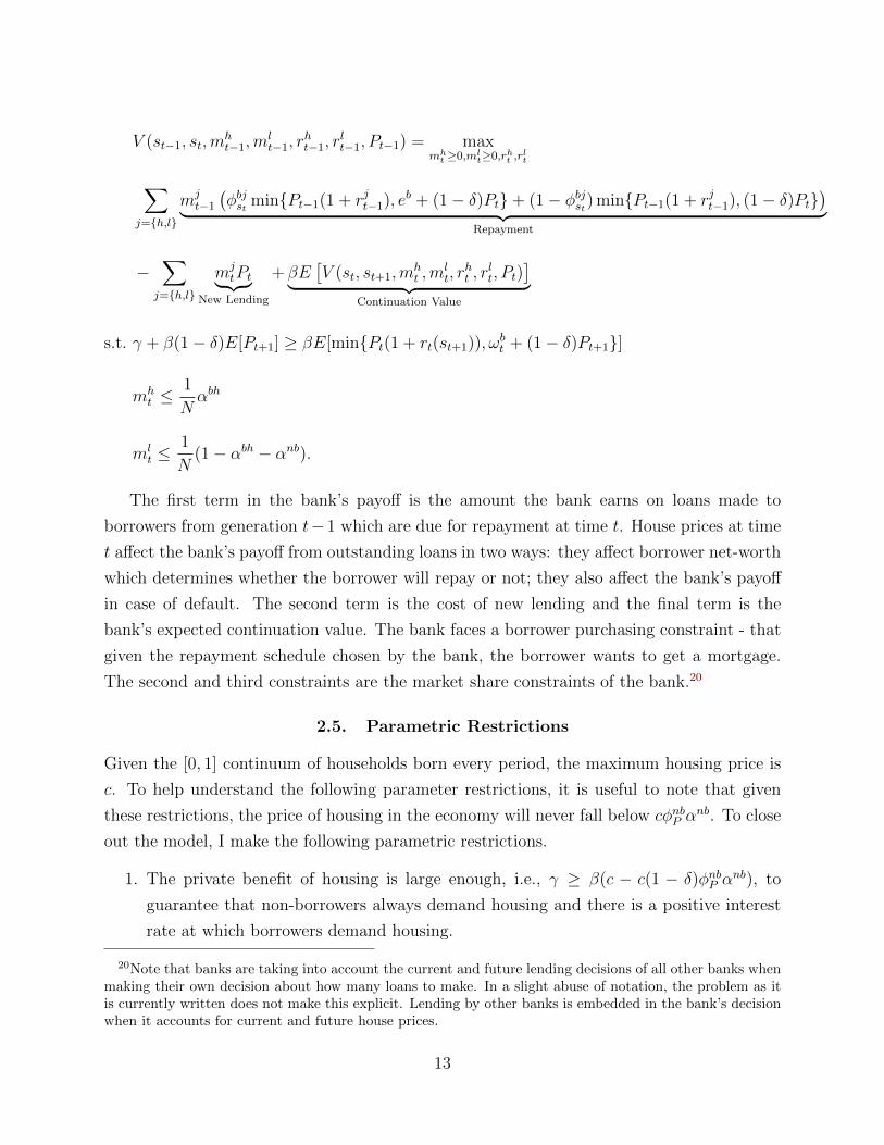
The first term in the bank’s payoff is the amount the bank earns on loans made to

borrowers from generation t−1 which are due for repayment at time t. House prices at time

t affect the bank’s payoff from outstanding loans in two ways: they affect borrower net-worth

which determines whether the borrower will repay or not; they also affect the bank’s payoff

in case of default. The second term is the cost of new lending and the final term is the

bank’s expected continuation value. The bank faces a borrower purchasing constraint - that

given the repayment schedule chosen by the bank, the borrower wants to get a mortgage.

The second and third constraints are the market share constraints of the bank.20

2.5. Parametric Restrictions

Given the [0, 1] continuum of households born every period, the maximum housing price is

c. To help understand the following parameter restrictions, it is useful to note that given

these restrictions, the price of housing in the economy will never fall below cφnbP αnb. To close

out the model, I make the following parametric restrictions.

1. The private benefit of housing is large enough, i.e., γ ≥ β(c − c(1 − δ)φnbP αnb), to

guarantee that non-borrowers always demand housing and there is a positive interest

rate at which borrowers demand housing.

20Note that banks are taking into account the current and future lending decisions of all other banks whenmaking their own decision about how many loans to make. In a slight abuse of notation, the problem as itis currently written does not make this explicit. Lending by other banks is embedded in the bank’s decisionwhen it accounts for current and future house prices.

13

2. Non-borrower endowment is large enough, i.e., enb ≥ c, to guarantee that a non-

borrower who receives a positive endowment can always afford to buy a house. Since

non-borrowers in the model are proxying for outside housing demand, this assumption

guarantees that credit is never the sole driver of house prices.21

3. In the theoretical results, depreciation is not too low, i.e φnbP αnb > 1− δ, to guarantee

that there is at least some new construction every period and that the bank’s problem

is thus continuous in house prices. In the calibrated version of the model, I do not

restrict the parameters to satisfy this assumption.

4. Low-quality borrower endowment is small enough, i.e.,

βφblReb + β(1− δ)c < cφnbP α

nb,

to guarantee that it is never profitable for banks to lend to low-quality borrowers. The

assumption on new construction every period guarantees that price never falls below

cφnbP αnb. This restriction helps to clarify the key mechanism of the model since for

any possible sequence of house prices and in any state, any mortgage loan made to

low-quality borrowers is NPV negative. Therefore, there is no reason a bank would

ever make loans to low-quality borrowers unless the return from propping up prices is

high enough.

Model Robustness: There are two key requirements for the results. First, house prices

affect a household’s ability or incentive to repay a mortgage such that higher housing prices

reduce the probability of default and/or the loss due to default. Second, credit provision has

an effect on house prices. The model is robust to modeling mortgage loans without recourse

and as fixed rate mortgages. The model is also robust to other market structures as long as

banks are able to make profits in one period and offset them with losses from another. The

model can also allow entry and exit so that banks lifetime profits are zero as long as they

can make profits or losses period-by-period.

3. Three-Period Model

To demonstrate the key mechanisms of the model I start by discussing the equilibrium in a

simplified three-period setting. This highlights how concentration affects both the quantity

and quality of credit. It also explains how, in concentrated markets, mortgage growth can

21This also helps simplify the model solution as house prices will always increase with more credit. Banksdo not crowd non-borrowers out of the market by making house prices too expensive.

14

be negatively correlated with income growth across areas and positively correlated with

income growth across borrowers. Uncertainty in future lending opportunities and intra-

period borrower heterogeneity are not necessary to obtain the key results of the model, and

therefore I abstract away from both in this simplified model. The full model keeps the

intuition of the three-period model and is additionally able to produce boom and bust cycles

with features that characterized the recent housing crisis.

In the first period the economy is in a rich-state with only non-borrowers and high-quality

borrowers, and in the second period a poor-state hits with certainty in which there are only

non-borrowers and low-quality borrowers. In the final period, no new generation is born

and therefore I assume the price of housing falls to an endogenously specified liquidation

value, cφnbP αnb ≥ κ ≥ 0. Since no high-quality borrowers are born in the second period, any

t = 2 lending will only be to low-quality borrowers. Since by assumption low-quality loans

are negative NPV, banks only lend a positive amount at t = 2 if they find it profitable to

prop up house prices. This setup thus clearly demonstrates when a bank is incentivized to

sacrifice loan quality for the return to keeping house prices high.22

I characterize the results of the model both when banks cannot commit to a level of t = 2

lending when making loans at t = 1 and when banks can commit to future lending. As I will

discuss, in both cases the results are qualitatively similar but the economic intuition for why

banks want to prop up prices is different. In practice, there are reasons to think that the

GSEs were able to commit, at least in part, to future lending. Hurst, Keys, Seru, and Vavra

(2016) provide evidence that the GSEs faced political pressure that did not allow them to

make substantial changes to interest rates. These constraints could credibly allow the GSEs

to commit to future activity.

The three-period model can be solved by backwards induction. Since no new generation

is born in the third period, banks do not lend at t = 3. In the second period, lending by any

given bank, m2 is stated in the following lemma, where M−i2 is lending by all other banks at

t = 2.

Lemma 1.A In the three-period model, without commitment to future lending, a bank’s

period-2 lending, m2, is given by the following two cases.

Case 1: If φbhR eb ≤ γ

β,

max

{0,m1(1− δ)

2− φnbP α +M−i

2

2+ β

φblP eb + (1− δ)κ

2c

}.

22In this three-period model, since t = 3 values are kappa and low-quality borrowers are only born att = 2, the fourth parametric restriction can be simplified to βφblP e

b + β(1− δ)κ < cφnbP αnb.

15

Case 2: If φbhR eb > γ

β,

max

{0,

(1− φbhR )m1(1− δ)2

− φnbP α +M−i2

2+ β

φblP eb + (1− δ)κ

2c

}.

In the three-period model, with commitment to future lending, a bank’s period-2 lending,

m2, is given by:

max

{0,m1(1− δ)

2− φnbP α +M−i

2

2+ β

φblP eb + (1− δ)κ

2c

}.

The loans a bank makes to low-quality borrowers, m2, is always increasing in outstanding

loans, m1. When m1 = 0 and the bank has no outstanding loans on its balance sheet, it

will never make any loans at t = 2 to low-quality borrowers and m2 = 0.23 As the amount

of outstanding loans increases, m2 can become positive. If at t = 1, a bank is unable to

commit to a level of future lending, m2, then it props up house prices to improve its return

on loans that are delinquent - when the borrower is unable to return the full face-value of the

loan. By increasing house prices through credit expansion, a bank is able to earn a higher

return on defaulting loans since it has a claim on the house. If a bank is able to commit to

future lending, it props up prices to improve its return on delinquent loans and additionally

to increase the face-value it can charge on non-delinquent loans. With commitment, a bank

therefore has greater incentives to prop up prices.24

Loans to low-quality borrowers, m2, is also increasing in the future expected income

of low-quality borrowers, φblP eb. It is decreasing in the housing demand coming from non-

borrowers and other banks, φnbP αnb +M−i

2 . A lower φnbP αnb +M−i

2 implies that an individual

bank effectively has larger market power in influencing house prices since outside sources of

demand are lower. In other words, a lower φnbP αnb +M−i

2 implies a larger elasticity of house

prices to credit.25. This increases the net benefit that credit expansion by the bank has on

house prices.

At t = 1, a bank takes into account its lending at time t = 2 when determining how

many loans to make. In period 1, a bank’s lending is stated in the following lemma, where

M−i1 is lending by all other banks at t = 1.

23Since low-quality loans are assumed to be negative NPV, −φnbP αnb −M−i2 + β

φblP e

b+(1−δ)κc < 0.

24When φbhR eb ≤ γ

β , bank lending at t = 2 is identical with and without commitment. In this case, t = 1

borrowers are willing to repay the bank φbhR eb + (1 − δ)P2 and by setting a face-value of the loan slightly

above this, banks can credibly raise house prices to improve their return on all outstanding loans at t = 2by propping up prices. For more detail on this, see the appendix.

25The elasticity of house prices is simply defined here as the percentage change in house prices for themarginal mortgage loan

16

Lemma 1.B In the three-period model, without commitment to future lending, a bank’s

period-1 lending, m1, is given by the following two cases.

Case 1: If φbhR eb ≤ γ

β,

m1 = max

{0,min

{βc

(φbhR e

b + (1− δ)P2

)− φnbR αnb −M−i

1

2,(1− αnb)

N

}}.

Case 2: If φbhR eb > γ

β,

m1 = max

0,min

βc

(γβ

+ (1− δ)P2

)− φnbR αnb −M−i

1

2−(β2(1− φbhR )φbhR (1− δ)2

).1{m2>0}

,(1− αnb)

N

.

In the three-period model, with commitment to future lending, a bank’s period-1 lending,

m1, is given by:

m1 = max

0,min

βc

(min{φbhR eb,

γβ}+ (1− δ)P2

)− φnbR αnb +M−i

1

2,(1− αnb)

N

.

In an equilibrium in which a bank props up house prices, if a bank lends more at t = 1, it

also increases its t = 2 lending. This pushes up housing prices at t = 2 (P2) in turn increasing

the amount of loans a bank makes at t = 1. There is thus a feedback loop between t = 1 and

t = 2 lending. Bank lending is also affected by the aggregate lending of other banks. The

number of loans a bank makes at t = 1 is decreasing in the number of loans made by other

banks, M−i1 , but increasing in the number of loans made by banks in the future, M−i

2 . The

more loans other banks make at t = 1, the higher is the price of housing at t = 1, making

it more expensive for a bank to make mortgage loans. This causes a bank to decrease the

amount it lends. The more loans other banks make at t = 2, the higher is the price of

housing at t = 2, allowing banks to charge a larger interest rate on loans made at t = 1

and increasing their incentive to lend at t = 1. There is thus strategic substitution in bank

lending within period but strategic complimenterities in bank lending across periods. The

full characterization of the equilibrium is discussed in the following subsection.

Numerical Example: To help understand the mechanism, I run through a numerical

example with N = 1. I choose the following parameters: αnb = .7, δ = .4, eb = $200, 000,

φbhR = 1, φblP = .7, κ = $100, 000, c = $300, 000. Following the second parametric restriction,

enb ≥ c. For simplicity, I assume no discounting, i.e. β = 1, and also have no non-borrower

income shocks, i.e. φnbR = φnbP = 1. I also assume γ ≥ φbhR eb, so that bank lending with and

17

without commitment are equivalent.26

Imagine a bank does not take into account the effect of house prices on the profitability

of its outstanding share of loans. Then in the second period, a bank will not prop-up prices.

It therefore makes makes no loans at t = 2 since all loans to low-quality borrowers are

negative NPV. Only non-borrowers will buy housing at t = 2. Therefore, housing demand

in the second period is hd2 = .7, and resulting house prices are chd2 = $210, 000. We can

check that loans to low-quality borrowers are negative NPV. House prices at t = 3 are given

by the liquidation value κ = $100, 000 and low-quality borrowers’ expected endowment is

φblP eb = $100, 000. If a bank was to lend to low-quality borrowers, it would have to pay

$210, 000 at t = 2 and receives an expected repayment of (1 − δ)κ + φblP eb = $200, 000 at

t = 3.

If a bank is not propping up house prices, it will make no loans in period 2. In the

first period, the bank will make m1 = .19 loans.27 Resulting house prices at t = 1, will be

chd1 = $268, 000. The cost of making t = 1 loans to a bank is $268, 000 and the expected

repayment from these loans is (1− δ)P2 +φbhR eb = $326, 000. The total profits earned by the

bank are .19 ∗ (326, 000− 268, 000) = $11, 213.

Now, let’s consider what happens if the bank takes into account its outstanding share of

loans in the second period and wants to deviate to making t = 2 loans. Then if the bank’s

outstanding share is m1 = .19, a bank will find it optimal to make m2 = .04 loans. This

will increase t = 2 price to $222, 400. The bank earns an increased return of $1, 438 on its

outstanding loans while making a loss of −$926 on new lending at t = 2. Banks are able to

make this gain in profits at the expense of young non-borrowers. They are harmed by this

increase in price and suffer an aggregate loss of αnb ∗ ($222, 400− $210, 000) = $8, 680. This

loss of young non-borrowers is transferred to banks, old non-borrowers, and construction

firms.

The increase in house prices at t = 2, allows banks to make a greater return per loan

they make at t = 1. Banks are now able to get an expected repayment of $333, 440 instead

of $326, 000. This makes banks want to lend more at t = 1. This will in turn make the

bank want to lend more at t = 2 and so on and so forth. Eventually, the bank will increase

t = 1 lending to .21 and t = 2 lending to .05. House prices at t = 2 will be $223, 516 and

at t = 1 will be $271, 720. The total profits earned by the banks make from t = 1 loans

is $12, 836 (an increase from $11, 213). The bank earns losses on t = 2 lending totaling

−$1, 059 which offsets some of these profits. Young non-borrowers at t = 2 account for the

26In this example, to guarantee that loans to low-quality borrowers are negative NPV, it is sufficient thatβφblP e

b + β(1− δ)κ < cφnbP αnb.

27Loan amounts can be calculated using Lemma 1.

18

rest of the transfer to banks.

3.1. Concentration and Credit

When concentration in mortgage holdings is low and each bank holds a small share of the

market, the return to propping up prices for any individual bank is low. Banks therefore

do not issue any loans to low-quality borrowers. As concentration increases, banks have

access to a larger share of high-quality borrowers at t = 1. In this case, they will issue loans

to risky borrowers to increase house prices and consequently the rents that they get from

high-quality borrowers. Formally, we can establish the following proposition,

Proposition 1 The three-period model has a unique equilibrium. There exists a cutoff, N ,

such that if N ≥ N , banks do not prop up houses prices and make no negative NPV loans. If

N < N , banks engage in risky lending to prop up house prices and supply a positive amount

of negative NPV loans.

When house prices at t = 2 are high, high-quality borrowers (who get a mortgage at t = 1)

make larger mortgage repayments to banks. This allows banks to earn greater rents from

them. As the market share of banks increases, they lend to more high-quality borrowers at

t = 1. This increases the effect of t = 2 house prices on their profitability. As concentration

increases, banks begin to make low-quality loans at t = 2 since credit expansion keeps house

prices high. As concentration decreases, banks begin to act more like price-takers in the

mortgage market and no longer make loans to prop up house prices.

Despite strategic complimenterities in bank lending across time, the equilibrium is unique.28

The uniqueness arises due to intra-temporal strategic substitution in bank lending. If other

banks pull back on lending at t = 2, an individual bank is incentivized to increase its own

lending at t = 2 and not cut back on its t = 1 lending enough to give arise to multiplicity.

There is therefore a unique equilibrium of the model.

As concentration increases aggregate credit can increase or decrease. There are two

competing effects. The first is a contemporaneous price effect. Large lenders internalize

their effect on house prices more than small lenders. The marginal increase in price when

making an additional loan affects large lenders’ cost of total lending more than that of small

lenders. Lenders in a concentrated market will therefore cut back on credit more than lenders

28Typically the presence of strategic complimenterities gives rise to multiple equilibria. The typical reasonfor multiplicity is as follows: when banks expect aggregate lending to be high at t = 2, they lend more att = 1, and the high t = 1 lending would lead to the high t = 2 lending that banks anticipated. Conversely,when banks expect lending at t = 2 to be low, they lend less at t = 1 which in turn leads to low t = 2 lendingas banks anticipated.

19

in a market with many small lenders. This effect is similar to a typical mechanism in Cournot

competition in which as concentration increases, the quantity of goods supplied on the market

decreases as suppliers internalize price effects more. As the number of banks decreases, this

“Cournot” effect leads to a decrease in credit supply. However, since concentration also

creates incentives to prop up prices, there is a second effect of change in concentration on

credit, the “propping-up” effect. Concentration increases banks’ incentives to increase t = 2

prices through credit expansion and if this effect is large enough, it can cause overall lending

to increase.

The following corollary summarizes the effect of concentration on mortgage lending:

Corollary 1 In the unique equilibrium of the three-period model, as N decreases,

1. credit extended by any given bank to both high- and low-quality borrowers increases,

2. if N ≥ N and banks are not propping up prices, aggregate credit decreases,

3. if N < N and banks are propping up prices, aggregate credit can increase.

When N ≥ N and banks are not propping up housing prices, aggregate credit is always

decreasing with concentration because of the Cournot effect. As is typical in most models

of competition, as the number of banks decreases, banks behave more like price-takers and

are willing to issue more loans. As discussed above, when N < N , there is a second effect of

concentration on credit, the propping-up effect. As banks acquire larger market shares, they

issue more loans per bank at t = 1. This increases the incentive for banks to prop up prices

and make negative NPV loans at t = 2. Higher t = 2 price further increase the incentive to

issue t = 1 loans and so on and so forth. As concentration increases, this feedback loop can

cause aggregate lending to increase.

Figure 1 illustrates the effect of concentration on house prices. It plots total credit,

measured as a sum of the number of households who get a mortgage at t = 1 and t = 2,

against the number of banks. As the market becomes more concentrated and the number

of banks decreases, banks begin to prop up house prices. In this parametrization, credit

increases with concentration in the region in which banks prop up prices, as the propping-up

effect dominates the Cournot effect. As concentration decreases and N > N , banks stop

propping up prices and the amount of credit increases as competition in the market causes

banks to behave more and more like price-takers.

20

Figure 1: The figure above plots total credit, measured by the number of households who get a mortgage,against the level of concentration in the mortgage market. As we move along the x-axis, N increases andconcentration decreases. The parametrization is as follows: δ = .01, αnb = .2, φblP = .2, φbhR = 1, φnbP = .7,φnbR = 1, eb = 2 ,κ = .45, γ = 4, c = 9.8.

Looking at Figure 1, we can see that it is possible for two areas with different levels of

concentration to have the same amount of aggregate credit. However, the composition of

this credit is different. In particular, the credit in the area with larger concentration is riskier

- a larger fraction of lending is to high-risk borrowers. Figure 2 overlays the first graph with

different credit risk characteristics - debt-to-income ratios and default rates.

As Figure 2 illustrates, although two areas with differing concentration can have the same

aggregate credit, the credit in the area with higher concentration is riskier. When banks are

propping up prices, they extend credit to riskier households with high default rates and make

negative NPV mortgage loans. If there is an economic cost to high mortgage default rates,

this result suggests that a safer way to expand homeownership would be through increased

competition rather than through creating agencies that concentrate mortgage risk. This may

however come at the cost of lower income (and negative NPV) households not getting credit.

21

Figure 2: The figures above plot the debt-to-income ratio and default rates on the right y-axis againstconcentration. As we move along the x-axis, N increases and concentration decreases. The parametrizationis as follows: δ = .01, αnb = .2, φblP = .2, φbhR = 1, φnbP = .7, φnbR = 1, eb = 2 ,κ = .45, γ = 4, c = 9.8.

3.1.1. The Effect of Various Model Primitives

A number of factors affect banks’ incentives to prop up house prices. When the expected

income of low-quality borrowers, φblP eb, is high it is relatively more profitable to lend to

low-quality borrowers and banks have to take a smaller loss on these loans in their effort

to prop up prices. Therefore this increases the incentive to prop up house prices. When

non-borrower income growth in the poor state, φnbP , is low banks have relatively more market

power when it comes to affecting house prices, increasing the incentive to prop up prices.

Finally, when δ is low, houses are worth more in future periods increasing how much banks

and households value the future asset value of a house. As banks are incentivized to prop up

prices more when these primitives change, the threshold level of concentration necessary for

banks to make high-risk loans decreases. The following corollary formalizes how N changes

with the various primitives of the model.

Corollary 2 In the three-period model, N increases as the expected income of low-quality

borrowers increases, as the depreciation rate decreases, and as non-borrower growth in the

poor state decreases. Formally,

∂N

∂φblP eb> 0,

∂N

∂δ< 0 and

∂N

∂φnbP< 0.

3.1.2. Asset Value of Housing

The key property of housing that gives rise to this mechanism is that housing is a durable

asset with future value. This is distinct from other goods that only serve a consumption

22

purpose. When δ = 1 and housing depreciates completely, banks and households do not care

about future house prices. There are no incentives to prop-up prices, and only the Cournot

effect remains. As δ decreases, the asset value of the house increases, causing banks and

households to value future house prices. This creates an incentive to prop up prices when

banks have a large enough exposure to the housing market. At low values of δ, the incentives

to prop up prices is stronger since housing is worth more upon repayment leading to a higher

value of N . Lower values of δ also increases household net worth upon repayment and allow

banks to charge larger repayments from households when making mortgage loans increasing

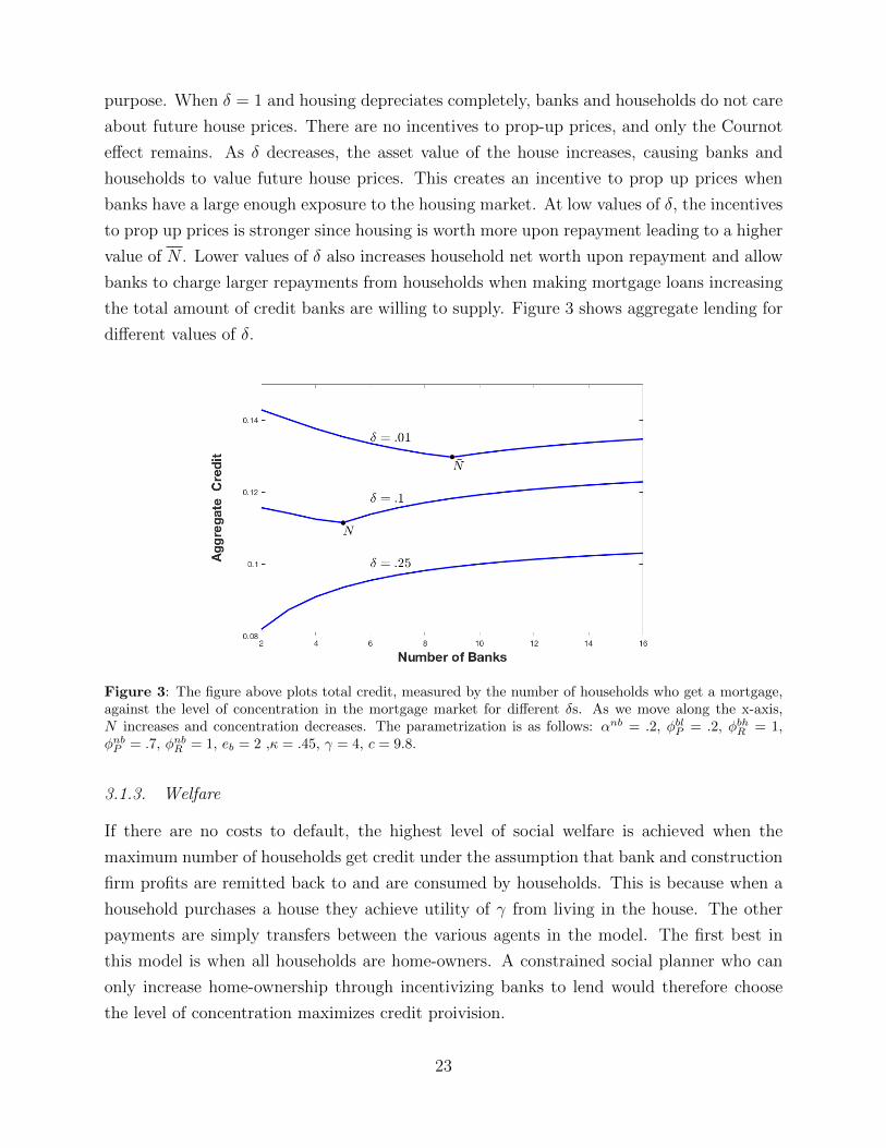
the total amount of credit banks are willing to supply. Figure 3 shows aggregate lending for

different values of δ.

Figure 3: The figure above plots total credit, measured by the number of households who get a mortgage,against the level of concentration in the mortgage market for different δs. As we move along the x-axis,N increases and concentration decreases. The parametrization is as follows: αnb = .2, φblP = .2, φbhR = 1,φnbP = .7, φnbR = 1, eb = 2 ,κ = .45, γ = 4, c = 9.8.

3.1.3. Welfare

If there are no costs to default, the highest level of social welfare is achieved when the

maximum number of households get credit under the assumption that bank and construction

firm profits are remitted back to and are consumed by households. This is because when a

household purchases a house they achieve utility of γ from living in the house. The other

payments are simply transfers between the various agents in the model. The first best in

this model is when all households are home-owners. A constrained social planner who can

only increase home-ownership through incentivizing banks to lend would therefore choose

the level of concentration maximizes credit proivision.

23

We can add default costs to the model by assuming some deadweight losses per default d

which are not internalized by banks or households. These costs are social costs in the sense

that they are not internalized by banks or households and destroy the end-of-period utility

of all households equally. We can imagine these costs are part of the net profits remitted to

households at the end of the period. If there are social costs to default, then if an increase in

concentration increases credit, this improves welfare if the net gain in utility by households

from consuming housing is higher than the deadweight losses due to default.

Recall from Figure 1, that it is possible to achieve the same level of aggregate credit for

two different levels of concentration. An important welfare insight of the model is that in

such a case, given any non-zero default costs, welfare is always higher in the area with lower

concentration. Formally,

Proposition 2 Let d be social costs of default. If ∃ N1 < N ≤ N2 s.t. the total number of

households with access to credit is equal under both N1 and N2, then for any d > 0, aggregate

welfare is higher under N2 than N1.

This proposition is quite powerful because it is saying that for a large set of parameters,

it is optimum to increase competition and decrease concentration as long as there are any

costs to society of mortgage defaults, however small or large these costs might be. In this

case, the constrained social planner will always choose N2. The recent crisis has highlighted

that there can be large costs to mortgage defaults, and in that context this model would

generally advocate for a reduction in concentration.

3.2. Mortgage Growth and Income Growth

There has been an active debate on whether the housing boom and bust was driven by

a supply shock or by expectations of high future house prices. Much of this debate has

revolved around understanding the relationship between income growth and credit growth

during the housing boom. In support of the first hypothesis, Mian and Sufi (2009) find

that income growth decoupled from the growth in mortgage credit in the U.S. at the ZIP

code level. They stress that such a result is in line with the supply shock hypothesis since

lending seemed to have increased disproportionately to borrowers at the lower end of the

income distribution. In a paper, looking at more micro borrower-level data Adelino et al.

(2016) find that income and mortgage credit growth remained positively correlated at the

borrower-level. They argue that this is more in line with high house price expectations since

credit increased across the income distribution and was not disproportionately extended to

high-risk low-quality borrowers.

24

The model can simultaneously produce different correlations between income growth

and the growth in mortgage credit when looking at borrower-level data versus data that is

aggregated (eg. to a ZIP code level). In the model, an exogenous increase in concentration

can cause a credit-supply shock that propagates through the expectation of higher future

house prices as large lenders have an incentive to prop up house prices. This can generate a

negative correlation between the growth in mortgage credit and income growth across areas

(eg. across ZIP codes) while still maintaining a positive correlation between the two at a

borrower-level. Specifically, consider a change in concentration when the number of banks

decreases from N1 > N to N2 < N such that banks move from not propping up prices at

t = 2 to propping up prices. Define ∆M as the change in mortgage credit following this

increase in concentration. Then, we can establish the following proposition,

Proposition 3 Following an increase in concentration when the number of banks decreases

from N1 ≥ N to N2 < N and banks begin to prop up house prices, mortgage credit growth

is negatively correlated with non-borrower income growth in the poor state and positively

correlated with borrower income growth in the poor state i.e,

∂∆M

φnbP< 0, and

∂∆M

φblP> 0.

As concentration increases the magnitude of the credit supply shock is largest in areas

that have the lowest growth in non-borrower income.29 All else equal, when non-borrower

income growth is low at t = 2 , the intra-period strategic substitution effect leads banks

to extend more credit. In the absence of other sources of demand to drive up housing

prices, the effective market power of banks in the housing market is higher. As a result, for

every additional mortgage loan that banks extend to low-quality borrowers, the percentage

increase in housing prices is greater when non-borrower income growth is low. The returns

to propping up prices are therefore highest in areas with low-income growth. Looking at

borrower-level income growth, the return from making mortgage loans to borrowers is higher

when borrowers have larger expected income growth. All else equal, a bank would always

prefer to make a loan to a high-quality borrower, if possible, as such a loan would also serve

to increase house prices. The growth in mortgage credit is therefore positively correlated to

the growth in borrower income, φb.

Following an exogenous increase in concentration, this negative correlation between non-

borrower income and mortgage credit growth can cause areas with low-income growth to

experience larger credit-supply shocks than areas with higher income growth. Figure 4

29Note that since N depends on φblP and φnbP , this proposition only compares areas given an N1 and N2

s.t. N for each area falls within (N1, N2].

25

Figure 4: The figure above plots total credit, measured by the number of households who get a mortgage,against the level of concentration in the mortgage market for different income growths between t = 1 andt = 2. As we move along the x-axis, N increases and concentration decreases. The parametrization is asfollows: δ = .01, αnb = .2, φblP = .2, φbhR = 1, φnbR = 1, eb = 2 ,κ = .45, γ = 4, c = 9.8. φnbP is varied to getchanges in income growth across the two plots - it is equal to .73 is the high-income growth area and .7 inthe low-income growth area.

illustrates such a case by plotting aggregate credit across an area with high versus low

income growth. In the region in which banks do not prop up prices, mortgage credit growth

is positively correlated to income growth. Banks only consider the return they make on the

mortgage loan itself, which increases when income growth is higher. When the mortgage

market is concentrated and banks are propping up prices, it is possible for credit to be higher

in areas with relatively low-income growth as the return to propping up prices is higher in

areas with low non-borrower income growth. In the example in Figure 4, imagine an increase

in concentration which causes the number of banks to go from 8 to 6. In this case, the area

with high-income growth will experience a decline in credit due to decreased competition

amongst banks. At the same time, the area with low-income growth will experience a positive

growth in credit due to an increase in the market power of banks.

At the borrower-level, the growth in mortgage credit and income growth can remain

positively correlated. In the simplified three-period model, I provide the intuition for

this result but do not show it explicitly as there is no inter-period heterogeneity amongst

borrowers. Appendix B outlines an example with inter-period borrower heterogeneity that

shows how the model can simultaneously produce a negative correlation between credit

growth and income growth amongst areas (such as ZIP codes) which maintaining a positive

correlation at the borrower-level.

26

Note that the empirical facts are not unequivocally agreed upon.30 It is outside the

scope and not the goal of this paper to take a stance on what empirical facts are valid and

whether in fact income and mortgage credit did or did not decouple across ZIP codes and

across borrowers. Therefore, the paper cannot claim to explain the behavior of income and

mortgage credit growth during the crisis as the empirical agreement on these facts has yet

to be fully reached. Rather this paper is concerned with how we interpret these correlations

by providing a theoretical basis for understanding these correlations and how their meanings

can differ depending on the level of data aggregation.

In the three-period model, by construction in the last period house prices fall to κ

demonstrating that banks may lend to low-quality borrowers even if a crash in house prices

is inevitable. This helps illustrate the incentives banks have to prop up prices in the simplest

possible setup. In the infinite horizon model in Section 4, we get more realistic price processes

for housing prices and credit and can assess how concentration can lead to credit booms and

busts in house prices.

4. Infinite Horizon Model

I now solve the infinite-horizon model which gives rise to boom and bust cycles that can

explain various empirical facts that defined the housing crisis. In the full model, there is intra-

period heterogeneity: each period has both high- and low-quality borrowers. Additionally,

there is uncertainty about the state of the world: with probability q a rich generation is born

and with probability 1 − q a poor generation is born in which all households have a lower

expected income.

The path dependency of this problem can make it complicated to solve since in every

state banks have to decide how much to lend taking into account outstanding loans and

future lending. Furthermore, they also have to account for how the lending decisions of

other banks will affect both current and future house prices. Given the model setup, it

is possible to simplify a bank’s maximization in a similar way as the three-period model

to get a tractable problem.31 In the infinite horizon model, we can show that similar to

the model with three periods, once markets become concentrated banks have incentives to

prop up house prices. Furthermore, because of intra-period strategic substitution amongst

banks, the economy has a unique equilibrium despite strategic complimenterities in lending

across periods. Initialize initial loans to 0. Then we can establish the following proposition

analogous to the three-period case,

30See Mian and Sufi (2016), Mian and Sufi (2015) and Adelino et al. (2015)

31Details are provided in the appendix.

27

Proposition 4 The infinite-horizon model has a unique equilibrium. There exists a cutoff,

N , such that if N ≥ N , for any possible sequence of shocks, banks do not make any loans

to high-risk, low-quality borrowers to prop up prices. If N < N , there are a strictly positive

number of sequences of shocks in which banks will extend credit to high-risk, low-quality

borrowers to prop up house prices.

The key intuition for this proposition is identical to that in the three-period case. When

N is large, each individual bank has a small amount of loans on its books. Therefore banks

do not benefit from making loans that are unprofitable to push up house prices as the return

from propping up prices is low. As N increases and individual banks acquire larger market

shares, increasing house prices allows them to profit from a greater number of loans. This

increases the return from keeping house prices high. Therefore, as concentration increases,

the equilibrium begins to feature loans that are made to high-risk borrowers even if the loan

itself is negative NPV.

An important feature of the equilibrium is that conditional on the state of the economy,

lending per bank is increasing in its outstanding loans. Formally,

Corollary 3 Conditional on the state of the economy, aggregate lending, Mt, is increasing

in aggregate outstanding loans, Mt−1. Lending per bank, mt, is similarly increasing in

outstanding loans, mt−1, conditional on the state of the economy.

This feature of the equilibrium naturally generates housing boom and bust cycles and is

discussed in the remainder of this section.

4.1. Boom and Bust Cycles

An exogenous increase in concentration can lead to credit booms and busts with features

that match key empirical facts about the recent housing crisis.

Credit Boom, Rising House Prices and Rising DTI Ratios: In the equilibrium,

the amount of loans a bank makes is increasing in the its outstanding loans, conditional on the

state of the economy. This feature of the equilibrium naturally gives rise to an increasing

time-series of credit and house prices following a series of positive income shocks.32 This

increase in credit happens even though the “fundamentals” of the shock, the underlying

income of households, stays the same. The increase in credit is rather driven by the fact that

32For example, imagine that all banks start with 0 loans on their books and at t = 1 a high shock occursand banks make m1 > 0 loans. Then at t = 2 banks have m1 > 0 loans outstanding on their books. If att = 2 another high shock occurs, given that mt is increasing in mt−1 conditional on the state of the economy,m2 > m1. And so on and so forth for any consecutive high shocks.

28

R R R R P P

States0.48

0.52

0.56

0.6

0.64

Aggr

egat

e Cr

edit

High Concentration: N=2Low Concentration: N=4

Figure 5: The figure above plots total credit, measured by the number of households who get a mortgage,across two areas with different concentration for a series of income-shocks on the x-axis. Details of theparametrization are in Appendix C.

lenders find it profitable to increase credit expansion to prop up house prices as the size of

their outstanding exposure to the mortgage market increases. This effect is most pronounced

for lenders with access to a large number of potential borrowers since they make more loans

per bank, increasing the incentive to prop up prices in subsequent periods. Furthermore,

they are able to make a larger number of mortgages before being limited by the market

share constraint. They are therefore able to acquire larger and larger mortgage exposures,

increasing their incentive to prop up prices. High concentration can therefore cause credit

booms to be much larger than when concentration is low. Since the fundamentals of the

economy in terms of expected borrower income remain the same, the only thing that is

changing over time are house prices driven by greater credit expansion. The credit boom is

therefore accompanied by an increase in house prices and rising debt to income ratios.

Figure 5 shows how a credit boom and bust differ in high concentration versus low

concentration areas in an economy that has a series of consecutive high shocks followed by

low shocks. In this example, the area with a higher concentration has approximately 25%

more credit expanded at the height of the boom than the area with low concentration.

Rise in Risky Lending: The recent housing crisis had an unprecedented increase in

risky lending with mortgages being extended to borrowers with low FICO scores at high

DTI and LTV ratios. Figure 6 shows the composition of credit during the boom and bust

cycle. The right y-axis plots the percentage of credit extended to low-quality borrowers

in the credit boom. Not only do areas with high concentration have larger credit booms,

29

R R R R P P

States0.48

0.52

0.56

0.6

0.64

Aggr

egat

e C

redi

t

0

0.1

0.2

0.3

0.4

0.5

Perc

enta

ge L

ow-Q

ualit

y

High Concentration: N=2Low Concentration: N=4

Figure 6: The bars in the figure above plot the percentage of loans (right y-axis) made to high-risk, low-quality borrowers across two areas with different concentration for a series of income-shocks on the x-axis.The lines plot total credit (left y-axis), measured by the number of households who get a mortgage. Detailsof the parametrization are in Appendix C.

the composition of that credit is riskier. Also note that there is a boom in credit to high-

quality borrowers during rich-shocks in both high- and low- concentration areas. This is

by virtue of fundamentals being better during high shocks and is in line with findings by

Adelino et al. (2016) that credit expansion increased across the income distribution during

the credit boom. However, the increase in outstanding loans in high concentration areas

also creates an incentive to prop up prices, leading to loans additionally being made to low-

quality borrowers. The overall composition of credit is therefore riskier in high concentration

areas during credit booms.

Timing of Risky Lending during Boom: The rise of risky lending happened in the

early- to mid-2000s even though house prices had been rising since the 1990s. Most theories

on the rise of risky lending do not account for the timing of the rise. For example, the

securitization of mortgages was common since the 1990s but the rise in risky lending was

not observed until later. As Figure 6 illustrates, the amount of risky lending increases over

the life of the credit boom and does not start immediately on entering a rich state. Since

low-quality loans are negative NPV, lending to risky borrowers is profitable only when the

return from propping up house prices is high. A lender’s portfolio needs to be large enough

for there to be an incentive to make risky loans. Since the number of outstanding loans

increases over the life of the boom, high-risk lending will begin after the start of the boom

once the outstanding mortgage exposure is large enough. The exact timing of the start of

risky lending depends on the amount of concentration and the profitability of high- and

30

low-quality loans. As banks are incentivized to prop up prices, they will first saturate the

high-quality market and only then move on to riskier lending.

Continuation of Risky Lending after Boom: Lastly, Figure 6 illustrates that once a

low-shock hits the economy, lenders in the highly concentrated area continue to make risky

loans for a short time. Even though fundamentals in a poor state worsen, since large lenders

have a lot of outstanding loans, they have an incentive to keep lending to keep house prices

high. Essentially, large lenders react less to fundamental shocks than small lenders because

of the size of their balance sheet. In recent work, Elul et al. (2017) find that the GSEs

increased their risky activity in 2007 when markets began to slow down and when private

securitizers started withdrawing from the market. Further, this increase happened in MSAs

in which the GSEs had a large outstanding share. Additionally, Bhutta and Keys (2017)

find that private mortgage insurance issuance which allowed the GSEs to securitize loans

with riskier fundamentals also increased in 2007 as the housing market was beginning its

downturn. Both papers also find that this seemed to be happening in areas where other

players were pulling out of markets. As house prices are likely to fall when other sources of

housing demand slow down, this is in line with my model predictions.

The model thus explains many facts about the recent housing crisis. As discussed earlier,

when Salomon Brothers got investors interested in MBS as an investment vehicle, Fannie

Mae and Freddie Mac grew their market share tremendously having a monopoly on prime

securitization and later became the biggest investors in private label MBS. This event can

be viewed as an exogenous increase to the GSEs market power, giving them access to large

share of potential borrowers. The model can help us understand the credit boom and bust

following this increase in GSE market power. Moreover, the model can explain cross-sectional

patterns in GSE lending which can help explain why they continued to make risky loans in

MSAs in which they had a high outstanding share.

5. Extensions

This section discusses some extensions to establish some additional results and robustness

of the model mechanism.

5.0.1. Secondary Market Equivalency

During the housing boom, there was a large concentration in mortgage holdings at the GSE

level and amongst a few large banks who purchased many MBS. In the model described

so far, mortgage originators are assumed to be the final holders of these mortgages. The

baseline model can be reframed as an equivalent problem in which mortgage holders purchase

31

mortgages from a secondary market and do not originate any loans themselves. The key

mechanism works as long as there is concentration in mortgage holdings at some level and

agents with exposure to mortgage payments have some market power. If secondary market

players own a large share of the mortgage market, they want to keep house prices up. If they

have market power, they can offer attractive prices on the secondary market for sub-prime

mortgages that will incentivize mortgage originators to issue mortgages to risky borrowers.

Holders of these mortgages will suffer losses on these risky purchases but the increase in

house prices will be profitable for their outstanding mortgage exposure.

The equivalent model is as follows. A continuum [0, 1 − αnb] of banks competitively

originate mortgages and sell them to a secondary market. Each bank has access to one

borrower in the continuum of borrowers. Final mortgage holders purchase mortgages on the

secondary market from originators. Each holder has access to a fraction 1N

of originators and

thereby to a fraction 1N

of borrowers. Assuming mortgage originators follow an originate-to-

distribute model and do not hold mortgages is equivalent to assuming that their main source

of funding comes from secondary markets. The originate-to-distribute model was common

amongst mortgage originators during the housing boom (Purnanandam (2011)). Loutskina

and Strahan (2009) and An and Yao (2016) provide evidence that the GSEs were a key

source of liquidity provision for non-jumbo loans issued by banks.

A bank that originates mortgages is offered a secondary market price, Yt(rjt , ω

bjt ), for a

mortgage originated at time t to a household j with expected endowment ωbjt at interest rate

rjt . An originator will make a mortgage loan to a borrower if:

Yt(rjt , ω

bjt )− Pt ≥ 0.

Each period holders of mortgages will choose to post secondary market prices taking

into account their effect on originator decisions and how that influences housing prices.

I assume that secondary market holders can purchase mortgages at different rates from

different mortgage originators thereby allowing them to control how many mortgages of a

type they wish to purchase. Therefore, secondary market mortgage holders maximize the

following, where mjt−1 is the number of mortgages of type j{h, l} they purchased in the

previous period,

32

V (st, st−1mht−1,m

lt−1, r

ht−1, r

lt−1, Pt−1) = max

mht ≥0,mlt≥0,Y jt ,Ylt ,r

mt ,r

lt∑

j={h,l}

mjt−1

(φbjst min{Pt−1(1 + rjt−1), eb + (1− δ)Pt}+ (1− φbjst) min{Pt−1(1 + rjt−1), (1− δ)Pt}

)︸ ︷︷ ︸Repayment

−∑

j={h,l}

mjtY

jt︸ ︷︷ ︸

New Lending

+ βE[V (st+1,m

ht ,m

lt, r

ht , r

lt, Pt, st)

]︸ ︷︷ ︸Continuation Value

s.t. Yt(rjt , ω

bjt )− Pt ≥ 0

γ + β(1− δ)E[Pt+1] ≥ βE[min{Pt(1 + rt(st+1)), ωbt + (1− δ)Pt+1}]

mht ≤

1

Nαbh

mlt ≤

1

N(1− αbh − αnb).

The mortgage holder will pick Yt so that the originator is just willing to lend, implying

that Yt = Pt. Furthermore, they will choose an rt so that borrowers repay the maximum

they are willing to pay. This is equivalent to the problem faced by banks that hold onto

the mortgages they originate. The same logic can be applied if mortgages are resold on the

secondary market. The key requirement for the mechanism to work is that the final holder

of mortgages has some market power.

5.0.2. Refinancing

Since the model has one-period mortgage contracts, it abstracts away from the bank choosing

to refinance mortgage contracts to prevent defaults instead of issuing new mortgage loans.

Trivially, in the model if the bank could simply give an existing borrower who is due to repay

their mortgage loan a new mortgage this would be equal to writing down their debt to a

face-value of zero (the endowment in the low state). In this case, it is possible to show that

making a new borrower a mortgage loan rather than refinancing the existing mortgage is

always a dominant strategy as the bank can additionally harness the new borrower’s expected

endowment. If it is not possible to make loans to new borrowers, the same intuition for

propping up prices applies and a bank will be willing to make a negative NPV refinancing

loan if it has large enough outstanding mortgage exposure.

The baseline three-period model can be extended to incorporate the possibility of refinancing

33

in a less trivial way. We can modify the model and assume that the generation born in period-

1 lives for three periods and gets utility from consumption in either the second or the third

period. The generation born at t = 1 therefore gets utility,

u(k1, c2, c3) = γk1 + βc2 + β2c3

At t = 2, if a household from generation 1 gets an endowment of 0, with probability φbRPthey will receive an income of eb at t = 3. This captures the idea that some households may

have delayed income. At t = 2, a bank can either choose to make a new loan to prevent

defaults, or to refinance defaulting borrowers and issue them a new mortgage instead. For

simplicity, I assume that since the mortgage loan has recourse, a borrower who is in default

has to accept the bank’s refinancing offer at t = 2 if the new payment demanded does not

exceed the face-value of the loan multiplied by the discount factor β. In this case, a bank

would prefer to refinance an existing borrower rather than lend to prop up prices to a new

borrower if,

φbRP > φbP

If φbRP < φbP a bank would strictly prefer to make new loans rather than refinance existing

borrowers. The intuition for this is relatively straightforward. The bank will simply go for

whichever option is less negative NPV. This will depend on whether a loan to a new bad-

quality borrower or the existing borrower in default has higher expected future repayment.

The basic intuition is applicable to both refinancing and new loans. In line with this, Elul

et al. (2017) find that the GSEs were more likely to make both high LTV refinancing and

purchase loans in areas where they had large outstanding exposure.

5.0.3. Lender Heterogeneity: Large and Small Lenders

During the housing boom and bust, while the GSEs and some large LCFIs acquired a large

share of the mortgage market, there were also smaller mortgage market participants. The

model can be extended to evaluate the case of some large lenders and many small, dispersed

lenders who behave like price-takers in the mortgage market. Specifically, I modify the model

to allow small, dispersed lenders to have access to a share s of households while large lenders

have access to the remaining ones.

The previous results and intuition all apply here. Furthermore, in a boom-bust cycle,

following a series of h shocks, the effective market share of a large lender as measured by the

percentage share of all mortgages held by that lender over the total number of mortgages

outstanding, is increasing over time even though access to borrowers stays the same. This is

34

because as a large lender acquires more outstanding mortgages over the boom, the incentive

to prop up prices increases, leading the lender to increase credit. This effect is not present for

small lenders who are price-takers. The exposure of the large lender to the total mortgage

market therefore increases over time. This extension of the model matches the empirically

observed increase in Fannie Mae and Freddie Mac’s market share over the housing boom.

I also calibrate this extended model to U.S. data. The calibration is discussed in section

6.1. As concentration increases, the size of the credit boom and extension of risky credit also

increase. Importantly, now the market share of large lenders increases over the boom. Figure

7 shows a credit boom and busts in areas with differing concentration. It also shows that

the gain in effective market share of a large lender is lower when there are more competing

lenders.33

Figure 7: The panel on the right above plots the total amount of credit extended, measured by the number ofhouseholds who get a mortgage loan on the y-axis and the percentage of loans made to high-risk, low-qualityborrowers, on the right y-axis, across two areas with different concentration for a series of income-shockson the x-axis. The panel on the left shows the effective market share of large lenders across two areas withdifferent concentration for a series of income-shocks on the x-axis. Details of the parametrization are inAppendix C.

6. Calibration Exercise

I now calibrate the stylized model to the U.S. economy. The main purpose of this model is

to clearly illustrate the theory of how concentration in the mortgage market can create an

incentive to extend risky credit to keep house prices high and how that can produce credit

cycles with dynamics similar to that of the recent housing crisis. In doing so, the model

33This version of the calibration has the market share of large lenders decreasing upon the bust. Theeffective market share may also increase if non-borrower demand and the provision of mortgages by smallprice-taking lenders slows down.

35

abstracts away from various aspects of mortgage markets, housing decisions by households,

details of mortgage contracts, etc. A deeper examination of the quantitative implications

of concentration on mortgage credit requires a more detailed quantitative model. However,

this calibration of the stylized model can help us address two questions. First, does the

model produce quantitatively significant credit and house price dynamics that match the

U.S. experience in the recent housing crisis? Second, does simply changing the level of

concentration produce significant variation in the path of credit and house prices? If the

answers to these questions are positive, then it provides support for this paper’s theory that

the housing boom and bust was driven by a change in concentration.

The model is calibrated to to the 1991-2009 U.S. housing market with the boom quantities

aggregated across 1991-2006 and the bust quantities aggregated across 2007-2008. For this

exercise, I assume that the economy experienced a sequence of rich shocks in the boom years

followed by a sequence of poor shocks in the bust years. The rich and poor shocks are mapped

to Federal Reserve Economic Data on the growth rate of personal income. From 1991-2006

real median personal income growth at an annual rate of 1.5% while from 2007-2009 it grew

at an annual rate of -1.6%. Appendix C provides a detailed description of the data.34

Table 4 in Appendix C summarizes the benchmark configuration of the model parameters.

Here, I discuss the parameters and results when calibrating the model with lender heterogeneity

as that allows me to better target the GSE share of the mortgage market. As I lack data on

the exact market share of LCFIs, I do not attempt to capture their share in the calibration.

I choose s=.6 and N = 2 to roughly match the GSEs’ eventual market share at the height of

the boom. The income shocks of high- and low-quality borrowers in the rich- and poor-states

of the economy are chosen to match the default rates on prime and sub-prime loans during

the boom and bust. The fraction of high-quality borrowers is chosen to match the fraction

of prime versus sub-prime lending while the fraction of non-borrowers is chosen to match the

fraction of cash-only house purchases.

Table 5 in Appendix C compares the model-generated quantities for the calibration to

those in the data. A one-time change in concentration is able to match the house price

increase and decrease well, explaining approximately 45% of the boom in house prices. A

fundamental shock to the concentrated market explains about 30% of the bust in house prices.

It also does a good job of matching the fraction of sub-prime borrowers during the boom

explaining over 90% of the lending to sub-prime borrowers in the boom but overestimates the

lending to sub-prime borrowers slightly during the bust. This may be partially driven by the

fact that during 2007, the GSEs kept lending to high-risk borrowers but private securitizers

34Appendix C tables 1-3 also provide results for calibration of the benchmark model without lenderheterogeneity.

36

started pulling out of the high-risk market.

Table 6 in Appendix C does a counterfactual analysis. I decrease concentration by

doubling N from 2 to 4 while keeping the other parameters of the benchmark calibration the

same. This change in concentration decreases the fraction of sub-prime lending in the boom

to 0 in both the boom and bust. The boom also has 30% lower growth in house prices while

the bust has about 80% smaller decline in house prices.

The model can therefore produce quantitatively meaningful magnitudes and changes

in credit and prices when looking at the housing boom and bust. Moreover, changing

concentration can result in significant changes to the model-implied credit boom and bust.

This suggests that concentration can be an important channel that contributes to credit

cycles and a more comprehensive quantitative exploration of this channel is interesting for

future research.

Conclusion

This paper provides a novel theory of how concentration in mortgage markets can affect both

the quantity and the quality of mortgage credit. Lenders with a large outstanding mortgage

exposure have incentives to extend risky credit to prop-up house prices. An increase in

concentration in mortgage markets can generate housing booms and busts with features

that match the recent U.S. housing crisis.

In the aftermath of the housing crisis, policy makers have wanted to design policy to

curb high-risk lending. However, the role that concentration can play in creating incentives

to extend risky mortgage credit has been largely overlooked in this process. The Economist

recently reported that concentration in mortgage markets has increased since the crisis as a

side-effect of new regulations faced by banks which have made them move out of mortgage

lending. Somewhat ironically, many of these regulations are intended to reduce risky lending.

The GSEs and the FHA are currently funding between 65-80% of new mortgages, many

of which appear to be highly risky. A fifth of all loans since 2012 have LTV ratios of

over 95%. This is comparable to the fraction of sub-prime lending in the years before the

housing collapse. As this paper demonstrates, such high concentration can have a significant

impact on both the quantity and quality of credit. It is therefore crucial to comprehensively

understand the different forces that incentivize high-risk lending when designing policy.

37

References

Acharya, V. V., M. Richardson, S. V. Nieuwerburgh, and L. J. White (2011). Guaranteed to

Fail: Fannie Mae, Freddie Mac and the Debacle of Mortgage Finance.

Adelino, M., W. S. Frame, and K. S. Gerardi (2016). The Effect of Large Investors on Asset

Quality: Evidence from Subprime Mortgage Securities. Working Paper .

Adelino, M., A. Schoar, and F. Severino (2015). Loan Originations and Defaults in the

Mortgage Crisis: Further Evidence. Working Paper .

Adelino, M., A. Schoar, and F. Severino (2016). Loan Originations and Defaults in the

Mortgage Crisis: The Role of the Middle Class. The Review of Financial Studies 29 (7),

1635–1670.

Agarwal, S., G. Amromin, S. Chomsisengphet, T. Landvoigt, T. Piskorski, A. Seru, and

V. Yao (2017). Mortgage Refinancing , Consumer Spending, and Competition : Evidence

from the Home Affordable Refinancing Program Abstract. Working Paper .

Amel, D. F., A. B. Kennickell, and K. B. Moore (2008). Banking Market Definition: Evidence

from the Survey of Consumer Finances. Working Paper .

An, X. and V. Yao (2016). Credit Expansion, Competition, and House Prices. Working

Paper .

Ben-David, I. (2011). Financial constraints and inflated home prices during the real estate

boom. American Economic Journal: Applied Economics 3 (3), 55–87.

Bhutta, N. and B. J. Keys (2017). Eyes Wide Shut? Mortgage Insurance During the Housing

Boom. Working Paper .

Bond, P. and Y. Leitner (2015). Market run-ups, market freezes, inventories, and leverage.

Journal of Financial Economics 115 (1), 155–167.

Boyd, J. H. and G. D. Nicolo (2016). American Finance Association The Theory of Bank

Risk Taking and Competition Revisited Published by : Wiley for the American Finance

Association Stable URL : http://www.jstor.org/stable/3694928 The Theory of Bank Risk

Taking and Competition Revisited. 60 (3), 1329–1343.

Briefing: Housing in America (2016). Comradely Capitalism. The Economist .

Caballero, R. J., T. Hoshi, and A. K. Kashyap (2008). Zombie lending and depressed

restructuring in Japan. American Economic Review 98 (5), 1943–1977.

38

Carrillo, P. E. (2013). Testing for Fraud in the Residential Mortgage Market: How Much

Did Early-Payment-Defaults Overpay for Housing? Journal of Real Estate Finance and

Economics 47 (1), 36–64.

Cheng, I.-h., S. Raina, and W. Xiong (2014). Wall Street and the Housing Bubble†. American

Economic Review 104 (9), 2797–2829.

Dell’Ariccia, G., D. Igan, and L. Laeven (2012). Credit Booms and Lending Standards:

Evidence from the Subprime Mortgage Market. Journal of Money, Credit and

Banking 44 (2-3), 367–384.

Elenev, V., T. Landvoigt, and S. Van Nieuwerburgh (2016). Phasing out the GSEs. Working

Paper .

Elul, R. (2011). Securitization and Mortgage Default. Working Paper .

Elul, R., D. Gupta, and D. Musto (2017). Concentration and Lending in Mortgage Markets.

Working Paper .

Favara, G. and M. Giannetti (2017). Forced Asset Sales and the Concentration of

Outstanding Debt: Evidence from the Mortgage Market. Journal of Finance 72 (3), 1081–

1118.

Favara, G. and J. Imbs (2015). Credit supply and the price of housing. American Economic

Review 105 (3), 958–992.

Favilukis, J., S. C. Ludvigson, and S. V. Nieuwerburgh (2017). The Macroeconomic Effects

of Housing Wealth, Housing Finance, and Limited Risk-Sharing in General Equilibrium.

Journal of Political Economy 125 (1), 140–223.

Ferreira, F. and J. Gyourko (2015). A New Look at the U.S. Foreclosure Crisis: Panel Data

Evidence of Prime and Subprime Borrowers from 1997 to 2012. NBER Working Paper .

Foote, C. L., K. Gerardi, and P. S. Willen (2008). Negative Equity and Foreclosure: Theory

and Evidence. Journal of Urban Economics 64, 234–245.

Fuster, A., S. H. Lo, and P. S. Willen (2016). The Time-Varying Price of Financial

Intermediation in the Mortgage Market -. Working Paper .

Garmaise, M. J. (2015). Borrower misreporting and loan performance. Journal of

Finance 70 (1), 449–484.

Glaeser, E. L., J. D. Gottlieb, and J. Gyourko (2013). Can Cheap Credit Explain the Housing

Boom?

39

Glaeser, E. L. and C. G. Nathanson (2015). An Extrapolative Model of House Price

Dynamics. NBER Working Paper No. 23037 .

Green, R. K. and M. J. White (1997). Measuring the Benefits of Homeowning: Effects on

Children. Journal of Urban Economics 41, 441–461.

Griffin, J. M. and G. Maturana (2015). Did Dubious Mortgage Origination Practices Distort

House Prices? Working Paper .

Griffin, J. M. and G. Maturana (2016). Who Facilitated Misreporting in Securitized Loans?

Review of Financial Studies 29 (2), 384–419.

Haughwout, A., R. Peach, and J. Tracy (2008). Juvenile Delinquent Mortgages: Bad Credit

or Bad Economy? Journal of Urban Economics 64, 246–257.

Himmelberg, C., C. Mayer, and T. Sinai (2005). Assessing High House Prices: Bubbles,

Fundamentals and Misperceptions. Journal of Economic Perspectives 19 (4), 67–92.

Hoshi, T. (2006). Sociology of the Living Dead. The Japanese Economic Review 57 (1),

30–49.

Hubbard, R. G. and C. J. Mayer (2009). The Mortgage Market Meltdown and House Prices.

The B . E . Journal of Economic Analysis & Policy 9 (3).

Hurst, B. E., B. J. Keys, A. Seru, and J. Vavra (2016). Regional Redistribution through the

US Mortgage Market. American Economic Review 106 (10), 2982–3028.

Jiang, W., A. A. Nelson, and E. Vytlacil (2014). Securitization and loan performance: Ex

ante and ex post relations in the mortgage market. Review of Financial Studies 27 (2),

454–483.

Jorda, O., M. Schularick, and A. M. Taylor (2014). The Great Mortgaging : Housing Finance

, Crises , and Business Cycles. Working Paper .

Keys, B. J., T. Mukherjee, A. Seru, and V. Vig (2011). Did Securitization Lead to Lax

Screening? Evidence from Subprime Loans. Lessons from the Financial Crisis: Causes,

Consequences, and Our Economic Future.

Khandani, A., A. Lo, and R. C. Merton (2009). Systemic Risk and the Refinancing Ratchet

Effect. NBER Working Paper .

Knoll, K., M. Schularick, and T. Steger (2017). No price like home: Global house prices,

1870-2012. American Economic Review 107 (2), 331–353.

40

Lacko, J. and J. Pappalardo (2007). Improving Consumer Mortgage Disclosures. Bureau of

Economics Staff Report, Federal Trade Commission.

Landvoigt, T., M. Piazzesi, and M. Schneider (2015). The Housing Market(s) of San Diego.

American Economic Review 105 (4), 1371–1407.

Loutskina, E. and P. E. Strahan (2009). Securitization and the Declining Impact of

Bank Finance on Loan Supply: Evidence from Mortgage Originations. The Journal of

Finance 64 (2), 861–889.

Mayer, C. (2011). Housing Bubbles: A Survey. Annual Review of Economics 3 (1), 559–577.

Mian, A. and A. Sufi (2009). The Consequences of Mortgage Credit Expansion: Evidence

from the U.S. Mortgage Default Crisis. Quarterly Journal of Economics 124 (4), 1449–

1496.

Mian, A. and A. Sufi (2015). Fraudulent Income Overstatement on Mortgage Applications

During the Credit Expansion of 2002 to 2005. Working Paper (773).

Mian, A. and A. Sufi (2016). Household Debt and Defaults from 2000 to 2010: The Credit

Supply View. Working Paper .

Mian, A., A. Sufi, and E. Verner (2017). Household debt and business cycles worldwide.

Quarterly Journal of Economics 132 (4), 1755–1817.

Nadauld, T. D. and S. M. Sherlund (2013). The impact of securitization on the expansion

of subprime credit. Journal of Financial Economics 107 (2), 454–476.

Nicolo, G. D. (2001). Size, Charter Value and Risk in Banking: An International Perspective.

Nicolo, G. D., P. Bartholomew, J. Zaman, and M. Zephirin. Bank Consolidation,

Internationalization, and Conglomeration: Trends and Implications for Financial Risk.

Palmer, C. (2013). Why Did So Many Subprime Borrowers Default During the Crisis: Loose

Credit or Plummeting Prices? Working Paper .

Parlour, C. a. and G. Plantin (2008). Loan sales and relationship banking. Journal of

Finance 63 (3), 1291–1314.

Piazzesi, M. and M. Schneider (2016). Housing and Macroeconomics. Handbook of

Macroeconomics 2, 1547–1640.

Piskorski, T., A. Seru, and J. Witkin (2015). Asset Quality Misrepresentation by Financial

Intermediaries: Evidence from the RMBS Market. Journal of Finance 70 (6), 2635–2678.

41

Poterba, J. M. (1984). Tax Subsidies to Owner-Occupied Housing : An Asset-Market

Approach. The Quarterly Journal of Economics 99 (4), 729–752.

Purnanandam, A. (2011). Originate-to-distribute model and the subprime mortgage crisis.

Review of Financial Studies 24 (6), 1881–1915.

Scharfstein, D. and A. Sunderam (2014). Mortgage Market Power. Working Paper .

Sekkat, K. and A. Szafarz (2011). Valuing Homeownership. (October 2009), 491–504.

Shiller, R. J. (2014). Speculative Asset Prices. American Economic Review 104 (6), 1486–

1517.

Sodini, P., S. V. Nieuwerburgh, R. Vestman, and U. V. Lilienfeld-toal (2016). Identifying

the Benefits from Home Ownership: A Swedish Experiment. Working Paper .

Speech by Ben Bernanke (2012). Chairman Bernanke’s Press Conference. https://www.

federalreserve.gov/mediacenter/files/FOMCpresconf20120913.pdf.

Stern, G. H. and R. J. Feldman (2004). Too Big to Fail: The Hazards of Bank Bailouts.

Stolberg, S. G. and E. L. Andrews (2009). $275 Billion Plan Seeks to Address Housing

Crisis. The New York Times . https://www.nytimes.com/2011/03/30/business/

30foreclose.html.

The National Commission of the Causes of the Financial and Economic Crisis in the United

States (2011). The Financial Crisis Inquiry Report.

Tirole, J. (1988). The Theory of Industrial Organization. The MIT Press .

Vanasco, V. (2017). The Downside of Asset Screening for Market Liquidity. Journal of

Finance 72 (5), 1937–1982.

42

Appendix A - Proofs of Key Propositions

Proof of Lemma 1. The three-period model can be solved by backwards induction. Since

no new generation is born at t = 3, banks do not lend at t = 3. Additionally, the price of

housing at t = 3 is given by the liquidation value κ. At t = 2, a bank solves,

maxm2≥0

m1

(φbhR min{P1(1 + r1), eb + (1− δ)P2}+ (1− φbhR ) min{P1(1 + r1), (1− δ)P2}

)︸ ︷︷ ︸Repayment Oustanding Loans

− m2P2︸ ︷︷ ︸New Lending

+ β m2

(φblP min{P2(1 + r2), eb + (1− δ)κ}+ (1− φblP ) min{P2(1 + r2), (1− δ)κ}

)︸ ︷︷ ︸Repayment of New Loans

s.t. γ + β(1− δ)κ ≥ βE[min{P2(1 + r2), ωb2 + (1− δ)κ}]

. 0 ≤ m2 ≤1

N(1− αnb).

In the following analysis, I refer to the first constraint faced by the bank as the borrower

purchasing constraint. The above problem can be simplified by focusing on the bank’s

choice of interest rate. Since banks have monopoly power over their borrowers when setting

interest rates and loans have full recourse, a bank will charge the maximum interest rate

that borrowers are willing to pay.

I start by considering the bank’s choice of interest rate at t = 1. If a bank can not commit

to future lending, there are two cases depending on the relative values of φbhR and γ.

Case 1: If φbhR eb ≤ γ

β, at t = 1 a bank will charge borrowers,

P1(1 + r1) > eb + (1− δ)P2.

In this case, a proportion φbhR of bank borrowers receive a positive endowment, have net

worth equal to eb + (1− δ)P2 and repay the bank eb + (1− δ)P2 while the remaining do not

get an endowment, default and the bank gets (1 − δ)P2. In expectation, borrowers repay

the bank φbhR eb + (1− δ)P2 which satisfies their purchasing constraint. In the model without

commitment to t = 2 lending when banks make t = 1 loans, banks can only credibly prop

up house prices to improve their return on loans when the borrower cannot repay the full

face-value of the loan. The bank will therefore choose a face-value that is strictly higher

than eb + (1− δ)P2.

Case 2: If φbhR eb > γ

β, a bank will charge,

P1(1 + r1) =γ

βφbhR+ (1− δ)P2.

43

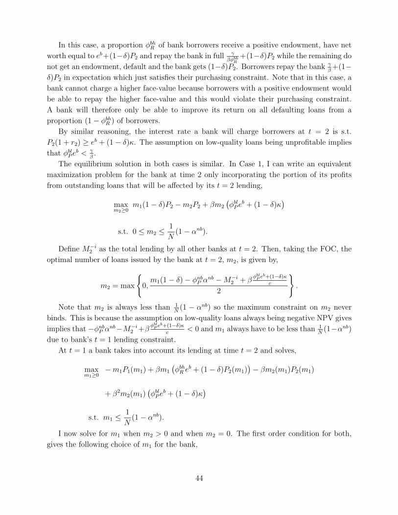
In this case, a proportion φbhR of bank borrowers receive a positive endowment, have net

worth equal to eb+(1−δ)P2 and repay the bank in full γβφbhR

+(1−δ)P2 while the remaining do

not get an endowment, default and the bank gets (1−δ)P2. Borrowers repay the bank γβ

+(1−δ)P2 in expectation which just satisfies their purchasing constraint. Note that in this case, a

bank cannot charge a higher face-value because borrowers with a positive endowment would

be able to repay the higher face-value and this would violate their purchasing constraint.

A bank will therefore only be able to improve its return on all defaulting loans from a

proportion (1− φbhR ) of borrowers.

By similar reasoning, the interest rate a bank will charge borrowers at t = 2 is s.t.

P2(1 + r2) ≥ eb + (1− δ)κ. The assumption on low-quality loans being unprofitable implies

that φblP eb < γ

β.

The equilibrium solution in both cases is similar. In Case 1, I can write an equivalent

maximization problem for the bank at time 2 only incorporating the portion of its profits

from outstanding loans that will be affected by its t = 2 lending,

maxm2≥0

m1(1− δ)P2 −m2P2 + βm2

(φblP e

b + (1− δ)κ)

s.t. 0 ≤ m2 ≤1

N(1− αnb).

Define M−i2 as the total lending by all other banks at t = 2. Then, taking the FOC, the

optimal number of loans issued by the bank at t = 2, m2, is given by,

m2 = max

{0,m1(1− δ)− φnbP αnb −M−i

2 + βφblP e

b+(1−δ)κc

2

}.

Note that m2 is always less than 1N

(1 − αnb) so the maximum constraint on m2 never

binds. This is because the assumption on low-quality loans always being negative NPV gives

implies that −φnbP αnb−M−i2 +β

φblP eb+(1−δ)κc

< 0 and m1 always have to be less than 1N

(1−αnb)due to bank’s t = 1 lending constraint.

At t = 1 a bank takes into account its lending at time t = 2 and solves,

maxm1≥0

−m1P1(m1) + βm1

(φbhR e

b + (1− δ)P2(m1))− βm2(m1)P2(m1)

+ β2m2(m1)(φblP e

b + (1− δ)κ)

s.t. m1 ≤1

N(1− αnb).

I now solve for m1 when m2 > 0 and when m2 = 0. The first order condition for both,

gives the following choice of m1 for the bank,

44

m1 = max

{0,min

{βc

(φbhR e

b + (1− δ)c(φnbP αnb +M−i2 +m2)

)− φnbR αnb −M−i

1

2,1− αnb

N

}}.

Note that the above solution is under the assumption that at t = 2, other banks take

m2 as given. This approach assumes that deviations at t = 1 from equilibrium are not

observable. An alternative approach involved other banks taking m2 as a function of m1 at

t = 2, in which case at t = 1 when a bank chooses m1, it would also take into account its

decision on M−i2 . The model solution if equilibrium deviations are observable is similar but

less tractable.

In Case 2, I can similarly write an equivalent maximization problem for the bank at time

2 only incorporating the portion of its profits from outstanding loans that will be affected

by its t = 2 lending,

maxm2≥0

(1− φbhR )m1(1− δ)P2 −m2P2 + βm2

(φblP e

b + (1− δ)κ)

s.t. 0 ≤ m2 ≤1

N(1− αnb).

Taking the FOC, the optimal number of loans issued by the bank at t = 2, m2, is given

by,

m2 = max

{0,

(1− φbhR )m1(1− δ)− φnbP αnb −M−i2 + β

φblP eb+(1−δ)κc

2

}.

The constraint m2 ≤ 1N

(1−αnb) will not bind for the same reason as in Case 1. At t = 1

a bank takes into account its lending at time t = 2 and solves,

maxm1≥0

−m1P1(m1) + βm1

(γ

β+ (1− δ)P2(m1)

)− βm2(m1)P2(m1)

+ β2m2(m1)(φblP e

b + (1− δ)κ)

s.t. m1 ≤1

N(1− αnb).

Taking the first order condition, the bank’s choice of m1 when m2 > 0 is given by,

m1 = max

0,min

βc

(γβ

+ (1− δ)c(φnbP αnb +M−i2 +m2)

)− φnbR αnb −M−i

1

2− β2(1− φbhR )φbhR (1− δ)2

,1− αnb

N

.

45

When m2 = 0, the bank’s choice of m1 is given by,

m1 = max

0,min

βc

(γβ

+ (1− δ)c(φnbP αnb +M−i2 +m2)

)− φnbR αnb −M−i

1

2,1− αnb

N

.

With commitment, the solution is similar. If φbhR eb ≤ γ

β, at t = 1 a bank will charge

borrowers,

P1(1 + r1) ≥ eb + (1− δ)P2.

The bank can set the interest rate equal to eb + (1− δ)P2. The bank now solves for both

m1 and m2 at t = 1. It therefore solves,

maxm1,m2≥0

−m1P1(m1) + βm1

(φbhR e

b + (1− δ)P2(m2))− βm2P2(m2)

+ β2m2

(φblP e

b + (1− δ)κ)

s.t. m1,m2 ≤1

N(1− αnb).

The first order conditions give,

m1 = max

{0,min

{βc

(φbhR e

b + (1− δ)c(φnbP αnb +M−i2 +m2)

)− φnbR αnb −M−i

1

2,1− αnb

N

}}.

m2 = max

{0,m1(1− δ)− φnbP αnb −M−i

2 + βφblP e

b+(1−δ)κc

2

}.

If φbhR eb > γ

β, at t = 1 a bank will charge borrowers,

P1(1 + r1) =γ

βφbhR+ (1− δ)P2.

The bank now solves for both m1 and m2 at t = 1. It therefore solves,

maxm1,m2≥0

−m1P1(m1) + βm1

(γ

β+ (1− δ)P2(m2)

)− βm2P2(m2)

+ β2m2

(φblP e

b + (1− δ)κ)

s.t. m1,m2 ≤1

N(1− αnb).

46

The first order conditions give,

m1 = max

0,min

βc

(γβ

+ (1− δ)c(φnbP αnb +M−i2 +m2)

)− φnbR αnb −M−i

1

2,1− αnb

N

.

m2 = max

{0,m1(1− δ)− φnbP αnb −M−i

2 + βφblP e

b+(1−δ)κc

2

}.

Proof of Proposition 1. I start the proof by showing that an equilibrium in symmetric

strategies exists and then show that this equilibrium is unique. I work through Case 1

in which the bank can not commit to future lending. Case 2 and the equilibrium with

commitment can be proved similarly.

I first consider equilibria in which all banks are propping up prices (m2 > 0), and then

equilibria in which no bank is propping up prices. I later show that these are the only two

possible equilibria, as an equilibrium in which some banks prop up prices and some do not,

does not exist.

First, I consider equilibria in which all banks prop up house prices (m2 > 0). Then, using

Lemma 1, at t = 2, a bank’s choice of m2 and m1 are given by,

m2 =m1(1− δ)− φnbP αnb −M−i

2 + βφblP e

b+(1−δ)κc

2.

m1 = min

{βc

(φbhR e

b + (1− δ)c(φnbP αnb +M−i2 +m2)

)− φnbR αnb −M−i

1

2,1− αnb

N

}.

If m1 = 0, m2 can never be greater than 0, therefore we can drop the minimum constraint

from m1.

In a symmetric equilibrium, M−i2 = (N − 1)m2 and M−i

1 = (N − 1)m1. Substituting

these into the above expressions, m1 and m2 are given by,

m2 =m1(1− δ)− φnbP αnb + β

φblP eb+(1−δ)κc

N + 1.

47

m1 = min

1

N + 1− β(1− δ)2 N(N+1)

β 1− δ2

φnbP αnb +(N − 1)

(−φnbP αnb + β

φblP eb+(1−δ)κc

)N + 1

+β2 1− δ

2c(φblP e

b + (1− δ)κ) +β

cφbhR e

b − φnbR αnb),1− αnb

N

}.

For N ≥ 1 The denominator of the RHS is increasing in N , while the numerator is

decreasing in N since by assumption −φnbP αnb+βφblP e

b+(1−δ)κc

< 0. Therefore m1 is decreasing

in N .

This is an equilibrium as long as banks want to make m2 > 0 at t = 2. This is the case

when,

m1(1− δ)− φnbP αnb + βφblP e

b + (1− δ)κc

> 0.

Rearranging,

m1 >φnbP α

nb − β φblP e

b+(1−δ)κc

1− δ.

Define N as the value of N at which m1 =φnbP αnb−β φ

blP eb+(1−δ)κc

1−δ . This is given by,

φnbP αnb − β φ

blP e

b+(1−δ)κc

1− δ= min

{βc

(φbhR e

b + (1− δ)cφnbP αnb)− φnbR αnb

N + 1,1− αnb

N

}.

This can be rearranged to give the following expression for N ,

N = min

{βc

((1− δ)φbhR eb + (1− δ)2cφnbP α

nb + φblP eb + (1− δ)κ

)− αnb((1− δ)φnbR + φnbP )

φnbP αnb − β φ

blP e

b+(1−δ)κc

,

(1− αnb)(1− δ)φnbP α

nb − β φblP e

b+(1−δ)κc

}.

Since m1 is decreasing in N , when N < N , an equilibrium in symmetric strategies in

which banks prop up prices exists.

Uniqueness: I now show that when all banks are propping up prices, the symmetric

equilibrium is the unique equilibrium. We can write any given bank’s t = 1 and t = 2

48

optimal lending in terms of prices,

m2 = m1(1− δ)− P2

c+β

c

(φblP e

b + (1− δ)κ).

m1 = min

{β

cφblP e

b +β

c(1− δ)P2 −

P1

c,1− αnb

N

}.

Since all banks face the same P1 and P2, if this equilibrium exists, all players must be

behaving symmetrically. When banks are behaving symmetrically the equilibrium solution

is unique (calculated above). Therefore, the symmetric equilibrium is the unique equilibrium

when banks are propping up house prices.

I now consider equilibria in which banks do not prop up house prices. Similar to the case

before, I first establish an equilibrium in symmetric strategies is which banks do not prop

up prices and then show that this is the unique equilibrium.

When the bank is not propping up prices, m2 = 0. In this case P2 = cαnbφnbP . At t = 1,

a bank solves,

maxm1 −m1P1(m1) + βm1(φbhR eb + (1− δ)cαnbφnbP ).

The FOC is given by,

− cm1 − c(αnbφnbR +m1 +M−i1 ) + βφbhR e

b + β(1− δ)cαnbφnbP = 0.

m1 = max

{0,min

{βφbhR e

b

c+ β(1− δ)αnbφnbP − αnbφnbR −M−i

1

2,1− αnb

N

}}.

In a symmetric equilibrium,

m1 = max

{0,min

{βφbhR e

b

c+ β(1− δ)αnbφnbP − αnbφnbR

N + 1,1− αnb

N

}}.

This is an equilibrium as long as banks do not want to make m2 > 0 at t = 2. This is

the case when,

m1(1− δ)− φnbP αnb + βφblP e

b + (1− δ)κc

≤ 0.

This is satisfied whenever N ≥ N .

Uniqueness: Uniqueness follows as it did before when banks are not propping up prices.

We can write any given bank’s t = 1 and t = 2 optimal lending in terms of prices,

m2 = 0.

49

m1 = max

{0,min

{β

cφblP e

b +β

c(1− δ)P2 −

P1

c,1− αnb

N

}}.

Since all banks face the same P1 and P2, if this equilibrium exists, all players must be

behaving symmetrically. When banks are behaving symmetrically the equilibrium solution

is unique (calculated above). Therefore, the symmetric equilibrium is the unique equilibrium

when banks are propping up house prices.

To complete the proof, I also need to rule out the case when some banks are propping

up prices and some are not. I prove this by contradiction. Imagine bank i is propping up

prices and bank j is not. Then at t = 1,

mi1 = min

{β

cφblP e

b +β

c(1− δ)P2 −

P1

c,1− αnb

N

}.

mj1 = max

{0,min

{β

cφblP e

b +β

c(1− δ)P2 −

P1

c,1− αnb

N

}}.

These expressions imply that mi1 = mj

1. However,if this is the case, mj2 = mi

1 which is a

contradiction. Therefore, in any equilibrium either all banks will be propping up prices, or

no bank will be propping up prices.

For Case 2 without commitment, the proposition can be proven in a similar way. In this

case, N is given by the following expression,

N = min

{βc

((1− δ)(1− φbhR )φbhR e

b + (1− δ)2(1− φbhR )cφnbP αnb + φblP e

b + (1− δ)κ)

φnbP αnb − β φ

blP e

b+(1−δ)κc

−αnb((1− δ)(1− φbhR )φnbR + φnbP )

φnbP αnb − β φ

blP e

b+(1−δ)κc

,(1− αnb)(1− φbhR )(1− δ)φnbP α

nb − β φblP e

b+(1−δ)κc

}.

With commitment, N is given by,

N = min

βc

((1− δ) min

{φbhR e

b, γβ

}+ (1− δ)2cφnbP α

nb + φblP eb + (1− δ)κ

)− αnb((1− δ)φnbR + φnbP )

φnbP αnb − β φ

blP e

b+(1−δ)κc

,

(1− αnb)(1− δ)φnbP α

nb − β φblP e

b+(1−δ)κc

}.

50

Proof of Corollary 1. Consider Case 1 without commitment. If N ≥ N , banks do

not prop up prices in equilibrium. The total credit extended at t = 1 by a single bank is

given by,

m1 = max

{0,min

{βφbhR e

b

c+ β(1− δ)αnbφnbP − αnbφnbR

N + 1,(1− α)nb

N

}}.

When N ≥ N , as N increases, m1 decreases. m2 = 0 for all N ≥ N . Therefore when

N ≥ N , credit by any given bank increases as N decreases.

Total credit at t = 2 is M2 = 0. Total credit at t = 1 is given by,

M1 = max

{0,min

{NβφbhR e

b

c+ β(1− δ)αnbφnbP − αnbφnbR

N + 1, (1− α)nb

}}.

This is increasing in N .

If N < N , the economy is in an equilibrium in which banks prop up house prices. The

total credit at t = 1 extended by a single bank is given by,

m1 =1

N + 1− β (1−δ)22− β(1− δ)2 N−1

2(N+1)

β 1− δ2

φnbP αnb +(N − 1)

(−φnbP αnb + β

φblP eb+(1−δ)κc

)N + 1

+β2 1− δ

2c(φblP e

b + (1− δ)κ) +β

cφbhR e

b − φnbR αnb).

m1 increases as N decreases (from the proof of Proposition 1). The total credit at t = 2

extended by a single bank is given by,

m2 =m1(N)(1− δ)− φnbP αnb + β

φblP eb+(1−δ)κc

N + 1.

As N decreases, m2 increases. Therefore, the total credit extended by a single bank

increases as N decreases.

The total credit in the economy is given by,

51

M1 +M2 =N

N + 1− β (1−δ)22− β(1− δ)2 N−1

2(N+1)

(1 +

1− δN + 1

)(β

1− δ2

(φnbP α

nb+

(N − 1)(−φnbP αnb + β

φblP eb+(1−δ)κc

)N + 1

+ β2 1− δ2c

(φblP eb + (1− δ)κ+ φbhR e

b

−φnbR αnb))

+N

N + 1

(−φnbP αnb + β

φblP eb + (1− δ)κ

c

).

Taking the derivative w.r.t N ,

− ((1− δ)2β + (1− δ)− 1)N2 − 2N − (1− δ)− 1

(N2 + (2− (1− δ)2β)N + 1)2

(β

1− δ2

φnbP αnb + β2 1− δ

2c(φblP e

b + (1− δ)κ)

+β

cφbhR e

b − φnbR αnb)−

−φnbP αnb + βφblP e

b+(1−δ)κc

(N + 1)2 (N2 + (2− (1− δ)2β)N + 1)2

(((1− δ)2β + 1− δ − 4

)N4

+(4(1− δ)2β − 2(1− δ)− 12

)N3 +

(−(1− δ)4β2 +

(2(1− δ)3 + 5(1− δ)2

)β − 6(1− δ)− 12

)N2

+2((1− δ)2β − 2(1− δ)− 4)N + 1− δ).

The second term in the above expression is always negative and this can cause the value of

the total derivative to be negative.35 Therefore aggregate credit can increase as N decreases.

The proof in Case 2 and the case with commitment follow similarly.

Proof of Corollary 2. Consider Case 1 without commitment. From Proposition 1, N

is given by,

N = min

{βc

((1− δ)φbhR eb + (1− δ)2cφnbP α

nb + φblP eb + (1− δ)κ

)− αnb((1− δ)φnbR + φnbP )

φnbP αnb − β φ

blP e

b+(1−δ)κc

,

(1− αnb)(1− δ)φnbP α

nb − β φblP e

b+(1−δ)κc

}.

35For N ≥ 1, the multiplier on φnbP αnb and φnbR α

nb are always negative. The mathematics of when exactlythis expression is negative is tedious and does not add anything much to understanding the main mechanismin the paper but can be made available on request. An example of this can be seen in the graphical illustrationin the paper.

52

It is straightforward from the above expression that,

∂N

∂(φblP eb)> 0.

As δ increases, the denominator in the expression for N increases. At the same time the

numerator of the above expression is decreasing. To see this clearly for the first term of the

minimization, taking the derivative of the numerator of N w.r.t. δ, we get,

− β

c

(φbhR e

b + 2(1− δ)cφnbP αnb + κ)

+ αnbφnbR (1)

Recall from Proposition 1, that when banks are not propping up prices,

m1 = max

{0,min

{βφbhR e

b

c+ β(1− δ)αnbφnbP − αnbφnbR

N + 1,1− αnb

N

}}.

Therefore, in the relevant range, βcφbhR e

b + β(1 − δ)φnbP αnb − αnbφnbR > 0 since m1 ≥ 0.

This implies that (3) is negative. Therefore N is decreasing in δ.

Similarly as φnbP increases, the denominator of N is increasing. Additionally in the first

term of the minimization, the numerator is decreasing: taking the derivative of the numerator

of N w.r.t. φnbP , we get,

αnb(β(1− δ)2 − 1) < 0.

Therefore N is decreasing in φnbP .

The proof in Case 2 and the case with commitment follow similarly.

Proof of Proposition 2. For any default costs, d > 0, the total welfare under N1 is

(M1(N1) +M2(N1) + (φnbP + φnbR )αnb)γ + βeb(φbhR + φbhP )(1− αnb) + 2βαnbenb

− βd(M1(N1)(1− φbR)M2(N1)(1− φbP ))

The total welfare under N2 is

(M1(N2) + (φnbP + φnbR )αnb)γ + βeb(φbhR + φbhP )(1− αnb) + 2βαnbenb

− βd(M1(N1)(1− φbR))

Since M1(N2) = M1(N1) + M2(N1), φbR > φbP and d > 0, welfare is always higher under

N2 than N1.

Proof of Proposition 3. Consider Case 1. Since N depends on φblP and φnbP , this

53

proposition only compares areas given an N1 and N2 s.t. N for each area falls within

(N1, N2]. Following an increase in concentration from N1 ≥ N to N2 < N , the change in

total lending is given by,

∆M =

(N2 +

(1− δ)N2

N2 + 1

) β 1−δ2

φnbP αnb +(N2−1)

(−φnbP αnb+β

φblP eb+(1−δ)κc

)N2+1

+ β2(1−δ)2c

(φblP eb + (1− δ)κ)

N2 + 1− β (1−δ)22− β(1− δ)2 N2−1

2(N2+1)

+N2

(1 +

1− δN2 + 1

) βcφbhR e

b − φnbR αnb

N2 + 1− β (1−δ)22− β(1− δ)2 N2−1

2(N2+1)

+N2

N2 + 1

(−φnbP αnb + β

φblP eb + (1− δ)κ

c

)−N1

βφbhR e

b

c+ β(1− δ)αnbφnbP − αnbφnbR

N1 + 1.

(2)

Taking the derivative w.r.t φnbP ,

∂∆M

∂φnbP= N2

(1 +

1− δN2 + 1

) β 1−δ2

(αnb − (N2−1)αnb

N2+1

)N2 + 1− β(1− δ)2 N2

N2+1

− N2αnb

N2 + 1−N1β

(1− δ)αnb

N1 + 1.

If ∂∆M∂φnbP

< 0, then income growth and the growth in mortgage credit can be negatively

correlated. For this to be the case, we require that,

N2

(1 +

1− δN2 + 1

)β(1− δ) αnb

N2+1

N2 + 1− β(1− δ)2 N2

N2+1

− N2αnb

N2 + 1−N1β

(1− δ)αnb

N1 + 1< 0.

Simplifying,

(1− δ) N2 + 2− δN2

2 + 1 + 2N2 − β(1− δ)2N2

N2

N2 + 1− 1

β

N2

N2 + 1−N1

1− δN1 + 1

< 0.

The denominator of the coefficient multiplying the first term is greater than the numerator.

Therefore the first term is strictly less that the value of the second term and this expression

is always less than 0. Therefore, ∂∆M∂φnbP

< 0.

Looking at (2), we can see that all the terms multiplying φblP are always positive. Therefore,∂∆M∂φblP

> 0.

The proof in Case 2 and the case with commitment follow similarly.

54

Proof of Proposition 4. I start the proof by simplifying the problem in a similar

way to the three-period model by focusing on the bank’s choice of interest rate. Given state-

contingent repayments, state by state, a bank will charge the maximum interest rate such

that borrowers are willing to pay. Consider the interest rate a bank will charge borrowers

from generation t when the state of the world is st ∈ {R,P}. As in the three-period model,

depending on the relative values of φbhst , φblst and γ, there are various possible cases. Here, I will

work through the interest rate problem in the case in which φbhR eb < γ

βwithout commitment.

The other cases are similar.

If φbjsteb < γ

β, where j = {h, l} represents borrower-type, a bank will charge:

Pt−1(1 + rt−1(st)) > eb + (1− δ)Pt(st).

In this case, a proportion φbjst of bank borrowers get a positive endowment and pay the

bank eb + (1− δ)Pt(st) while the remaining do not get an endowment and pay the bank gets

(1−δ)Pt(st). In expectation, borrowers repay the bank φbjsteb+(1−δ)E[Pt(st)] which satisfies

their purchasing constraint. When φbhR eb < γ

β, because of the assumptions on the income of

high- versus low-quality borrowers and in rich versus poor states, φbjsteb < γ

β, ∀st, ∀j. As in

the three-period case, in the model without commitment, banks can only credibly prop up

house prices to improve their return on loans when the borrower cannot repay the full face-

value of the loan. State-by-state the bank will therefore choose a facevalue that is strictly

higher than eb + (1− δ)Pt(st).In this case, define mt = mh

t +mlt. Then, we can write the bank’s maximization problem

at any time t as:

V (st,mt−1) = maxmht ≥0,mlt≥0

mt−1(1− δ)Pt −∑

j={h,l}

mjtPt + β

∑j={h,l}

mjtφ

bjste

b + βE [V (st+1,mt)]

s.t. mht ≤

1

Nαbh, s.t. ml

t ≤1

N(1− αbh − αnb).

The above problem is independent of interest rates chosen by the bank. Therefore each

period a bank only decides on the amount of loans they wish to issue to each type of borrower.

Further, it is independent of the income of generation t− 1. The housing price only depends

on the total number of loans outstanding to generation t − 1. In this case, the problem is

also independent of the type of loans made to high- versus low-quality borrowers at t − 1

but in other cases, it is not.

Using the envelope theorem,

∂E [V (st+1,mt)]

∂mht

=∂E [V (st+1,mt)]

∂mlt

= (1− δ)E[Pt+1]

55

This gives the following FOCs for a bank,

∂V (st,mt−1)

∂mht

= mt−1(1− δ)c− Pt −mht c+ βφbhst e

b + β(1− δ)E[Pt+1].

∂V (st,mt−1)

∂mlt

= mt−1(1− δ)c− Pt −mltc+ βφblste

b + β(1− δ)E[Pt+1].

The equilibrium lending by a bank is given by,

mht = max

{0,min

{mt−1(1− δ)c− Pt + βφbhst e

b + β(1− δ)E[Pt+1]

c,αbh

N

}}.

mlt = max

{0,min

{mt−1(1− δ)c− Pt + βφblste

b + β(1− δ)E[Pt+1]

c,1− αbh − αnb

N

}}.

Given a choice of lending to high-quality borrowers over low-quality borrowers, it is always

dominant for a bank to make a loan to a high-quality borrower. Therefore, if,

mt−1(1− δ)c− Pt + βφbhst eb + β(1− δ)E[Pt+1]

c≤ αbh

N

mlt = 0.

I now show an equilibrium is always symmetric if all banks start with the same level of

initial loans m0. Consider a bank’s lending at t = 1.

mh1 = max

{0,min

{m0(1− δ)c− P1 + βφbhst e

b + β(1− δ)E[P2]

c,αbh

N

}}.

ml1 = max

{0,min

{m0(1− δ)c− P1 + βφblste

b + β(1− δ)E[P2]

c,1− αbh − αnb

N

}}.

If all banks have the same m0, then the above equations will be identical for all banks

and they will choose the same m1. Similarly at t = 2, we can show that if all banks have

the same m1, they will choose the same m2 and so on and so forth. Given the symmetric

equilibrium solution, I can rewrite equilibrium lending as,

56

Mht

N= max

{0,min

{Mt−1

N(1− δ)c− cMh

t − cM lt − cαnbφnbst + βφbhst e

b + β(1− δ)E[Pt+1]

c,αbh

N

}}.

(3)

M lt

N= max

{0,min

{Mt−1

N(1− δ)c− cMh

t − cM lt − cαnb + βφbhst e

b + β(1− δ)E[Pt+1]

c,1− αbh − αnb

N

}}.

(4)

Given these first order conditions, I can write an equivalent maximization problem of a

representative bank in this economy. This is given by,

V (st,Mt−1) = maxMht ≥0,M l

t≥0

Mt−1

N(1− δ)Pt +

∑j={h,l}

(−M

jt

NPt −

N − 1

N

M jt

2

2c− (N − 1)

NM j

t φnbst α

nbc+ βM jt φ

bjste

b

)

− (N − 1)

NMh

t Mltc+ βE [V (st+1,Mt)]

s.t. Mht ≤ αh

s.t. M lt ≤ 1− αh − αnb.

The first order conditions for this representative bank give the same aggregate lending

as those of the individual banks. I can show that the above maximization of the equivalent

representative bank is a contraction mapping. Define

U(st,Mt−1,Mht ,M

lt) =

Mt−1

N(1− δ)Pt+

∑j={h,l}

(−M

jt

NPt −

N − 1

N

M jt

2

2c− (N − 1)

NM j

t φnbst α

nbc+ βM jt φ

bjste

b

)− (N − 1)

NMh

t Mltc

Since Mht , M l

t and Mt−1 are bounded, Pt is bounded and therefore U is bounded. Define

an operator,

57

(TV )(st,Mt−1) = max0≤Mh

t ≤αbh, 0≤M lt≤1−αbh−αnb

{U(st,Mt−1,M

ht ,M

lt) + βE [V (st+1,Mt)]

}.

Take V to be bounded. Since U is bounded by assumption, then TV is also bounded.

TV satisfies monotonicity. Suppose V < W . Let gh(Mt−1, st) and gl(Mt−1, st) be the optimal

policy functions (not necessarily unique) corresponding to V for Mht and M l

t respectively.

Then for all Mt−1 ∈ [0, 1− αnb],

TV (st,Mt−1) = U(st,Mt−1, gh(Mt−1, st), gl(Mt−1, st)) + βE [V (st+1 + gh(Mt−1, st), gl(Mt−1, st))]

≤ U(st,Mt−1, gh(Mt−1, st), gl(Mt−1, st)) + βE [W (st+1, gh(Mt−1, st) + gh(Mt−1, st))]

≤ max0≤Mh

t ≤αbh, 0≤M lt≤1−αbh−αnb

{U(st,Mt−1,M

ht ,M

lt) + βE

[W (st+1,M

ht +M l

t))]}

= TW (st,Mt−1)

.

TV also satisfies discounting. Let a > 0. Then,

T (V + a)(st,Mt−1) = max0≤Mh

t ≤αbh, 0≤M lt≤1−αbh−αnb

{U(st,Mt−1,M

ht ,M

lt) + βE [V (st+1,Mt) + a]

}= max

0≤Mht ≤αbh, 0≤M l

t≤1−αbh−αnb

{U(st,Mt−1,M

ht ,M

lt) + βE [V (st+1,Mt)]

}+ βa

= TV (st,Mt−1) + βa

.

The model therefore satisfies Blackwell’s conditions and is bounded and is therefore a

contraction mapping with modulus β. Therefore, an equilibrium of this economy exists and

can be found through value function iteration.

The Hessian matrix of U is given by,(−N+1

Nc − N−1

Nc

−N−1Nc − N+1

Nc

).

The determinant of the Hessian is given by,(N + 1

Nc

)2

−(N − 1

Nc

)2

< 0.

The Hessian matrix is negative semi-definite since the determinant is less than 0 and

58

−N+1Nc < 0. Therefore, for all Mh

t and M lt , U is a strictly concave function. Let SMt be the

set of all possible values of Mt. Then since SMt is convex, the correspondence which gives

the set of all feasible allocations given Mt is convex, and U is continuous and bounded, there

is a unique policy function associated with the above problem and V ∗ is strictly concave.

The equilibrium is therefore unique.

From (3) and (4), it is straightforward that conditional on the state of the economy, Mt

is linearly increasing in Mt−1. Furthermore, due to linearity, conditional on state, Mht is

strictly increasing in Mht−1 when Mh

t−1 < αbh.

An equilibrium in which banks do not make any loans to low-quality borrowers to prop-up

prices is equivalent to an equilibrium in which ∀t and ∀s,(Mt−1

N(1− δ)c− cMh

t − cαnb + βφbhst + β(1− δ)E[Pt+1]

)N

c(N + 1)≤ 0

Since Mt is linearly increasing in Mt−1 (and strictly increasing in the range Mt−1 ∈[0, αbh

), then ∃ T s.t. a series of T consecutive R shocks that will eventually give MT = αbh

(as long as V (R,M0) > 0). Since the incentive to prop up prices is highest when outstanding

loans are the highest, if at T + 1, in either state, a bank does not want to prop up prices

given that they expect no other banks to be propping up prices, then for any series of shocks

banks make no loans to low-quality borrowers. Substituting in Mt−1 = αbh into the above

condition, such an equilibrium exists when,(αbh

N(1− δ)c− cMh

t − cαnb + βφbhst + β(1− δ)E[Pt+1]

)N

c(N + 1)≤ 0

Since banks will always make high-quality loans before low-quality loans, this implies

that Mht = αbh. Substituting this in,

αbh

N(1− δ)c− cαbh − cαnb + βφbhst + β(1− δ)E[Pt+1] ≤ 0

The LHS is decreasing asN increases. Note that Pt+1(Mt−1, st) is increasing in outstanding

loans per bank, Mt−1

N, and therefore as N increases, E[Pt+1] decreases. Therefore, ∃N s.t.

when N ≥ N , an equilibrium in which banks do not prop up house prices exists. When

N < N , bank will make loans to low-quality borrowers and prop up prices. The other cases

can be worked through similarly.

Proof of Corollary 3.

The proof for this is contained in in the proof for Proposition 3. Please refer to that

above.

59

Appendix B

Income Growth and Mortgage Growth with Borrower Heterogeneity

In the three-period model in the main text it is clear that non-borrower income growth can

cause there to be a negative correlation between credit and income-growth when looking at

an area following an increase in concentration. However, to additionally be able to show that

a positive correlation can still exist between credit and income growth at the borrower-level,

we need to allow for borrower level heterogeneity. To illustrate the two results simultaneously,

it is enough to allow borrower-level heterogeneity at t = 2 and look at t = 2 credit when

concentration changes. At t = 2, let there be a proportion αbh of high-quality borrowers

who get an endowment with probability φbhR . Then we get the following graphs for credit at

a borrower-level versus an area-level as concentration changes.

Figure 8: The figure on the left plots total credit, measured by the number of households who get amortgage, against the level of concentration in the mortgage market for different income growths betweent = 1 and t = 2. The figure on the right plots credit received by high-quality borrowers versus by low-qualityborrowers inside the area with lower-income growth against the level of concentration. As we move alongthe x-axis, N increases and concentration decreases. The parametrization is as follows: δ = .01, αnb = .2,φblP = .2, φbhR = 1, φnbR = 1, eb = 2 ,κ = .45, γ = 4, b = 9.8, αbh = .01, φbhP = .41 . φnbP is varied to getchanges in income growth across the two plots - it is equal to .73 is the high-income growth area and .7 inthe low-income growth area.

60

Appendix C

Calibration of Main Model

Data Description: The fraction of sub-prime borrowers is from a research report by the

Financial Inquiry Commission using data from Inside Mortgage Finance. U.S. house price

changes are calculated from Federal Reserve Economic Data. The home-ownership rate is

taken from the U.S. Census Bureau. The default rates on prime and sub-prime loans are

taken from a research report by the U.S. Census Bureau. The fraction of cash-only house

purchases are from RealtyTrac. The private benefit of home-ownership is hard to measure

in the data and therefore I choose a value of γ so that it does not determine any equilibrium

quantities.

Table 1: Configuration of Model Parameters

Description Symbol Value Source/Target

Fraction of high-quality borrowers αbh .5 Loans to prime borrowers

Fraction of non-borrowers αnb .06 Cash only house purchases

Low-quality borrower shock rich state φblR .9 Default rate on sub-prime loans in boom

Low-quality borrower shock poor state φblP .75 Default rate on sub-prime loans in bust

High-quality borrower shock rich state φbhR .98 Default rate on prime loans in boom

High-quality borrower shock poor state φbhP .94 Default rate on prime loans in bust

Discount Factor β .99 Standard

Depreciation δ .02 Standard

Number of banks N 2 Mortgage market concentration

Borrower endowment eb 2.4 House prices, sub-prime fraction

Construction cost c 5.6 House prices, sub-prime fraction

Likelihood of rich state q .5 House prices, sub-prime fraction

To limit the number of free parameters, γ ≥ 2.6, φnbR = φnbP = 1.

Table 2: Aggregate Moments

Model Data

Fraction of sub-prime borrowers in boom .12 .12

Fraction of sub-prime borrowers in bust .05 .05

Default rate sub-prime loans in boom .10 .12

Default rate sub-prime loans in bust .25 .25

Default rate prime loans in boom .02 .02

Default rate on prime loans in bust .06 .06

Fraction of cash only house purchases boom .09 .13

Fraction of cash only house purchases bust .10 .22

House price increase boom .52 1.43

House price decrease bust -.11 -.20

Change home-ownership rate boom .07 .05

Change home-ownership rate bust .07 .02

In the model without commitment, since the banks charge a face-value slightly higher than eb + (1− δ)P2,

I consider a mortgage as delinquent when borrowers repay the banks less than eb + (1− δ)P2.

Table 3: Counter factual Analysis

N=2 N=4

Fraction of sub-prime borrowers in boom .12 0

Fraction of sub-prime borrowers in bust .05 0

House price increase boom .52 .22

House price decrease bust -.23 -.03

Calibration of Model with Dispersed Lenders

Data Description: The data is as before. The GSE market share is calculated from the

Federal Reserve and Federal Housing Finance.

Table 4: Configuration of Model Parameters

Description Symbol Value Source/Target

Fraction of high-quality borrowers αh .5 Fraction of prime/sub-prime borrowers

Fraction of non-borrowers αnb .06 Fraction of cash only house purchases

Low-quality borrower shock rich state φblR .9 Default rate on sub-prime loans in boom

Low-quality borrower shock poor state φblP .75 Default rate on sub-prime loans in bust

High-quality borrower shock rich state φbhR .98 Default rate on prime loans in boom

Low-quality borrower shock poor state φbhP .95 Default rate on prime loans in bust

Discount Factor β .99 Standard

Depreciation δ .02 Standard

borrower endowment eb 1.4 house price boom/bust

Elasticity c 5.8 house price boom/bust

Number of banks N 2 Mortgage market concentration

Borrower share of dispersed banks s .6 Mortgage market concentration

Likelihood of rich state q .5

To limit the number of free parameters, γ ≥ 1.4, φnbR = φnbP = 1.

Table 5: Aggregate Moments

Model Data

Fraction of sub-prime borrowers in boom .11 .12

Fraction of sub-prime borrowers in bust .07 .05

Default rate sub-prime loans in boom .10 .12

Default rate sub-prime loans in bust .25 .25

Default rate prime loans in boom .02 .02

Default rate on prime loans in bust .06 .06

Fraction of cash only house purchases boom .18 .13

Fraction of cash only house purchases bust .20 .22

House price increase boom .63 1.43

House price decrease bust -.06 -.20

Change home-ownership rate boom .08 .05

Change home-ownership rate bust .02 .02

GSE Market Share ’07 .42 .42

In the model without commitment, since the banks charge a face-value slightly higher than eb + (1− δ)P2,

I consider a mortgage as delinquent when borrowers repay the banks less than eb + (1− δ)P2.

Table 6: Counter factual Analysis

N=2 N=4

Fraction of sub-prime borrowers in boom .11 0

Fraction of sub-prime borrowers in bust .07 0

House price increase boom .63 .45

House price decrease bust -.06 -.01

Appendix D

GSE Share of Mortgage Debt in the United States

Figure 9: The above figure plots Fannie Mae and Freddie Mac’s share of the all outstanding US mortgagedebt. Source: Federal Reserve and Federal Housing Finance.

GSE Dollar Exposure of Mortgage Debt in the United States

Figure 10: The above figure plots Fannie Mae and Freddie Mac’s total dollar exposure to the US housingmarket. Source: Federal Reserve and Federal Housing Finance.