toda system and cluster phase transition layers in an ...jcwei/wy-asynal-r.pdftoda system and...
TRANSCRIPT
Toda system and cluster phase transition layers in an
inhomogeneous phase transition model
Juncheng Wei
Department of Mathematics, The Chinese University of Hong Kong,
Shatin, Hong Kong. Email: [email protected]
Jun Yang
College of Mathematics and Computational Sciences, Shenzhen University,
Nanhai Ave 3688, Shenzhen, China, 518060. Email: [email protected]
Abstract
We consider the following singularly perturbed elliptic problem
ε24u +(u− a(y)
)(1− u2) = 0 in Ω,
∂u
∂ν= 0 on ∂Ω,
where Ω is a bounded domain in R2 with smooth boundary, −1 < a(y) < 1, ε is a small
parameter, ν denotes the outward normal of ∂Ω. Assume that Γ = y ∈ Ω : a(y) = 0 is
a simple closed and smooth curve contained in Ω in such a way that Γ separates Ω into two
disjoint components Ω+ = y ∈ Ω : a(y) < 0 and Ω− = y ∈ Ω : a(y) > 0 and ∂a∂ν0
> 0 on
Γ, where ν0 is the outer normal of Ω+, pointing to the interior of Ω−. For any fixed integer
N = 2m+1 ≥ 3, we will show the existence of a clustered solution uε with N -transition layers
near Γ with mutual distance O(ε| log ε|), provided that ε stays away from a discrete set of
values at which resonance occurs. Moreover, uε approaches 1 in Ω− and −1 in Ω+. Central
to our analysis is the solvability of a Toda system.
1 Introduction
Let Ω be a bounded and smooth domain in R2. In gradient theory of phase transition it is common
to seek for critical points in H1(Ω) of an energy of the form
Jε(u) =ε
2
∫Ω
|∇u|2 +1ε
∫Ω
W (y, u) (1.1)
1

where W (y, ·) is a double-well potential with exactly two strict local minimizers at u = −1 and
u = +1, which as well correspond to trivial local minimizers of Jε in H1(Ω). For simplicity of
exposition we shall restrict ourselves to a potential of the form
W (y, u) =∫ u
−1
(s2 − 1)(s− a(y)
)ds, (1.2)
for a smooth function a(y) with
−1 < a(y) < 1 for all y ∈ Ω.
Critical points of Jε correspond to solutions of the problem
ε24u +(u− a(y)
)(1− u2) = 0 in Ω,
∂u
∂ν= 0 on ∂Ω, (1.3)
where ε is a small parameter, ν denotes the outward normal of ∂Ω. Function u represents a
continuous realization of the phase present in a material confined to the region Ω at the point x
which, except for a narrow region, is expected to take values close to +1 or −1. Of interest are of
course non-trivial steady state configurations in which the antiphases coexist.
The case a ≡ 0 corresponds to the standard Allen-Cahn equation [6]
ε24u + u(1− u2) = 0 in Ω,∂u
∂ν= 0 on ∂Ω, (1.4)
for which extensive literature on transition layer solution is available, see for instance [4, 9, 23, 27,
28, 31, 32, 33, 34, 35, 37, 38, 39, 40, 43], and the references therein for these and related issues.
In this paper, we consider the inhomogeneous Allen-Cahn equation, i.e, problem (1.3). Let us
assume that Γ = y ∈ Ω : a(y) = 0 is a simple, closed and smooth curve in Ω which separates
the domain into two disjoint components
Ω = Ω− ∪ Γ ∪ Ω+ (1.5)
such that
a(y) < 0 in Ω+, a(y) > 0 in Ω−,∂a
∂ν0> 0 on Γ, (1.6)
where ν0 is the outer normal of Ω+, pointing to the interior of Ω−. Observe in particular that for
the potential (1.2), we have
W (y,−1) < W (y, 1) in Ω−, W (y,+1) < W (y,−1) in Ω+.
Thus, if one consider a global minimizer uε for Jε, which exists by standard arguments, it should
be such that its value want to minimize W (y, u), namely, uε should intuitively achieve as ε→ 0,
uε → −1 in Ω− uε → +1 in Ω+. (1.7)
2
A solution uε to problem (1.3) with these properties was constructed, and precisely described,
by Fife and Greenlee[22] via matching asymptotic and bifurcation arguments. Super-subsolutions
were later used by Angenent, Mallet-Paret and Peletier in the one dimensional case (see [7]) for
construction and classification of stable solutions. Radial solutions were found variationally by
Alikakos and Simpson in [5]. These results were extended by del Pino in [12] for general (even non
smooth) interfaces in any dimension, and further constructions have been done recently by Dancer
and Yan [11] and Do Nascimento [18]. In particular, it was proved in [11] that solutions with the
asymptotic behavior like (1.7) are typically minimizer of Jε. Related results can be found in [1, 2].
On the other hand, a solution exhibiting a transition layer in the opposite direction, namely
uε → +1 in Ω− and uε → −1 in Ω+ as ε→ 0, (1.8)
has been believed to exist for many years. Hale and Sakamoto [25] established the existence of this
type of solution in the one-dimensional case, while this was done for the radial case in [13], see
also [10]. The layer with the asymptotics in (1.8) in this scalar problem is meaningful in describing
pattern-formation for reaction-diffusion systems such as Gierer-Meinhardt with saturation, see
[13, 21, 36, 41] and the references therein.
Recently this problem has been completely solved by del Pino-Kowalczyk-Wei [15] (in the two
dimensional domain case) and Mahmoudi-Malchiodi-Wei [30] (in the higher dimensional case).
More precisely, defining
λ∗ =1
3π2
∫RH2x dx
[∫Γ
öa
∂ν0
]2
, (1.9)
where H(x) is the unique heteroclinic solution of
H′′
+H −H3 = 0 in R, H(0) = 0, H(±∞) = ±1, (1.10)
in [15], M. del Pino, M. Kowalczyk and J. Wei proved the existence of a transition layer solution
Hε in the opposite direction, namely,
Theorem 1.1. Given c > 0, there exists ε0 > 0 such that for all ε < ε0 satisfying the gap condition∣∣∣j2ε− λ∗∣∣∣ ≥ c√ε for all j ∈ N, (1.11)
problem (1.3) has a solution Hε satisfying
Hε → +1 in Ω−, Hε → −1 in Ω+ as ε→ 0. (1.12)
Moreover, the layer will approach the curve Γ as ε→ 0.
3

We will extend Theorem 1.1 and prove the following main result for the existence of clustering
transition layers in this paper. Let ` = |Γ| denote the total length of Γ. We consider natural
parameterization γ(θ) of Γ with positive orientation, where θ denotes arclength parameter measured
from a fixed point of Γ. Points y, which are δ0−close Γ for sufficiently small δ0, can be represented
in the form
y = γ(θ) + t ν0(θ), |t| < δ0, θ ∈ [0, `), (1.13)
where the map y 7→ (t, θ) is a local diffeomorphism. By slight abuse of notation we denote a(t, θ)
to actually mean a(y) for y in (1.13). The main theorem reads
Theorem 1.2. For any fixed integer N = 2m + 1 ≥ 3, there exists a sequence (εl)l approaching
0+ such that problem (1.3) has a clustered solution uεl with N -phase transition layers with mutual
distance O(εl| log εl|). Moreover, uεl approaches 1 in Ω− and −1 in Ω+. Near Γ, uεl has the form
uεl ∼N∑n=1
H
(t− εlen(θ)
εl
),
where t is the sign distance to the curve Γ along the normal direction ν0 and θ denotes arclength
parameter measured from a fixed point of Γ. The functions en’s satisfy
‖en‖∞ ≤ C| log εl|2, min1≤n≤N−1
(en+1 − en) >√
22| log εl|.
More precisely,
en = (−1)n+1f + fn with f(θ) =k(θ)√
2 at(0, θ),
where k(θ) denotes the curvature of Γ. All functions fn, n = 1, . . . , N solve the Toda system, for
n = 1, . . . , N,
ε2l γ0f
′′n + εl (−1)n+1 α1(θ) fn − γ1
[e−(fn−fn−1+βn
)− e−
(fn+1−fn+βn+1
) ]= 0 in (0, `), (1.14)
f ′n(0) = f ′n(`), fn(0) = fn(`), (1.15)
for two universal constant γ0, γ1 > 0 and α1(θ) = 43at(0, θ) > 0, with the conventions βn =
2(−1)nf, f0 = −∞, fN+1 =∞.
Remark 1: In [11], under the condition that a = a(r), a(r0) = 0, a′(r0) 6= 0, Dancer and Yan
showed the existence of solutions with N = 2m+ 1 interfaces, provided that ε is small. Therefore
they proved Theorem 1.2 in the radial case. Due to resonance phenomenon, for the non-radial
case here we only show the existence of clustered solutions for a sequence of ε, rather than a whole
interval (0, ε0) with ε0 small. Even worse than that, due to the role of the nonhomogeneous term
a(y) played in the interaction between mutual neighboring interfaces, we can not give an explicit
gap condition for the parameter ε like (1.11) as in Theorem 1.1.
4

Remark 2: As the method for Allen-Chan model in [16] and [17], we use a kind of Toda system
to describe the interaction of neighboring interfaces. The reader can also refer [44] for existence
of solutions exhibiting interaction of single transition layer and a downward spike.
Remark 3: Theorem 1.1 may be extended to higher dimensional case, as in Mahmoudi-Malchiodi-
Wei [30]. But the computations and the proofs will be quite involved. The main technical part is
to study the anologue Jacobi-Toda system (1.14) on manifolds.
Now, we detail the resonance phenomenon and the interaction between mutual neighboring
interfaces, which are characterized by system (1.14)-(1.15). Take an approximate solution f =
(f1, · · · , fN ) to the system (1.14)-(1.15) by
fn =(n− (m+ 1)
)ρε + fn, n = 1, · · · , N, with e−
√2 ρε = εα1(θ)ρε,
and f = (f1, · · · , fN ) solves the following nonlinear algebraic system
δ2(−1)n+1α1(θ)fn − γ1e−√
2(fn−fn−1+βn
)+ γ1e
−√
2(fn+1−fn+βn+1
)= (−1)n
(n− (m+ 1)
),
with n running from 1 to N , where f0 = −∞, fN+1 = ∞. After some simple algebraic computa-
tions, we then linearize the nonlinear system at f = (f1, · · · , fN ). Finally, we need to deal with
the solvability theory for the following operators (c.f. (7.38) and (7.39))
Liε = κ(ε γ0
d2
dθ2+ α1
)+ λεi
(α1 + σε
), i = 1, 2, · · · , N − 1,
LNε = κ(ε γ0
d2
dθ2+ α1
)+ λεN
(α1 + σε
),
with suitable boundary conditions, where we have denoted
λεi > c > 0, i = 1, 2, · · · , N − 1, λεN = − (N − 1)κN(α+ σε)
,
κ =1
√2
2
(log 1
ε − log log 1ε
) , σε = O(1
log 1ε
).
In fact as for the solvability theory of the operator LNε , we consider the following eigenvalue problem
ε γ0 Θ′′
+1Nα1(θ)Θ = −Λα1(θ) Θ in (0, `), Θ(0) = Θ(`), Θ′(0) = Θ′(`), (1.16)
where have denoted
α1(θ) =43at(0, θ) > 0, γ0 =
∫RH2x dx =
2√
23
> 0. (1.17)
It’s well known that (1.16) has a sequence of different eigenvalues Λε1 < Λε2 < · · · with corresponding
eigenfunctions Θε1, Θε
2, · · · . It is obvious that Λε1 < 0 because α1 and γ0 are positive. If ε is small
then we have, as j →∞,
Λεj =4π2
`20(j2ε− 1
Nλ∗) + O(
ε
j2), (1.18)
5

where we use the definition of λ∗ in (1.9). As a direct consequence, for all small ε and large j we
have the following spectral gap estimates
|Λεj+1 − Λεj | > C√ε, (1.19)
where C is a positive constant independent of ε. Under a similar gap condition like (1.11), we also
have the following spectral gap estimate for critical eigenvalues(close to zero)
|Λεj | > c√ε, j = 1, 2, · · · . (1.20)
The validity of the estimate in (1.18) and (1.19) can be proved as the arguments in Lemma 2.1.
The resonance character of this type also appeared in [15] for the case N = 1. However, it is
more complicated to get an explicit gap condition for uniform solvability theory of the operators
Liε, i = 1, 2, · · · , N − 1. For more details, the reader can refer to Lemma 7.3.
The remaining part of this paper is devoted to the complete proof of Theorem 1.2. The
organization is as follows: In Section 2, after setting up the problem in stretched variables (x, z),
we introduce a local approximate solution byN∑j=1
(−1)j+1H(x− ej(εz)
)+O(ε),
in which the parameters ej ’s are used to characterize the locations of the phase transition layers. In
Section 3, a gluing procedure reduces the nonlinear problem to a projected problem on the infinite
strip S, (c.f.(2.6)), while in Section 4 and Section 5, we show that the projected problem has a
unique solution for given parameters e1, · · · , eN in a chosen region. The final step is to adjust the
parameters e1, · · · , eN which is equivalent to solving a nonlocal, nonlinear coupled second order
system of differential equations for the functions e1, · · · , eN with suitable boundary conditions,
which is equivalent to the Toda system (1.14)-(1.15). This is done in Section 6 and Section 7.
Acknowledgment. The first author is supported by an Earmarked Grant from RGC of Hong
Kong and a Direct Grant from CUHK. The second author is also supported by a Grant(NO.
10571121) from National Natural Science Foundation of China and another Grant(NO. 5010509)
from Natural Science Foundation of Guangdong Province. Part of this work was done when the
second author visited the department of Mathematics, the Chinese University of Hong Kong: he
is very grateful to the institution for the kind hospitality.
2 Local formulation of the problem
Addition to some preliminaries, the main object is to formulate the problem in local coordinates
and construct local approximate solution.
6

2.1 Preliminaries
As a preliminary, we consider the following eigenvalue problem
ε γ0 Θ′′
+ α1(θ)Θ = −Λα1(θ) Θ in (0, `), Θ(0) = Θ(`), Θ′(0) = Θ′(`). (2.1)
All critical eigenvalues (the eigenvalues whose absolute value is close to zero) of the geometric
eigenvalue problem (2.1) have good estimates as follows.
Lemma 2.1. For all small ε satisfies the gap condition (1.11), we have the following spectral gap
estimates of the geometric problem (2.1): there exist two positive constants C (independent of ε)
and Nε ∈ N with Nε →∞ as ε→ 0, such that
Λεi ≤ −C√ε, for all i = 1, 2, · · · , Nε,
Λεi ≥ C√ε, for all i = Nε + 1, Nε + 2, · · · .
Proof. By the following Liouville transformation, for details see Chapter X, Theorem 6 in [8]
`0 =∫ `
0
√α1(θ)/
(γ0
)d θ, t =
π
`0
∫ θ
0
√α1(θ)/
(γ0
)d θ, t ∈ [0, π),
e(t) = Θ(θ)(γ0 α0
)1/4
, q(t) =γ0`
20α′′
1
4π2α21
− 5γ0`20(α
′
1)2
16π2α31
,
the eigenvalue Λ satisfies the following eigenvalue problem
−e′′− q(t) e =
`20π2 ε
(1 + Λ) e in (0, π), e(0) = e(π), e′(0) = e
′(π).
Now consider the following auxiliary eigenvalue problem
−y′′− q(t)y = ξ y, 0 < t < π, y(0) = y(π), y
′(0) = y
′(π).
The result in [29] shows that, as n→∞
√ξn = 2n + O(
1n3
).
Hence, if ε is small then we have, as n→∞,
Λεn =4π2
`20(n2ε− λ∗) + O(
ε
n2), (2.2)
where we use the definition of λ∗ in (1.9). The last formula together with the gap condition (1.11)
implies the estimates in the lemma.
We finally recall the following theorem due to T. Kato([26]), which will be fundamental for us
to obtain invertibility of the linearized problem in the last section.
7
Theorem 2.2. Let T (ε) be a differentiable family of operators from a Hilbert space X into itself,
where ε belongs to an interval containing 0. Let T (0) be a self-adjoint operator of the form Identity−
Compact and let σ(0) = σ0 6= 1 be an eigenvalue of T (0). Then the eigenvalue σ(ε) is differentiable
at 0 with respect to ε. The derivative of σ is given by
∂σ
∂ε=
eigenvalues ofPσ0 ∂T
∂ε(0) Pσ0
,
where Pσ0 : X → Xσ0 denotes the projection onto the σ0−eigenspace Xσ0 of T (0).
2.2 Local coordinate and first approximate solution
Let ` = |Γ| denote the total length of Γ. We consider natural parameterization γ(θ) of Γ with
positive orientation, where θ denotes arclength parameter measured from a fixed point of Γ. Let
ν0(θ) denote the outer unit normal to Γ, pointing to the interior of Ω−. Points y, which are
δ0−close Γ for sufficiently small δ0, can be represented in the form
y = γ(θ) + t ν0(θ), |t| < δ0, θ ∈ [0, `), (2.3)
where the map y 7→ (t, θ) is a local diffeomorphism. By slight abuse of notation we denote a(t, θ)
to actually mean a(y) for y in (2.3). In this coordinate, near Γ the metric can be parameterized as
gt,θ = dt2 + (1 + kt)2dθ2,
and the Laplacian operator is
4t,θ =∂2
∂t2+
1(1 + kt)2
∂2
∂θ2+
k
1 + kt
∂
∂t− k
′t
(1 + kt)3
∂
∂θ,
where k(θ) is the curvature of Γ.
We begin with the formulation of the problem in some suitable coordinates. Stretching variable
y = εy and setting Ωε = Ω/ε, let us consider the scaling u(y) = u(εy), then problem (1.3) is thus
equivalent to
∆yu +(u− a(εy)
)(1− u2) = 0 in Ωε,
∂u
∂νy= 0 on ∂Ωε. (2.4)
We also set up new coordinate (x, z) near Γε = Γ/ε in Ωε,
ε y = γ(εz) + ε x ν0(εz), |x| < δ0/(20ε), z ∈ [0, `/ε), (2.5)
and then the metric and Laplacian operator can be written as
gx,z = dx2 +(
1 + εkx)2dz2,
4x,z =∂2
∂x2+
1[1 + εkx]2
∂2
∂z2+
ε k
1 + εkx
∂
∂x− ε2 k
′x
[1 + εkx]3∂
∂z.
8
Now, let S represent the strip as, formulated in (x, z) coordinate in R2,
S =
(x, z) : x ∈ R, 0 ≤ z ≤ `
ε
. (2.6)
Near Γε, the first equation in (2.4) can be written as a problem on the whole strip S by the form
Υ(u) ≡ uxx + uzz + B3(u) + B4(u) + B5(u) + F (u) = 0, (2.7)
where
B3(u) = εk(εz)ux − ε2k2(εz)xux, (2.8)
B4(u) = −[εat(0, εz)x+
12ε2 att(0, εz)x2
](1− u2), (2.9)
B5(u) = B0(u) − ε3 a4(0, εz)x3(1− u2), (2.10)
with B0(u) represents all terms of order ε3 in the term 4x,zu and a4 is bounded smooth function.
Here and in what follows we also denote
F (u) ≡ u − u3.
To define the approximate solution we recall some basic properties of the heteroclinic solution
H(x) = tanh(x√2
)to (1.10) in the following.
H(x) = 1 − A0 e−√
2 |x| + O(e−2√
2 |x|), x > 1, (2.11)
H(x) = −1 + A0 e−√
2 |x| + O(e−2√
2 |x|), x < −1, (2.12)
H′(x) =
√2A0 e
−√
2 |x| + O(e−2√
2 |x|), |x| > 1, (2.13)
where A0 is a universal constant. It is trivial to derive that
1−H2(x) =√
2Hx(x),∫
R(1−H2)Hx dx =
√2∫
RH2x dx =
43. (2.14)
For a fixed odd integer N = 2m+ 1 ≥ 3, we assume that the location of the N phase transition
layers are characterized by periodic functions x = ej(εz), 1 ≤ j ≤ N in the coordinate (x, z).
These functions can be defined as the following
ej : (0, `)→ R, (2.15)
||ej ||H2(0,`) < C | log ε|2, (2.16)
ej+1(ζ)− ej(ζ) >√
22| log ε| −
√2
2log | log ε|. (2.17)
For convenience of the notation we will also set
e0(ζ) = −δ0/ε− e1(ζ) and eN+1(ζ) = δ0/ε− eN (ζ).
9
Set
Hj(x, z) ≡ (−1)j+1H(x− ej(εz)
),
and define the first approximate solution to (2.7) by
u0(x, z) ≡N∑j=1
Hj(x, z).
Our first goal is to compute the error of approximation in a δ0/ε neighborhood of Γε, namely
the quantities
E0 ≡ Υ(u0)
= u0,xx + u0,zz + B3(u0) + B4(u0) + B5(u0) + F (u0), (2.18)
where
u0,xx + u0,zz =N∑j=1
Hj,xx − ε2N∑j=1
e′′
j Hj,x + ε2N∑j=1
(e′
j )2Hj,xx,
B3(u0) = εk
N∑j=1
Hj,x − ε2k2N∑j=1
(x− ej)Hj,x − ε2k2N∑j=1
ej Hj,x.
We now turn to computing other nonlinear terms in E0. For every fixed n, 1 ≤ n ≤ N , we
consider the following set
An =
(x, z) ∈
(−δ0ε,δ0ε
)×(0,`
ε
) ∣∣∣∣∣ en−1(εz) + en(εz)2
≤ x ≤ en(εz) + en+1(εz)2
.
For (x, z) ∈ An, we write
F (u0) = F (Hn) + F′(Hn)(u0 −Hn) +
12F′′(Hn)(u0 −Hn)2 + max
j 6=nO(e−3
√2 |ej−x|)
=N∑j=1
F (Hj) + F′(Hn)(u0 −Hn) −
∑j 6=n
F (Hj) +12F′′(Hn)(u0 −Hn)2
+ maxj 6=n
O(e−3√
2 |ej−x|).
As the computations in [16], we obtain, for (x, z) ∈ An, n = 1, . . . , N
F (u0) =N∑j=1
F (Hj) +12F′′(Hn)(u0 −Hn)2 + 3
[1−H2
n
](u0 −Hn)
− 12
∑j 6=n
F′′(σnj)(σnj −Hj)2 + max
j 6=nO(e−3
√2 |ej−x|).
In the above formula, we define σnj as follows. If n is even, σnj = (−1)j for j < n and σnj =
(−1)j+1 for j > n. If n is odd, σnj = (−1)j+1 for j < n and σnj = (−1)j for j > n.
10
Also, it is derived that, for (x, z) ∈ An, n = 1, . . . , N
B4(u0) = − εat xN∑j=1
[1 −
(Hj
)2 ] + εat x∑j 6=n
(1 −
(Hj
)2 )
+ εat x[ (u0
)2 −H2n
]− 1
2ε2 att
N∑j=1
(x− ej)2(1−H2j )
− 12ε2 att
N∑j=1
e2j (1−H2
j ) − ε2 att
N∑j=1
(x− ej) ej(1−H2j )
+12ε2 att x
2∑j 6=n
(1−H2j ) +
12ε2att x
2[ (u0
)2 −H2n
].
Substitute (2.14) to above formula, it follows then for (x, z) ∈ An, n = 1, . . . , N :
E0 = εk
N∑j=1
Hj,x −√
2 εatN∑j=1
ej (−1)j+1Hj,x −√
2 εatN∑j=1
(x− ej) (−1)j+1Hj,x
−√
22ε2 att
N∑j=1
(x− ej)2 (−1)j+1Hj,x −√
22ε2 att
N∑j=1
e2j (−1)j+1Hj,x − ε2k2
N∑j=1
ej Hj,x
+√
2 εat x∑j 6=n
(−1)j+1Hj,x + εat x[ (u0
)2 −H2n
]+
12ε2att x
2[ (u0
)2 −H2n
]
−√
2 ε2 att
N∑j=1
(x− ej) ej (−1)j+1Hj,x +√
22ε2 att x
2∑j 6=n
(−1)j+1Hj,x
− ε2k2N∑j=1
(x− ej)Hj,x − ε2N∑j=1
e′′
j Hj,x + ε2N∑j=1
(e′
j )2Hj,xx + 3
[1−H2
n
](u0 −Hn)
+12F′′(Hn)(u0 −Hn)2 − 1
2F′′(σnj)(σnj −Hj)2 + max
j 6=nO(e−3
√2 |ej−x|) + O(ε3)
≡ E01 + E02,
where
E01(x, z) = εk
N∑j=1
Hj,x −√
2 εatN∑j=1
ej (−1)j+1Hj,x −√
2 εatN∑j=1
(x− ej) (−1)j+1Hj,x, (2.19)
E02 = E0 − E01. (2.20)
From the above expression for E0 we see that, given the sizes for en’s in (2.15)-(2.17) and the
properties of the function H in (2.11), denoting by χAn(x, z) the characteristic function of the set
An, we have
E0(x, z) = E01 + 3N∑n=1
χAn
[1−H2
n
](u0 −Hn)
+N∑n=1
χAn
[O(ε2| log ε|2)e−
√2 |en−x| + O(1) max
j 6=ne−2
√2 |ej−x|
]+ O(ε3).
11

For further application, the evaluation of the first approximation is of importance. Using the
condition (2.15)-(2.17), a tedious computation implies,∥∥∥E01
∥∥∥L2(Sδ0/ε)
= O(ε12 | log ε|q),
∥∥∥E02
∥∥∥L2(Sδ0/ε)
= O(ε32 | log ε|q),
where
Sδ0/ε = −δ0/ε < x < δ0/ε, 0 < z < 1/ε.
The discrepancy between the order of the components E01 and E02 in the error E1 makes it
necessary to improve the original approximation u0 and eliminate the O(ε)-part E01 of the error.
In the language of formal asymptotic expansions one can say that we need to find a correction
layer expansion of our solution, which will be done in the next subsection.
2.3 Improvement of approximate solution
We now want to construct a further approximation to a solution which eliminates the terms of
order ε in the error E0. Firstly, we take ej as the form
ej = (−1)j+1 f + fj , f(θ) =k(θ)√
2 at(0, θ). (2.21)
From the properties of ej ’s in (2.15)-(2.17), the unknown functions fj ’s should be defined as the
following
fj : (0, `)→ R, (2.22)
||fj ||H2(0,`) < C | log ε|2, (2.23)
fj+1(ζ)− fj(ζ) >√
22| log ε| −
√2
2log | log ε|. (2.24)
For convenience of the notations we will also set
f0(ζ) = −δ0/ε− f1(ζ) and fN+1(ζ) = δ0/ε− fN (ζ),
f ≡ (f1, · · · , fN ) with f1, · · · , fN satisfying (2.22)− (2.24).
Secondly, since ∫RxH2
x dx = 0, (2.25)
it is well known that there exists a unique solution(odd) to the following problem
Ψxx + F′(H)Ψ = xHx in R, Ψ(±∞) = 0,
∫R
ΨHx dx = 0. (2.26)
Therefore, we can define our correction layer by
φ∗(x, z) ≡ ε
N∑j=1
φ∗j (x, z), φ∗j (x, z) = (−1)j+1√
2 at(0, εz)Ψ(x− ej),
12
and take the basic approximation to a solution to the problem near the curve Γε by
u1 = u0 + φ∗.
The new error can be computed as the following
E1 = E0 + φ∗xx + φ∗zz + F′(u0)φ∗ + B3(φ∗)
+B4(u0 + φ∗) − B4(u0) + B5(u0 + φ∗) − B5(u0) + N(φ∗),
where
B3(φ∗) =√
2 ε2 k at
N∑j=1
(−1)j+1 Ψx + O(ε3),
N(φ∗) = − 3u0
(φ∗)2 − (φ∗)3.
We compute two main components of E1 in the sequel. The first term is the following
φ∗xx + φ∗zz + F′(u0)φ∗
= ε
N∑j=1
[φ∗j,xx + φ∗j,zz + F
′(Hj)φ∗j
]− 3 ε
N∑j=1
[ (u0)2 −H2
j
]φ∗j
=√
2 ε at(0, εz)N∑j=1
(x− ej) (−1)j+1Hj,x − 3 εN∑j=1
[u2
0 −H2j
]φ∗j + O(ε3).
The other term is in the sequel
B4(u0 + φ∗)−B4(u0)
= 2√
2 ε2 a2t
N∑j=1
(x− ej)H(x− ej)Ψ(x− ej) + 2√
2 ε2 a2t
N∑j=1
x (u0 −Hj)φ∗j
+ 2√
2 ε2 a2t
N∑j=1
ej H(x− ej)Ψ(x− ej) + O(ε3).
Therefore, the following lemma is readily checked, which implies that φ∗ is the right correction
layer as we just stated in previous subsection.
Lemma 2.3. With the notation of the previous subsection we have
E1 ≡ Υ(u1)
= E02 −√
2 εatN∑j=1
fj (−1)j+1Hj,x + 2√
2 ε2 a2t
N∑j=1
(x− ej)H(x− ej)Ψ(x− ej)
− 3 εN∑j=1
(u2
0 −H2j
)φ∗j + 2
√2 ε2 a2
t
N∑j=1
x (u0 −Hj)φ∗j − 3u0
(φ∗)2 − (φ∗)3
+ 2√
2 ε2 a2t
N∑j=1
ej H(x− ej)Ψ(x− ej) +√
2 ε2 k at
N∑j=1
(−1)j+1 Ψx
≡ E02 + E11 + E12,
13

where we have denoted
E11 = −√
2 ε atN∑j=1
fj(−1)j+1Hj,x, E12 = E1 − E02 − E11.
Moreover, we have the following estimate
∥∥E11
∥∥L2(S)
≤ C ε1/2| log ε|2,∥∥E02 + E12
∥∥L2(S)
≤ C ε3/2| log ε|2. (2.27)
Locally and formally, we set up the full problem in the form Υ(u1 + φ) = 0, which takes the
form near the curve Γε,
Υ(u1 + φ) = L1(φ) + B8(φ) + E1 + N1(φ) = 0, (2.28)
where
L1(φ) = φxx + φzz +(
1− 3(u1)2)φ, (2.29)
B8(φ) = B3(φ) + B0(u) +[ε 2at(0, εz)x+ ε2 att(0, εz)x2 + ε3 2a4(0, εz)x3
]u1 φ, (2.30)
N1(φ) = φ3 + 3u1φ2 +
[ε2at(0, εz)x+ ε2 att(0, εz)x2 + ε32a4(0, εz)x3
]φ2. (2.31)
3 The gluing procedure
In this section, we use a gluing technique (as in [14]) to reduce the global problem in Ωε to a
nonlinear projected problem in the infinite strip S defined in (2.6).
Let δ < δ0/100 be a fixed number, where δ0 is a constant defined in (2.3). We consider a smooth
cut-off function ηδ(t) where t ∈ R+ such that ηδ(t) = 1 for 0 ≤ t ≤ δ and η(t) = 0 for t > 2δ.
Set ηεδ(x) = ηδ(ε|x|), where x is the normal coordinate to Γε. Let u1(x, z) denote the approximate
solution constructed near the curve Γε in the coordinate (x, z), which was introduced in (2.5). We
define our global approximation on Ωε to be simply
W (y) =
ηε3δ(x)[u1 + 1
]− 1, for x < 0,
ηε3δ(x)[u1 − 1
]+ 1, for x > 0.
For u = W + φ where φ globally defined in Ωε, denote
S(u) = 4yu +(u− a(εy)
)(1− u2) in Ωε.
Then u satisfies (2.4) if and only if
L(φ) = −E + N(φ) in Ωε,∂
∂νyφ = − ∂
∂νyW = 0 on ∂Ωε, (3.1)
14
where
L(φ) = 4yφ +[1− 3W 2 + 2a(εy)W
]φ,
N(φ) = (φ)3 + 3W (φ)2 − a(εy)(φ)2, E = S(W ).
We further separate φ in the following form
φ = ηε3δφ+ ψ
where, in the coordinate (x, z) in (2.5), we assume that φ is defined in the whole strip S. Obviously,
(3.1) is equivalent to the following problem
ηε3δ
[4yφ +
(1− 3W 2
)φ + 2a(εy)W φ
]= ηεδ
[N(ηε3δφ+ ψ)− E − 3(1−W 2)ψ
], (3.2)
4yψ − 2(1− aW )ψ + 3(1− ηεδ)(1−W 2)ψ = − ε2(4yηε3δ)φ − 2ε(∇yηε3δ)(∇yφ)
+ (1− ηεδ)N(ηε3δφ+ ψ) − (1− ηεδ)E, (3.3)
where ψ, defined in Ωε, is required to satisfy the homogeneous Neumann boundary condition. For
further references, we write the following estimates. From Lemma 2.3
ηεδE = ηεδE11 + ηεδ(E1 − E11) (3.4)
with the validity of estimates∥∥ηεδE11
∥∥L2(Ωε)
≤ C ε1/2| log ε|2,∥∥ηεδ(E1 − E11)
∥∥L2(Ωε)
≤ C ε3/2| log ε|2. (3.5)
A trivial computation gives that
‖(1− ηεδ)E‖L∞(Ωε) = ‖E‖L∞(Ωε∩|x|>δ/ε) ≤ Ce−√
22 δ/ε. (3.6)
The key observation is that, after solving (3.3), the problem can be transformed to the following
nonlinear problem involving the parameter ψ
L(φ) = ηεδ
[N(ηε3δφ+ ψ)− E − 3(1−W 2)ψ
]. (3.7)
Observe that the operator L in Ωε may be taken as any compatible extension outside the 6δ/ε-
neighborhood of Γε in the strip S.
First, we solve, given a small φ, problem (3.3) for ψ. Assume now that φ satisfies the following
decay property ∣∣∇φ(y)∣∣+∣∣φ(y)
∣∣ ≤ e−γ/ε if |x| > δ/ε, (3.8)
for certain constant γ > 0. The solvability can be done in the following way. Let us observe that
1 −W 2 is exponentially small for |x| > δ/ε, where x is the normal coordinate to Γε. From the
expression of W and the fact that |a(εy)| < 1, we get
miny∈Ωε
2[
1− a(εy)W]> 0.
15
Then the problem
4yψ − 2(1− aW )ψ + 3(1− ηεδ)(1−W 2)ψ = h in Ωε,∂ψ
∂ν= 0 on ∂Ωε,
has a unique bounded solution ψ whenever ||h||∞ ≤ +∞. Moreover,
||ψ||∞ ≤ C||h||∞.
Since N is power-like with power greater than one, a direct application of contraction mapping
principle yields that (3.3) has a unique (small) solution ψ = ψ(φ) with
||ψ(φ)||L∞ ≤ Cε[||φ||L∞(|x|>δ/ε) + ||∇φ||L∞(|x|>δ/ε) + e−δ/ε
], (3.9)
where |x| > δ/ε denotes the complement in Ωε of δ/ε-neighborhood of Γε. Moreover, the nonlinear
operator ψ satisfies a Lipschitz condition of the form
||ψ(φ1)− ψ(φ2)||L∞ ≤ Cε[||φ1 − φ2||L∞(|x|>δ/ε) + ||∇φ1 −∇φ2||L∞(|x|>δ/ε)
]. (3.10)
Therefore, from the above discussion, the full problem has been reduced to solving the following
(nonlocal) problem in the infinite strip S
L(φ) = ηεδ
[N(ηε3δφ+ ψ(φ)
)− E − 3(1−W 2)ψ(φ)
], (3.11)
for φ ∈ H2(S) satisfying condition (3.8). Here L denotes a linear operator that coincides with L
on the region |x| < 8δ/ε. The definitions of this operator can be showed as follows. The operator
L for |x| < 8δ/ε is given in coordinate (y1, y2) by the formula
4yφ +(
1− 3(u1)2)φ + 2a(εy)u1 φ. (3.12)
We extend it for functions φ defined in the strip S in terms of (x, z) as the following
L(φ) = φxx + φzz +(
1− 3(u1)2)φ + ηε10δB8(φ), (3.13)
where B8 is the operator defined in (2.30), in which all derivatives and variables are expressed in
the coordinate (x, z).
Rather than solving problem (3.11), we deal with the following projected problem: given f =
(f1, . . . , fN ) satisfying (2.22)-(2.24), finding functions φ ∈ H2(S), c = (c1, . . . , cN ) with cj ∈
L2(0, `/ε) such that
L(φ) = N2(φ) − E2 +N∑j=1
cj(z)χj(x, z)Hj,x in S, (3.14)
φ(x, 0) = φ(x, `/ε), φz(x, 0) = φz(x, `/ε), x ∈ R, (3.15)∫Rφ(x, z)χj(x, z)Hj,x dx = 0, 0 < z < `/ε, j = 1, . . . , N, (3.16)
16

where N2(φ) = ηεδN(φ+ ψ(φ)
)− 3ηεδ(1−W 2)ψ(φ), E2 = ηεδE. The smooth cut-off functions are
defined by
χj(x, z) = ηba
(x− fj(εz)log 1
ε
), where a =
√2
26 − 127
, b =√
227 − 1
28, ηba(t) =
1, |t| < a
0, |t| > b,
(3.17)
We notice that with this choice χjχi ≡ 0, for i 6= j, provided that ε is taken sufficiently small.
In Proposition 5.1, we will prove that this problem has a unique solution φ whose norm is
controlled by the L2-norm of E12. Moreover, φ will satisfies (3.8). After this has been done,
our task is to choose suitable parameters fj ’s, possessing all properties in (2.22)-(2.24), such that
the function c is identically zero. It is equivalent to solving a nonlocal, nonlinear second order
differential equation for the unknown f under periodic boundary conditions, which will be shown
in section 7.
4 Linear Theory
This section will be devoted to the resolution of the basic linear theory for the operator L defined
in (3.13). Given functions h ∈ L2(S), we consider the problem of finding φ ∈ H2(S) such that for
certain functions cj ∈ L2(0, 1), j = 1, . . . , N, we have
L(φ) = h +N∑j=1
cj(z)χj(x, z)Hj,x in S, (4.18)
φ(x, 0) = φ(x, `/ε), φz(x, 0) = φz(x, `/ε), x ∈ R, (4.19)∫ ∞−∞
φ(x, z)Hj,x(x, z)χj(x, z)dx = 0, 0 < z < `/ε, j = 1, . . . , N. (4.20)
Our main result in this section is the following.
Proposition 4.1. There exists a constant C > 0, independent of ε and uniform for the parameters
f in (2.22)-(2.24) such that for all small ε problem (4.18)-(4.20) has a solution (c, φ) = Tf (h),
which defines a linear operator of its arguments and satisfies the estimate
‖φ‖H2(S) ≤ C ‖h‖L2(S).
For the proof of Proposition 4.1, we need the validity of the existence result for a simpler
problem. Let us define the linear operator
L0(φ) = φxx + φzz + (1− 3H2)φ,
17

and consider the problem: given h ∈ L2(S), finding functions φ ∈ H2(S) and c ∈ L2(0, `/ε) to
L0(φ) = h + c(z)χ(x)Hx in S, (4.21)
φ(x, 0) = φ(x, `/ε), φz(x, 0) = φz(x, `/ε), x ∈ R, (4.22)∫Rφ(x, z)Hx(x)χ(x) dx = 0, 0 < z <
`
ε, (4.23)
where χ(x) = ηba(x) and ηba is the function in (3.17).
Lemma 4.2. Problem (4.21)-(4.23) possesses a unique solution, denoted by (c, φ) = T0(h). More-
over, we have
||cHx||L2(S) ≤ C ‖h‖L2(S),
‖φ‖H2(S) ≤ C ‖h‖L2(S).
Proof. We will first prove an apriori estimate for (4.21)-(4.23). To this end let φ be a solution
of (4.21)-(4.23). We observe that for the purpose of the a priori estimate we can assume that c ≡ 0
in (4.21). Let us consider Fourier series decompositions for h and φ of the form
φ(x, z) =∞∑k=0
φk(x)e ikεz, h(x, z) =∞∑k=0
hk(x)e ikεz.
Then we have the validity of the equations
− k2ε2φk + L0(φk) = hk, x ∈ R, (4.24)
and conditions ∫RφkHxχ(x) dx = 0, (4.25)
for all k. We have denoted here
L0(φk) = φk,xx + F ′(H(x))φk.
Let us consider the bilinear form in H1(R) associated to the operator L0, namely
B(ψ,ψ) =∫
R
[|ψx|2 − F ′(H)|ψ|2
]dx .
Since (4.25) holds uniformly in k we conclude that
C[‖φk‖2L2(R) + ‖φk,x‖2L2(R)] ≤ B(φk, φk) (4.26)
for a constant C > 0 independent of k. Using this fact and equation (4.24) we find the estimate
(1 + k4ε4)‖φk‖2L2(R) + ‖φk,x‖2L2(R) ≤ C‖hk‖2L2(R).
18
In particular, we see from (4.24) that φk satisfies an equation of the form
φk,xx − 2φk = hk, x ∈ R.
where ‖hk‖L2(R) ≤ C‖hk‖L2(R). Hence it follows that additionally we have the estimate
‖φk,xx‖2L2(R) ≤ C‖hk‖2L2(R). (4.27)
Adding up estimates (4.26), (4.27) in k we conclude that
‖D2φ‖2L2(S) + ‖Dφ‖2L2(S) + ‖φ‖2L2(S) ≤ C‖h‖2L2(S), (4.28)
which ends the proof in the case c ≡ 0. To prove the general case we multiply equation (4.21) by
Hxχ(x) and use (4.23). This yields:
c(z)∫
RH2xχ
2(x) dx =∫
RL0(φ)Hxχdx−
∫RhHxχdx
=∫
R(Hxχxx + 2Hxxχx)φ dx−
∫RhHxχdx,
hence
‖cHx‖L2(S) ≤ Cεµ‖φ‖L2(S) + C‖h‖L2(S), (4.29)
where µ ∈ (0, 1). Taking ε sufficiently small and using (4.28) we get the required a priori estimates
in the general case.
The existence part of the Lemma follows from standard Fredholm alternative argument. The
proof is completed.
In order to apply the previous result to the resolution of the full problem (4.18)-(4.20), we
define first the operator (c.f. (3.13)) for a fixed number j
Lj(φ) = L(φ) = φxx + φzz +(
1− 3(Hj)2)φ + ηε6δB8(φ),
and consider the following problem
Lj(φ) = h + cj(z)χj(x, z)Hj,x in S, (4.30)
φ(x, 0) = φ(x, `/ε), φz(x, 0) = φz(x, `/ε), x ∈ R, (4.31)∫Rφ(x, z)χj(x, z)Hj,x dx = 0, 0 < z <
`
ε. (4.32)
We have
Lemma 4.3. Problem (4.30)-(4.32) possesses a unique solution (cj , φ). Moreover,
||cj Hj,x||L2(S) ≤ C ‖h‖L2(S),
‖φ‖H2(S) ≤ C ‖h‖L2(S).
19

Proof. We recall that Hj = (−1)j+1H(x− ej(εz)
)defined in S and denote below
ξ(x, z) = ξ(x+ ej(εz), z
).
Direct computation gives that problem (4.30)-(4.32) is equivalent to
φxx + φzz +(1− 3H2
)φ+ B0(φ) + B1(φ) = h + cj(z)χ(x)Hx in S,
φ(x, 0) = φ(x, `/ε), φz(x, 0) = φz(x, `/ε), x ∈ R, (4.33)∫Rχ(x)φHx dx = 0, 0 < z <
`
ε,
where
B0(φ) = ε2(e′j(εz)
)2
φxx − ε2 e′′j (εz) φx − 2εe′(εz) φxz.
In the above, B1 is the operator transformed from ηε6δB8 in (2.30) under the changing of variable.
Direct computations will show that the linear operators B0 and B1 are small in the sense that
‖B1(φ) + B0(φ)‖L2(S) ≤ o(1) ‖φ‖H2(S),
with o(1)→ 0 as ε→ 0. This problem is then equivalent to the fixed point linear problem
φ = T0
(h+ B0(φ) + B1(φ)
),
where T0 is the linear operator defined by Lemma 4.2. From this, unique solvability of the problem
and the desired estimate immediately follow.
Proof of Proposition 4.1. We will first define some cut-off functions that will be important in
the sequel. As before, let ηba(s) be a smooth function with ηba(s) = 1 for |s| < a and = 0 for |s| > b,
where 0 < a < b < 1. Recall that ej = (−1)j+1f + fj . Then, with R = log 1ε , and Xj = x− ej(εz)
we set
ηj(x, z) = ηba
( |Xj |R
), a =
√2
27 − 128
, b =√
228 − 1
29, (4.34)
(c.f. (3.17)). We search for a solution of φ = T (h) to problem (4.18)-(4.20) in the form
φ = ψ +N∑j=1
ηj φj . (4.35)
From the definition of the functions ηj and χj , we have
ηjχj = χj , χj∇ηj = χj∆ηj = 0. (4.36)
We will denote
χ = 1−N∑j=1
ηj .
20
It is readily checked that φ given by (4.35) solves problem (4.18)-(4.20) if the functions φj , j =
1, · · · , N , satisfy the following linear system of equations, for j = 1, · · · , N ,
Lj(φj) = ηj(h− ψ + 3u2
1ψ)
+ χj cj(εz)Hj,x + 3ηj(u2
1 −H2j
)φj in S, (4.37)
φj(x, 0) = φj(x, `/ε), φj,z(x, 0) = φj,z(x, `/ε), x ∈ R, (4.38)∫R
(φj + χjψ)Hj,xχj dx = 0, 0 < z <
`
ε, (4.39)
and the function ψ satisfies
ψxx + ψzz + χ(1− 3u2
1
)ψ = χh+
N∑j=1
(1− ηj) cj(εz)Hj,x −N∑j=1
(2∇ηj · ∇φj + φj∆ηj
), (4.40)
ψ(x, 0) = ψ(x, `/ε), ψz(x, 0) = ψz(x, `/ε), −∞ < x <∞. (4.41)
In order to solve this system we will set up a fixed point argument. Observe that the orthogonality
condition in (4.39) is satisfied for φj +χjψ rather than φj , hence it is convenient to introduce new
variable φj = φj + χjψ. Then combining (4.37) and (4.40) we get the following system for φj
Lj(φj) = ηj(h− ψ + 3W 2ψ
)+ χj cj(εz)Hj,x + 3ηj
(W 2 −H2
j
)φj
+ χjLj(ψ) + ψ∆χj + 2∇ψ · ∇gχj , in S,
φj(x, 0) = φj(x, `/ε), φj,z(x, 0) = φj,z(x, `/ε), x ∈ R,∫RφjHj,xχj dx = 0, 0 < z <
`
ε,
(4.42)
To solve (4.42) we assume that functions Φj , j = 1, · · · , N , and Ψ are given. First we replace
φj , ψ by Φj , Ψ on the right hand sides of (4.42) and solve (4.42) for each φj , j = 1, . . . , N , using
Lemma 4.3. We get the following estimates, for all j = 1, · · · , N
‖φj‖H2(S) ≤ C[‖h‖L2(S) + ‖Ψ‖H2(S)
]+ o(1)
N∑j=1
‖Φj‖H2(S), (4.43)
as ε → 0. Given Ψ we can now find functions φj = φj(Ψ) which solve (4.42) by a fixed point
argument. Next, we can now solve (4.40) for ψ which in addition satisfies
‖ψ‖H2(S) ≤ C‖h‖L2(S) +C
R
N∑j=1
‖Φj(Ψ)‖H2(S), R = log1ε. (4.44)
Combining this with (4.43), taking ε small, and applying a fixed point argument again we get
finally a solution to (4.40). This ends the proof.
5 Solving the Nonlinear Intermediate Problem
In this section we have the following theorem for the resolution of problem (3.14)-(3.16).
21

Proposition 5.1. There exist numbers D > 0, τ > 0 such that for all sufficiently small ε and all
f satisfying (2.22)-(2.24) problem (3.14)-(3.16) has a unique solution φ = φ(f) which satisfies
‖φ‖H2(S) ≤ Dε32 | log ε|2,
‖φ‖L∞(|x|>δ/ε) + ‖∇φ‖L∞(|x|>δ/ε) ≤ e−τδ/ε.
Besides φ is a Lipschitz function of f , and for given f1, f2 : (0, `)→ RN such that:
‖f1 − f2‖H2(0,`) ≤| log ε|
212, (5.1)
it holds
‖φ(f1)− φ(f2)‖H2(S) ≤ Cε| log ε|q‖f1 − f2‖H2(0,`). (5.2)
Proof. A first elementary, but crucial observation is the following: there holds E1 = ηεδE = E2;
Moreover, the term
ηεδE11 = −√
2 ε ηεδatN∑j=1
fj (−1)j+1Hj,x,
in the decomposition of E2 can be absorbed in that term∑Nj=1 χj cj Hj,x. Let Tf be the operator
defined by Proposition 4.1. Given f in (2.22)-(2.24), the equation (3.14)-(3.16) is equivalent to the
fixed point problem for φ(f):
φ(f) = Tf
(h)≡ A(φ, f), (5.3)
with
h = −ηεδ(E02(f) + E12(f)
)+ N2
(φ(f)
). (5.4)
In the sequel we will not emphasize the dependence on f whenever it is not necessary.
We will define now the region where contraction mapping principle applies. From the estimates
in Lemma 2.3, the terms E02 and E12 are of order O(ε3/2| log ε|2). Hence, we consider the following
closed, bounded subset of H2(S):
B =
φ ∈ H2(S)
∣∣∣∣∣∣∣‖φ‖H2(S) ≤ Dε
32 | log ε|2,
‖φ‖L∞(|x|>δ/ε) + ‖∇φ‖L∞(|x|>δ/ε) ≤ e−τδ/ε
,
and claim that there are constants D, τ > 0 such that the map A defined in (5.3) is a contraction
from B into itself, uniform with respect to f . Given φ ∈ B we denote φ = A(φ, f) and then have
the following estimates. Firstly, (3.9) and Lemma 2.3 imply that for φ ∈ B∣∣∣∣∣∣−ηεδ(E02(f) + E12(f))
+ N2(φ)∣∣∣∣∣∣L2(S)
≤ C0ε3/2| log ε|2 + C‖φ‖2H2(S) + e−γδ/ε (5.5)
+Cε1/4[‖φ‖L∞(|x|>δ/ε) + ‖∇φ‖L∞(|x|>δ/ε)
],
22
with some γ > 0. Secondly, the exponential decay of the basic approximate solution u1 outside
the region: |x| > δ0/ε and the fact that F ′(W ) = −1 +O(e−γ|x|) for some constant γ > 0 imply
‖A(φ, f)‖L∞(|x|>δ/ε) + ‖∇A(φ, f)‖L∞(|x|>δ/ε)
≤ Ce−γδ/ε + Cδ[‖φ‖L∞(|x|>δ/ε) + ‖∇φ‖L∞(|x|>δ/ε)
]. (5.6)
From (5.5)–(5.6) we get that A indeed applies B into itself provided that D is chosen sufficiently
large and τ sufficiently small.
Let us analyze the Lipschitz character of the nonlinear operator involved in A for functions in
the subset B, namely ηεδN(ηε3δφ+ ψ(φ)
). For φ1, φ2 ∈ B we have, using (3.9) and (3.10):∥∥∥ ηεδN(ηε3δφ1 + ψ(φ1)
)− ηεδN
(ηε3δφ2 + ψ(φ2)
) ∥∥∥L2(S)
≤ C[ε3/2| log ε|2 + e−γ0δ/ε
] ‖φ1 − φ2‖L2(S) (5.7)
+ ε1/4‖φ1 − φ2‖L∞(|x|>δ/ε) + ε1/4‖∇(φ1 − φ2)‖L∞(|x|>δ/ε)
.
Using this one can show that A is a contraction map in B and thus show the existence of the fixed
point.
We will now analyze the dependence of the solution φ found above as a fixed point of the
mapping Tf on the parameter f . We will denote φ = φ(f) whenever convenient. We will consider
periodic functions f1, f2 : (0, `)→ RN , such that (5.1) holds. A tedious but straightforward analysis
of all terms involved in the differential operator and in the error yield that the operator Tf (φ) is
continuous with respect to f . Indeed, indicating now the dependence on f , let us make the following
decomposition:
Lf1(φ(f1) )− Lf2(φ(f2) ) = Lf1
(φ(f1)− φ(f2)
)+[F ′(u1(f1))− F ′(u1(f2))
]φ(f2).
Above, and in what follows fn = fn(εz). We will denote
φ = φ(f1) − φ(f2) +N∑j=1
Hj,x(f1)χj(f1)∫RHj,x(f1)χj(f1) dx
∫Rφ(f2)Hj,x(f1)χj(f1) dx.
With these notation we have that φ satisfies:
Lf1 φ = A(f1, f2, φ(f1), φ(f2)
)+
N∑j=1
cjHj,x(f1),∫RφHj,x(f1)χj(f1) dx = 0,
(5.8)
where
cj = cj(f1)χj(f1)− cj(f2)χj(f2),
23

and
A(f1, f2, φ(f1), φ(f2)
)= −Lf1
N∑j=1
Hj,x(f1)χj(f1)∫RHj,x(f1)χj(f1) dx
∫Rφ(f2)
[Hj,x(f1)χj(f1)−Hj,x(f2)χj(f2)
]dx
(5.9)
+[F ′(W (f1))− F ′(W (f2))
]φ(f2)−
N∑j=1
cj(f2)χj(f2)[Hj,x(f2)−Hj,x(f1)
]+ h(f1) − h(f2),
with h(fn) defined in (5.4). Using these decompositions one can estimate ‖φ(f1)− φ(f2)‖H2(S) by
employing the theory developed in the previous section.
In fact, observe that by Proposition 4.1 we only need to estimate ‖A‖L2(S). For instance we
have: ∥∥∥[F ′(W (f1))− F ′(W (f2))]φ(f2)
∥∥∥L2(S)
≤ Cε−1/2‖f1 − f2‖L2(S)‖φ(f2)‖L2(S). (5.10)
To estimate the L2 norm of the first term in (5.9) we fix a j and denote:
h =Hj,x(f1)χj(f1)∫
RHj,x(f1)χj(f1) dx
, g =∫
Rφ(f2)
[Hj,x(f1)χj(f1)−Hj,x(f2)χj(f2)
]dx.
Then,
‖Lf1(hg)‖L2(S) ≤ C supz∈(0,`/ε)
|g| · ‖Lf1(h)‖H2(S) + C supz∈(0,`/ε)
|gz| · ‖∇h‖H2(S)
+ C‖hLf1(g)‖L2(S). (5.11)
We have:
|g| =∫|x|≤C| log ε|
|φ(f2)||Hj,x(f1)χj(f1)−Hj,x(f2)χj(f2)|dx
≤ Cε−1/2| log ε|1/2‖φ(f2)‖H2(S)‖f1 − f2‖H2(0,`).
Using the fact that Hxxx + F ′(H)Hx = 0 and that suppχ′j(f1) ⊂ |x − f1j | >√
24 | log |ε| we can
estimate:
‖Lf1(h)‖H2(S) ≤ C.
Furthermore,
|gzz|2 ≤ C| log ε|∫|x|≤C| log ε|
|φzz(f2)|2|Hj,x(f1)χj(f1)−Hj,x(f2)χj(f2)|2dx
+ C| log ε|∫|x|≤C| log ε|
|φz(f2)|2|[Hj,x(f1)χj(f1)−Hj,x(f2)χj(f2)]z|2dx
+ C| log ε|∫|x|≤C| log ε|
|φ(f2)|2|[Hj,x(f1)χj(f1)−Hj,x(f2)χj(f2)]zz|2dx
≤ C| log ε|(I + II + III).
24

We have:
I + II ≤ C‖f1 − f2‖2H2(0,`)
∫|x|≤C| log ε|
(|φzz(f2)|2 + |φz(f2)|2)dx,
III ≤ C(|f1,zz − f2,zz|2 + |f1,z − f2,z|2) supz∈(0,`/ε)
∫|x|≤C| log ε|
|φ(f2)|2dx
+ C(|f2,zz|2 + |f2,z|2)‖f1 − f2‖2H2(0,`) supz∈(0,`/ε)
∫|x|≤C| log ε|
|φ(f2)|2dx
≤ C(|f1,zz − f2,zz|2 + (|f1,z − f2,z|2)‖φ(f2)‖2H2(S)
+ C(|f2,zz|2 + |f2,z|2)‖f1 − f2‖2H2(0,`)‖φ(f2)‖2H2(S).
Similar estimate, but depending only on the first derivatives in z of fn, φ(f2), holds for gz. Using
these estimates we conclude from (5.11) that
‖Lf1(hg)‖L2(S) ≤ Cε−1/2| log ε|q‖φ(f2)‖H2(S)‖f1 − f2‖H2(0,`). (5.12)
We will now estimate:
‖h(f1)− h(f2)‖L2(S) ≤ ‖ηεδ(E(f1)− E(f2))‖L2(S)
+ ‖ηεδ [N(ηε3δφ(f1) + ψ(f1))− N(ηε3δφ(f2) + ψ(f2))‖L2(S)
+ 3‖ηεδ [(1−W 2(f1))ψ(f1)− (1−W 2(f2))ψ(f2)]‖L2(S).
(5.13)
Using the equation satisfied by ψ(fn), n = 1, 2 we find:
‖ηεδ(E(f1)− E(f2))‖L2(S) ≤ Cε3/2| log ε|q‖f1 − f2‖H2(S),
‖ψ(f1)− ψ(f2)‖H2(S) ≤ Cε‖φ(f1)− φ(f2)‖H2(S) + Cε3/2| log ε|q‖f1 − f2‖H2(S).
Then we get that:
‖h(f1)− h(f2)‖L2(S) ≤ Cε‖φ(f1)− φ(f2)‖H2(S) + Cε3/2| log ε|q‖f1 − f2‖H2(S). (5.14)
Term involving cj(f2) in (5.9) can be estimated in a similar way. In summary we obtain:
‖φ‖H2(S) ≤ Cε| log ε|q‖f1 − f2‖H2(0,`) + Cε‖φ(f1)− φ(f2)‖H2(S)
≤ Cε| log ε|q‖f1 − f2‖H2(0,`) + Cε‖φ‖H2(S) + Cε‖φ− φ(f1) + φ(f2)‖H2(S).(5.15)
Since
‖φ− φ(f1) + φ(f2)‖H2(S) ≤ Cε| log ε|q‖f1 − f2‖H2(0,`),
estimate (5.2) follows from (5.15). This ends the proof.
Clearly Proposition 5.1 and the gluing procedure yield a solution to our original problem (1.3)
if we can find f in (2.22)-(2.24) such that
c(f) = 0. (5.16)
25

As we will see this leads to a system of N nonlinear ODE’s. We carry out this argument and solve
the nonlinear system in the next two sections.
6 The projection on Hn,x and the Toda System
It is easy to see that the identities (5.16) is equivalent to the following equations∫ ∞∞
[L(φ) + ηεδE − N2(φ)
]Hn,x dx = 0, n = 1, ..., N. (6.1)
Hence, it is crucial to get estimates of all terms in (6.1), which will be carried out in the sequel.
Make notations
S =x ∈ R : (x, z) ∈ S
, Sn =
x ∈ R : (x, z) ∈ An
,
and consider for each n, (n = 1, · · · , N), the following integrals∫Sηεδ E(x, z)H ′(x− en(εz)) dx =
∫Sn
+∫S\Sn
ηεδ E(x, z)H ′(x− en(εz)) dx
≡ En1(εz) + En2(εz).
Note that in An, ηεδE(x, z) = E1(x, z), we begin with
En1(εz) =∫Sn
[E02 + (E11 + E12)
]H ′(x− en) dx
≡ I0 + I1.
From the computations of section 6 in [16], we get the estimates for some terms in I0 as follows
I01 ≡∫Sn
[− ε2
N∑j=1
e′′
j Hj,x + ε2N∑j=1
(e′
j )2Hj,xx + 3
(1−H2
n
)(u0 −Hn)
]H ′(x− en) dx
+∫Sn
[ 12F′′(Hn)(u0 −Hn)2 − 1
2F′′(σnj)(σnj −Hj)2
]H ′(x− en) dx
= (−1)n[ε2 γ0 e
′′
n − γ1 e−√
2 (en−en−1) + γ1 e−√
2 (en+1−en)]
+O(ε3)N∑j=1
[e′+ (e′j)
2 + e′′ ]
+ ε1/2 maxj 6=n
O(e−√
2 |ej−en|),
where we define
γ0 =∫
RH2x dx =
2√
23, γ1 = 3A0
∫R
(1−H2)Hx e−√
2 x dx.
26
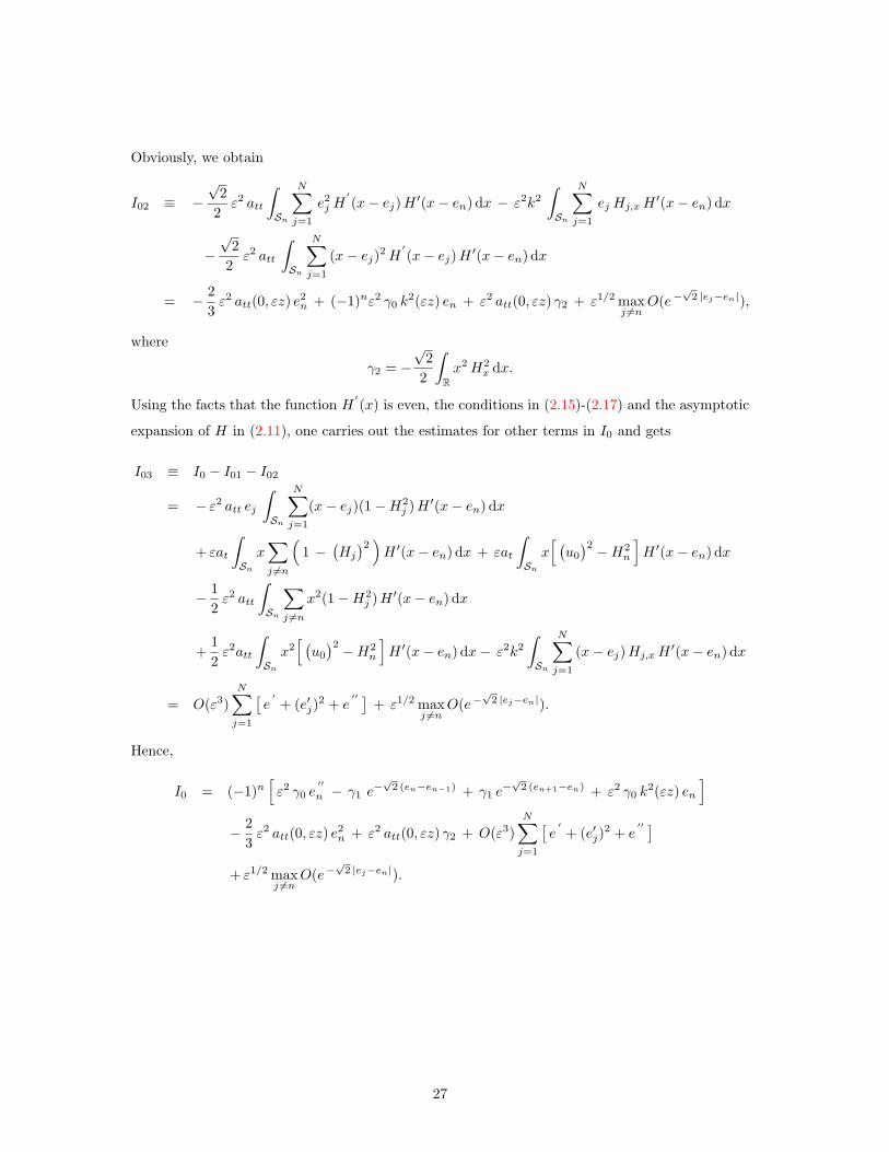
Obviously, we obtain
I02 ≡ −√
22ε2 att
∫Sn
N∑j=1
e2j H
′(x− ej)H ′(x− en) dx − ε2k2
∫Sn
N∑j=1
ej Hj,xH′(x− en) dx
−√
22ε2 att
∫Sn
N∑j=1
(x− ej)2H′(x− ej)H ′(x− en) dx
= − 23ε2 att(0, εz) e2
n + (−1)nε2 γ0 k2(εz) en + ε2 att(0, εz) γ2 + ε1/2 max
j 6=nO(e−
√2 |ej−en|),
where
γ2 = −√
22
∫Rx2H2
x dx.
Using the facts that the function H′(x) is even, the conditions in (2.15)-(2.17) and the asymptotic
expansion of H in (2.11), one carries out the estimates for other terms in I0 and gets
I03 ≡ I0 − I01 − I02
= − ε2 att ej
∫Sn
N∑j=1
(x− ej)(1−H2j )H ′(x− en) dx
+ εat
∫Snx∑j 6=n
(1 −
(Hj
)2 )H ′(x− en) dx + εat
∫Snx[ (u0
)2 −H2n
]H ′(x− en) dx
− 12ε2 att
∫Sn
∑j 6=n
x2(1−H2j )H ′(x− en) dx
+12ε2att
∫Snx2[ (u0
)2 −H2n
]H ′(x− en) dx− ε2k2
∫Sn
N∑j=1
(x− ej)Hj,xH′(x− en) dx
= O(ε3)N∑j=1
[e′+ (e′j)
2 + e′′ ]
+ ε1/2 maxj 6=n
O(e−√
2 |ej−en|).
Hence,
I0 = (−1)n[ε2 γ0 e
′′
n − γ1 e−√
2 (en−en−1) + γ1 e−√
2 (en+1−en) + ε2 γ0 k2(εz) en
]− 2
3ε2 att(0, εz) e2
n + ε2 att(0, εz) γ2 + O(ε3)N∑j=1
[e′+ (e′j)
2 + e′′ ]
+ ε1/2 maxj 6=n
O(e−√
2 |ej−en|).
27

Similarly, we obtain the estimates for the components in I1
I11 ≡ −√
2 ε at∫Sn
N∑j=1
H ′(x− ej) fj H ′(x− en) dx
+√
2 ε2kat
∫Sn
N∑j=1
(−1)j+1 Ψx(x− ej)H ′(x− en) dx
+ 2√
2 ε2a2t
∫Sn
N∑j=1
ej H(x− ej)Ψ(x− ej)H ′(x− en) dx
= − 43ε at(0, εz)fn + ε2 a2
t (0, εz) γ3 en + (−1)n+1ε2 k(εz) at(0, εz) γ4 + O(ε2)N∑j=1
fj ,
where
γ3 = 2√
2∫
RH ΨH
′dx, γ4 =
√2∫
RΨxH
′dx.
Using the facts that the functions H′(x) and φ∗(x, z) are even, we can derive
I12 ≡ − 3 ε∫Sn
N∑j=1
[ (u0
)2 −H2j
]φ∗j H
′(x− en) dx
+ 2√
2 ε2 a2t
∫Sn
N∑j=1
(x− ej)H(x− ej) Ψ(x− ej)H ′(x− en) dx
+ 2√
2 ε2at
∫Sn
N∑j=1
x(u0 −Hj)φ∗j H′(x− en) dx
−∫Sn
[3u0
(φ∗)2 +
(φ∗)3 ]
H ′(x− en) dx
= O(ε3)at(0, εz) + O(ε2)N∑j=1
fj ,
Thus, we finish the estimate of I1.
To compute En2(εz), recall that for (x, z) ∈ Sδ/ε \An,
H ′(x− en) = maxj 6=n
O(e−12 |ej−en|),
and that ηεδE(x, z) = ηεδE1(x, z). Thus we can estimate
En2(εz) = εmaxj 6=n
O(e−|ej−en|) +O(ε1/2)2∑i=1
Ii.
Gathering the above estimates, we get the following, for n = 1, . . . , N∫Sηεδ E(x, z)H ′(x− en(εz)) dx = (−1)n
[ε2 γ0 e
′′
n − γ1 e−√
2 (en−en−1) + γ1 e−√
2 (en+1−en)]
+ (−1)nε2 γ0 k2(εz) en −
23ε2 att(0, εz) e2
n + ε2 att(0, εz) γ2
− 43ε at(0, εz)fn + ε2 a2
t (0, εz) γ3 en
+ (−1)n+1ε2 k(εz)at(0, εz)γ4 + Pn(εz). (6.2)
28

For further references we observe that
||Pn||L2(0,1) ≤ Cε3/2, n = 1, · · · , N. (6.3)
Continuing with other two terms involved in (6.1), using the quadratic nature of the nonlinear
term N2(φ) and Proposition 5.1, we get for
Qn(εz) ≡∫SN2(φ)H ′(x− en(εz)) dx
a similar estimate
||Qn||L2(0,1) ≤ Cε3/2, n = 1, · · · , N. (6.4)
We point out that, by Proposition 5.1, Qn is a continuous function of the parameters f.
The last term in (6.1) can be written as
Vn(εz) ≡∫SL(φ)H ′(x− en(εz)) dx
=∫SφzzH
′(x− en(εz)) dx+∫Sηε10δ B8(φ)H ′(x− en(εz)) dx
+∫Sφ[H ′′′(x− en(εz)) + F
′(W )H ′(x− en(εz))
]dx.
A similar estimate holds
||Vn||L2(0,1) ≤ Cε3/2, n = 1, · · · , N. (6.5)
In fact, the proof is very straightforward. For example, using the orthogonality conditions we can
get
V1n(εz) ≡
∫SφzzH
′(x− en(εz)) dx
= ε2
∫Sφ[e′′
nH′′(x− en(εz))− (e
′
n)2H ′′′(x− en(εz))]
dx
+ 2εe′
n
∫SφzH
′′(x− en(εz)) dx
The estimate for V1n follows from Proposition 5.1. Moreover, it also depends continuously on the
parameters f.
Now, from above discussion, for θ = εz, by the notations of
Mn(θ, f, f′, f′′) ≡ Pn +Qn + Vn, α1(θ) =
43at(0, θ), α3(θ) =
23att(0, θ), (6.6)
α2,n(θ) = − γ0 k2(θ)− (−1)na2
t (0, εz)γ3, α4,n(θ) = − (−1)nγ2 att(0, θ)− γ4 k(θ) at(0, θ), (6.7)
we draw a conclusion as the following proposition:
29

Proposition 6.1. For the validity of (5.16), there should hold the following equations,
ε2 γ0 e′′n − γ1 e
−√
2 (en−en−1) + γ1 e−√
2 (en+1−en) + (−1)n+1 ε α1(θ) fn
− ε2 α2,n(θ) en − (−1)n ε2 α3(θ) e2n = ε2 α4,n(θ) + Mn, n = 1, . . . , N.
Moreover, Mn can be decomposed in the following way
Mn(θ, f, f′, f′′) =Mn1(θ, f, f
′, f′′) + Mn2(θ, f, f
′).
where Mn1 and Mn2 are continuous of their arguments. Function Mn1 satisfies the following
properties, for n = 1, · · · , N
∣∣∣∣Mn1(θ, f, f′, f′′)∣∣∣∣L2(0,1)
≤ Cε3/2,∣∣∣∣Mn1(θ, f, f′, f′′)−Mn1(θ, f1, f
′
1, f′′
1 )∣∣∣∣L2(0,1)
≤ Cε3/2 | log ε|q ||f− f1||H2(0,1).
Function Mn2 satisfies the following estimates for n = 1, · · · , N
∣∣∣∣Mn2(θ, f, f′)∣∣∣∣L2(0,1)
≤ Cε3/2.
We omit the proof of this proposition. In fact, careful examining of all terms will lead the
decomposition of the operator Mn and the properties of its components Mn1 and Mn2.
7 Location and interaction of clustered Layers
Recall that N = 2m+ 1 is a fixed odd integer as in Theorem 1.2. Define the operators by
L∗n(fn) ≡ ε2 γ0 f′′n + ε (−1)n+1 α1(θ) fn − γ1 e
−√
2(fn−fn−1+βn
)+ γ1 e
−√
2(fn+1−fn+βn+1
)− ε2 α5,n(θ) fn − ε2 (−1)n α3(θ) f2
n,
where α5,n and βn are given by
α5,n(θ) = α2,n(θ) + 2α3(θ)f(θ), βn = 2(−1)n+1f,
with f is the function defined in (2.21). α1 is a positive function defined in (6.6). Using the fact
en = fn + (−1)n+1f and Proposition 6.1, after obvious algebra, we have to deal with the following
system, with n running from 1 to N
L∗n(fn) = ε2 α6,n + Mn, f ′n(`) = f ′n(0), fn(`) = fn(0), (7.1)
where f0 = −∞, fN+1 =∞ and the function α6,n is defined by
α6,n(θ) = α4,n(θ) − γ0(−1)n+1f′′(θ) + (−1)n+1α2,n(θ)f(θ) + (−1)nα3(θ)f2(θ).
30
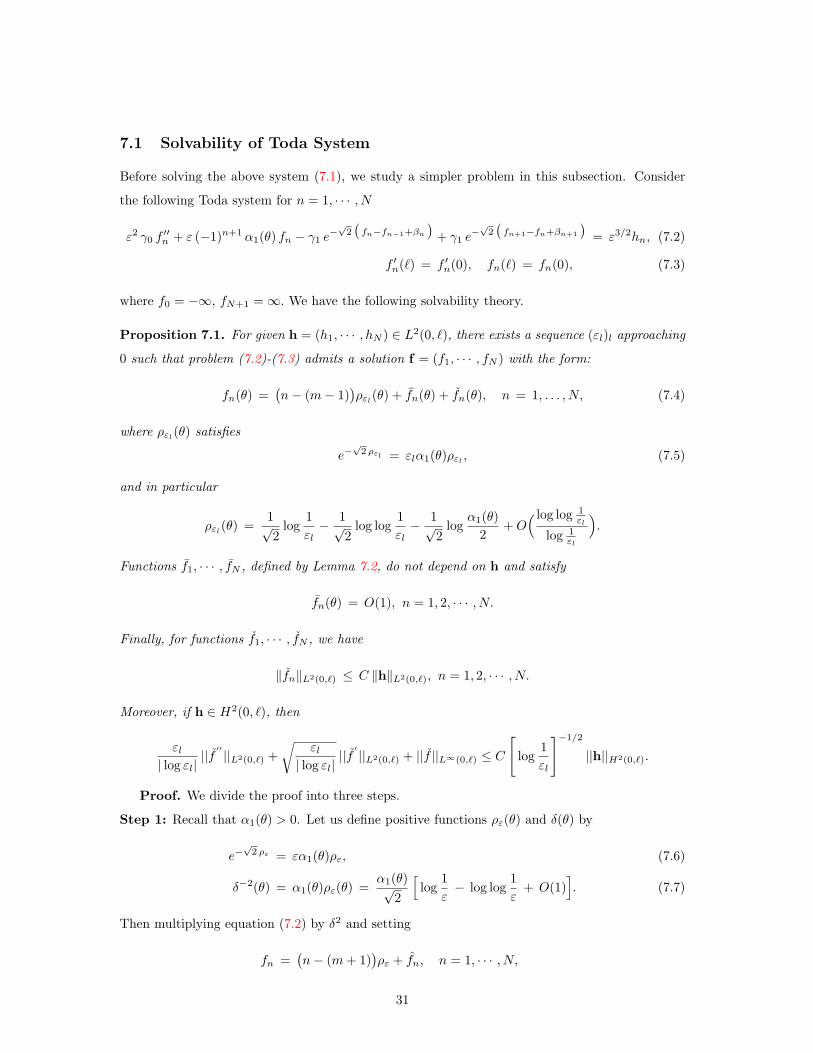
7.1 Solvability of Toda System
Before solving the above system (7.1), we study a simpler problem in this subsection. Consider
the following Toda system for n = 1, · · · , N
ε2 γ0 f′′n + ε (−1)n+1 α1(θ) fn − γ1 e
−√
2(fn−fn−1+βn
)+ γ1 e
−√
2(fn+1−fn+βn+1
)= ε3/2hn, (7.2)
f ′n(`) = f ′n(0), fn(`) = fn(0), (7.3)
where f0 = −∞, fN+1 =∞. We have the following solvability theory.
Proposition 7.1. For given h = (h1, · · · , hN ) ∈ L2(0, `), there exists a sequence (εl)l approaching
0 such that problem (7.2)-(7.3) admits a solution f = (f1, · · · , fN ) with the form:
fn(θ) =(n− (m− 1)
)ρεl(θ) + fn(θ) + fn(θ), n = 1, . . . , N, (7.4)
where ρεl(θ) satisfies
e−√
2 ρεl = εlα1(θ)ρεl , (7.5)
and in particular
ρεl(θ) =1√2
log1εl− 1√
2log log
1εl− 1√
2log
α1(θ)2
+O( log log 1
εl
log 1εl
).
Functions f1, · · · , fN , defined by Lemma 7.2, do not depend on h and satisfy
fn(θ) = O(1), n = 1, 2, · · · , N.
Finally, for functions f1, · · · , fN , we have
‖fn‖L2(0,`) ≤ C ‖h‖L2(0,`), n = 1, 2, · · · , N.
Moreover, if h ∈ H2(0, `), then
εl| log εl|
||f′′||L2(0,`) +
√εl
| log εl|||f′||L2(0,`) + ||f ||L∞(0,`) ≤ C
[log
1εl
]−1/2
||h||H2(0,`).
Proof. We divide the proof into three steps.
Step 1: Recall that α1(θ) > 0. Let us define positive functions ρε(θ) and δ(θ) by
e−√
2 ρε = εα1(θ)ρε, (7.6)
δ−2(θ) = α1(θ)ρε(θ) =α1(θ)√
2
[log
1ε− log log
1ε
+ O(1)]. (7.7)
Then multiplying equation (7.2) by δ2 and setting
fn =(n− (m+ 1)
)ρε + fn, n = 1, · · · , N,
31
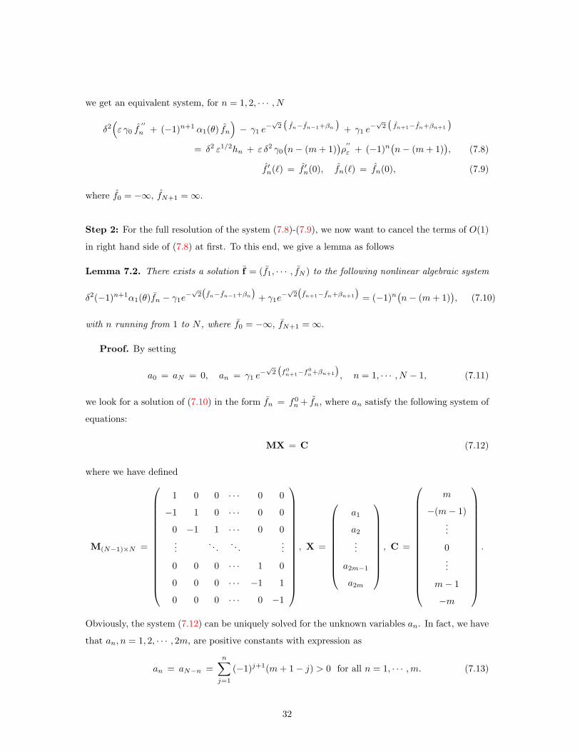
we get an equivalent system, for n = 1, 2, · · · , N
δ2(ε γ0 f
′′
n + (−1)n+1 α1(θ) fn)− γ1 e
−√
2(fn−fn−1+βn
)+ γ1 e
−√
2(fn+1−fn+βn+1
)= δ2 ε1/2hn + ε δ2 γ0
(n− (m+ 1)
)ρ′′
ε + (−1)n(n− (m+ 1)
), (7.8)
f ′n(`) = f ′n(0), fn(`) = fn(0), (7.9)
where f0 = −∞, fN+1 =∞.
Step 2: For the full resolution of the system (7.8)-(7.9), we now want to cancel the terms of O(1)
in right hand side of (7.8) at first. To this end, we give a lemma as follows
Lemma 7.2. There exists a solution f = (f1, · · · , fN ) to the following nonlinear algebraic system
δ2(−1)n+1α1(θ)fn − γ1e−√
2(fn−fn−1+βn
)+ γ1e
−√
2(fn+1−fn+βn+1
)= (−1)n
(n− (m+ 1)
), (7.10)
with n running from 1 to N , where f0 = −∞, fN+1 =∞.
Proof. By setting
a0 = aN = 0, an = γ1 e−√
2(f0n+1−f
0n+βn+1
), n = 1, · · · , N − 1, (7.11)
we look for a solution of (7.10) in the form fn = f0n + fn, where an satisfy the following system of
equations:
MX = C (7.12)
where we have defined
M(N−1)×N =
1 0 0 · · · 0 0
−1 1 0 · · · 0 0
0 −1 1 · · · 0 0...
. . . . . ....
0 0 0 · · · 1 0
0 0 0 · · · −1 1
0 0 0 · · · 0 −1
, X =
a1
a2
...
a2m−1
a2m
, C =
m
−(m− 1)...
0...
m− 1
−m
.
Obviously, the system (7.12) can be uniquely solved for the unknown variables an. In fact, we have
that an, n = 1, 2, · · · , 2m, are positive constants with expression as
an = aN−n =n∑j=1
(−1)j+1(m+ 1− j) > 0 for all n = 1, · · · ,m. (7.13)
32

By (7.11), for n = 1, · · · ,m,m+ 2, · · · , N , functions f0n can be written as
f0n(θ) =
√2
2log
m∏i=n
ai −√
22
(m+ 1− n) log γ1
+ (−1)m[(−1)m+n−1 + 1
]f(θ) + f0
m+1(θ), n = 1, 2, · · · ,m,
f0n(θ) = −
√2
2log
n−1∏i=m+1
ai −√
22
(n−m− 1) log γ1
+ (−1)m[(−1)m+n + 1
]f(θ) + f0
m+1(θ), n = m+ 2,m+ 3, · · · , N.
Hence all functions f0n, n = 1, · · · , N , can be uniquely determined provided that we set
f0m+1(θ) = 4(−1)mf(θ).
Moreover, there holdsN∑n=1
(−1)n+1 f0n = 0. (7.14)
Then functions fn, n = 1, 2, · · · , N , satisfy:
δ2(−1)n+1 α1(θ) fn − an−1
[e−√
2(fn−fn−1
)− 1
]+ an
[e−√
2(fn+1−fn
)− 1
]= − δ2 (−1)n+1 α1(θ) f0
n, (7.15)
where f0 = −∞, fN+1 =∞.
Notice that the right hand of (7.15) is of order O(δ2) now. This however is not enough to
solve our nonlinear problem since there is a term of the same order in front of the linear part of
the operator. Thus we need to find one more term in the expansion of fn to cancel the terms
δ2 (−1)n+1α1 f0n, n = 1, 2, · · · , N . To this end let fn = fn + f1
n where f1n, n = 1, . . . , N , solve the
following system of equations:
√2 Af1 = α h with α = δ2α1(θ), (7.16)
where
A =
a1 −a1 0 0 · · · 0 0 0 0
−a1 (a1 + a2) −a2 0 · · · 0 0 0 0...
. . ....
0 0 0 0 · · · 0 −a2m−1 (a2m−1 + a2m) −a2m
0 0 0 0 · · · 0 0 −a2m a2m
, (7.17)
33

and
J(α) =
α 0 · · · 0 0
0 −α · · · 0 0. . .
0 0 · · · −α 0
0 0 · · · 0 α
, f1 =
f1
1
...
f1N
, h =
f01
−f02
...
−f02m
f0N
. (7.18)
The matrix A has only one zero eigenvalue with corresponding eigenvector (1, 1, · · · , 1)T . The
system (7.16) can be solved due to the formula (7.14). It is easy to derive that the term f1 is small
in the order of O(| log ε|−1).
Now, fn, n = 1, · · · , N , solve the following nonlinear system of equations,
δ2(−1)n+1 α1(θ) fn +√
2 an−1
(fn − fn−1
)−√
2 an(fn+1 − fn
)= − δ2 (−1)n+1 α1 f
1n + Nn(f , f1), (7.19)
where Nn, n = 1, · · · , N , are given by
Nn(f , f1) = an−1
[e−√
2 (fn−fn−1+f1n−f
1n−1) − 1 +
√2 (fn − fn−1) +
√2 (f1
n − f1n−1)
]− an
[e−√
2 (fn+1−fn+f1n+1−f
1n) − 1 +
√2 (fn+1 − fn) +
√2 (f1
n+1 − f1n)],
and f0 = −∞, fN+1 = ∞. In order to use fixed point argument to solve (7.19), we consider the
following system of equations:
(√2A + J
)f = αh with α = δ2α1(θ), (7.20)
where the matrix J is defined in (7.18). The system (7.20) has a uniformly (with respect to ε)
bounded solution due to the following fact:
det(√
2A + J(α))
= (−1)m αN + · · · +(
ΠNj=1
√2 aj
)α.
We claim that problem (7.19) can be solved by a contraction mapping principle in the set
X =
‖f‖L2(0,`) ≤
1(log 1
ε
)1+σ
with small constant σ > 0.
In fact, from the smallness of f1 in X, we have
‖N(f , f1)‖L2(0,`) ≤C
| log ε|1+2σ.
The result of Lemma 7.2 follows by a straightforward argument.
34
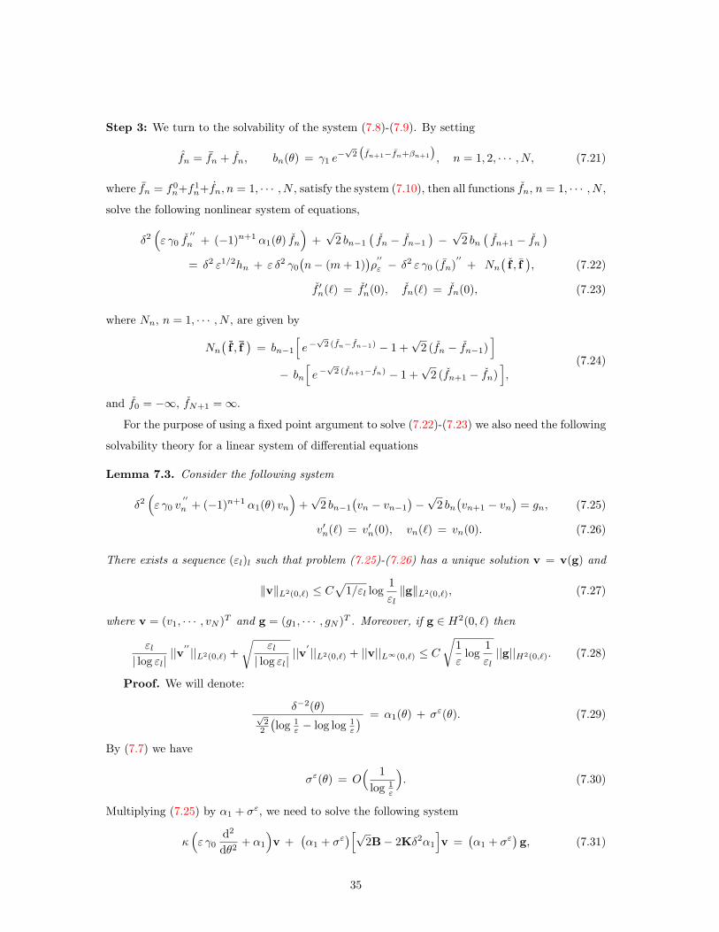
Step 3: We turn to the solvability of the system (7.8)-(7.9). By setting
fn = fn + fn, bn(θ) = γ1 e−√
2(fn+1−fn+βn+1
), n = 1, 2, · · · , N, (7.21)
where fn = f0n+f1
n+fn, n = 1, · · · , N , satisfy the system (7.10), then all functions fn, n = 1, · · · , N ,
solve the following nonlinear system of equations,
δ2(ε γ0 f
′′
n + (−1)n+1 α1(θ) fn)
+√
2 bn−1
(fn − fn−1
)−√
2 bn(fn+1 − fn
)= δ2 ε1/2hn + ε δ2 γ0
(n− (m+ 1)
)ρ′′
ε − δ2 ε γ0 (fn)′′
+ Nn(f , f), (7.22)
f ′n(`) = f ′n(0), fn(`) = fn(0), (7.23)
where Nn, n = 1, · · · , N , are given by
Nn(f , f)
= bn−1
[e−√
2 (fn−fn−1) − 1 +√
2 (fn − fn−1)]
− bn
[e−√
2 (fn+1−fn) − 1 +√
2 (fn+1 − fn)],
(7.24)
and f0 = −∞, fN+1 =∞.
For the purpose of using a fixed point argument to solve (7.22)-(7.23) we also need the following
solvability theory for a linear system of differential equations
Lemma 7.3. Consider the following system
δ2(ε γ0 v
′′
n + (−1)n+1 α1(θ) vn)
+√
2 bn−1
(vn − vn−1
)−√
2 bn(vn+1 − vn
)= gn, (7.25)
v′n(`) = v′n(0), vn(`) = vn(0). (7.26)
There exists a sequence (εl)l such that problem (7.25)-(7.26) has a unique solution v = v(g) and
‖v‖L2(0,`) ≤ C√
1/εl log1εl‖g‖L2(0,`), (7.27)
where v = (v1, · · · , vN )T and g = (g1, · · · , gN )T . Moreover, if g ∈ H2(0, `) then
εl| log εl|
||v′′||L2(0,`) +
√εl
| log εl|||v′||L2(0,`) + ||v||L∞(0,`) ≤ C
√1ε
log1εl||g||H2(0,`). (7.28)
Proof. We will denote:
δ−2(θ)√
22
(log 1
ε − log log 1ε
) = α1(θ) + σε(θ). (7.29)
By (7.7) we have
σε(θ) = O( 1
log 1ε
). (7.30)
Multiplying (7.25) by α1 + σε, we need to solve the following system
κ(ε γ0
d2
dθ2+ α1
)v +
(α1 + σε
)[√2B− 2Kδ2α1
]v =
(α1 + σε
)g, (7.31)
35
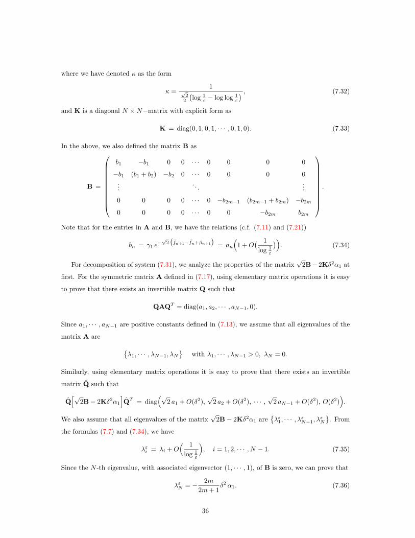
where we have denoted κ as the form
κ =1
√2
2
(log 1
ε − log log 1ε
) , (7.32)
and K is a diagonal N ×N−matrix with explicit form as
K = diag(0, 1, 0, 1, · · · , 0, 1, 0). (7.33)
In the above, we also defined the matrix B as
B =
b1 −b1 0 0 · · · 0 0 0 0
−b1 (b1 + b2) −b2 0 · · · 0 0 0 0...
. . ....
0 0 0 0 · · · 0 −b2m−1 (b2m−1 + b2m) −b2m0 0 0 0 · · · 0 0 −b2m b2m
.
Note that for the entries in A and B, we have the relations (c.f. (7.11) and (7.21))
bn = γ1 e−√
2(fn+1−fn+βn+1
)= an
(1 +O
( 1log 1
ε
)). (7.34)
For decomposition of system (7.31), we analyze the properties of the matrix√
2B− 2Kδ2α1 at
first. For the symmetric matrix A defined in (7.17), using elementary matrix operations it is easy
to prove that there exists an invertible matrix Q such that
QAQT = diag(a1, a2, · · · , aN−1, 0).
Since a1, · · · , aN−1 are positive constants defined in (7.13), we assume that all eigenvalues of the
matrix A are λ1, · · · , λN−1, λN
with λ1, · · · , λN−1 > 0, λN = 0.
Similarly, using elementary matrix operations it is easy to prove that there exists an invertible
matrix Q such that
Q[√
2B− 2Kδ2α1
]QT = diag
(√2 a1 +O(δ2),
√2 a2 +O(δ2), · · · ,
√2 aN−1 +O(δ2), O(δ2)
).
We also assume that all eigenvalues of the matrix√
2B− 2Kδ2α1 areλε1, · · · , λεN−1, λ
εN
. From
the formulas (7.7) and (7.34), we have
λεi = λi +O( 1
log 1ε
), i = 1, 2, · · · , N − 1. (7.35)
Since the N -th eigenvalue, with associated eigenvector (1, · · · , 1), of B is zero, we can prove that
λεN = − 2m2m+ 1
δ2 α1. (7.36)
36

Moreover, since√
2B − 2Kδ2α1 is a symmetric matrix, there exists another invertible matrix P
such that
P(√
2B− 2Kδ2α1
)P−1 = diag(λε1, · · · , λεN ).
Now, after setting two new vectors
u = (u1, · · · , uN )T = Pv, g = (g1, · · · , gN )T =(α1 + σε
)Pg,
system (7.31) is equivalent to the following system with suitable periodic boundary conditions,
κ(ε γ0
d2
dθ2u + α1u
)+ κ ε γ0P
d2P−1
dθu + 2κ ε γ0P
dP−1
dθu
+ diag(λε1, · · · , λεN )(α1 + σε
)u = g. (7.37)
Hence, we need to consider the systems, as follows, with suitable periodic boundary conditions.
One describes the location of the center of mass of N−interfaces as
κ(ε γ0
d2
dθ2uN + α1uN
)+ λεN
(α1 + σε
)uN = gN , (7.38)
and the other relate to the balance of mutual interaction of N -interfaces as
κ(ε γ0
d2
dθ2ui + α1ui
)+ λεi
(α1 + σε
)ui = gi, i = 1, 2, · · · , N − 1. (7.39)
Firstly, using formulas (7.29), (7.32) and (7.36), problem (7.38) read as
ε γ0d2
dθ2uN +
α1
2m+ 1uN =
1κ
gN , (7.40)
with suitable periodic boundary conditions, which can be solved by the following claim.
Claim 1: If g ∈ L2(0, `) then for all small ε satisfying the gap condition: given c > 0, there exists
ε0 > 0 such that for all ε < ε0 satisfying the gap condition∣∣∣j2ε− λ∗N
∣∣∣ ≥ c√ε for all j ∈ N, (7.41)
there is a unique solution uN ∈ H2(0, `) to problem (7.40) which satisfies
ε||uN′′||L2(0,`) + ||uN ||L∞(0,`) ≤ Cε−1/2 log
1ε||gN ||H2(0,`).
Moreover, if gN ∈ H2(0, `) then
ε||uN′′||L2(0,`) + ||uN ||L∞(0,`) ≤ C log
1ε||gN ||H2(0,`).
For proof of this Claim, the reader can refer to Lemma 8.1 in [15].
Secondly, for the solvability theory of equations in (7.39), define linear operators by
Liε = κ(ε γ0
d2
dθ2+ α1
)+ λεi
(α1 + σε
), i = 1, 2, · · · , N − 1.
37
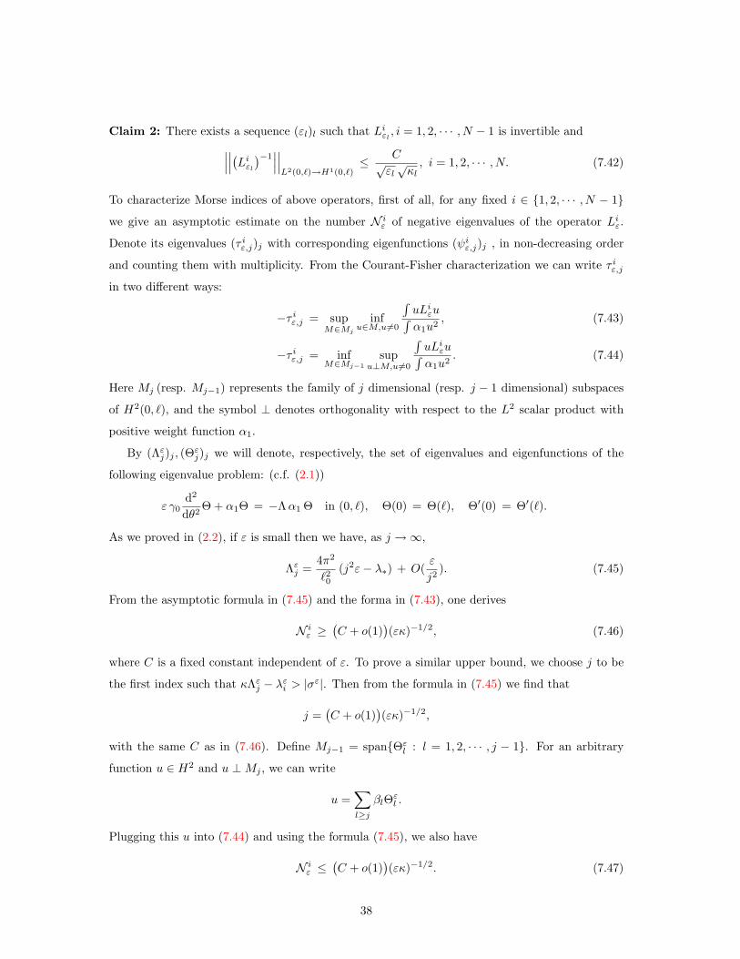
Claim 2: There exists a sequence (εl)l such that Liεl , i = 1, 2, · · · , N − 1 is invertible and∣∣∣∣∣∣(Liεl)−1∣∣∣∣∣∣L2(0,`)→H1(0,`)
≤ C√εl√κl, i = 1, 2, · · · , N. (7.42)
To characterize Morse indices of above operators, first of all, for any fixed i ∈ 1, 2, · · · , N − 1
we give an asymptotic estimate on the number N iε of negative eigenvalues of the operator Liε.
Denote its eigenvalues (τ iε,j)j with corresponding eigenfunctions (ψiε,j)j , in non-decreasing order
and counting them with multiplicity. From the Courant-Fisher characterization we can write τ iε,j
in two different ways:
−τ iε,j = supM∈Mj
infu∈M,u6=0
∫uLiεu∫α1u2
, (7.43)
−τ iε,j = infM∈Mj−1
supu⊥M,u6=0
∫uLiεu∫α1u2
. (7.44)
Here Mj (resp. Mj−1) represents the family of j dimensional (resp. j − 1 dimensional) subspaces
of H2(0, `), and the symbol ⊥ denotes orthogonality with respect to the L2 scalar product with
positive weight function α1.
By (Λεj)j , (Θεj)j we will denote, respectively, the set of eigenvalues and eigenfunctions of the
following eigenvalue problem: (c.f. (2.1))
ε γ0d2
dθ2Θ + α1Θ = −Λα1 Θ in (0, `), Θ(0) = Θ(`), Θ′(0) = Θ′(`).
As we proved in (2.2), if ε is small then we have, as j →∞,
Λεj =4π2
`20(j2ε− λ∗) + O(
ε
j2). (7.45)
From the asymptotic formula in (7.45) and the forma in (7.43), one derives
N iε ≥
(C + o(1)
)(εκ)−1/2, (7.46)
where C is a fixed constant independent of ε. To prove a similar upper bound, we choose j to be
the first index such that κΛεj − λεi > |σε|. Then from the formula in (7.45) we find that
j =(C + o(1)
)(εκ)−1/2,
with the same C as in (7.46). Define Mj−1 = spanΘεl : l = 1, 2, · · · , j − 1. For an arbitrary
function u ∈ H2 and u ⊥Mj , we can write
u =∑l≥j
βlΘεl .
Plugging this u into (7.44) and using the formula (7.45), we also have
N iε ≤
(C + o(1)
)(εκ)−1/2. (7.47)
38
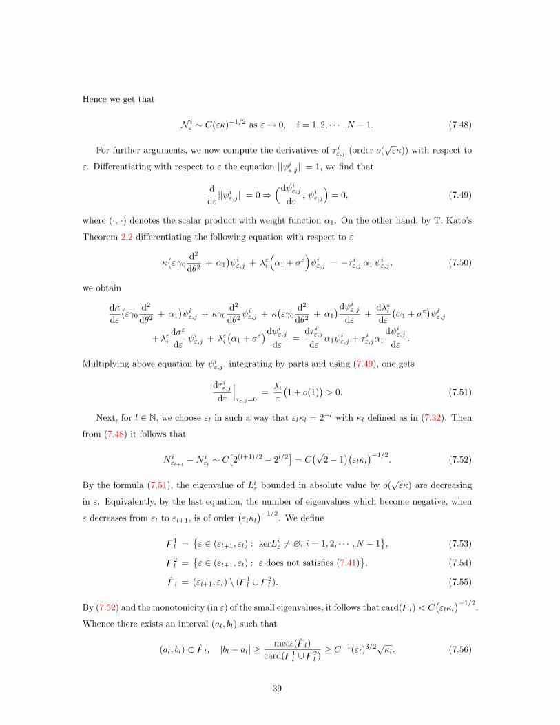
Hence we get that
N iε ∼ C(εκ)−1/2 as ε→ 0, i = 1, 2, · · · , N − 1. (7.48)
For further arguments, we now compute the derivatives of τ iε,j (order o(√εκ)) with respect to
ε. Differentiating with respect to ε the equation ||ψiε,j || = 1, we find that
ddε||ψiε,j || = 0⇒
(dψiε,jdε
, ψiε,j
)= 0, (7.49)
where (·, ·) denotes the scalar product with weight function α1. On the other hand, by T. Kato’s
Theorem 2.2 differentiating the following equation with respect to ε
κ(ε γ0
d2
dθ2+ α1
)ψiε,j + λεi
(α1 + σε
)ψiε,j = −τ iε,j α1 ψ
iε,j , (7.50)
we obtain
dκdε(εγ0
d2
dθ2+ α1
)ψiε,j + κγ0
d2
dθ2ψiε,j + κ
(εγ0
d2
dθ2+ α1
)dψiε,jdε
+dλεidε(α1 + σε
)ψiε,j
+λεidσε
dεψiε,j + λεi
(α1 + σε
)dψiε,jdε
=dτ iε,jdε
α1ψiε,j + τ iε,jα1
dψiε,jdε
.
Multiplying above equation by ψiε,j , integrating by parts and using (7.49), one gets
dτ iε,jdε
∣∣∣τε,j=0
=λiε
(1 + o(1)
)> 0. (7.51)
Next, for l ∈ N, we choose εl in such a way that εlκl = 2−l with κl defined as in (7.32). Then
from (7.48) it follows that
N iεl+1−N i
εl∼ C
[2(l+1)/2 − 2l/2
]= C
(√2− 1
)(εlκl
)−1/2. (7.52)
By the formula (7.51), the eigenvalue of Liε bounded in absolute value by o(√εκ) are decreasing
in ε. Equivalently, by the last equation, the number of eigenvalues which become negative, when
ε decreases from εl to εl+1, is of order(εlκl
)−1/2. We define
z1l =
ε ∈ (εl+1, εl) : kerLiε 6= ∅, i = 1, 2, · · · , N − 1
, (7.53)
z2l =
ε ∈ (εl+1, εl) : ε does not satisfies (7.41)
, (7.54)
zl = (εl+1, εl) \ (z1l ∪z2
l ). (7.55)
By (7.52) and the monotonicity (in ε) of the small eigenvalues, it follows that card(zl) < C(εlκl
)−1/2.
Whence there exists an interval (al, bl) such that
(al, bl) ⊂ zl, |bl − al| ≥meas(zl)
card(z1l ∪z2
l )≥ C−1(εl)3/2√κl. (7.56)
39

Hence, by setting εlκl = (al + bl)/2 and using (7.51), we conclude that Liεl , i = 1, 2, · · · , N − 1 is
invertible and ∣∣∣∣∣∣(Liεl)−1∣∣∣∣∣∣L2(0,`)→H1(0,`)
≤ C√εl√κl, i = 1, 2, · · · , N − 1. (7.57)
This completes the proof of Claim 2.
As a consequence of the last two claims and an obvious contraction mapping theory, the solution
to (7.37) exists and satisfies
‖u‖L2(0,`) ≤ C√
1/εl log1εl‖g‖L2(0,`). (7.58)
From (7.58) by a standard argument one can show
11εl
log 1εl
‖u′′‖L2(0,`) +
1√1εl
log 1εl
‖u′‖L2(0,`) + ‖u‖L2(0,`) ≤ C
√1/εl log
1εl‖g‖L2(0,`).
The estimates (7.27) and (7.28) are also a direct consequence.
By using Lemma 7.3, let v = (v1, · · · , vn) be the solution to the problem (7.25)-(7.26) with
right hand side replaced by the following term
δ2 ε1/2hn + ε δ2 γ0
(n− (m+ 1)
)ρ′′
ε − δ2 ε γ0 (fn)′′.
Then problem (7.22)-(7.23) can be solved by a contraction mapping principle in the set
X =
f ∈ H2(0, 1)
∣∣∣∣∣∣ 1√1ε log 1
ε
‖f′‖L2(0,`) + ‖f‖L2(0,`) ≤ ε1/2+σ
.
In fact, in X we have
‖N(f , f)‖L2(0,`) ≤ ε1+2σ.
Now, the result follows by a straightforward argument using Lemma 7.3. The proof of the Propo-
sition 7.1 is complete.
7.2 Proof of Theorem 1.2
In the final part of this section, we solve the system (7.1), which will give a proof of Theorem 1.2.
Proof of Theorem 1.1: Define
D =
f ∈ H2(0, 1)∣∣∣ ‖f‖H2(0,1) ≤ D| log ε|%
with small constant 0 < % < 1 and for given f ∈ D, we can set for n = 1, · · · , N
ε3/2hn(f) ≡ ε2 α6,n(θ) + Mn1(f , f′, f′′) + ε2 α5,n(θ) fn + ε2 (−1)n α3(θ) f 2
n + Mn2(f , f′).
40

For any f3, we can use Proposition 7.1 to get
f4 = T1
(ε3/2h1(f3), · · · , ε3/2hN (f3)
).
Whence, by the fact that Mn1 are contractions on D, making use of the theory developed in
Proposition 7.1 and the Contraction Mapping theorem, we find f for a fixed f in D. This way we
define a mapping as
Z(f) = (f),
and the solution of our problem is simply a fixed point of Z. Continuity of Mn2 with respect to
its parameters and a standard regularity arguments allows us to conclude that Z is compact as
mapping from H1(0, 1) into itself. The Schauder Theorem applies to yield the existence of a fixed
point of Z as required. This ends the proof of Theorem 1.2.
References
[1] N. D. Alikakos and P. W. Bates, On the singular limit in a phase field model of phase transi-
tions, Ann. Inst. H. Poincare Anal. Non Lineaire 5 (1988), no. 2, 141-178.
[2] N. D. Alikakos, P. W. Bates and X. Chen, Periodic traveling waves and locating oscillating
patterns in multidimensional domains, Trans. Amer. Math. Soc. 351 (1999), no. 7, 2777-2805.
[3] N. D. Alikakos, P. W. Bates and G. Fusco, Solutions to the nonautonomous bistable equation
with specified Morse index, I. Existence, Trans. Amer. Math. Soc. 340 (1993), no. 2, 641-654.
[4] N. D. Alikakos, X. Chen and G. Fusco, Motion of a droplet by surface tension along the
boundray, Cal. Var. PDE 11 (2000), 233-306.
[5] N. D. Alikakos and H. C. Simpson, A variational approach for a class of singular perturbation
problems and applications, Proc. Roy. Soc. Edinburgh Sect. A 107 (1987), no. 1-2, 27-42.
[6] S. Allen and J. W. Cahn, A microscopic theory for antiphase boundary motion and its appli-
cation to antiphase domain coarsening, Acta. Metall. 27 (1979), 1084-1095.
[7] S. Angenent, J. Mallet-Paret and L. A. Peletier, Stable transition layers in a semilinear bound-
ary value problem, J. Differential Equations 67 (1987), 212-242.
[8] G. Birkhoff and Gian-Carlo Rota, Ordinary differential equations, Ginn and company, New
York, 1962.
[9] L. Bronsard and B. Stoth, On the existence of high multiplicity interfaces, Math. Res. Lett. 3
(1996), 117-131.
41

[10] E. N. Dancer and S. Yan, Multi-layer solutions for an elliptic problem, J. Diff. Eqns. 194
(2003), 382-405.
[11] E. N. Dancer and S. Yan, Construction of various types of solutions for an elliptic problem,
Calc. Var. Partial Differential Equations 20 (2004), no.1, 93-118.
[12] M. del Pino, Layers with nonsmooth interface in a semilinear elliptic problem, Comm. Partial
Differential Equations 17 (1992), no. 9-10, 1695-1708.
[13] M. del Pino, Radially symmetric internal layers in a semilinear elliptic system, Trans. Amer.
Math. Soc. 347 (1995), no. 12, 4807-4837.
[14] M. del Pino, M. Kowalczyk and J. Wei, Concentration on curves for nonlinear Schrodinger
equations, Comm. Pure Appl. Math. 70 (2007), 113-146.
[15] M. del Pino, M. Kowalczyk and J. Wei, Resonance and interior layers in an inhomogeneous
phase transition model, SIAM J. Math. Anal. 38 (2007), no.5, 1542-1564.
[16] M. del Pino, M. Kowalczyk and J. Wei, The Toda system and clustering interface in the
Allen-Cahn equation, Arch. Ration. Mech. Anal. , 190 (2008), no. 1, 141-187.
[17] M. del Pino, M. Kowalczyk, J. Wei and J. Yang, Interface foliation near minimal submanifolds
in Riemannian manifolds with positive Ricci curvature, submitted 2009.
[18] A. S. do Nascimento, Stable transition layers in a semilinear diffusion equation with spatial
inhomogeneities in N -dimensional domains, J. Differential Equations 190 (2003), no. 1, 16-38.
[19] Y. Du and K. Nakashima, Morse index of layered solutions to the heterogeneous Allen-Cahn
equation, J. Differential Equations 238 (2007), no. 1, 87-117.
[20] Y. Du, The heterogeneous Allen-Cahn equation in a ball: solutions with layers and spikes, J.
Differential Equations 244 (2008), no. 1, 117-169.
[21] P. C. Fife, Boundary and interior transition layer phenomena for pairs of second-order differ-
ential equations, J. Math. Anal. Appl. 54 (1976), no. 2, 497-521.
[22] P. C. Fife and M. W. Greenlee, Interior transition Layers of elliptic boundary value problem
with a small parameter, Russian Math. Survey 29 (1974), no. 4, 103-131.
[23] G. Flores and P. Padilla, Higher energy solutions in the theory of phase trasitions: a variational
approach, J. Diff. Eqns. 169 (2001), 190-207.
42

[24] C. Gui and J. Wei, Multiple interior peak solutions for some singularly perturbed Neumann
problems, J. Diff. Eqns. 158 (1999), no. 1, 1-27.
[25] J. Hale and K. Sakamoto, Existence and stability of transition layers, Japan J. Appl. Math. 5
(1988), no. 3, 367-405.
[26] T. Kato, Perturbation theory for linear operators, Classics in Mathematics. Springer-Verlag,
Berlin, 1995.
[27] R.V. Kohn and P. Sternberg, Local minimizers and singular perturbations, Proc. Royal Soc.
Edinburgh 11A (1989), 69-84.
[28] M. Kowalczyk, On the existence and Morse index of solutions to the Allen-Cahn equation in
two dimensions, Ann. Mat. Pura Appl. (4) 184 (2005), no. 1, 17-52.
[29] B. M. Levitan and I. S. Sargsjan, Sturm-Liouville and Dirac operator. Mathematics and its
application (Soviet Series), 59. Kluwer Acadamic Publishers Group, Dordrecht, 1991.
[30] F. Mahmoudi, A. Malchiodi and J. Wei, Transition Layer for the Heterogeneous Allen-Cahn
Equation, Ann. Inst. H. Poincar Anal. Non Linaire 25 (2008), no. 3, 609-631.
[31] A. Malchiodi, W.-M. Ni and J. Wei, Boundary clustered interfaces for the Allen-Cahn equa-
tion, Pacific J. Math. 229 (2007), No. 2, 447-468.
[32] A. Malchiodi and J. Wei, Boundary interface for the Allen-Cahn equation, J. Fixed Point
Theory Appl. 1 (2007), no. 2, 305-336.
[33] L. Modica, The gradient theory of phase transitions and the minimal interface criterion, Arch.
Rat. Mech. Anal. 98 (1987), 357-383.
[34] K. Nakashima, Multi-layered stationary solutions for a spatially inhomogeneous Allen-Cahn
equation, J. Diff. Eqns. 191 (2003), 234-276.
[35] K. Nakashima and K. Tanaka, Clustering layers and boundary layers in spatially inhomoge-
neous phase transition problems, Ann. Inst. H. Poincare Anal. NonLineaire 20 (2003), no. 1,
107-143.
[36] Y. Nishiura and H. Fujii, Stability of singularly perturbed solutions to systems of reaction–
diffusion equations, SIAM J. Math. Anal. 18 (1987), 1726-1770.
[37] F. Pacard and M. Ritore, From constant mean curvature hypersurfaces to the gradient theory
of phase transitions, J. Diff. Geom. 64 (2003), 359-423.
43

[38] P. Padilla and Y. Tonegawa, On the convergence of stable phase transitions, Comm. Pure
Appl. Math. 51 (1998), 551-579.
[39] P. H. Rabinowitz and E. Stredulinsky, Mixed states for an Allen-Cahn type equation, I, Comm
Pure Appl. Math. 56 (2003), 1078-1134.
[40] P. H. Rabinowitz and E. Stredulinsky, Mixed states for an Allen-Cahn type equation, II, Calc.
Var. Partial Differential Equations 21 (2004), 157-207.
[41] K. Sakamoto, Construction and stability an alysis of transition layer solutions in reaction-
diffusion systems, Tohoku Math. J. (2) 42 (1990), no. 1, 17-44.
[42] K. Sakamoto, Infinitely many fine modes bifurcating from radially symmetric internal layers,
Asymptot. Anal. 42 (2005), no. 1-2, 55-104.
[43] P. Sternberg and K. Zumbrun, Connectivity of phase boundaries in strictly convex domains,
Arch. Rational Mech. Anal. 141 (1998), no. 4, 375-400.
[44] J. Wei and J. Yang, Solutions with transition layer and spike in an inhomogeneous phase
transition model, Journal of Differential Equations 246(2009), no.9, 3642-3667.
44