to freak out or to chill out? a guide to model monitoring · what is model monitoring? model...

© 2014 Finity Consulting Pty Limited

To freak out or to chill out?

A guide to model monitoring

John Yick & Michael McLean

Finity Personal Lines Pricing

and Portfolio Management Seminar

22 May 2014

Contents

Introduction

Change detection indicators

Model performance measures

Case study: sales models

Other considerations

Key points

2

Introduction

What is model monitoring?

Model performance can go down (or break down) over time no

matter how good a model is

Model monitoring is about

Seeing how model predictions are performing against actual

recent experience as they emerge

It is NOT about how well the models fits a static set of data

(that is used to build the model)

4

Actual and Expected

Exposure Actual Rate Predicted Rate

Model Build Monitoring

Why Monitor

5

Use of Price Optimisation

Sophistication of price practice in

the market

Increase in number of and complexity of

models

More resources

required to maintain the

models

Obtain timely warning if models

are no longer working well

Focus resources on models required

fixing (not rebuild every model)

Provide governance and audit trails for managing technical

models

Change detection indicators

How to decide if there is a change

Suppose we are looking at some average claim size over a 24 month

period and wish to know if the average claim sizes have shifted

7

3000

3100

3200

3300

3400

3500

3600

3700

1 2 3 4 5 6 7 8 9 10 11 12 13 14 15 16 17 18 19 20 21 22 23 24

Average Claim size by Month

Actual

Magnitude of difference from expectation

– A/E Can look at the difference between

the monthly average and some

expectation

The idea is to see when it

breaches certain Upper/Lower

confidence limits (UCL/LCL)

Using expectations (rather than

simple historical average) can deal

with issues such as seasonality,

change in claims mix etc.

8

3000

3100

3200

3300

3400

3500

3600

3700

1 2 3 4 5 6 7 8 9 10 11 12 13 14 15 16 17 18 19 20 21 22 23 24

Average Claim size by Month

Mean+ 3 StDev Mean - 3 StDev Actual

88%90%92%94%96%98%

100%102%104%106%108%

1 2 3 4 5 6 7 8 9 10 11 12 13 14 15 16 17 18 19 20 21 22 23 24

Actual vs Expected by Month

100% + 3 StDev 100% - 3 StDev Act/Exp

Frequency of direction

We can ask: What are the chances

of seeing the number of times the

average claim size being

above/below expectation?

Should see claim size being above

expectation half the time (thanks to

central limit theorem in this case)

We can calculate probability of

seeing the number of outcomes

being above/below average over a

running window (9 months say) –

Sign Test

9

3250

3300

3350

3400

3450

3500

3550

1 2 3 4 5 6 7 8 9 10 11 12 13 14 15 16 17 18 19 20 21 22 23 24

Observed Average Claim size

-1

0

1

2

1 2 3 4 5 6 7 8 9 10 11 12 13 14 15 16 17 18 19 20 21 22 23 24

Signs

Magnitude or frequency?

Take 100k Motor Collision claims

Randomly select between 4,500 to 5,000

claims each month over a period of 24

Months

Inflate claims by 5% for months 13 to 24

Repeat the process 1,000 times

Compare the number of times the shift has

been identified by the 2 different approaches

(using the same probability cut off of 0.5%)

10

A case of power versus speed?

Very few cases being detected for

the first 12 months (where there is

no change)

A/E detects the change quickly but

less than half the time

Sign test takes much longer and

detects it more often

11

0.0%

20.0%

40.0%

60.0%

80.0%

100.0%

1 2 3 4 5 6 7 8 9 10 11 12 13 14 15 16 17 18 19 20 21 22 23 24

Probability of detection by Month - 5% inc

Confidence interval Sign Test

Is there an alternative?

The first approach looks at the magnitude for an individual month’s

experience against some expectation

The second approach looks at the direction of the experience

against some expectation for a number of months

How about combining them?

12

?

Cumulative Sum - CUMSUM

Sum differences between observed

outcome and expectation

Differences would centre around

zero if there is no change but would

bias up/down if some change has

occurred

Usually works better if some function

is applied to give more weight to

more recent months

13

3250

3300

3350

3400

3450

3500

3550

1 2 3 4 5 6 7 8 9 10 11 12 13 14 15 16 17 18 19 20 21 22 23 24

Observed Average Claim size

-250-200-150-100

-500

50100150200250

1 2 3 4 5 6 7 8 9 10 11 12 13 14 15 16 17 18 19 20 21 22 23 24

Cumulative Sum of Difference

Can CUMSUM do better?

Repeat simulation test again – With a logistic weighting function applied to

CUMSUM

Always out performs Sign test

Catches up to A/E by 3rd month after change is introduced

14

0%

20%

40%

60%

80%

100%

1 2 3 4 5 6 7 8 9 10 11 12 13 14 15 16 17 18 19 20 21 22 23 24


Confidence interval Sign Test CUMSUM

Different size shifts

A/E higher chances of detecting change early if shift is large

CUMSUM usually catches up by 3rd month

Sign test always slow to react 15

0%

20%

40%

60%

80%

100%

1 2 3 4 5 6 7 8 9 10 11 12 13 14 15 16 17 18 19 20 21 22 23 24



0%

20%

40%

60%

80%

100%

1 2 3 4 5 6 7 8 9 10 11 12 13 14 15 16 17 18 19 20 21 22 23 24



0%

20%

40%

60%

80%

100%

1 2 3 4 5 6 7 8 9 10 11 12 13 14 15 16 17 18 19 20 21 22 23 24

Probability of detection by Month - 7.5% inc


0%

20%

40%

60%

80%

100%

1 2 3 4 5 6 7 8 9 10 11 12 13 14 15 16 17 18 19 20 21 22 23 24



How about trends?

16

All approaches needs quite awhile to detect the change

CUMSUM seems to be the best performer

0%

10%

20%

30%

40%

50%

60%

70%

1 2 3 4 5 6 7 8 9 10 11 12 13 14 15 16 17 18 19 20 21 22 23 24

Probability of detection - 0.25% inc per Month


0%

20%

40%

60%

80%

100%

1 2 3 4 5 6 7 8 9 10 11 12 13 14 15 16 17 18 19 20 21 22 23 24

Probability of detection - 0.5% inc per Month


• Confidence Intervals and Sign Tests

can give different perspectives

• Combine features from both to get a

more robust measure

• Best to have multiple indicators.

Model fit measures

Looking at aggregate A/E alone is not enough

When assessing model fit we need to think about

How close are the predictions

Need to look beyond the overall level – otherwise

just using the mean (not the best model in most

cases) will achieve that

How good are the ordering of the predictions

Model structure is appropriate (distribution

assumptions etc.) – less important for monitoring

There are quite a number of model fit measures aside from

actual versus expected

19

Deviance

Sort of a measure of distance between actual and predicted

-2 times the log-likelihood ratio of the fitted model compared

to the full model

Equivalent to sum of squared residuals in linear regression

Smaller is better (i.e., predicted values closer to actual

values)

20

𝑫 𝒚 = −𝟐(𝐥𝐨𝐠(𝒑(𝒚|𝜽 𝟎)) – log(p(y| 𝜽 𝒔))

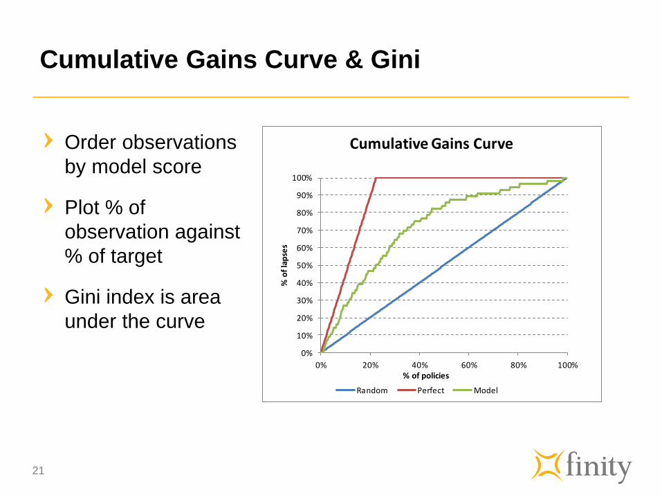
Cumulative Gains Curve & Gini

21

Order observations

by model score

Plot % of

observation against

% of target

Gini index is area

under the curve

0%

10%

20%

30%

40%

50%

60%

70%

80%

90%

100%

0% 20% 40% 60% 80% 100%

% o

f la

pse

s

% of policies

Cumulative Gains Curve

Random Perfect Model

ROC curve & Mann-Whitney U statistics

Order observations by

model score

Plot % of success

against % failure

Mann-Whitney U is

area under the curve

Can be expressed as

function of Gini and

rate of success

22

0%

10%

20%

30%

40%

50%

60%

70%

80%

90%

100%

0% 20% 40% 60% 80% 100%

ROC Curve

Are they any good for monitoring model

performance?

The measures are designed to compare the goodness of fit

of different models on the same data at the model building

stage

They work well when

the volume of the data is the same

The distribution of the response variable is the same

23

Monitoring issues for Deviance

24

𝐷𝑖 = −2 log 1 − 𝑝𝑖 𝑥 = 0

−2 log 𝑝𝑖 𝑥 = 1

For small P (0.05) Small (0.0511..)

Big (2.995..)

Deviance formula is sensitive to changes to the

scale/levels of the overall response

Consider separately:

Average predicted probability for cases which

were 0 (smaller is better)

Average predicted probability for cases which

were 1 (bigger is better)

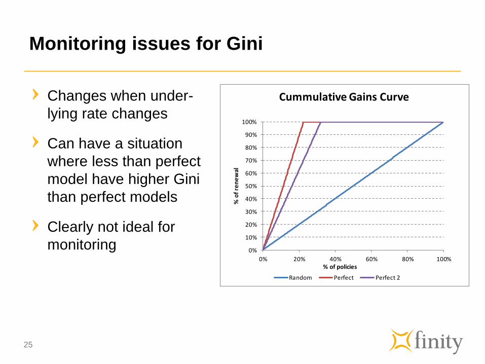
Monitoring issues for Gini

Changes when under-

lying rate changes

Can have a situation

where less than perfect

model have higher Gini

than perfect models

Clearly not ideal for

monitoring

25

0%

10%

20%

30%

40%

50%

60%

70%

80%

90%

100%

0% 20% 40% 60% 80% 100%

% o

f re

ne

wal

% of policies

Cummulative Gains Curve

Random Perfect Perfect 2

Adjustment for Gini

Adjust Gini by the ratio between

(A + B) and (A’ + B’)

B and (A + B)

Results much more consistent 26

0%

10%

20%

30%

40%

50%

60%

70%

80%

90%

100%

0% 20% 40% 60% 80% 100%

% o

f re

ne

wal

% of policies


0%

10%

20%

30%

40%

50%

60%

70%

80%

90%

100%

0% 20% 40% 60% 80% 100%

% o

f re

ne

wal

% of policies


A A’

B B’

Additional goodness of fit measures for model

monitoring – random partition A/E

Entire dataset is split into 100 random subsets and the

difference between actual and predicted measured

Error = ABS(Actual – Predicted) / Predicted. The exposure

weighted mean of this quantity is the measure of fit

27

Random Subset

Policy Count

Actual Rate

Predicted Rate Error

1 800 10% 10.5% 5%

2 850 10% 9.5% 5%

...

99 790 10% 11% 10%

100 830 10% 9.8% 2%

Total 80,000 10% 10% 5.5%

Determining tolerances

Not too hard for things like claim size, frequency etc. where

we have some ideas about their distribution either from

historical data or theoretical assumptions

For goodness-of-fit measures more difficult

One approach is to get some sense of volatility through

bootstrap samples

Also need to apply some common sense adjustments based

on what we are monitoring

28

• Standard model fit metrics not ideal for

monitoring

• Adjustments or alternative metrics

needed to account for changes in

volume and distribution

Case study

31

Model

Time Scale Chart Axes Min Max Unit

From Actual vs Expected 0% 100% 10%

To Gini 0% 100% 10%

Deviance 0% 100% 10%

Model Scorecard Decile 0% 100% 10%

Summary Actual and Expected

Value p-value Trend R2 p-valueGini 0.682 0.001 -0.23% 0.35 0.019Rand PartN A/E 0.112 0.042 -0.05% 0.06 0.786

CUMSUM p-value > average p-valueAvM > 1 67% 0.073 17% 0.019Gini Decr 58% 0.194 83% 0.003Rand Part A/E Incr 50% 0.387 100% 0.000

Exposure (total monitoring) 1,000,000Actual 20,000Rate 2.0%

Potential Impact Gini Monthly# Policies $M PremiumAvg Premium

Actual 1,000,000 500 500Model 1,100,000 500 500Ratio 0.909 1.000 1.100

Decile Graphs

Random Partition A vs E

Mis-Fitting VariablesVariable Name Scaled ∆ exposure % Levels >

v1 10.00 0.01 75%v2 9.10 0.01 11%v3 3.20 0.00 17%v4 2.30 0.00 25%v5 1.10 0.01 30%


Raw Prediction MAE Scaled Prediction MAE


Update

1 2 3 4 5 6 7 8 9 10

Actual Predicted Scaled Predicted

Auto Axes

Go To Data

Go To Data

Scenarios

32

• Gradual decrease in overall rate Scenario 1

• Sudden decrease in overall rate Scenario 2

• Behaviour change leading to new relativities, scale change Scenario 3

• Behaviour change leading to new relativities, no scale change Scenario 4

Model



To Gini 0% 100% 10%









Decile Graphs



v1 10.00 0.01 75%v2 9.10 0.01 11%v3 3.20 0.00 17%v4 2.30 0.00 25%v5 1.10 0.01 30%




Update

1 2 3 4 5 6 7 8 9 10


Auto Axes

Go To Data

Go To Data

Scenario 1 - Gradual decrease in overall rate

33

Actual and Expected



Model



To Gini 0% 100% 10%









Decile Graphs



v1 10.00 0.01 75%v2 9.10 0.01 11%v3 3.20 0.00 17%v4 2.30 0.00 25%v5 1.10 0.01 30%




Update

1 2 3 4 5 6 7 8 9 10


Auto Axes

Go To Data

Go To Data

Scenario 1 - Gradual decrease in overall rate

Trend identified after

6 months by

Cumsum and

random partition A/E

value

34

Summary

Value p-value Trend R2 p-valueGini 0.670 0.462 -0.09% 0.24 0.420Rand PartN A/E 0.210 0.073 0.33% 0.08 0.840


Model



To Gini 0% 100% 10%









Decile Graphs



v1 10.00 0.01 75%v2 9.10 0.01 11%v3 3.20 0.00 17%v4 2.30 0.00 25%v5 1.10 0.01 30%




Update

1 2 3 4 5 6 7 8 9 10


Auto Axes

Go To Data

Go To Data

Scenario 2 - Sudden decrease in overall rate

35

Actual and Expected



Model



To Gini 0% 100% 10%









Decile Graphs



v1 10.00 0.01 75%v2 9.10 0.01 11%v3 3.20 0.00 17%v4 2.30 0.00 25%v5 1.10 0.01 30%




Update

1 2 3 4 5 6 7 8 9 10


Auto Axes

Go To Data

Go To Data

Gini Monthly




Random partition A/E

increases but Gini

remains stable indicating

a change in scale but

not relativities

36

Model



To Gini 0% 100% 10%









Decile Graphs



v1 10.00 0.01 75%v2 9.10 0.01 11%v3 3.20 0.00 17%v4 2.30 0.00 25%v5 1.10 0.01 30%




Update

1 2 3 4 5 6 7 8 9 10


Auto Axes

Go To Data

Go To Data


37

Summary



Model



To Gini 0% 100% 10%









Decile Graphs



v1 10.00 0.01 75%v2 9.10 0.01 11%v3 3.20 0.00 17%v4 2.30 0.00 25%v5 1.10 0.01 30%




Update

1 2 3 4 5 6 7 8 9 10


Auto Axes

Go To Data

Go To Data

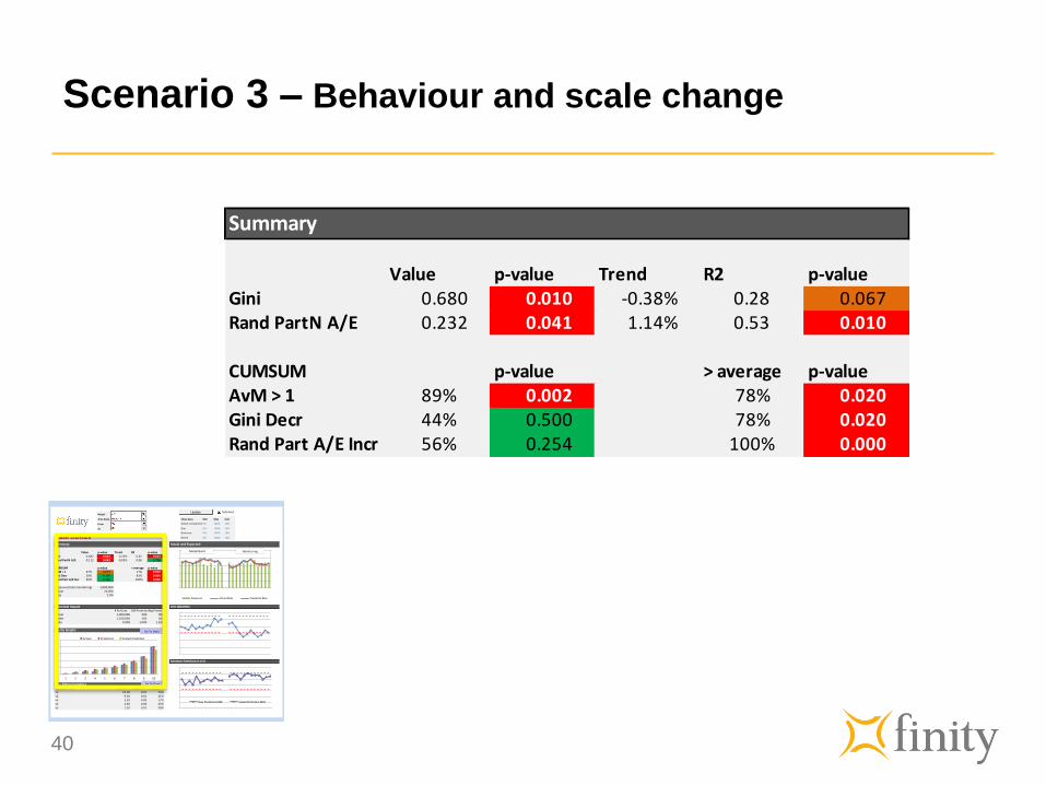
Scenario 3 – Behaviour and scale change

Behaviour change.

Relativities now

different to those

derived from model

data

38

Actual and Expected



Model



To Gini 0% 100% 10%









Decile Graphs



v1 10.00 0.01 75%v2 9.10 0.01 11%v3 3.20 0.00 17%v4 2.30 0.00 25%v5 1.10 0.01 30%




Update

1 2 3 4 5 6 7 8 9 10


Auto Axes

Go To Data

Go To Data


39

Gini Monthly



Model



To Gini 0% 100% 10%









Decile Graphs



v1 10.00 0.01 75%v2 9.10 0.01 11%v3 3.20 0.00 17%v4 2.30 0.00 25%v5 1.10 0.01 30%




Update

1 2 3 4 5 6 7 8 9 10


Auto Axes

Go To Data

Go To Data


40

Summary



Model



To Gini 0% 100% 10%









Decile Graphs



v1 10.00 0.01 75%v2 9.10 0.01 11%v3 3.20 0.00 17%v4 2.30 0.00 25%v5 1.10 0.01 30%




Update

1 2 3 4 5 6 7 8 9 10


Auto Axes

Go To Data

Go To Data

Scenario 4 – Change in behaviour but not scale

No change

discernable from

looking only at

overall actual vs

model

41

Actual and Expected



Model



To Gini 0% 100% 10%









Decile Graphs



v1 10.00 0.01 75%v2 9.10 0.01 11%v3 3.20 0.00 17%v4 2.30 0.00 25%v5 1.10 0.01 30%




Update

1 2 3 4 5 6 7 8 9 10


Auto Axes

Go To Data

Go To Data


Both Gini and

random partition A/E

indicate poor fitting

model

42

Gini Monthly



Model



To Gini 0% 100% 10%









Decile Graphs



v1 10.00 0.01 75%v2 9.10 0.01 11%v3 3.20 0.00 17%v4 2.30 0.00 25%v5 1.10 0.01 30%




Update

1 2 3 4 5 6 7 8 9 10


Auto Axes

Go To Data

Go To Data


43

Summary



Model



To Gini 0% 100% 10%









Decile Graphs



v1 10.00 0.01 75%v2 9.10 0.01 11%v3 3.20 0.00 17%v4 2.30 0.00 25%v5 1.10 0.01 30%




Update

1 2 3 4 5 6 7 8 9 10


Auto Axes

Go To Data

Go To Data


Variables affected

were: Vehicle

segment, State, Sum

insured, Vehicle Use

44


Vehicle Segment 47.32 0.03 100%State 15.34 0.01 83%sum insured 9.05 0.00 100%vehicle use 4.05 0.00 44%vehicle age 4.01 0.00 70%


Drilling down

45

Variable MisFit: State

Go To Main Dashboard

ACT NSW QLD SA TAS WA

Policies

Actual Rate

Predicted Rate

Update

Other issues

Other considerations

Do we need it if self adapting models (similar to the dynamic GLM that

was presented last year) are in place?

Most self adapting models automatically update parameter estimates as new

experiences becomes available

They often will not adapt with additional interactions or other model structure

changes are required

Model monitoring will still tell us whether the “self adapting” mechanism is

functioning

Seasonality – many types of models (e.g., claim frequency) will show

seasonal patterns which must be accounted for in the framework

Claim development

Economic conditions

47

• A monitoring framework needs a range of

metrics and statistical tests to be effective

• Combining multiple measures into a semi-

automated process enables efficient and

accurate monitoring

Questions?

49

Contact

John Yick

Principal

Tel: +61 2 8252 3384

www.finity.com.au

Michael McLean

Consultant

Tel: +61 2 8252 3315

www.finity.com.au

Distribution & Use

This presentation has been prepared for the

Finity Consulting Personal Lines Pricing &

Portfolio Management Seminar, held on 22

May 2014. It is not intended, nor

necessarily suitable, for any other purpose.

Third parties should recognise that the

furnishing of this presentation is not a

substitute for their own due diligence and

should place no reliance on this

presentation or the data contained herein

which would result in the creation of any

duty or liability by Finity to the third party.

Reliances & Limitations

Finity wishes it to be understood that the

information presented at the Seminar is of a

general nature and does not constitute

actuarial advice or investment advice.

While Finity has taken reasonable care in

compiling the information presented, Finity

does not warrant that the information

provided is relevant to a particular reader’s

situation, specific objectives or needs.

Finity does not have any responsibility to

any attendee at the conference or to any

other party arising from the content of this

presentation. Before acting on any

information provided by Finity in this

presentation, readers should consider their

own circumstances and their need for

advice on the subject – Finity would be

pleased to assist.

to freak out or to chill out? a guide to model monitoring · what is model monitoring? model...

Documents