To Editors, Journal of Graphics Tools:

We are submitting a major revision of Paper Number 300: ”Efficient Shadows ForSampled Environment Maps”, by Ben-Artzi, Ramamoorthi and Agrawala. We wouldlike to thank the reviewer for the thorough and careful reading of the paper. We havecompletely re-organized the text to address the comments made, and believe the paper ismuch clearer and more direct.

As for particular changes, we agree with (and thank) the reviewer, in that the pre-vious version was somewhat poorly organized, with a number of concepts discussed atvarious points in the paper, and some duplication resulting in a somewhat long manu-script. In the current version, the sections clearly separate out the concepts. Section 4discusses the framework components alone for estimating visibility and correcting thosepredictions. Section 5 compares both the accuracy and efficiency of various componentcombinations, clearly contrasting different possible choices and discussing which is better.Finally, Section 6 contains the entire discussion on optimizations, and implementation ofthe final optimized algorithm as well as time and memory considerations. We have alsosignificantly shortened the paper to make it more direct and readable. Below, we respondto specific points raised by the reviewer.

One important point these changes address is the reviewer comment regarding somesections duplicating each other. As suggested by the reviewer, the discussion of optimiza-tions is now in the final section 6 on implementation, rather than interspersed with themain discussion on framework components and their combination in sections 4 and 5.As suggested by the reviewer, we now focus section 4 on clearly laying out the idea andcomponents in the basic algorithm.

As regards the verboseness of the paper, we have paid heed to the comment of thereviewer regarding the very large captions on the figures in the original submission. Thecaptions have all been made shorter and clearer, with more of the descriptions movedto the text. We have also removed the line-by-line pseudocode description as suggested,making it much more succinct.

Another of the difficulties the reviewer mentioned was the insufficient discussion ofwarping vs not warping, where we described ”possibly warping” for much of the paper,and didn’t fully discuss the benefits and which we used. In the current version, this ismade much clearer. Warping vs not warping is presented as a fundamental frameworkcomponent rather than an optimization, in section 4.1.3 of the new manuscript. Thediscussion of benefits and disadvantages based on empirical testing is clearly describedand focused in section 5.3.1, where the recommendation to not warp, for greater efficiencyis also stated clearly.

The final point on presentation raised in the review concerns the mathematical termi-nology in the preliminaries section. While it is true that we do not use this later in thepaper, we believe it is important to make clear how the visibility sampling in this paperfits into the broader picture of computing the reflection equation. We now make thisexplicit in the paragraph, that should help in understanding the focus of our paper, andhow it would fit into a rendering algorithm.

We have also incorporated most of the other more minor comments that the reviewerhas made. For instance, we have moved the system specs to the text rather than captionin table 2, eliminated the duplicates of table 1, and for conciseness removed figure 5 inthe original version. We believe the figure placement is now also much more in line withthe text. Regarding our notation for GNU/GWB/SWB and so on, we now introduce thesymbols in section 4 while discussing each framework component, which should make thenotation clearer. In addition, we have reworked the figures and tables to accommodatethe JGT format.

Again, we would like to thank the reviewer for the time taken in reading our originalmanuscript, and for the very interesting additional comments for future work. We hopethat our manuscript will now be considered suitable for publication. Please let us know ifthere are any questions.

Yours sincerely,

The Authors

1

Efficient Shadows for Sampled Environment Maps

Aner Ben-Artzi Ravi Ramamoorthi Maneesh AgrawalaColumbia University Columbia University Microsoft Researchaner@cs.columbia.edu ravi@cs.columbia.edu maneesh@graphics.stanford.edu

Abstract

This paper addresses the problem of efficiently calculating shadows from environment maps

in the context of ray-tracing. Since accurate rendering of shadows from environment maps

requires hundreds of lights, the expensive computation is determining visibility from each pixel

to each light direction. We show that coherence in both spatial and angular domains can be used

to reduce the number of shadow-rays that need to be traced. Specifically, we use a coarse-to-

fine evaluation of the image, predicting visibility by reusing visibility calculations from 4 nearby

pixels that have already been evaluated. This simple method allows us to explicitly mark regions

of uncertainty in the prediction. By only tracing rays in these and neighboring directions, we

are able to reduce the number of shadow-rays traced by up to a factor of 20 while maintaining

error rates below 0.01%. For many scenes, our algorithm can add shadowing from hundreds of

lights at only twice the cost of rendering without shadows.

appr

oxim

atel

y eq

ual q

ualit

y

appr

oxim

atel

y eq

ual w

ork

60 million shadow rays standard ray-tracing

6 million shadow rays our method

7½ million shadow rays standard ray-tracing

Figure 1: A scene illuminated by a sampled environment map. The left image is rendered in POV-

Ray using shadow-ray tracing to determine light-source visibility for the 400 lights in the scene,

as sampled from the environment according to [Agarwal et al. 2003]. The center image uses our

Coherence-Based Sampling to render the same scene with a 90% reduction in shadow-rays traced.

The right image is again traced in POV Ray, but with a reduced sampling of the environment map (50

lights, again using [Agarwal et al. 2003]) to approximate the number of shadow-rays traced using our

method. Note that the lower sampling of the environment map in the right image does not faithfully

reproduce the soft shadows.

1 Introduction

Complex illumination adds realism to computer-generated scenes. Real-world objectshardly ever exist in environments that are well approximated by a small number of lights.We therefore focus on realistic shading and shadowing from environment maps, as firstdescribed by [Blinn and Newell 1976], and later by [Miller and Hoffman 1984], [Greene1986], and [Debevec 1998]. The subtle shadowing effects created by complex illuminationare one of the most important visual cues for realistic renderings. Correct shadowingrequires solving for the visibility of each light direction with respect to each pixel. Thisis extremely expensive, since the illumination can come from any direction in the envi-ronment map. We leverage recent sampling methods like [Agarwal et al. 2003], [Kolligand Keller 2003], and [Ostromoukhov et al. 2004], that reduce the environment to a fewhundred non-uniform directional lights. However, shadow testing for all sources at eachpixel is still the bottleneck in a conventional raytracer or other renderer.

In this paper, we show that the visibility function can be efficiently calculated by ex-ploiting coherence in both the angular and spatial dimensions. We recognize that theexpensive operation when lighting with complex illumination is the tracing of secondaryshadow-rays. Thus, we recommend tracing all primary eye-rays, and only culling shadow-rays, whenever possible. Our work is closest to that of [Agrawala et al. 2000], who exploitedcoherence in the visibility of an area light source to reduce the number of shadow-rayscast. We adapt their method to environment maps, and show that modifications to boththe spatial sharing and angular sharing of visibility information are required for accurateand efficient visibility sampling in the context of environment lighting. The salient differ-ences from area lighting are the lack of a well-defined boundary, lack of locality, and lackof efficient uniform sampling for environment lighting. By addressing all of these points,

2

we demonstrate, for the first time, how coherence-based visibility sampling can be usedfor full-sphere illumination.

We identify two important components of an algorithm estimating visibility by reusingpreviously calculated visibility, and explicitly tracing new shadow-rays to correct errors inthe estimate. By correctly sharing information among pixels, as well as light directions,we show that accurate visibility predictions can be achieved by tracing only about 10% ofthe shadow-rays that would normally be required by a standard raytracer without loss inaccuracy, as shown in Figure 1.

Contributions:

• We identify two components of a framework for exploiting coherence in the visibilityfunction (Section 4). We provide experience to aid the reader in assesing the ben-efits and drawbacks of possible alternatives and combinations for these components(Section 5).

• We present an optimized and simple algorithm that may be added to any ray-tracer toenable efficient compuation of shadows from sampled enviroment maps (Section 6.1).

• We provide pseudocode to assist implementation (Section 6.2), as well as online re-sources that include working code, data, animations, and scripts to recreate all imagesin this paper. (See www.cs.columbia.edu/cg/envmapshadows).

2 Previous Work

Previous works describe coherence-based methods for rendering scenes illuminated bypoint or area lights. Most of these techniques find image-space discontinuities and sharevisibility or shading information within regions bounded by discontinuities, thus reducingthe number of primary eye rays (and recursively, the number of shadow-rays). We discusssome of these methods below, and discover that image-space radiance interpolation is notwell-suited for complex illumination. Furthermore, an efficient method cannot rely on thepresence of a light boundary, the locality of the light(s), nor the ability to uniformly samplethe lighting. When these assumptions are broken, existing methods often degenerate toan exhaustive raytracing for both eye- and shadow-rays.

[Guo 1998] was able to efficiently render a scene lit by area light sources by findingradiance discontinuities in image-space. A sparse grid of primary rays was fully evaluated,and radiance discontinuities were discovered by comparing the results of these calculations.The rest of the image pixels are bilinearly interpolated, thus culling the actual primary andsecondary rays for those pixels. Unlike area light sources, environment map illuminationproduces continuous gradients instead of discoverable discontinuities. The method usedby [Guo 1998] would incorrectly interpolate large regions of the scene that in fact havesmooth, yet complex variations in radiance.

[Bala et al. 2003] also interpolate radiance in image-space, but determine the regionsof interpolation by examining the visibility of lights. Each pixel is classified as empty,simple, or complex, depending on whether it contains 0, 1, or more discontinuities of lightvisibility. Only complex pixels are fully evaluated. When rendering images illuminatedby a sampled environment map, nearly every pixel becomes complex. This is due to thepresence of hundereds of light sources, several of which exhibit a change in visibility whenmoving from one pixel to the next.

[Hart et al. 1999] demonstrated an analytic integration method for calculating irradiancedue to area light sources. They find all light-blocker pairs, exploiting coherence of thesepairings between nearby pixels. The lights are then clipped against the blocker(s) toproduce an emissive polygon corresponding to the visible section of the light source. Thelight-blocker pairs are discovered using uniform sampling of the solid angle subtended bythe area light source, taking advantage of the light’s locality. For an environment mapwhich subtends the entire sphere of directions, this method degenerates to brute-forcevisibility sampling.

[Agrawala et al. 2000] achieve their speedup by assuming that visibility of the lightsource is similar for adjacent pixels. They determine visibility of regularly spaced samplesof the area light source, and then share that visibility information with the subsequentpixel of the scanline order. Errors are corrected by explicitly tracing new shadow-raysto light samples that lie along visibility boundaries (and recursively flooding the shadowtraces when errors are detected). Locality of the area light source and a well-defined edgeensured that the number of samples was small, and boundaries were well-defined.

Our work also relates to much recent effort on real-time rendering of static scenesilluminated by environment maps. Precomputed radiance transfer methods such as [Nget al. 2003] and [Sloan et al. 2002] have a different goal of compactly representing andreusing the results of exhaustive calculations. They perform a lengthy precomputation

3

A

B

Figure 2: The environment map for Grace Cathedral (left) is sampled into 82 directional lights. Each

light is surrounded by the directions nearest to it, as defined by the Voronoi diagram (right). Note

that the sampling is irregular, with region A being densely sampled and region B containing sparse

samples.

step during which standard raytracing is used to compute the radiance transferred to allparts of a static scene. In contrast, we focus on computing the visibility of an arbitraryscene more efficiently. PRT methods may benefit from using our algorithm in the raytracerthey employ for the precomputation stage.

3 Preliminaries

In this section, we briefly desctibe how our work relates to rendering engines that solvethe reflection equation. The exit radiance at a point, x, in the direction ω, is given by

L(x, ω0) =

∫Ω2π

fr(ω,ω0)L(ω)V (x, ω)(ω · n)dω,

where x is a location in the scene with a BRDF of fr, n is the normal, and ω is a directionin the upper hemisphere, Ω2π . V (x, ω) is the 4D, binary visibility function of the scene.The light-space of each location, xi, is the set of directions in the upper hemisphere, Ω2π ,centered at xi. V (xi, ω) assigns to each direction in the light-space of xi, a binary valueindicating whether occluding geometry exists in that direction, or not. [Agarwal et al.2003] demonstrated that the integral above can be turned into an explicit sum over a setof well-chosen directions ωi, with associated regions or cells, as shown in Figure 2 right.An efficient approximation of several hundred directional lights can be found for mostenvironment maps, and we assume that such a technique has been used. Often, thehardest part of solving for L(x, ω0) is computing the visibility term, V (x, ω). Our workconcentrates on making this visibility calculation more efficient. Any system which cansubstitute its computation of V (x, ω) in the above equation can make use of the methodsdescribed in this paper. We demonstrate that a sparse set of samples in x×ω can beused to reconstruct V (x, ω) with a high degree of accuracy.

Given a set of directional lights, we partition the set of all directions into regions thatare identified with each light, as seen in Figure 2 right. This is done by uniformly samplinga unit disk and projecting each sample onto the unit sphere to obtain a direction. Thesample is then assigned the ID (visualized as a color) of the light that is closest to theobtained direction, thus constructing the Voronoi diagram. To improve the resolution ofregions near the edge of the disk, a transformation such as parabolic mapping ([Heidrichand Seidel 1998]) should be used. In our experience, even for environment maps sampledat 400 lights, with the smallest cells near the horizon, a 513×513 pixel Voronoi diagramsuffices. (As presented here, only directions where y > 0 appear in the diagram. Theextension to the full sphere with a second map is straightforward.) We will see that anotion of adjacency in the light-space is needed. Since the lights are not evenly spaced, weidentify all the neighbors of a light region by searching the Voronoi diagram. We foundthat the average connectivity of lights in our sampled environments is 6. Because we areusing environment maps that represent distant light sources, the Voronoi diagram, andthe list of neighbors for each light cell is precomputed once for a particular environment.

4 Framework Components

Leveraging coherence to estimate visibility occurs in two phases. First, we construct anapproximate notion of visibility based on previous calculations (Section 4.1). Then wemust clean up this estimate by identifying and correcting regions that may have beenpredicted incorrectly (Section 4.2). For the rest of the discussion we will refer to a pixel,and the scene location intersected by an eye-ray through that pixel, interchangeably.

4

Figure 3: Grid-Based Evaluation. First, the image is fully evaluated at regular intervals. This

produces a coarse grid (left). Next, the center (blue) of every 4 pixels is evaluated based on its

surrounding 4 neighbors (gray). All 4 are equidistant from their respective finer-gird-level pixel

(center). Again, a pixel is evaluated at the center of 4 previously evaluated pixels (right). At the end

of this step, the image has been regularly sampled at a finer spaceing. This becomes the new coarse

level, and the process repeats.

4.1 Estimating Visibility

Our goal is to reuse the points of geometry that represent intersections between shadow-rays and objects in the scene. To predict the visibility at one spatial location, we considerthe occluding geometry discovered while calculating visibility at nearby locations, thustaking advantage of spatial coherence. We must choose which previously evaluated pixelswill be most helpful when attempting to reuse visibility information. We explore theoptions of scanline and grid-based pixel evaluations.

4.1.1 Scanline Ordering (S)When evaluating the pixels in scanline order, we use the previous pixel on the scanline, aswell as the two pixels directly above them, on the previous scanline. The reasoning behindthis is that visibility changes very little from pixel to pixel, and thus using the immediateneighbors gives a good first approximation to the visibility at the current pixel.

4.1.2 Grid-based Ordering (G)Scanline ordering has the notable limitation that all of the previously evaluated pixelscome from the same general direction (up, and to the left). Therefore, we present analternative which always allows us to reuse visibility from 4 previously evaluated pixelseach one from a different direction. In this case, the pixel location for which visibility isbeing evaluated is the average of the pixels that are informing the estimation process. Toa first approximation, the visibility can also be taken to be the average of the visibilityat the 4 nearby pixels. This is similar to the coarse-to-fine subdivision first introduced by[Whitted 1980] for anti-aliasing. The precise pattern (detailed in Figure 3) is chosen hereto maximize reuse of information from already-evaluated pixels. We have found that aninitial grid spacing between 32 and 8 pixels generally works well for minimal overhead.

4.1.3 Warping (W) and Not Warping (N)When blockers are distant, the visibility of a light source at a given pixel can be assumedto be the same at a nearby pixel. However, when blockers are close to the surface beingshaded, it may be advantageous to warp the direction of a blocker in the nearby pixel’slight-space, to a new location in the light-space of the pixel being shaded, as in Figure 4.

Though mathematically correct, warping does not produce a completely accurate re-construction of blocked regions. As in any image-based rendering (IBR) scheme, warpingresults in holes, and other geometry reconstruction errors. Estimation errors must becorrected, as described in the next section. We have discovered through empirical testingthat this correction method can work well both when warping, and when not warpingthe blockers from nearby pixels. In both cases, the initial visibility estimation containsenough accurate information to allow for good error correction.

x1 x2

a b a b

x 's light-space1 x 's light-space2

a b

Figure 4: Warping Blockers. Visibility for x1 is computed by tracing shadow-rays and finding a

and b. The visibility for x2 is predicted by warping blocker points a and b to their positions in the

light-space relative to x2 .

5

Path A: Boundary Flooding

A2A3 B3

1

B2

Path B: Uncertainty Flooding

Figure 5: 1: The blockers (black dots) from 3 neighboring pixels (not shown) are placed in the

light-space of the current pixel. Each hexagonal cell represents a cell in the Voronoi diagram that

partitions the light-space. Path A. A2: Light cells which contain more blockers than the threshold

(1) are predicted as blocked (grey), while others are predicted as visible (white). A3: Light cells whose

neighbors’ visibility differs are shadow-traced (blue center). Path B. B2. Light cells that contain

many (in this case 3 since we are using 3 previous pixels) blockers are predicted as blocked. Those

that contain no blockers are predicted as visible. Light cells containg few (1 or 2) blockers are marked

as uncertain and shadow-traced (blue center). B3. The neighboring light cells of all uncertain cells

are shadow-traced.

4.1.4 Constructing the Visibility EstimateThe visibility estimate for a pixel is constructed as follows: Each pixel is informed ofblockers that were discovered in its neighbors (scanline or grid-based). The direction tothese blockers is known, and may be warped to adjust for disparity between the pixel andits informers. At this point the pixel is aware of as many blockers as existed in all ofits neighbors, combined. Each blocker is assigned to one of the cells in the light-space ofthat pixel. (By using the precomputed Voronoi diagram discussed in Section 3, findingthe cell corresponding to any direction is a simple table lookup.) Some cells receive manyblockers, some few, while others may receive none, as seen in Figure 5.1. The followingsubsection discusses how to interpret and correct this data.

4.2 Correcting Visibility Estimates

We have shown that spatial visibility coherence among nearby pixels can be used to makeeducated estimates of visibility. In this section we discuss how angular coherence amongnearby directions can be used to correct errors produced by the estimation phase. Oncesome estimate of visibility exists for the light-space of a pixel, we would like to identifyregions of the light-space that may have been estimated incorrectly, and fix them.

4.2.1 Boundary Flooding (B)Any cell that contains more blockers than a given threshold is assumed to be blocked(Figure 5.A2). Our experience shows that the exact value of this threshold has little effecton the final algorithm, and we set it to 0.99. This estimation of visibility is prone to errornear the boundary of cells which are visible, and cells which are blocked. This is becausesuch a boundary is likely to exist, but may not lie exactly where the estimate has placed it.We attempt to correct these errors by explicitly casting shadow-rays in the directions thatlie along a boundary (Figure 5.A3). Wherever the shadow-ray indicates that an error hadbeen made in the estimation stage, we recursively shadow trace all the adjacent regions.This process continues until all shadow-rays report back in agreement with the estimate.

4.2.2 Uncertainty Flooding (U)Instead of guessing that boundaries are prone to error, we can use a more explicit measureof when we are uncertain of the visibility constructed by the estimation phase. Cells thatcontain many (4 in grid-based, 3 in scanline) blockers are considered blocked because allof the informing pixels agree that it is blocked. Similarly, cells without any blockers areconsidered visible. Whenever the neighbor pixels disagree on the visibility for any cellof the light-space (indicated by a small number of blockers), we mark it as uncertain(Figure 5.B2). We explicitly trace shadow-rays for these regions, and flood outwards,recursively tracing more shadow-rays when the estimation disagrees with the shadow-ray(Figure 5.B3).

5 Analyzing Possible Component Combinations

So far, we have developed four variations of the first phase: estimating visibility. Wecan use scanline evaluation (S) or grid-based evaluation (G), and for each of these, wemay choose to warp (W) or not warp (N) the blockers from nearby pixels. We havealso developed two variations for the second phase: correcting the estimate. We can

6

TRUE our method (OPT)TRUE our method (OPT)

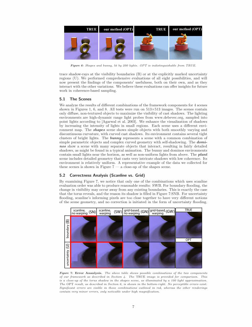
Figure 6: Shapes and bunny, lit by 200 lights. OPT is indistinguishable from TRUE.

trace shadow-rays at the visibility boundaries (B) or at the explicitly marked uncertaintyregions (U). We performed comprehensive evaluations of all eight possibilities, and willnow present the findings of the components’ usefulness, both on their own, and as theyinteract with the other variations. We believe these evaluations can offer insights for futurework in coherence-based sampling.

5.1 The Scenes

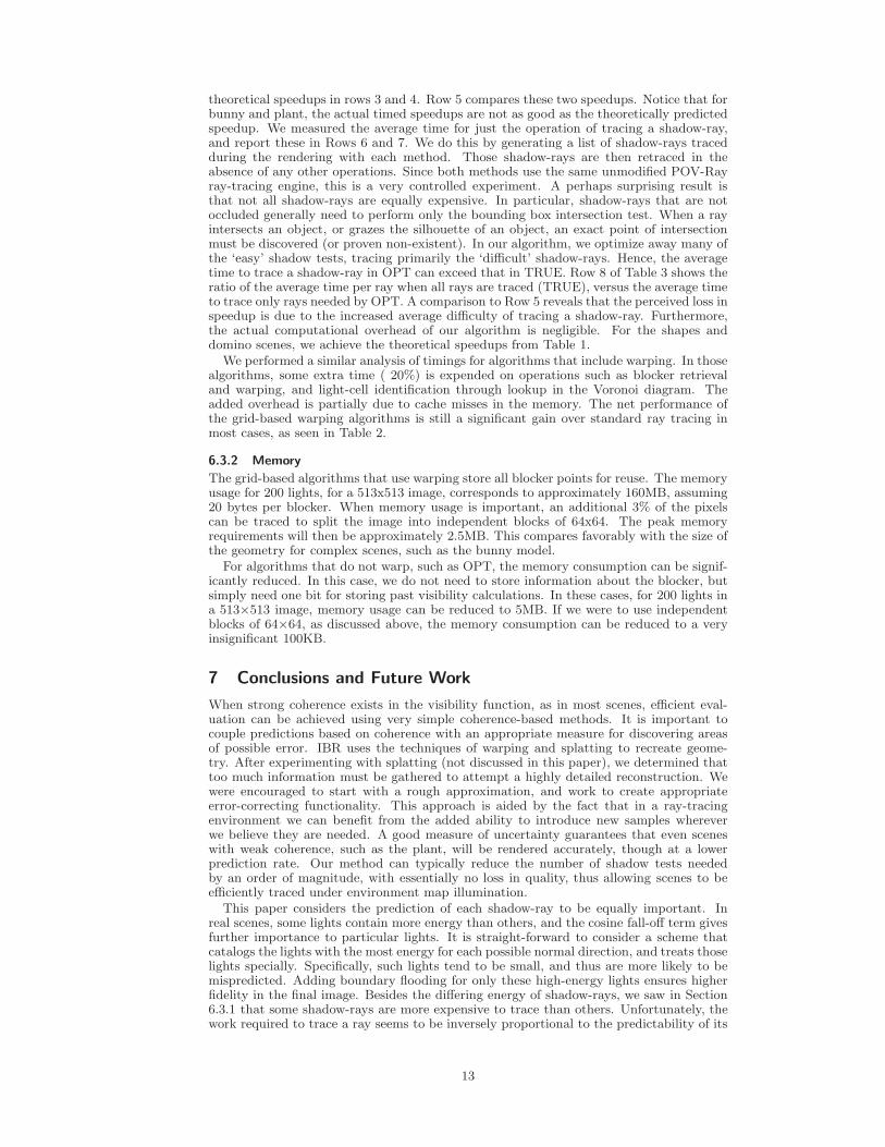
We analyze the results of different combinations of the framework components for 4 scenesshown in Figures 1, 6, and 8. All tests were run on 513×513 images. The scenes containonly diffuse, non-textured objects to maximize the visibility of cast shadows. The lightingenvironments are high-dynamic range light probes from www.debevec.org, sampled intopoint lights according to [Agarwal et al. 2003]. We enhance the visualization of shadowsby increasing the intensity of lights in small regions. Each scene uses a different envi-ronment map. The shapes scene shows simple objects with both smoothly varying anddiscontinuous curvature, with curved cast shadows. Its environment contains several tightclusters of bright lights. The bunny represents a scene with a common combination ofsimple parametric objects and complex curved geometry with self-shadowing. The domi-nos show a scene with many separate objects that interact, resulting in fairly detailedshadows, as might be found in a typical animation. The bunny and dominos environmentscontain small lights near the horizon, as well as non-uniform lights from above. The plantscene includes detailed geometry that casts very intricate shadows with low coherence. Itsenvironment is relatively uniform. A representative example of the data we collected forthese scenes is shown in Figure 7 — a close-up of the shapes scene.

5.2 Correctness Analysis (Scanline vs. Grid)

By examining Figure 7, we notice that only one of the combinations which uses scanlineevaluation order was able to produce reasonable results: SWB. For boundary flooding, thechange in visibility may occur away from any existing boundaries. This is exactly the casethat the torus reveals, and the reason its shadow is filled in Figure 7:SNB. For uncertaintyflooding, scanline’s informing pixels are too close together to have very different notionsof the scene geometry, and no correction is initiated in the form of uncertainty flooding.

scanline, no warping

scanline, warping

grid-based,no warping

grid-based,warping(SN) (SW) (GN) (GW)

un

cert

ain

tyb

ou

nd

ary

(U)

(B)

TRUE

OPT

Figure 7: Error Ananlysis. The above table shows possible combinations of the two components

of our framework as described in Section 4. The TRUE image is provided for comparison. This

is a close-up of the torus shadow in the shapes scene, as illuminated by a 100 light approximation.

The OPT result, as described in Section 6, is shown in the bottom-right. No perceptible errors exist.

Significant errors are visible in those combinations outlined in red, whereas the other renderings

contain very minor errors, only noticable under high magnification.

7

shapes bunny plant dominos

21

lights:TRUESWBGWBGNBGWUGNUOPT

5010040.522.021.710.49.44.8

10010034.317.917.110.78.84.6

20010026.315.113.811.08.34.5

40010022.412.410.611.37.54.3

5010052.4

.521.29.18.14.6

10010042.616.615.89.47.74.4

20010033.613.512.010.27.24.1

40010025.911.69.3

11.56.73.9

5010063.237.837.733.335.321.4

10010051.634.534.632.433.820.9

20010044.332.632.732.333.420.8

40010039.730.530.631.131.920.2

5010054.531.630.320.417.39.4

10010043.628.225.722.316.99.2

20010036.024.921.922.216.39.1

40010028.821.818.022.615.38.8

Table 1: Percentage of Shadow-Rays Traced. The entries for the table indicate the percentage of

shadow-rays where N · L > 0 that were traced by each method. For each scene an environment map

was chosen, and then sampled as approximately 50, 100, 200, and 400 lights.

shapes bunny plant dominosec speedup sec speedup sec speedup sec speedup

primary rays only (EYE) 4.0 N/A 4.0 N/A 4.4 N/A 4.2 N/Aground truth (TRUE) 75.3 1.0 80.8 1.0 152.3 1.0 124.9 1.0scanline, warping, boundary (SWB) 34.9 2.2 54.8 1.5 120.3 1.3 67.1 1.9grid-based, warping, boundary (GWB) 25.2 3.0 36.7 2.2 113.2 1.3 55.7 2.2grid-based, no warping, boundary (GNB) 16.8 4.5 23.2 3.5 95.1 1.6 35.4 3.5grid-based, warping, uncertainty (GWU) 19.6 3.8 30.6 2.6 109.0 1.3 47.1 2.6grid-based, no warping, uncertainty (GNU) 11.2 6.7 16.7 4.8 94.7 1.6 23.8 5.2optimized algorithm (OPT) 7.1 10.5 10.7 7.6 58.3 2.6 14.7 8.5

environments sampled at 200 lights

Table 2: Timings. The wall-clock timings for the full rendering with 200 lights, shown here, are

related to, but not equivalent to the reduction in work as measured in shadow-rays traced (see Table 1).

Hence, there can be staircasing artifacts as seen in Figure 7:SNU. Even with warping,uncertainty flooding from the three pixels immediately to the left and above does notsuffice, although it performs somewhat better, as seen in Figure 7:SWU. Thus, we mustuse warping and boundary flooding in scanline algorithms. It is interesting to note thatthis corresponds closely to the approach of [Agrawala et al. 2000].

All four grid-based possibilities (Figure 7:G--) give almost error-free results. The coarse-to-fine nature of grid-based evaluation is robust in the presence of different scales ofvisibility events. In addition, by using the grid-based approach, boundary and uncertaintyregions are marked conservatively enough to allow the correction stage to fix nearly allthe errors of the estimate. The details of each case are discussed in the next subsection.

5.3 Performance Analysis

The previous subsection concluded that three of the scanline algorithms are error-prone(outlined in red in Figure 7), and we do not consider them further. We now examinethe efficiency of each of the remaining combinations (SWB, GWB, GWU, GNB, GNU).Tables 1 and 2 compare the performance for each of the four scenes. Table 1 reports thepercentage of shadow-rays traced for each method, at different light sampling resolutionsof the scenes’ environments (50, 100, 200, 400). Table 2 shows the actual running timesfor rendering each scene with 200 lights, as timed on an Intel Xeon 3.06GHz computer,running Windows XP. The times reported in Table 2 include the (relatively small) timefor the initial setup of the raytracer and tracing just the EYE rays for each pixel, as wellas performing the diffuse shading calculation. The errors in the five remaining algorithmsare generally small (<0.1%) either when measured as absolute mispredictions, or whenviewed as the resulting color shift in the image. All of these algorithms enable significantreductions in the number of shadow-rays traced, with negligible loss in quality.

5.3.1 To Warp or Not to WarpThe motivation for warping blockers into the local frame of a pixel is that it may producea better approximation of the occluding scene geometry. This turns out to be counterpro-ductive for non-uniformly distributed samples of the light-space. Consider Figure 2 right .When the blockers in an area of densely sampled lights (region A), are warped onto anarea of sparse lights (region B), large cells in region B that are mostly visible may receivea large number of blockers, clustered in a corner of the cell. These would be incorrectlyestimated as blocked. Symmetrically, if warping occurs form a sparse region to a denseone, cells that are actually blocked may not receive any blockers and be erroneously es-timated as visible. When the spacing of the light samples is not uniform, warping can

8

introduce more errors in the visibility estimation, requiring more work to be done in thecorrection phase.

When comparing GWU with GNU and GWB with GNB, Table 1 shows that the non-warping algorithms perform slightly better for all but the plant scene. When comparingthe warping algorithms (GWB, GWU) to the equivalent non-warping algorithms (GNB,GNU) in Table 2, we can see a significant speedup in the wall-clock timings. Not warpingrequires fewer instructions since a simple count of the blockers in each cell suffices, whereaswarping must perform the 3D transformation of the blockers and project them into thenew cells. One additional advantage of not warping is that we eliminate the dependence onaccurate depth information for the blockers. This can be useful when rendering enginesoptimize the intersection test of shadow-rays by stopping as soon as an intersection isfound, without discovering the true depth of the closest blocker. (To obtain controlledcomparisions, we did not turn on this optimization.)

5.3.2 Boundary Flooding vs. Uncertainty FloodingSince the illumination from an environment map spans the entire sphere, many visibilityboundaries can exist, resulting in flooding to most of the lights when boundary floodingis used. Uncertainty flooding has the advantage of being restricted to those areas whichare visible at some neighboring pixels, and blocked at others. It is particularly well suitedto combat the sampling discrepancies described in the previous subsection (see Section5.3.1 and Figure 2). When under- or over-sampling of the light-space occurs, some cells inthat region receive few (1-3) blockers, and trigger explicit shadow traces for their neigh-bors. Marking cells as uncertain is equivalent to finding image-space discontinuities forindividual shadows. If such a discontinuity passes through the area surrounded by theinforming pixels, that light is marked as uncertain in the current pixel. In essence, uncer-tainty flooding concentrates on regions with image-space discontinuities, while boundaryflooding concentrates on light-space discontinuities.

Looking at Table 1, we see that in all cases, uncertainty flooding performs about twiceas well as the corresponding boundary flooding algorithm, at the lower resolutions. Inparticular, the first row (shapes50), shows GWB doing 22% of the work and GWU doingonly 10%. Similarly, GNB does 22% of the work, while GNU does only 9%. This indicatesthat marking boundaries as regions that require shadow-tracing is an overly-conservativeestimate. In our experience, not all visibility boundaries are error-prone.

Since the work done by boundary flooding is proportional to the area of the light-spaceoccupied by boundaries, its performance is strongly dependent on the sampling rate of theenvironment. Notice that for shapes, bunny, and dominos, boundary flooding algorithmsdegrade by a factor of 2 as the light resolution is decreased from 400 to 50. On theother hand, the performance of algorithms based on uncertainty flooding is relativelyindependent of the number of lights.

5.4 Discussion of Analysis

The examples shown in Figure 7 indicate that scanline evaluation order is much moreconstrained than grid-based. This is primarily because the small increments as the scanlineprogresses are sensitive to the scale of changes that may occur in visibility. We see in theresults outlined in red in Figure 7, that a missed visibility event propagates along thescanline until some other event triggers its correction via flooding. It is instructive tocompare GWB and SWB in Table 1, and notice that GWB is more efficient by about afactor of 2 for most cases. One reason for this is that scanline must consider the lights nearthe horizon as part of a boundary. New blockers that rise over the horizon as the scanlineprogresses are missed without flooding on the lights near the horizon of the pixel’s localframe. On the other hand, grid-based evaluation incorporates information from all fourdirections. This enables it to mark new visibility events as regions of uncertainty whenthey occur between the 4 informing pixels (i.e. near the pixel of interest).

Correctness is achieved when the correction phase is given an accurate guess of whereerrors might exist in the initial estimate. Efficiency is achieved when the original estimateis good, and indicators of possible error are not overly-conservative. For the algorithmsthat correctly combine the estimation and correction phases, accuracy is always obtained.In difficult scenes that exhibit low coherence (such as the plant), the algorithms degradein performance, but still produce accurate results.

6 Optimizations and Implementation

Based on the analysis of the previous section, we determine that GNU is the best combina-tion of the framework components for both accuracy and performance. We also renderedanimations for all of our test scenes by rotating the environment to see if any popping

9

TRUE

TRUE OPT

OPT

GNU FLO-OPT

Figure 8: Plant. The plant image, seen here as illuminated by a 100 light approximation of the

Kitchen environment, has very detailed shadows with low coherence. Nevertheless, our algorithms

produce a very accurate image, as seen in the direct comparisons and closeups.

artifacts would occur. All of the animations using GNU were indistinguishable form theTRUE animation. We therefore base our optimized algorithm (OPT) on GNU, makingit grid-based, without warping, and using uncertainty flooding as the means of correctingerrors (Section 6.1). We describe the implementation details for adding a GNU-basedalgorithm to any standard ray-tracing system in Section 6.2. Finally, we take an in-depthlook at the time and memory usage implications of these methods (Section 6.3).

6.1 Optimized Algorithm

More than half of the shadow-rays traced by our algorithms are triggered by flooding. Wehave seen that both boundary and uncertainty flooding are effective methods for correctingprediction errors. A close inspection of the shadow-rays traced due to flooding reveals thatmany of them agree with the original visibility estimate, and therefore only serve to haltfurther flooding, without contributing anything to the visibility calculation. We can avoidmany such shadow-traces by combining the ideas of uncertainty and boundary flooding.We still shadow-trace all regions of uncertainty as indicated by the original visibilityestimate (Figure 5.A2). However, instead of flooding to all neighbors (typically 6) of acell whose shadow-trace disagrees with the estimate, we only flood to those neighboringcells that also disagree with the shadow-trace result. This means that for uncertaintyregions that lie on a border, we only flood onto one side of the border; trying to findwhere it truly lies. This optimization reduces the number of flood-triggered traces byabout 40%. For complex shadows, small artifacts are introduced by this method, asmay be visible in the Figure 8:OPT close-up, but we feel that the performance gain isworth the slight difference in image quality. Since animations are more sensitive to smalldifferences, we recommend that this optimization only be used for stills, and omitted inanimations. (A comparison of these animations for the shapes scene is available online atwww.cs.columbia.edu/cg/envmapshadows/)

In an effort to further reduce the number of shadow-rays traced due to flooding, we notethat half of the image pixels are contained in the finest grid — when the initial estimateis informed by a pixel’s immediate neighbors. If all 4 neighbors agree on the visibility of aparticular light, the center pixel can only disagree if there is a shadow discontinuity smallerthan a single pixel passing through it. Since the image cannot resolve elements smallerthan a single pixel, we ignore these sub-pixel shadow discontinuities and turn off floodingaltogether at the grid’s finest level only (FLO). We still rely on error correction due toexplicit uncertainty marking. This reduces the total number of shadow-rays required tocalculate the image by about 25%, without adding any noticeable artifacts to the finalimage, as seen in the Figure 8:FLO-OPT close-up. This optimization also is safe foranimations, as its effects are only noticeable at a sub-pixel level. Sub-pixel sampling forantialiasing is a popular method employed by many rendering engines. When such a

10

feature is used in conjunction with our method, the highest resolution of sampling shouldbe considered to be the native image resolution for the purposes of defining the grid.

Our optimized algorithm (OPT) uses the above two methods of restricting flooding;flooding only to neighbors that disagree with the shadow-ray, and not flooding at the finestgrid level. The high quality of OPT can be seen in Figures 1, 7, 6, and 8. The close-upsin Figure 7 and Figure 8 reveal that OPT produces images nearly indistinguishable fromthe ground-truth (TRUE). Even on the stress-test provided by the plant scene (Figure 8),OPT has only a 0.4% error rate, as measured in actual shadow-ray prediction errors. Theerror rate for OPT on the bunny is 0.0026%, meaning only 1 in 38,000 shadow-rays disagreefrom ground-truth. In terms of visual quality of the images OPT produces accurate resultsfor all the scenes. As visualized in the final images, these errors produce rendering that arenearly identical to the true images when viewed as standard 24 bit RGB images. Addingthe above two optimizations typically leads to a 50% reduction in the number of shadow-rays traces, when compared to GNU. As reported in Table 1, this can result in a factorof 20 improvement in efficiency over standard visibility testing in ray-tracers. In Table 2,the timings show that as OPT’s performance improves, shadow-tracing is no longer thebottleneck for rendering. In the shapes scene, tracing the primary eye rays (4.0 seconds)takes longer than adding complex shadows to the scene (3.1 seconds).

6.2 Implementation

procedure Calculate-All-Visibilities()1 for (gridsize = 16; gridsize > 1; gridsize /= 2) do2 foreach pixel, p, in current grid do3 lights-to-trace ← ∅;4 n[1..4] ← Find-Evaluated-Neighbors(p);5 object(p) ← Trace-Primary-Ray-At-Pixel(p);6 if object(n[1]) == object(n[2]) == object(n[3]) ==

object(n[4]) == object(p) then7 foreach light, L, in sampled-environment-map do8 if vis(n[1], L) == vis(n[2], L) ==

vis(n[3], L) == vis(n[4], L) then9 vis(p, L) ← vis[n[1], L);

else10 vis(p, L) ← ‘uncertain’;11 lights-to-trace ← lights-to-trace ∪ L;

endifendforeach

12 Flood-Uncertainty(p);else

13 foreach light, L, in sampled-environment-map do14 vis(p, L) ← Trace-Shadow-Ray(p, L);

endforeachendif

endforeachendfor

Our algorithms are all very simple to add to a conventional ray-tracer or other renderingsystem. We have done so in the context of a widely available ray tracer, POV-Ray. Addingcoherence-based sampling requires few changes to the core rendering engine, and uses onlya few additional simple data structures for support. Furthermore, in our experience, careneed not be taken to ensure that the implementation is engineered precisely. Even ifit does not adhere strictly to our method, it will still provide a vast improvement overfull ray-tracing. In particular, GNU and OPT are very simple to implement. For eachpixel, once the 4 nearby pixels are identified in the grid-based evaluation, a simple checkof agreement for each light is performed. If all 4 pixels agree that a light is blocked orvisible, it is predicted as blocked or visible, respectively. When the 4 pixels do not agree ona particular light, it is shadow-traced, with possible flooding to neighboring lights. If theoptimizations are used, only neighbors whose prediction disagrees with the shadow-traceare traced, and no flooding to neighbors is performed at the final grid level. Code forGNU is shown in procedure Calculate-All-Visibilities.

Lines 1–4 describe the use of grid-based evaluation as shown in Figure 3. To primethis process, the coarsest level of the grid is evaluated at a scale of 16 pixels, which wefound to be suitable for all of the scenes we tested. For each of these pixels (<0.5% of the

11

image), all shadow-rays are traced. This is comparable to the priming for scanline whichrequires the top row and left column to be fully evaluated ( 0.4% for 513x513 images).In lines 5 and 6, we perform a sanity check to make sure that only visibility calculationsrelating to the same scene object are used for estimation. We have found that there is asignificant loss in coherence when the informing pixels are not on the same object as thecurrent pixel. We therefore fully shadow-trace around these silhouette edges to determinevisibility. For very complex scenes such as the plant in Figure 8, explicitly tracing in thissituation traces 7% of the shadow-rays. For average scenes like those in Figure 1 andFigure 6, this results in about 1–3% of the shadow-rays.

procedure Flood-Uncertainty(pixel p)1 while (lights-to-trace ∩ set-of-untraced-lights(p)) = ∅,

with an L from the above intersection do2 tempVis ← Trace-Shadow-Ray(p, L);3 if tempVis = vis(p, L) then4 vis(p, L) ← tempVis;5 foreach of L’s neighbors, N do6 lights-to-trace ← lights-to-trace ∪ N

endforeachendif

endwhile

In lines 7–11, the initial rough estimate of visibility is formed as shown in Figure 5 steps1 and A2. In line 12, the error correction phase is called, as described in Section 4.2.2, anddiagrammed in Figure 5.A3. The pseudocode for this is shown in Flood-Uncertainty.

When Flood-Uncertainty is called, the set lights-to-trace contains all those lights whichwere deemed ‘uncertain’. None of these have been traced yet. All other lights have hadtheir visibility predicted, but also were not explicitly traced. Line 1 checks to see if thereare any lights in lights-to-trace which have not yet been shadow-traced. If any such light,L, is found, a shadow-ray is traced from the object intersection for p in the direction ofL, at Line 2. At Line 5, the neighbors of L are added to the list of lights to trace. IfOPT were being implemented, line 5 would only add those neighbors whose predictiondisagreed with tempVis. It may seem reasonable to remove a light from lights-to-traceonce it has been traced, rather than checking against all the untraced lights in Line 1.However, doing so would lead to an infinite loop since Line 6 would add a neighbor, andwhen that neighbor got traced, it would add the original light.

6.3 Time and Memory Considerations

In this section, we evaluate some of the more subtle (yet interesting) aspects of coherence-based visibility sampling.

6.3.1 TimingsWhile the improvements in running time reported in Table 2 are significant, in somecases, they are somewhat less than that predicted from the reduction of shadow-raysalone, shown in Table 1. We investigate this further in Table 3, which focuses only on thetime spent tracing shadow-rays. Rows 1 and 2 show the wall-clock time for a full renderingof the scenes using both TRUE (trace all shadow-rays) and OPT. We compare actual and

400 light sampling shapes bunny plant domino

1 sec to trace TRUE 245.50 232.70 378.10 337.50 2 sec to trace OPT 9.40 14.80 118.90 26.20 3 time speedup 26.12X 15.72X 3.18X 12.88X 4 theoretical speedup 23.20X 24.33X 4.94X 11.38X 5 ratio of speedups 1.13 0.65 0.64 1.13 6 usec/ray in TRUE 3.24 3.52 5.62 5.39 7 usec/ray in OPT 3.05 5.82 8.68 4.93 8 ratio of usec/ray 1.06 0.60 0.65 1.09

Table 3: Shadow-Ray Timings. Row 5 shows the ratio of real speedup based on wall-clock timings

(Rows 1 and 2), relative to theoretical speedup based on the number of shadow-rays traced as reported

in Table 1. Row 8 shows the ratio of average times to trace a shadow-ray in the unmodified portion

of the ray-tracer, with and without our method. A comparison reveals that the perceived loss in

speedup is due to the increased average difficulty of tracing a shadow-ray, due to culling of ‘easy’

shadow-rays.

12

theoretical speedups in rows 3 and 4. Row 5 compares these two speedups. Notice that forbunny and plant, the actual timed speedups are not as good as the theoretically predictedspeedup. We measured the average time for just the operation of tracing a shadow-ray,and report these in Rows 6 and 7. We do this by generating a list of shadow-rays tracedduring the rendering with each method. Those shadow-rays are then retraced in theabsence of any other operations. Since both methods use the same unmodified POV-Rayray-tracing engine, this is a very controlled experiment. A perhaps surprising result isthat not all shadow-rays are equally expensive. In particular, shadow-rays that are notoccluded generally need to perform only the bounding box intersection test. When a rayintersects an object, or grazes the silhouette of an object, an exact point of intersectionmust be discovered (or proven non-existent). In our algorithm, we optimize away many ofthe ‘easy’ shadow tests, tracing primarily the ‘difficult’ shadow-rays. Hence, the averagetime to trace a shadow-ray in OPT can exceed that in TRUE. Row 8 of Table 3 shows theratio of the average time per ray when all rays are traced (TRUE), versus the average timeto trace only rays needed by OPT. A comparison to Row 5 reveals that the perceived loss inspeedup is due to the increased average difficulty of tracing a shadow-ray. Furthermore,the actual computational overhead of our algorithm is negligible. For the shapes anddomino scenes, we achieve the theoretical speedups from Table 1.

We performed a similar analysis of timings for algorithms that include warping. In thosealgorithms, some extra time ( 20%) is expended on operations such as blocker retrievaland warping, and light-cell identification through lookup in the Voronoi diagram. Theadded overhead is partially due to cache misses in the memory. The net performance ofthe grid-based warping algorithms is still a significant gain over standard ray tracing inmost cases, as seen in Table 2.

6.3.2 Memory

The grid-based algorithms that use warping store all blocker points for reuse. The memoryusage for 200 lights, for a 513x513 image, corresponds to approximately 160MB, assuming20 bytes per blocker. When memory usage is important, an additional 3% of the pixelscan be traced to split the image into independent blocks of 64x64. The peak memoryrequirements will then be approximately 2.5MB. This compares favorably with the size ofthe geometry for complex scenes, such as the bunny model.

For algorithms that do not warp, such as OPT, the memory consumption can be signif-icantly reduced. In this case, we do not need to store information about the blocker, butsimply need one bit for storing past visibility calculations. In these cases, for 200 lights ina 513×513 image, memory usage can be reduced to 5MB. If we were to use independentblocks of 64×64, as discussed above, the memory consumption can be reduced to a veryinsignificant 100KB.

7 Conclusions and Future Work

When strong coherence exists in the visibility function, as in most scenes, efficient eval-uation can be achieved using very simple coherence-based methods. It is important tocouple predictions based on coherence with an appropriate measure for discovering areasof possible error. IBR uses the techniques of warping and splatting to recreate geome-try. After experimenting with splatting (not discussed in this paper), we determined thattoo much information must be gathered to attempt a highly detailed reconstruction. Wewere encouraged to start with a rough approximation, and work to create appropriateerror-correcting functionality. This approach is aided by the fact that in a ray-tracingenvironment we can benefit from the added ability to introduce new samples whereverwe believe they are needed. A good measure of uncertainty guarantees that even sceneswith weak coherence, such as the plant, will be rendered accurately, though at a lowerprediction rate. Our method can typically reduce the number of shadow tests neededby an order of magnitude, with essentially no loss in quality, thus allowing scenes to beefficiently traced under environment map illumination.

This paper considers the prediction of each shadow-ray to be equally important. Inreal scenes, some lights contain more energy than others, and the cosine fall-off term givesfurther importance to particular lights. It is straight-forward to consider a scheme thatcatalogs the lights with the most energy for each possible normal direction, and treats thoselights specially. Specifically, such lights tend to be small, and thus are more likely to bemispredicted. Adding boundary flooding for only these high-energy lights ensures higherfidelity in the final image. Besides the differing energy of shadow-rays, we saw in Section6.3.1 that some shadow-rays are more expensive to trace than others. Unfortunately, thework required to trace a ray seems to be inversely proportional to the predictability of its

13

path. This is understandable, and may be used in the future to set a theoretical lowerbound for coherence-based ray-tracing.

Higher speedups than presented in this paper may be achieved if some tolerance forerrors exists. We plan to explore a controlled process for the tradeoff between predictionsand errors in future work. More broadly, we want to explore coherence for sampling otherhigh dimensional functions such as the BRDF, and more generally in global illumination,especially animations.Acknowlegments:

This work was supported in part by grants #0305322 and #0446916 from the National Science

Foundation, and an equipment donation from Intel Corporation.

ReferencesAgarwal, S., Ramamoorthi, R., Belongie, S., and Jensen, H. W. 2003. Structured Importance

Sampling of Environment Maps. ACM Transactions on Graphics, Vol. 22, No. 3 (July), 605–612.

Agrawala, M., Ramamoorthi, R., Heirich, A., and Moll, L. 2000. Efficient Image-BasedMethods for Rendering Soft Shadows. In Proceedings of ACM SIGGRAPH 2000, ComputerGraphics Proceedings, Annual Conference Series, 375–384.

Bala, K., Walter, B. J., and Greenberg, D. P. 2003. Combining Edges and Points forInteractive High-Quality Rendering. ACM Transactions on Graphics, Vol. 22, No. 3 (July),631–640.

Blinn, J. F., and Newell, M. E. 1976. Texture and Reflection in Computer Generated Images.Communications of the ACM, Vol. 19, No. 10, 542–547.

Debevec, P. 1998. Rendering Synthetic Objects Into Real Scenes. In Proceedings of SIGGRAPH98, Computer Graphics Proceedings, Annual Conference Series, 189–198.

Greene, N. 1986. Environment Mapping and Other Applications of World Projections. IEEEComputer Graphics & Applications, Vol. 6, No. 11, 21–29.

Guo, B. 1998. Progressive Radiance Evaluation Using Directional Coherence Maps. In Proceedingsof SIGGRAPH 98, Computer Graphics Proceedings, Annual Conference Series, 255–266.

Hart, D., Dutre, P., and Greenberg, D. P. 1999. Direct Illumination With Lazy Visibil-ity Evaluation. In Proceedings of SIGGRAPH 99, Computer Graphics Proceedings, AnnualConference Series, 147–154.

Heidrich, W., and Seidel, H.-P. 1998. View-independent environment maps. In 1998 SIG-GRAPH / Eurographics Workshop on Graphics Hardware, 39–46.

Kollig, T., and Keller, A. 2003. Efficient Illumination by High Dynamic Range Images. InEurographics Symposium on Rendering: 14th Eurographics Workshop on Rendering, 45–51.

Miller, G. S., and Hoffman, C. R. 1984. Illumination and Reflection Maps: Simulated Objectsin Simulated and Real Environments. In Course Notes for Advanced Computer GraphicsAnimation in Siggraph 84.

Ng, R., Ramamoorthi, R., and Hanrahan, P. 2003. All-Frequency Shadows Using Non-linearWavelet Lighting Approximation. ACM Transactions on Graphics, Vol. 22, No. 3 (July),376–381.

Ostromoukhov, V., Donohue, C., and Jodoin, P.-M. 2004. Fast hierarchical importancesampling with blue noise properties. ACM Transactions on Graphics, Vol. 23, No. 3 (Aug.),488–495.

Sloan, P.-P., Kautz, J., and Snyder, J. 2002. Precomputed Radiance Transfer for Real-Time Rendering in Dynamic, Low-Frequency Lighting Environments. ACM Transactions onGraphics, Vol. 21, No. 3 (July), 527–536.

Whitted, T. 1980. An Improved Illumination Model for Shaded Display. Communications ofthe ACM, Vol. 23, No. 6, 343–349.

14