to complete the analysis of the simple linear regression model…econ446/wiley/chapter6.pdf · ·...

1

Undergraduate Econometrics, 2nd Edition-Chapter 6

Chapter 6

The Simple Linear Regression Model: Reporting the Results and Choosing the

Functional Form

To complete the analysis of the simple linear regression model, in this chapter we will

consider

• how to measure the variation in yt, explained by the model

• how to report the results of a regression analysis,

• some alternative functional forms that may be used to represent possible relationships

between yt and xt.

6.1 The Coefficient of Determination

Two major reasons for analyzing the model

1 2 t t t

Slide 6.2


y x eβ +β + (6.1.1) =

are

1. to explain how the dependent variable (yt) changes as the independent variable (xt)

changes, and

2. to predict y0 given an x0.

• Closely allied with the prediction problem is the desire to use xt to explain as much of

the variation in the dependent variable yt as possible.

• In (6.1.1) we introduce the “explanatory” variable xt in hope that its variation will

“explain” the variation in yt.

• To develop a measure of the variation in yt that is explained by the model, we begin by

separating yt into its explainable and unexplainable components.

( )t t ty E y e= +

E

(6.1.2)

• t1 2( )t x= β +β is the explainable, “systematic” component of yt , and y

• et is the random, unsystematic, unexplainable noise component of yt.

• We can estimate the unknown parameters β1 and β2 and decompose the value of yt into

垐t t ty y e= +

t

(6.1.3)

where t1 2垐 ? and t t ty b b x e y y= + = − .

[Figure 6.1 goes here]

Slide 6.3 Undergraduate Econometrics, 2nd Edition-Chapter 6

• Subtract the sample mean y from both sides of the equation to obtain

垐( )t t ty y y y e− = − + (6.1.4)

• The difference between yt and its mean value y consists of a part that is “explained”

by the regression model, ˆty y− , and a part that is unexplained, . t̂e

• A measure of the “total variation” y is to square the differences between yt and its mean

value y and sum over the entire sample.

Slide 6.4


2 2

2 2

2 2

垐( ) [( ) ]

垐垐 ) te( ) 2 (

垐( )

t t t

t t t

t t

y y y y e

y y e y y

y y e

− = − +

= − + + −

= − +

∑ ∑

∑ ∑ ∑

∑

(6.1.5)

∑

• The cross-product term 垐( ) =0 t ty y e−∑ and drops out.

1. 2( ) = total sum of squares = SST: a measure of total variation in y ty y−∑ about its

sample mean.

2. 2ˆ( ) ty y−∑ = explained sum of squares = SSR: that part of total variation in y about

its sample mean that is explained by the regression.

3. = error sum of squares = SSE: that part of total variation in y about its mean that

is not explained by the regression.

2ˆ te∑

Slide 6.5


Thus,

SST = SSR + SSE (6.1.6)

• This decomposition is usually presented in what is called an “Analysis of Variance”

table with general format

Table 6.1 Analysis of Variance Table

Source of Sum of Mean

Variation DF Squares Square

Explained 1 SSR SSR/1

Unexplained T−2 SSE SSE/(T−2)

[ 2ˆ= σ ]

Total T−1 SST

Slide 6.6


• The degrees of freedom (DF) for these sums of squares are:

1. df = 1 for SSR (the number of explanatory variables other than the intercept);

2. df = T−2 for SSE (the number of observations minus the number of parameters in the

model);

3. df = T−1 for SST (the number of observations minus 1, which is the number of

parameters in a model containing only β1.)

• In the column labeled Mean Square are (i) the ratio of SSR to its degrees of freedom,

SSR/1, and (ii) the ratio of SSE to its degrees of freedom, SSE/(T−2) = 2σ̂ .

• The “mean square error” is our unbiased estimate of the error variance.

• One widespread use of the information in the Analysis of Variance table is to define a

measure of the proportion of variation in y explained by x within the regression model:

Slide 6.7


2 1SSR SSERSST SST

= = − (6.1.7)

• The measure is called the coefficient of determination. The closer is to one, the

better the job we have done in explaining the variation in y

2R 2R

t with t1 2ˆty b b x= + ; and the

greater is the predictive ability of our model over all the sample observations.

• If =1, then all the sample data fall exactly on the fitted least squares line, so SSE=0,

and the model fits the data “perfectly.”

2R

• If the sample data for y and x are uncorrelated and show no linear association, then the

least squares fitted line is “horizontal,” and identical to y , so that SSR=0 and =0. 2R

• When 0 < < 1, it is interpreted as “the percentage of the variation in y about its

mean that is explained by the regression model.”

2R

Slide 6.8


Remark: is a descriptive measure. By itself it does not measure the quality 2R

of the regression model. It is not the objective of regression analysis to find the

model with the highest . Following a regression strategy focused solely on 2R

maximizing is not a good idea. 2R

Slide 6.9


10


6.1.1 Analysis of Variance Table and R2 for Food Expenditure Example

The computer output usually contains the Analysis of Variance, Table 6.1. For the food

expenditure data it is:

Table 6.3 Analysis of Variance Table

Sum of Mean

Source DF Squares Square

Explained 1 25221.2229 25221.2229

Unexplained 38 54311.3314 1429.2455

Total 39 79532.5544

R-square 0.3171

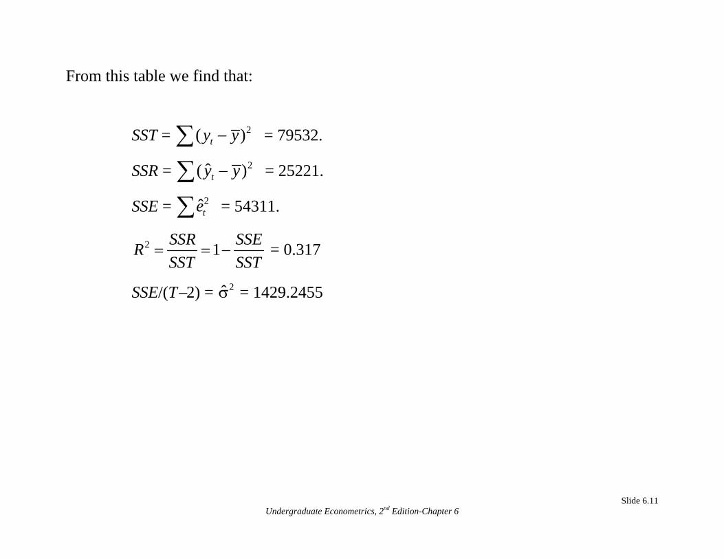
From this table we find that:

SST = 2( ) = 79532. ty y−∑SSR = 2ˆ( ) ty y−∑ = 25221.

SSE = = 54311. 2ˆ te∑2 1SSR SSER

SST SST= = − = 0.317

SSE/(T−2) = = 1429.2455 2σ̂

Slide 6.11


6.1.2 Correlation Analysis

The correlation coefficient ρ between X and Y is

cov( , )var( ) var( )

X YX Y

ρ = (6.1.8)

• Given a sample of data pairs (xt,yt), t=1, ...,T, the sample correlation coefficient is

obtained by replacing the covariance and variances in (6.1.8) by their sample

analogues:

ˆcov( , )垐var( ) var( )

X YrX Y

= (6.1.9)

where


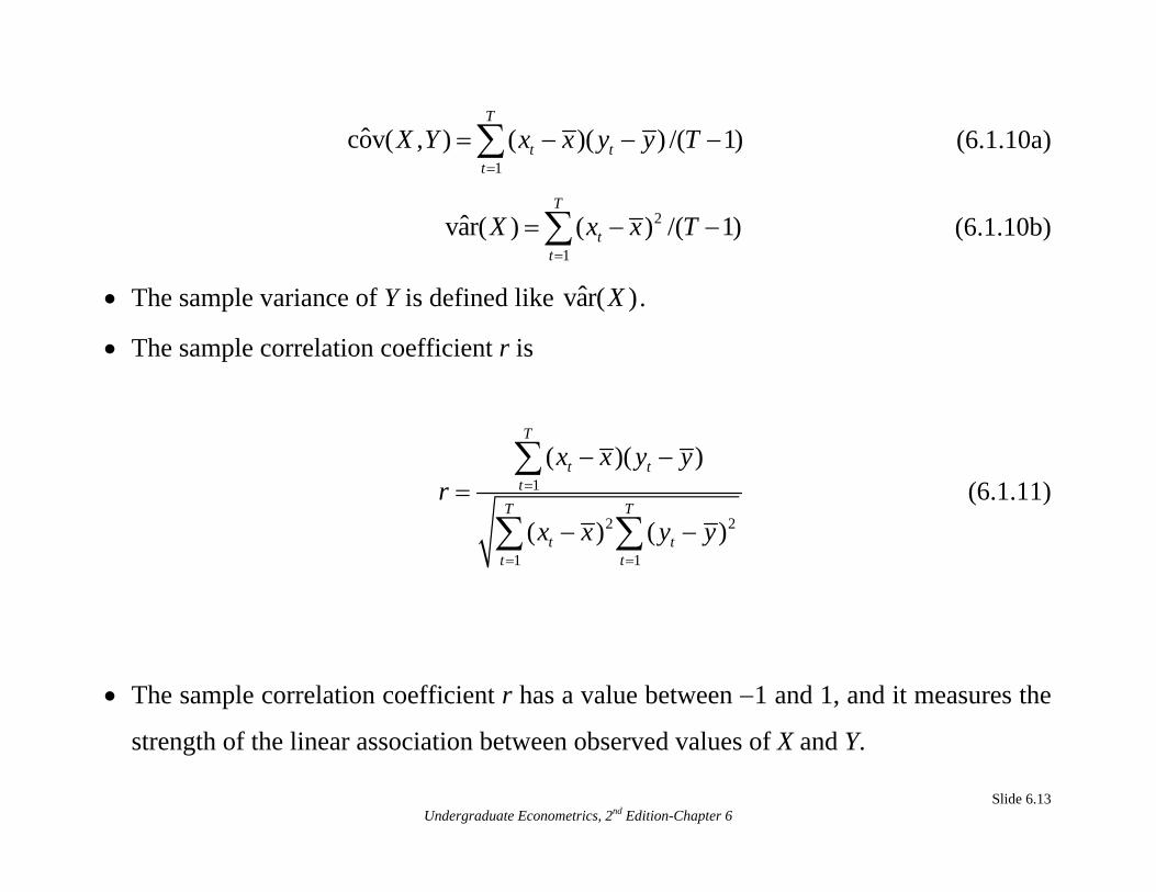
1

ˆcov( , ) ( )( ) /( 1)T

t tt

X Y x x y y T=

= − − − (6.1.10a) ∑

2

1

ˆvar( ) ( ) /( 1)T

tt

X x x T=

= − − (6.1.10b) ∑

• The sample variance of Y is defined like . ˆvar( )X

• The sample correlation coefficient r is

1

2 2

1 1

( )( )

( ) ( )

T

t tt

T T

t tt t

x x y yr

x x y y

=

= =

− −=

− −

∑

∑ ∑ (6.1.11)

• The sample correlation coefficient r has a value between −1 and 1, and it measures the

strength of the linear association between observed values of X and Y.


6.1.3 Correlation Analysis and R2

• There are two interesting relationships between and r in the simple linear

regression model.

2R

Slide 6.14


r =1. The first is that 2R . That is, the square of the sample correlation coefficient

between the sample data values x

2

t and yt is algebraically equal to 2R

2. can also be computed as the square of the sample correlation coefficient between y2R t

and t1 2ˆty b b= + x . As such it measures the linear association, or goodness of fit,

between the sample data and their predicted values. Consequently R2 is sometimes

called a measure of “goodness of fit.”

6.2 Reporting the Results of a Regression Analysis

One way to summarize the regression results is in the form of a “fitted” regression

equation:

2ˆ =40.7676 0.1283 0.317

(s.e.) (22.1387)(0.0305) t ty x R+ =

(R6.6)

• The value b1 = 40.7676 estimates the weekly food expenditure by a household with no

income;

• b2 =0.1283 implies that given a $1 increase in weekly income we expect expenditure

on food to increase by $.13; or, in more reasonable units of measurement, if income

increases by $100 we expect food expenditure to rise by $12.83.

• The =0.317 says that about 32% of the variation in food expenditure about its mean

is explained by variations in income.

2R

Slide 6.15


• The numbers in parentheses underneath the estimated coefficients are the standard

errors of the least squares estimates. Apart from critical values from the t-distribution,

(R6.6) contains all the information that is required to construct interval estimates for β1

or β2 or to test hypotheses about β1 or β2.

• Another conventional way to report results is to replace the standard errors with the “t-

values”

• These values arise when testing H0: β1 = 0 against H1: β1 ≠ 0 and H0: β2 = 0 against H1:

β2 ≠ 0.

• Using these t-values we can report the regression results as

2ˆ 40.7676 0.1283 0.317

( ) (1.84) (4.20) t ty x Rt= + = (6.2.2)

Slide 6.16


6.2.1 The Effects of Scaling the Data

• Data we obtain are not always in a convenient form for presentation in a table or use in

a regression analysis. When the scale of the data is not convenient it can be altered

without changing any of the real underlying relationships between variables.

• For example, suppose we are interested in the variable x = U.S. total real disposable

personal income. In 1999 the value of x = $93,491,400,000,000.

• We might divide the variable x by 1 trillion and use instead the scaled variable

,000= $93.4914 trillion dollars. * /1,000,000,000x x=

• Consider the food expenditure model. We interpret the least squares estimate b2 =

0.1283 as the expected increase in food expenditure, in dollars, given a $1 increase in

weekly income.

Slide 6.17


• It may be more convenient to discuss increases in weekly income of $100. Such a

change in the units of measurement is called scaling the data. The choice of the scale

is made by the investigator so as to make interpretation meaningful and convenient.

• The choice of the scale does not affect the measurement of the underlying relationship,

but it does affect the interpretation of the coefficient estimates and some summary

measures.

• Let us summarize the possibilities:

1. Changing the scale of x:

( )*

ˆ =40.77 0.1283

=40.77+ 100 0.1283 100

=40.77 12.83

t t

t

t

y xx

x

+

⎛ ⎞× ⎜ ⎟ (R6.8) ⎝ ⎠

+

• In the food expenditure model b2 =0.1283 measures the effect of a change in income of

$1 while 100b


2 =$12.83 measures the effect of a change in income of $100.

• When the scale of x is altered the only other change occurs in the standard error of the

regression coefficient, but it changes by the same multiplicative factor as the

coefficient, so that their ratio, the t-statistic, is unaffected. All other regression

statistics are unchanged.

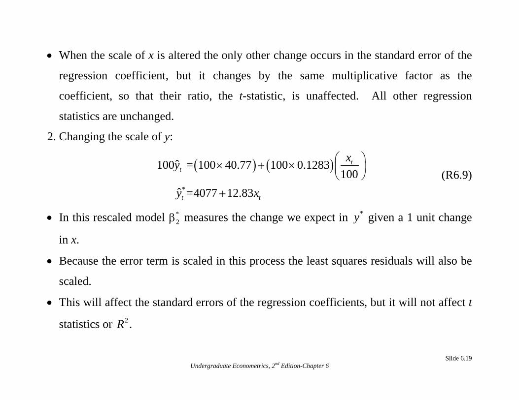
2. Changing the scale of y:

( ) ( )*

ˆ 100 = 100 40.77 100 0.1283 100

ˆ =4077 12.83

tt

t t

xy

y x

⎛ ⎞× + × ⎜ ⎟⎝ ⎠ (R6.9)

+

*y• In this rescaled model measures the change we expect in *2β given a 1 unit change

in x.

• Because the error term is scaled in this process the least squares residuals will also be

scaled.

• This will affect the standard errors of the regression coefficients, but it will not affect t

statistics or . 2R

Slide 6.19


3. If the scale of y and the scale of x are changed by the same factor, then there will be no

change in the reported regression results for b2, but the estimated intercept and

residuals will change; t-statistics and are unaffected. The interpretation of the

parameters is made relative to the new units of measurement.

2R

6.3 Choosing a Functional Form

• In the household food expenditure function the dependent variable, household food

expenditure, has been assumed to be a linear function of household income.

• What if the relationship between y

Slide 6.20


t and xt is not linear?

Remark: The term linear in “simple linear regression model” means not a

linear relationship between the variables, but a model in which the parameters

enter in a linear way. That is, the model is “linear in the parameters,” but it is

not, necessarily, “linear in the variables.”

• By “linear in the parameters” we mean that the parameters are not multiplied together,

divided, squared, cubed, etc.

• The variables, however, can be transformed in any convenient way, as long as the

resulting model satisfies assumptions SR1-SR5 of the simple linear regression model.

• In the food expenditure model we do not expect that as household income rises that

food expenditures will continue to rise indefinitely at the same constant rate.

• Instead, as income rises we expect food expenditures to rise, but we expect such

expenditures to increase at a decreasing rate.

y

x

Figure 6.2 A Nonlinear Relationship between Food Expenditure and Income

Slide 6.21


22


6.3.1 Some Commonly Used Functional Forms

The variable transformations that we begin with are:

1. The natural logarithm: if x is a variable then its natural logarithm is ln(x).

2. The reciprocal: if x is a variable then its reciprocal is 1/x.

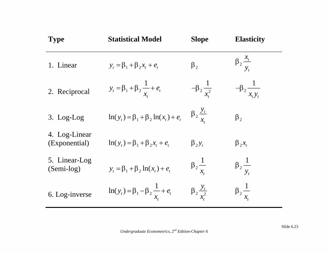
Type Statistical Model Slope Elasticity

2t

t

xy

β

Slide 6.23


1. Linear 1 2t t ty x e= β +β + 2β

1 21

t tt

y ex

= β +β + 2 2

1

tx−β 2

1

t tx y−β

2. Reciprocal 3. Log-Log

1 2ln( ) ln( )t t ty x e= β +β + 2

t

t

yx

β 2β

4. Log-Linear (Exponential)

1 2ln( )t t ty x e= β +β +

2 tyβ 2 txβ

5. Linear-Log (Semi-log)

1 2 ln( )t t ty x e= β +β + 2

1

txβ 2

1

tyβ

1 21ln( )t t

t

y ex

= β −β + 2 2t

t

yx

β 21

txβ

6. Log-inverse

[Figure 6.3 goes here]

1. The model that is linear in the variables describes fitting a straight line to the

original data, with slope and point elasticity t2 /tx y2β β . The slope of the relationship is

constant but the elasticity changes at each point.

2. The reciprocal model takes shapes shown in Figure 6.3(a). As x increases y

approaches the intercept, its asymptote, from above or below depending on the sign of

. The slope of this curve changes, and flattens out, as x increases. The elasticity also

changes at each point and is opposite in sign to 2β

. In Figure 6.3(a), when 2β 2β >0, the

relationship between x and y is an inverse one and the elasticity is negative: a 1%

increase in x leads to a reduction in y of 2 /( )t tx y−β %.

3. The log-log model is a very popular one. The name “log-log” comes from the fact that

the logarithm appears on both sides of the equation. In order to use this model all values

of y and x must be positive. The shapes that this equation can take are shown in Figures

6.3(b) and 6.3(c). Figure 6.3(b) shows cases in which > 0, and Figure 6.3(c) shows 2β

Slide 6.24


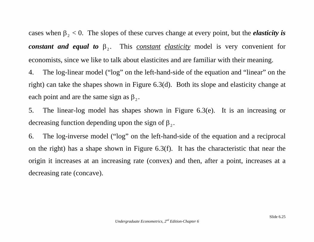
cases when < 0. The slopes of these curves change at every point, but the elasticity is

constant and equal to 2β

Slide 6.25


2β . This constant elasticity model is very convenient for

economists, since we like to talk about elasticites and are familiar with their meaning.

4. The log-linear model (“log” on the left-hand-side of the equation and “linear” on the

right) can take the shapes shown in Figure 6.3(d). Both its slope and elasticity change at

each point and are the same sign as . 2β

5. The linear-log model has shapes shown in Figure 6.3(e). It is an increasing or

decreasing function depending upon the sign of . 2β

6. The log-inverse model (“log” on the left-hand-side of the equation and a reciprocal

on the right) has a shape shown in Figure 6.3(f). It has the characteristic that near the

origin it increases at an increasing rate (convex) and then, after a point, increases at a

decreasing rate (concave).

26


Remark: Given this array of models, some of which have similar shapes, what

are some guidelines for choosing a functional form? We must certainly choose

a functional form that is sufficiently flexible to “fit” the data. Choosing a

satisfactory functional form helps preserve the model assumptions. That is, a

major objective of choosing a functional form, or transforming the variables, is

to create a model in which the error term has the following properties;

1. E(et)=0

2. var(et)=σ2

3. cov(ei,ej)=0

4. et~N(0, σ2)

If these assumptions hold then the least squares estimators have good statistical

properties and we can use the procedures for statistical inference that we have

developed in Chapters 4 and 5.

6.3.2 Examples Using Alternative Functional Forms

In this section we will examine an array of economic examples and possible choices for

the functional form.

6.3.2a The Food Expenditure Model

• From the array of shapes in Figure 6.3 two possible choices that are similar in some

aspects to Figure 6.2 are the reciprocal model and the linear-log model.

• The reciprocal model is

1 21

t tet

yx

= β +β + (6.3.2)

• For the food expenditure model we might assume that β > 0 and β1 2 < 0. If this is the

case, then as income increases, household consumption of food increases at a

decreasing rate and reaches an upper bound β1.


• This model is linear in the parameters but it is nonlinear in the variables. If the error

term et satisfies our usual assumptions, then the unknown parameters can be estimated

by least squares, and inferences can be made in the usual way.

• Another property of the reciprocal model, ignoring the error term, is that when x <

−β2/β1 the model predicts expenditure on food to be negative. This is unrealistic and

implies that this functional form is inappropriate for small values of x.

• When choosing a functional form one practical guideline is to consider how the

dependent variable changes with the independent variable. In the reciprocal model the

slope of the relationship between y and x is

2 2

1

t

dydx x

= −β

If the parameter β2 < 0 then there is a positive relationship between food expenditure and

income, and, as income increases this “marginal propensity to spend on food” diminishes,

as economic theory predicts.

Slide 6.28


• For the food expenditure relationship an alternative to the reciprocal model is the

linear-log model

1 2 ln( )t

Slide 6.29


t ty x eβ +β + (6.3.3) =

which is shown in Figure 6.3(e).

• For β2 > 0 this function is increasing, but at a decreasing rate. As x increases the slope

β2/xt decreases.

• Similarly, the greater the amount of food expenditure y the smaller the elasticity, β2/yt.

6.3.2b Some Other Economic Models and Functional Forms

1. Demand Models: models of the relationship between quantity demanded (yd

Slide 6.30


y = β + β +

y

) and price

(x) are very frequently taken to be linear in the variables, creating a linear demand

curve, as so often depicted in textbooks. Alternatively, the “log-log” form of the

model, t tx e , is very convenient in this situation because of its

“constant elasticity” property. Consider Figure 6.3(c) where several log-log models

are shown for several values of β

1 2ln( ) ln( )dt

2 < 0. They are negatively sloped, as is appropriate

for demand curves, and the price-elasticity of demand is the constant β2.

2. Supply Models: if ys is the quantity supplied, then its relationship to price is often

assumed to be linear, creating a linear supply curve. Alternatively the log-log, constant

elasticity form, t tx e1 2ln( ) ln( )st , can be used = β + β +

3. Production Functions: One of the assumptions of production theory is that

diminishing returns hold; the marginal-physical product of the variable input declines

as more is used. To permit a decreasing marginal product, the relation between output

(y) and input (x) is often modeled as a “log-log” model, with β2 < 1. This relationship

is shown in Figure 6.3(b). It has the property that the marginal product, which is the

slope of the total product curve, is diminishing, as required.

4. Cost Functions: a family of cost curves, which can be estimated using the simple

linear regression model, is based on a “quadratic” total cost curve.

• Suppose that you wish to estimate the total cost (y) of producing output (x); then a

potential model is given by

Slide 6.31


y x21 2t t teβ +β + (6.3.4) =

• If we wish to estimate the average cost (y/x) of producing output x then we might

divide both sides of equation 6.3.4 by x and use

1 2( / ) / /t t t t t

Slide 6.32


ty x x x e xβ +β + (6.3.5) =

which is consistent with the quadratic total cost curve.

5. The Phillips Curve: If we let wt be the wage rate in time t, then the percentage change

in the wage rate is

1

1

% t tt

t

w www

−

−

−Δ = (6.3.6)

is proportional to the excess demand for labor dIf we assume that % twΔ t, we may

write

% t tdw = γ (6.3.7) Δ

where γ is an economic parameter.

• Since the unemployment rate ut is inversely related to the excess demand for labor,

we could write this using a reciprocal function as

1t

t

du

= α +η (6.3.8)

where α and η are economic parameters. Given equation 6.3.7 we can substitute for dt,

and rearrange, to obtain

Slide 6.33


1%

1

tt

t

wu

u

⎛ ⎞Δ = γ α + η⎜ ⎟

⎝ ⎠

= γα + γη

This model is nonlinear in the parameters and nonlinear in the variables.

Slide 6.34


to complete the analysis of the simple linear regression model…econ446/wiley/chapter6.pdf · ·...

Documents