title the evolution and intensification of cyclone pam

RIGHT:

URL:

CITATION:

AUTHOR(S):

ISSUE DATE:

TITLE:

The evolution and intensification ofCyclone Pam (2015) and resultingstrong winds over the southernPacific islands

Takemi, Tetsuya

Takemi, Tetsuya. The evolution and intensification of Cyclone Pam (2015) and resultingstrong winds over the southern Pacific islands. Journal of Wind Engineering & IndustrialAerodynamics 2018, 182: 27-36

2018-11

http://hdl.handle.net/2433/234587

© 2018. This manuscript version is made available under the CC-BY-NC-ND 4.0 licensehttp://creativecommons.org/licenses/by-nc-nd/4.0/; The full-text file will be made open to the public on 01 November2020 in accordance with publisher's 'Terms and Conditions for Self-Archiving'.; この論文は出版社版でありません。引用の際には出版社版をご確認ご利用ください。; This is not the published version. Please cite only the publishedversion.

The evolution and intensification of Cyclone Pam (2015) and

resulting strong winds over the southern Pacific islands

Tetsuya Takemi

Disaster Prevention Research Institute, Kyoto University, Uji, Kyoto, Japan

Corresponding author:Tetsuya Takemi, Disaster Prevention Research Institute, Kyoto University, Gokasho, Uji, Kyoto 611-0011, Japan.E-mail: [email protected]

A Self-archived copy inKyoto University Research Information Repository

https://repository.kulib.kyoto-u.ac.jp

1

ABSTRACT1 Cyclone Pam (2015), a category-5 storm, in the southern Pacific in March 2015 caused 2 severe damages over the islands states in the southern Pacific. Cyclone Pam was originated 3 from an active convective region in the Madden-Julian oscillation (MJO) and evolved from 4 convective clouds into a tropical cyclone. This study numerically investigated the effects of 5 convective processes on the evolution and intensification of Cyclone Pam and the resulting 6 strong winds with the use of the Weather Research and Forecasting (WRF) model through 7 examining sensitivities to cloud microphysics schemes. The numerical simulations 8 successfully reproduced the eastward propagation of the MJO and the aggregation of 9 convective clouds that transformed to a tropical cyclone. It was found that microphysics

10 processes affect the diabatic heating and therefore the evolution of tropical convection into 11 a tropical cyclone. The potential instability for convective development and the actual 12 development of deep cumulus clouds both contribute to the sensitivity of the simulated TC 13 to the choice of the cloud microphysics schemes. Even with such sensitivity, this study 14 successfully reproduced the cyclone track accurately in all the experiments and therefore is 15 able to generate consistent hazard information from the cyclone.16

17 Keywords: tropical cyclone; typhoon hazard; meteorological modeling; wind-related 18 disasters; impact assessment19

20 1. Introduction21

22 Tropical cyclones (TCs) are one of the major meteorological hazards and sometimes produce 23 heavy rainfalls, strong winds, high waves, and storm surge. When TCs hit regions which are 24 vulnerable to natural hazards, the impacts of TCs on human lives, social infrastructures, and 25 economic activities will be enormous. Still recently there have been TCs that spawned 26 devastating damages. For example, Cyclone Sidr (2017) landed on the southwestern coast of 27 Bangladesh in November 2007, causing more than 3000 fatalities and huge economic damages 28 (Paul, 2009). Cyclone Nargis (2008) made landfall on the Irrawaddy delta region of Myanmar 29 in May 2008 and caused a devastating disaster that is regarded as the most damaging in the 30 recorded history of Myanmar (Webster, 2008). Typhoon Haiyan (2013) made landfall on the 31 Philippines in November 2013 and spawned severe storm surges over the coastal area of the 32 Leyte Gulf. The central surface pressure of Typhoon Haiyan reached 895 hPa at its mature stage 33 and is a category-5 storm in the Saffir-Simpson scale. To prepare for more extreme TCs, Lin et 34 al. (2014) proposed that an extreme category above category 5, i.e., category 6 is required within 35 the Saffir-Simpson scale. Not only to prepare for the coming TCs every year but also to respond 36 to the anticipated increase in the intensity of TCs under future global warming, mitigating 37 disaster risks from TCs is a critical social issue for those regions.38 Another recent TC that severely affected developing countries is Cyclone Pam (2015), which



2

39 developed in the southern tropical Pacific in March 2015. Cyclone Pam caused severe damages 40 over the islands states in the southern Pacific. According to the information by Joint Typhoon 41 Warning Center (JTWC), Cyclone Pam was a category-5 storm and its maximum wind speed 42 reached about 75 m s-1. Among the region affected, the islands of Vanuatu were severely 43 damaged by the cyclone. The damages by Cyclone Pam are regarded as the worst natural 44 disaster in the history of Vanuatu (Vitart et al., 2017). Because the isolated islands in the open 45 ocean are susceptible to strong winds, high waves, and storm surges, a quantitative assessment 46 of hazards induced by TCs is important in order to mitigate and prevent resulting disasters. The 47 quantitative assessment of the hazard specific to this cyclone should enhance the resilience of 48 the society of the islands states by designing appropriate measures for future cyclone hazards.49 In addition, this cyclone is of meteorological interest, because Cyclone Pam developed and 50 evolved from an active convective phase of a Madden-Julian Oscillation (MJO) signal. MJO is 51 a large-scale cluster of convective clouds in the tropics (Madden and Julian, 1971, 1972; Zhang, 52 2005) and sometimes affects the generation and evolution of tropical cyclones by changing the 53 atmospheric conditions favorable for tropical cyclogenesis (Liebmann et al., 1994; Bessafi and 54 Wheeler, 2006; Kim et al., 2008; Camargo et al., 2009; Chand and Walsh, 2010; Kikuchi and 55 Wang, 2010; Huang et al., 2011; Yanase et al., 2012; Klotzbach and Blake, 2013; Klotzbach, 56 2014; Tsuboi and Takemi, 2014). With the use of an index that describes the potential for 57 tropical cyclogenesis (Murakami et al., 2011), it was found that the increase in humidity is an 58 important condition favorable for the generation of tropical cyclones in the Indian Ocean during 59 the active periods of MJO (Tsuboi and Takemi, 2004; Tsuboi et al., 2016). Klotzbach and Blake 60 (2013) indicated that during the convectively active phase of the MJO over the eastern and 61 central tropical Pacific the north-central Pacific tends to have more TCs and the convectively 62 active phase of MJO is responsible for north-central Pacific TCs that experience rapid 63 intensification. Chand and Walsh (2010) examined the modulation of TC genesis by MJO in 64 the central South Pacific (i.e., the Fiji, Samoa, and Tonga regions) and showed that the TC 65 genesis is significantly enhanced during the active phase of MJO. Thus, the intensification of 66 Cyclone Pam that occurred in the central South Pacific is considered to be significantly affected 67 by the presence of MJO. The physical processes that lead to the intensification of Pam are 68 therefore of scientific interest.69 This study numerically investigates the evolution and intensification of Cyclone Pam (2015) 70 that transformed from convective populations to a tropical cyclone by conducting dynamical 71 downscaling simulations with the use of a regional meteorological model, the Weather 72 Research and Forecasting (WRF) model (Skamarock et al., 2008). In order to elucidate the 73 diabatic heating processes that control the development of convective clouds, the sensitivities 74 to the cloud microphysics schemes were investigated. Ice-phase processes are known to affect 75 the development of TCs (Lord et al., 1984; Sawada and Iwasaki, 2007; Fovell et al., 2016). We 76 will demonstrate how the cloud microphysics influences the evolution of convective 77 populations and the intensification to a tropical cyclone and hence affects the assessment of



3

78 hazards by the cyclone. Furthermore, previous studies indicated that a dynamical downscaling 79 simulation with a regional meteorological model is an effective tool to assess the impacts of 80 extreme weather phenomena on local-scale hazards (Mori and Takemi, 2016; Takemi et al., 81 2016a) and has been successfully used for assessing the impacts of typhoons (Ishikawa et al., 82 2013; Oku et al., 2014; Mori et al., 2014; Murakami et al., 2015; Murata et al., 2015; Ito et al., 83 2016; Takano et al., 2016; Takemi et al., 2016b, 2016c). Another purpose of this study, 84 therefore, is to demonstrate the applicability of the dynamical downscaling approach in 85 estimating strong wind hazards by a TC in the southern Pacific.86 This paper is organized as follows. In section 2, the settings of the WRF model and the design 87 of the numerical experiments are described. Section 3 firstly evaluates the performance of the 88 numerical experiments and then examines the evolution of Cyclone Pam from the sensitivity 89 experiments. We will further demonstrate hazards due to cyclone winds in Vanuatu from the 90 dynamical downscaling experiments. We will discuss the advantages and significance of this 91 study by comparing the previous studies in section 4 and will conclude this study in section 5.92

93 2. Numerical model and experimental design94

95 The numerical model used here was the WRF model-the Advanced Research WRF (ARW) 96 version 3.3.1. The model was configured in a realistic mode to simulate the genesis, evolution, 97 and movement of Cyclone Pam under actual meteorological conditions in March 2015.98 During this period, the active convective regions of MJO propagated eastward from the 99 western part of the Indian Ocean to the eastern part of the Pacific. Therefore, the complete

100 description of the MJO in numerical simulations requires a vast computational domain. At the 101 same time, convective nature of MJO requires a sufficient resolution that can represent the 102 organization of convective clouds. However, to meet both the vast computational domain and 103 the convection-resolving grid spacing is not affordable from a viewpoint of computational 104 resources. Thus, two-way nesting capability was used to resolve the active convective regions 105 of MJO and the evolution of the tropical cyclone at a convection-permitting grid spacing in a 106 limited domain that is nested in a coarser-resolution, larger domain. The outer domain (Domain 107 1) covered the tropical regions from the Maritime Continent to the eastern part of the Pacific 108 with an area of 7650 km (east-west) by 4500 km (north-south), centered at . The 152°E, 12°S109 inner domain (Domain 2) covered the central part of the Pacific with an area of 2500 km by 110 3000 km. The map projection of the computational domains was based on the Mercator.111 The spatial resolutions of the simulations were set as follows. The horizontal grid spacings 112 of Domain 1 and 2 were 6 km and 2 km, respectively. While in the vertical, the number of the 113 model levels was 56, and the model top was set to the 20-hPa height. The vertical resolution at 114 the lowest level was 69 m, and there were 8 levels in the lowest 1-km depth. With this vertical 115 resolution, it was expected to sufficiently resolve the low-level inflows of the simulated tropical 116 cyclones. The vertical resolution was gradually stretched with height. There were 20 levels in



4

117 the lowest 3-km depth, and the vertical resolution at around the 3-km height was about 200 m. 118 The vertical resolution was further stretched: about 300 m at around the 5-km height, about 500 119 m at around the 10-km height, and greater than 1 km above the 15-km height.120 The model topography was generated with the use of the global digital elevation model data, 121 GTOPO30, having a horizontal grid spacing of 30 arc-seconds (about 1 km), provided by the 122 United States Geological Survey.123 The physics options employed in the present simulations were chosen based on our recent 124 studies on tropical cyclones (Mori et al., 2014; Mori and Takemi, 2016; Takemi et al., 2016b; 125 Takemi et al., 2016c); for example, we chose the Yonsei University scheme for boundary-layer 126 mixing (Hong et al., 2006) and a Monin-Obukhov similarity-based scheme for surface fluxes 127 (Jimenez et al., 2012). Among the physics processes, the cloud microphysics process affects 128 the diabatic heating due to phase changes and thus is considered to determine the development 129 of convective cloud. Therefore, this study focuses on the sensitivity of the simulated cyclone to 130 the choice of cloud microphysics schemes. The schemes examined here are a single-moment, 131 six-category scheme by Hong and Lim (2006) and two double-moment schemes, i.e., the 132 schemes by Thompson et al. (2008) and Morrison et al. (2009). Brief descriptions of these 133 schemes can be found in the User’s Guide of the WRF model (available online at 134 http://www2.mmm.ucar.edu/wrf/users/docs/user_guide_V3/contents.html) as well as in the 135 technical document (Skamarock et al., 2008). In this study, we conducted three numerical 136 experiments by changing the cloud microphysics scheme but with otherwise the same model 137 settings. The numerical experiments with the single-moment scheme, the Thompson scheme, 138 and the Morrison scheme are respectively referred to as WSM6, THOM, and MORR.139 As the initial and boundary conditions, we used the 6-hourly, 1-degree by 1-degree resolution 140 Final Analysis (FNL) data of National Centers for Environmental Prediction (NCEP) 141 Operational Model Global Tropospheric Analyses. The FNL datasets includes not only three-142 dimensional atmospheric fields but also surface parameters such as sea surface temperature, 143 ground surface temperature, etc. The spectral nudging for low wave-number components (i.e., 144 wave number 2) of middle- and upper-level winds was applied in Domain 1 to keep the 145 synoptic-scale influences on the simulated atmospheric fields. The time coefficient for the 146 spectral nudging was set to 0.00028 s-1. This coefficient was used in the studies of Mori et al. 147 (2014), Ito et al. (2016), and Takemi et al. (2016b, 2016c) who demonstrated that by trial and 148 error the spectral nudging with that coefficient was effective in reproducing the tracks and 149 intensity of typhoons. For this reason, this study also used the same time coefficient.150 It is noted that the present simulations use only the analysis fields but not the forecast fields. 151 Because the analysis fields incorporate observed data through data assimilation technique, they 152 are able to represent large-scale and/or synoptic-scale atmospheric phenomena such as tropical 153 waves, MJO, monsoon, etc. By using the analysis fields and employing spectral nudging to 154 keep the large-scale features into a regional model, the dynamical downscaling approach has 155 advantages in accurately reproducing both large-scale/synoptic-scale phenomena and



5

156 mesoscale disturbances and in quantitatively representing the mesoscale disturbances and the 157 resulting hazards at a high spatial resolution. These advantages are critically important in 158 assessing the disaster impacts at regional scales.159 All the time integrations were started at 0000 UTC 3 March 2015 for Domain 1 and 0000 160 UTC 7 March 2015 for Domain 2 and ended at 0000 UTC 15 March 2015. The simulated 161 outputs were produced at 1-hour interval.162

163 3. Results164

165 3.1. Validation of the numerical experiments166

167 To derive quantitative information of TC hazards, accurate reproductions of the track, 168 intensity, and translation speed of TCs are critically important (Takemi et al., 2016a). From the 169 case of Typhoon Haiyan (2013), it was found that a slight departure of those TC properties in 170 numerical simulations results in large differences of the simulated storm surges in the Leyte 171 Gulf from the actual measurements (Mori et al., 2014). A better reproduction of such TC 172 properties is critical in better assessments of the TC impacts. Here we examine the overall 173 performance of the simulated cyclone from a viewpoint of impact assessments.174 Figure 1 shows the tracks of the observed (from the JTWC best track data) and the simulated 175 tropical cyclone. The simulated results are those obtained by WSM6. At an initial stage when 176 the TC was located near the equator, the locations of the simulated cyclone meander around the 177 region of the latitude near the line and do not seem to agree well with the 10° ‒ 5°S 170°E178 best track. This is because the simulated tropical cyclone at this stage was in a pre-formative 179 phase and thus the organized structure of a tropical cyclone was not seen. Besides, the cyclone 180 winds are not severe at this stage and are not a threat to the surrounding region. Thus, this 181 disagreement can be acceptable. After this initial stage, the simulation well reproduced the track 182 very close to the actual track of Cyclone Pam. Since wind speeds due to TCs strongly depend 183 on the tracks, a close reproduction of the actual tropical cyclone leads to better representations 184 of the hazard information.185 Figure 2 compares the time series of the intensity of the simulated tropical cyclones obtained 186 by the WSM6, THOM, and MORR experiments. The maximum wind speed is available in the 187 JTWC best-track dataset and hence its time series is also indicated. According to the JTWC 188 data, Cyclone Pam reached a tropical storm intensity at 0600 UTC 9 March 2015 and became 189 a tropical cyclone intensity at 0000 UTC 10 March. Overall, in terms of the maximum wind 190 speed (Fig. 2a) the simulations are able to capture the evolution of the tropical cyclone. The 191 peak wind speed of 75 m s-1, however, was not quantitatively captured. In general, the 192 quantitative reproduction of surface wind speed in meteorological model simulations is difficult 193 (Oku et al., 2010; Nakayama et al., 2012), because meteorological models include various types 194 of artificial filters to avoid computational instability (Takemi and Rotunno, 2003; Bryan et al.,



6

195 2005). In some models, steep slopes in complex terrains are smoothed out in order to make the 196 forecast simulations computationally stable, which also diminishes a fluctuating nature of 197 surface winds (Oku et al., 2010). If complex topography is properly represented in 198 meteorological models with sufficient resolutions, there is a chance that fluctuating winds 199 induced by complex topography such as downslope winds, mountain waves, and other 200 dynamically generated turbulent effects can be quantitatively reproduced (Takemi, 2013; 201 Poulidis et al., 2017). In the present study, the surface condition was basically the ocean, and 202 thus, wind fluctuations by surface topography is not expected. Furthermore, the maximum 203 intensity of the simulated tropical cyclones will also depend on the model resolutions (Bryan 204 and Rotunno, 2009). The horizontal grid spacing of 2 km in this study may not be sufficient to 205 quantitatively represent the wind gusts and peaks. With these considerations in mind, the 206 present simulations are regarded as favorable. 207 The time series in Fig. 2 indicate that among the three experiments the MORR experiment 208 produces a cyclone with slower evolution and weaker mature-stage intensity than the WSM6 209 and THOM experiments. The comparison of the radii of the maximum wind speed during the 210 mature stage among the experiments indicates that the radius in the MORR case is a little larger 211 than in the other two cases, which is related to a weaker intensity in the MORR case than in the 212 others.213 The spatial structure of the simulated TC at its mature stage in Domain 2 of the WSM6 case 214 is demonstrated in Fig. 3, which indicates the radar reflectivity at the 2-km height as well as the 215 surface pressure. The simulated time at 1200 UTC 12 March 2015, almost at the time of the 216 maximum intensity, was chosen here. A clockwise distribution of the cyclone eyewall as well 217 as spiraling rainbands outside the eyewall is clearly seen.218 Table 1 summarizes the intensity and size of the simulated tropical cyclones at their 219 maximum intensities obtained in the three experiments. Among the cases examined, the THOM 220 case produced the most intense tropical cyclone and the most compact inner core, although the 221 differences between the THOM and WSM6 cases seem to be minor. The MORR case produced 222 the weakest and the least-compact cyclone.223 Owing to the unavailability of surface meteorological data during the passage of Cyclone 224 Pam, this study can provide only the information described here. It is very difficult to evaluate 225 the performance of the meteorological model simulations by surface meteorological data in 226 regions with sparsely distributed islands in the open ocean. By considering that the simulations 227 are able to capture the track and intensity of the actual TC, we will use the simulated data to 228 investigate the processes leading to the intensification and development of Cyclone Pam and to 229 estimate the strong wind hazards at local scales in the following sections.230

231 3.2. Evolutionary processes of Cyclone Pam (2015)232

233 According to the diagnosis on the MJO activity in terms of the real-time multivariate MJO



7

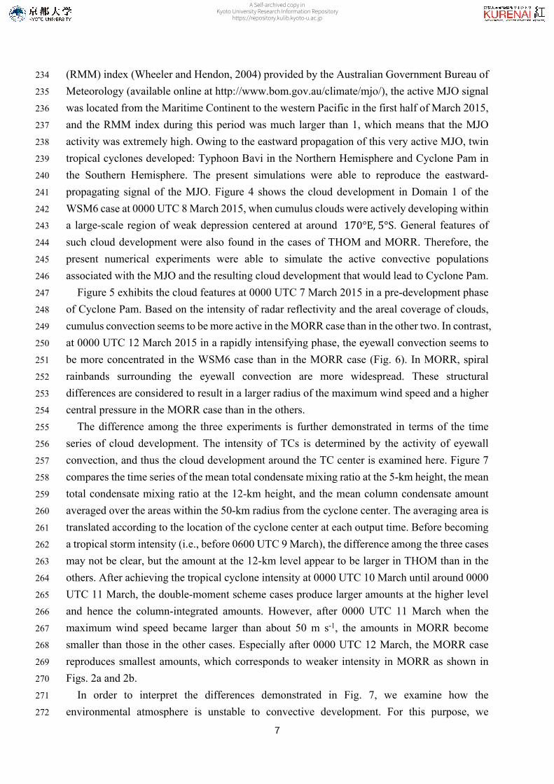
234 (RMM) index (Wheeler and Hendon, 2004) provided by the Australian Government Bureau of 235 Meteorology (available online at http://www.bom.gov.au/climate/mjo/), the active MJO signal 236 was located from the Maritime Continent to the western Pacific in the first half of March 2015, 237 and the RMM index during this period was much larger than 1, which means that the MJO 238 activity was extremely high. Owing to the eastward propagation of this very active MJO, twin 239 tropical cyclones developed: Typhoon Bavi in the Northern Hemisphere and Cyclone Pam in 240 the Southern Hemisphere. The present simulations were able to reproduce the eastward-241 propagating signal of the MJO. Figure 4 shows the cloud development in Domain 1 of the 242 WSM6 case at 0000 UTC 8 March 2015, when cumulus clouds were actively developing within 243 a large-scale region of weak depression centered at around . General features of 170°E, 5°S244 such cloud development were also found in the cases of THOM and MORR. Therefore, the 245 present numerical experiments were able to simulate the active convective populations 246 associated with the MJO and the resulting cloud development that would lead to Cyclone Pam.247 Figure 5 exhibits the cloud features at 0000 UTC 7 March 2015 in a pre-development phase 248 of Cyclone Pam. Based on the intensity of radar reflectivity and the areal coverage of clouds, 249 cumulus convection seems to be more active in the MORR case than in the other two. In contrast, 250 at 0000 UTC 12 March 2015 in a rapidly intensifying phase, the eyewall convection seems to 251 be more concentrated in the WSM6 case than in the MORR case (Fig. 6). In MORR, spiral 252 rainbands surrounding the eyewall convection are more widespread. These structural 253 differences are considered to result in a larger radius of the maximum wind speed and a higher 254 central pressure in the MORR case than in the others.255 The difference among the three experiments is further demonstrated in terms of the time 256 series of cloud development. The intensity of TCs is determined by the activity of eyewall 257 convection, and thus the cloud development around the TC center is examined here. Figure 7 258 compares the time series of the mean total condensate mixing ratio at the 5-km height, the mean 259 total condensate mixing ratio at the 12-km height, and the mean column condensate amount 260 averaged over the areas within the 50-km radius from the cyclone center. The averaging area is 261 translated according to the location of the cyclone center at each output time. Before becoming 262 a tropical storm intensity (i.e., before 0600 UTC 9 March), the difference among the three cases 263 may not be clear, but the amount at the 12-km level appear to be larger in THOM than in the 264 others. After achieving the tropical cyclone intensity at 0000 UTC 10 March until around 0000 265 UTC 11 March, the double-moment scheme cases produce larger amounts at the higher level 266 and hence the column-integrated amounts. However, after 0000 UTC 11 March when the 267 maximum wind speed became larger than about 50 m s-1, the amounts in MORR become 268 smaller than those in the other cases. Especially after 0000 UTC 12 March, the MORR case 269 reproduces smallest amounts, which corresponds to weaker intensity in MORR as shown in 270 Figs. 2a and 2b.271 In order to interpret the differences demonstrated in Fig. 7, we examine how the 272 environmental atmosphere is unstable to convective development. For this purpose, we



8

273 computed convective available potential energy (CAPE), which is a measure to quantify the 274 instability of the density stratification of the tropospheric environment for convective 275 development. The accumulation of CAPE around the TC center is important for the 276 intensification of TCs (Miyamoto and Takemi, 2013, 2015), and thus the environmental CAPE 277 values are examined. Here CAPE values were averaged in areas within the radius of either 500 278 km or 100 km from the TC center along the TC track at times 12 hour prior to the TC arrival. 279 Figure 8 shows the temporal changes of the CAPE values from 0000 UTC 7 March to 0000 280 UTC 14 March for the three experiments. The time series of CAPE computed in the both areas 281 indicate that the values are overall larger in WSM6 and THOM than in MORR at the earlier 282 stage for the 100-km radius area and almost throughout the time period for the 500-km radius 283 area. The CAPE values in the 500-km radius area demonstrate a steadily changing feature in 284 time, compared with those in the 100-km radius area, and clearly indicate that there are 285 differences in the environmental instability among the three experiments. This behavior 286 suggests that CAPE evaluated in a sufficiently larger region is regarded as a guide to properly 287 diagnose the environmental conditions.288 From these analyses, the potential instability for convective development and the actual 289 development of deep cumulus clouds both contribute to the sensitivity of the simulated TC to 290 the choice of the cloud microphysics schemes.291

292 3.3. Assessment of strong wind hazards293

294 From the successful reproduction of the actual tropical cyclone in the numerical experiments 295 as well as the demonstrated sensitivity of the simulated results to the cloud microphysics 296 schemes, we are able to show robustness and possible uncertainty regarding strong wind hazard 297 caused by the present specific cyclone. Strong wind hazard is estimated in terms of the 298 maximum surface wind speed at each grid point from the time series during the simulated time 299 period of Domain 2.300 Figure 9 shows the spatial distributions of the maximum surface wind speed at each grid 301 point in the region of the Vanuatu islands, obtained in Domain 2 of the three experiments. As 302 summarized in Table 1, the strongest intensity was found in the THOM case. Consistent with 303 this, it is seen from Fig. 9 that the strongest wind speeds among the experiments are reproduced 304 in the THOM case and those in the WSM6 case follows. Note here that the simulated outputs 305 at 1-hour interval were used to create Figure 9 and thus the distribution appears to be 306 discontinuous. This discontinuous appearance is actually not related to physical processes. A 307 common feature among the three experiments is that the areas susceptible to strong winds of 308 greater than 45 m s-1 are Efate Island, located around , and the southeastern 168.5°E, 17.5°S309 islands, especially the eastern side of these islands, located to the southeast of Efate Island. 310 Besides, the width of the strong wind area is concentrated, because of the compact size of the 311 cyclone inner core (as shown by the radius of the maximum wind in Table 1).



9

312 Such a qualitative feature common to the three experiments was due to the similar simulated 313 tracks of the cyclone in these experiments. As pointed out by Takemi et al. (2016a), reproducing 314 consistent tracks of TCs in numerical simulations is critically important in assessing natural 315 hazards induced by TCs. In this sense, the present study successfully reproduced the cyclone 316 track accurately in all the sensitivity experiments and therefore is able to generate consistent 317 hazard information from the cyclone. In other words, a regional meteorological model 318 simulation can be a useful tool to assess the impacts of TCs on local-scale hazards if the 319 simulation can well capture the track and intensity of the TCs.320

321 322 4. Discussion323

324 The present numerical experiments successfully reproduced the clustering of convective 325 populations during the active phase of MJO and the transition and evolution to Cyclone Pam in 326 March 2015, and generally captured the intensity and track of the cyclone. MJO is a large-scale 327 atmospheric signal that has a spatial scale of several 1000 km or larger, while a TC has a spatial 328 scale of less than 1000 km. Thus, representing both MJO and TC in numerical models requires 329 a larger computational domain that can cover the ocean-basin scales and a high spatial 330 resolution that can represent convective clouds. Furthermore, reproducing closely the track and 331 intensity of TCs in numerical models is crucial from an impact assessment perspective (Mori 332 and Takemi, 2016; Takemi et al., 2016a).333 Nakano et al. (2017) conducted numerical simulations of Cyclone Pam (2015) by using a 334 non-hydrostatic, global atmospheric model and investigated the influence of sea surface 335 temperature on the MJO and the modulation of the cyclone in March 2015. They successfully 336 simulated the large-scale atmospheric features surrounding the cyclone, but did not examine 337 the track and intensity of Pam, probably because of a coarse resolution (i.e., 14 km). Wang et 338 al. (2015) conducted regional simulations of MJO activity for the two months period from 339 October to November 2011 and indicated that the TC events observed during the period are 340 closely related to the northward propagation of MJO events. However, because the horizontal 341 grid spacing of the simulations was 9 km, TC were not quantitatively represented in terms of 342 the track, intensity, and structure. There are some studies that performed regional simulations 343 at a few km resolution. Hogsett and Zhang (2010) used a moving, nested domain at the 2-km 344 grid to track the evolution of a TC in the western North Pacific, while Fang and Zhang (2016) 345 employed a grid spacing of 1.5 km in the innermost nested domain to simulate a supertyphoon 346 in the western North Pacific. Even with such a convection-permitting resolution (i.e., a few km 347 spacing), they did not examine how the track and intensity of the simulated TCs were 348 quantitatively reproduced.349 In this way, there have been some challenges to reveal the mechanisms for the influences of 350 MJO on the development and evolution of TCs from a viewpoint of basic meteorology.



10

351 However, to our knowledge, there are not a sufficient number of studies on how meteorological 352 models perform the TC evolution under strong influences of MJO from an impact assessment 353 point of view, although the influences of MJO appear in the tropical regions from the Indian 354 Ocean to the Pacific which are vulnerable to cyclone hazards and have high risks of disasters 355 from such hazards. Presenting strong wind hazards with acknowledging the uncertainties 356 resulting from the parameterized physics processes in meteorological models is an advantage 357 and significance of this study.358 As far as the impact of cloud microphysics is concerned, Van Weverberg et al. (2013) 359 investigated the role of the cloud microphysics in the simulations of mesoscale convective 360 systems (MCSs) in the tropical western Pacific by examining the impacts of setting the cloud 361 microphysics scheme to either the Hong and Lim scheme (WSM6) or the Thompson et al. 362 scheme (THOM) or the Morrison et al. scheme (MORR), the same three schemes examined in 363 this study. They demonstrated that the simulation of MCSs is very sensitive to the microphysics 364 parameterization. Specifically, they found that microphysics schemes with slower fallout of 365 upper-level ice lead to a larger buildup of condensate and finally to larger anvils extending from 366 the updraft cores. In their experiments, the MORR and THOM cases produced larger MCSs 367 than the WSM6 case; however, the mechanisms for the larger MCSs in the MORR and THOM 368 cases are different. In MORR abundant slowly falling cloud ice particles play a role, while in 369 THOM very small and slowly falling snowflakes play a role.370 Such a different mechanism in producing larger MCSs between the Morrison and Thompson 371 schemes is considered to play a role in the early phase or before this early phase of the present 372 cyclone. Because the mixing ratio of snow is generally larger than that of cloud ice (see Fig. 8 373 of Van Weverberg et al. (2013)), the larger amount of the total condensate at the 12-km height 374 in the present THOM case (Fig. 7) is considered to be due to the presence of a larger amount of 375 snow. In contrast, the present MORR case produced a larger amount of the total condensate at 376 the 5-km height. Actually, before 0000 UTC 7 March 2015 the total condensate at the 5-km 377 height was the largest in MORR among the three experiments, and therefore, the cumulus 378 convection was generally more active in MORR than in the other two cases not only in the early 379 stage (Fig. 5) but also before 7 March 2015 (not shown). Because active convection overturn 380 the unstable stratification, the atmosphere becomes more stable in MORR than in the other two 381 cases. This is consistent with the smallest value of CAPE in the MORR case among the three 382 cases not only in the early phase but also in the intensifying phase (Fig. 8). Such smallest CAPE 383 in MORR was originated before 0000 UTC 7 March: CAPE in MORR was around 2000 J kg-1 384 while that in THOM and WSM6 was around 3000 J kg-1 during the period from 0000 UTC 3 385 March to 0000 UTC 7 March. Therefore, more active convection before the development of the 386 cyclone make the atmosphere more stable, resulting in a weaker cyclone at its mature stage (in 387 the MORR case), while more suppressed convection before the development of the cyclone 388 leads to a buildup of unstable energy, resulting in a stronger cyclone with a more rapidly 389 intensifying stage (in the WSM6 and THOM cases).



11

390 Of course, these differences depend on the comparison among the three cases examined here, 391 and it should be noted that all the cases reproduced category-5 cyclones at their mature stage. 392 By considering that in the study of Van Weverberg et al. (2013) the Thompson scheme 393 produced the most realistic MCS properties, the THOM case in this study may have a reliability 394 in reproducing the actual properties of Cyclone Pam. However, cloud microphysics processes 395 have a close relationship with radiative heating, and hence the cloud-radiative feedbacks should 396 be carefully examined (Fovel et al., 2016). Currently, based on the previous studies we are not 397 able to give satisfactory conclusions to quantify the influences of cloud microphysics processes 398 on the development and intensification of TCs. An important point here is that the quantitative 399 assessment of cyclone hazards requires understanding the uncertainties resulting from the 400 physical processes parameterized in meteorological models including the cloud microphysics 401 processes.402

403

404 5. Conclusions405

406 The present study investigated the generation and evolution of Cyclone Pam (2015) by using 407 a regional-scale meteorological model, the WRF model, and estimated the impacts of this 408 specific cyclone on the local-scale hazards. The sensitivities to the cloud microphysics schemes, 409 i.e., a single-moment scheme (WSM6), and double-moment schemes (the Thompson and the 410 Morrison schemes), were investigated by performing nested regional simulations at 6- and 2-411 km horizontal resolutions.412 All the numerical simulations successfully reproduced the eastward propagation of the MJO. 413 In the southern part of the convective active region of the MJO, the aggregation of convective 414 clouds was well simulated in all the experiments. A difference was found in the point that the 415 most detailed (Morrison) scheme produced wider-spread areas of convective clouds than the 416 other two schemes. This difference plays a relatively minor role in aggregating convective 417 clouds in the initial stage before the development of the tropical cyclone. However, this small 418 difference affects the temporal evolution from the convective aggregation into a tropical 419 cyclone, which results in slower evolution and a weaker storm in the Morrison scheme. 420 Microphysics processes affects the diabatic heating and therefore the evolution of tropical 421 convection into a tropical cyclone.422 Diagnosis of the environmental conditions before the TC arrival indicated that the 423 environment in WSM6 and THOM is more unstable than that in MORR. From this result as 424 well as the evolution of cumulus clouds, it is considered that the potential instability for 425 convective development and the actual development of deep cumulus clouds both contribute to 426 the sensitivity of the simulated TC to the choice of the cloud microphysics schemes.427 From the analysis of pointwise maximum wind speed at the surface, the present simulations 428 are able to generate robust hazard information over the Vanuatu islands, irrespective of the



12

429 choice of the cloud microphysics schemes. The present study successfully reproduced the 430 cyclone track accurately in all the sensitivity experiments and therefore is able to generate 431 consistent hazard information from the cyclone.432 In the tropics, TCs and other meteorological disturbances sometimes induce severe local 433 storms that may harm human lives and societies in regions vulnerable to natural disasters. Like 434 Cyclone Pam (2015), severe storms such as high winds and heavy rainfall are generated 435 sometimes in association with MJO. Takemi (2015) also conducted downscaling numerical 436 simulations of MJO over the tropical Indian Ocean for the two months period in October and 437 November 2011 and successfully reproduced active cumulus convection during the active phase 438 of MJO. Based on the present simulations as well as those shown in Takemi (2015), it is 439 emphasized that a dynamical downscaling approach with the use of a regional meteorological 440 model is useful in quantitatively assess meteorological hazards caused by MJO, TC, and other 441 disturbances in tropical oceanic regions.442

443

444 Acknowledgments445

446 The comments by two anonymous reviewers were greatly acknowledged in improving the 447 original version of the manuscript. This work was conducted under the framework of the 448 Integrated Research Program for Advancing Climate Models (TOUGOU) supported by MEXT, 449 and was also supported by JSPS Kakenhi 16H01846.450

451

452 REFERENCES453

454 Bessafi, M., and M. C. Wheeler, 2006: Modulation of south Indian Ocean tropical cyclones by 455 the Madden-Julian Oscillation and convectively coupled equatorial waves. Mon. Wea. Rev., 456 134, 638-656.457 Bryan, G. H., 2005: Spurious convective organization in simulated squall lines owing to moist 458 absolutely unstable layers. Mon. Wea. Rev., 133, 1978-1997.459 Bryan, G. H., and R. Rotunno, 2009: The maximum intensity of tropical cyclones in 460 axisymmetric numerical model simulations. Mon. Wea. Rev., 137, 1770-1789.461 Camargo, S. J., M. C. Wheeler, and A. H. Sobel, 2009: Diagnosis of the MJO modulation of 462 tropical cyclogenesis using an empirical index. J. Atmos. Sci., 66, 3061-3074.463 Chand, S. S., and K. J. E. Walsh, 2010: The influence of the Madden–Julian oscillation on 464 tropical cyclone activity in the Fiji region. J. Climate, 23, 868–886.465 Fang, J., and F. Zhang, 2016: Contribution of tropical waves to the formation of Supertyphoon 466 Megi (2010). J. Atmos. Sci., 73, 4387–4405.467 Fovell, R. G., Bu, Y. P., Corbosiero, K. L., Tung, W., Cao, Y., Kuo, H., et al., 2016: Influence



13

468 of cloud microphysics and radiation on tropical cyclone structure and motion. 469 Meteorological Monographs, 56, 11.1–11.27.470 Hogsett, W., and D.-L. Zhang, 2010: Genesis of Typhoon Chanchu (2006) from a westerly 471 wind burst associated with the MJO. Part I: Evolution of a vertically tilted precursor vortex. 472 J. Atmos. Sci., 67, 3774–3792.473 Hong, S.-Y., and J. O. J. Lim, 2006: The WRF Single-Moment 6-Class Microphysics Scheme 474 (WSM6). J. Korean Meteor. Soc., 42, 129-151.475 Hong, S.-Y., Y. Noh, and J. Dudhia, 2006: A new vertical diffusion package with an explicit 476 treatment of entrainment processes. Mon. Wea. Rev., 134, 2318-2341.477 Huang, P., C. Chou, and R. Huang, 2011: Seasonal modulation of tropical intraseasonal 478 oscillations on tropical cyclone geneses in the western North Pacific. J. Climate, 24, 6339-479 6352.480 Ishikawa, H., Y. Oku, S. Kim, T. Takemi, and J. Yoshino, 2013: Estimation of a possible 481 maximum flood event in the Tone River basin, Japan caused by a tropical cyclone. Hydrol. 482 Proc., 27, 3292-3300, doi: 10.1002/hyp.9830.483 Ito, R., T. Takemi, and O. Arakawa, 2016: A possible reduction in the severity of typhoon wind 484 in the northern part of Japan under global warming: A case study. Sci. Online Lett. Atmos., 485 12, 100-105, doi:10.2151/sola.2016-023.486 Jiménez, P. A., J. Dudhia, J. F. González-Rouco, J. Navarro, J. P. Montávez, and E. García-487 Bustamante, 2012: A revised scheme for the WRF surface layer formulation. Mon. Wea. Rev., 488 140, 898–918.489 Kikuchi, K., and B. Wang, 2010: Formation of tropical cyclones in the northern Indian Ocean 490 associated with two types of tropical intraseasonal oscillation modes. J. Meteor. Soc. Japan, 491 88, 475-496.492 Kim, J.-H., C.-H. Ho, H.-S. Kim, C.-H. Sui, and S. K. Park, 2008: Systematic variation of 493 summertime tropical cyclone activity in the western North Pacific in relation to the Madden–494 Julian oscillation. J. Climate, 21, 1171–1191.495 Klotzbach, P. J., 2014: The Madden–Julian oscillation’s impacts on worldwide tropical cyclone 496 activity. J. Climate, 27, 2317–2330.497 Klotzbach, P. J., and E. S. Blake, 2013: North-central Pacific tropical cyclones: Impacts of El 498 Niño–Southern Oscillation and the Madden–Julian oscillation. J. Climate, 26, 7720–7733.499 Liebmann, B. B., H. H. Hendon, and J. D. Glick, 1994: The relationship between tropical 500 cyclones of the western Pacific and Indian Oceans and the Madden-Julian oscillation. J. 501 Meteor. Soc. Japan, 72, 401-412.502 Lin, I.-I., I.-F. Pun, and C.-C. Lien, 2014: “Category-6” supertyphoon Haiyan in global 503 warming hiatus: Contribution from subsurface ocean warming. Geophys. Res. Lett., 41, doi: 504 10.1002/2014GL061281.505 Lord, S. J., H. E. Willoughby, and J. M. Piotrowicz, 1984: Role of a parameterized ice-phase 506 microphysics in an axisymmetric, nonhydrostatic tropical cyclone model. J. Atmos. Sci., 41,



14

507 2836–2848.508 Madden, R. A., and P. R. Julian, 1971: Detection of a 40-50-day oscillation in the zonal wind 509 in the tropical Pacific. J. Atmos. Sci., 28, 702-708.510 Madden, R. A., and P. R. Julian, 1972: Description of global-scale circulation cells in the tropics 511 with a 40-50 day period. J. Atmos. Sci., 29, 1109-1123.512 Miyamoto, Y., and T. Takemi, 2013: A transition mechanism for the spontaneous axisymmetric 513 intensification of tropical cyclones. J. Atmos. Sci., 70, 112-129, doi: 10.1175/JAS-D-11-514 0285.1.515 Miyamoto, Y., and T. Takemi, 2015: A triggering mechanism for rapid intensification of 516 tropical cyclones. J. Atmos. Sci., 72, 2666–2681, doi: 10.1175/JAS-D-14-0193.1.517 Mori, N., and T. Takemi, 2016: Impact assessment of coastal hazards due to future changes of 518 tropical cyclones in the North Pacific Ocean. Weather and Climate Extremes, 11, 53-69, 519 doi:10.1016/j.wace.2015.09.002.520 Mori, N., M. Kato, S. Kim, H. Mase, Y. Shibutani, T. Takemi, K. Tsuboki, and T. Yasuda, 521 2014: Local amplification of storm surge by Super Typhoon Haiyan in Leyte Gulf. Geophy. 522 Res. Lett., 41, 5106-5113, doi:10.1002/2014GL060689.523 Morrison, H., G. Thompson, and V. Tatarskii, 2009: Impact of cloud microphysics on the 524 development of trailing stratiform precipitation in a simulated squall line: Comparison of 525 one- and two-moment schemes. Mon. Wea. Rev., 137, 991-1007.526 Murakami, H., B. Wang, and A. Kitoh, 2011: A. Future change of Western North Pacific 527 typhoons: Projections by a 20-km-mesh global atmospheric model. J. Climate, 24, 1154-528 1169.529 Murakami, T., S. Shimokawa, J. Yoshino, and T. Yasuda, 2015: A new index for evaluation of 530 risk of complex disaster due to typhoons. Nat. Hazards, 79, 29-44, doi: 10.1007/s11069-015-531 1824-5.532 Murata, A., H. Sasaki, H. Kawase, M. Nosaka, M. Oh’izumi, T. Kato, T. Aoyagi, F. Shido, K. 533 Hibino, S. Kanada, A. Suzuki-Parker, and T. Nagatomo, 2015: Projection of future climate 534 change over Japan in ensemble simulations with a high-resolution regional climate model. 535 Sci. Online Lett. Atmos., 11, 90-93, doi: 10.2151/sola.2015-022.536 Nakano, M., H. Kubota, T. Miyakawa, T. Nasuno, and M. Satoh, 2017: Genesis of Super 537 Cyclone Pam (2015): Modulation of low-frequency large-scale circulations and the Madden–538 Julian Oscillation by sea surface temperature anomalies. Mon. Wea. Rev., 145, 3143–3159.539 Nakayama, H., T. Takemi, and H. Nagai, 2012: Large-eddy simulation of urban boundary-layer 540 flows by generating turbulent inflows from mesoscale meteorological simulations. Atmos. 541 Sci. Lett., 13, 180-186, doi: 10.1002/asl.377.542 Oku, Y., T. Takemi, H. Ishikawa, S. Kanada, and M. Nakano, 2010: Representation of extreme 543 weather during a typhoon landfall in regional meteorological simulations: A model 544 intercomparison study for Typhoon Songda (2004). Hydrol. Res. Lett., 4, 1-5, doi: 545 10.3178/hrl.4.1.



15

546 Oku, Y., J. Yoshino, T. Takemi, and H. Ishikawa, 2014: Assessment of heavy rainfall-induced 547 disaster potential based on an ensemble simulation of Typhoon Talas (2011) with controlled 548 track and intensity. Nat. Hazards Earth Sys. Sci., 14, 2699-2709, doi:10.5194/nhess-14-549 2699-2014.550 Paul, B.K., 2009: Why relatively fewer people died? The case of Bangladesh’s Cyclone Sidr. 551 Nat. Hazards, 50, 289-304, doi: 10.1007/s11069-008-9340-5552 Poulidis, A.-P., T. Takemi, M. Iguchi, and I. A. Renfrew, 2017: Orographic effects on the 553 transport and deposition of volcanic ash: A case study of Mt. Sakurajima, Japan. J. Geophys. 554 Res. Atmos., 122, 9332-9350, doi: 10.1002/2017JD026595.555 Sawada, M., and T. Iwasaki, 2007: Impacts of ice phase processes on tropical cyclone 556 development. J. Meteor. Sci. Japan, 85, 479-494.557 Skamarock, W. C., J. B. Klemp, J. Dudhia, D. O. Gill, D. M. Barker, M. G. Duda, X. Y. Huang, 558 W. Wang, and J. G. Powers, 2008: A description of the Advanced Research WRF version 3. 559 NCAR Technical Note, NCAR/TN-47 + STR, 113 pp.560 Takano, K. T., K. Nakagawa, M. Aiba, M. Oguro, J. Morimoto, Y. Furukawa, Y. Mishima, K. 561 Ogawa, R. Ito, and T. Takemi, 2016: Projection of impacts of climate change on windthrows 562 and evaluation of potential silvicultural adaptation measures: A case study from empirical 563 modelling of windthrows in Hokkaido, Japan, by Typhoon Songda (2004). Hydrol. Res. Lett., 564 10, 138-144. doi: 10.3178/hrl.10.138.565 Takemi, T., 2013: High-resolution meteorological simulations of local-scale wind fields over 566 complex terrain: A case study for the eastern area of Fukushima in March 2011. Theoretical 567 and Applied Mechanics Japan, 61, 3-10, doi: 10.11345/nctam.61.3568 Takemi, T., 2015: Relationship between cumulus activity and environmental moisture during 569 the CINDY2011/DYNAMO field experiment as revealed from convection-resolving 570 simulations. J. Meteor. Soc. Japan, 93A, 41-58, doi:10.2151/jmsj.2015-035.571 Takemi, T., and R. Rotunno, 2003: The effects of subgrid model mixing and numerical filtering 572 in simulations of mesoscale cloud systems. Mon. Wea. Rev., 131, 2085-2101, doi: 573 10.1175/1520-0493(2003)131<2085:TEOSMM>2.0.CO;2.574 Takemi, T., Y. Okada, R. Ito, H. Ishikawa, and E. Nakakita, 2016a: Assessing the impacts of 575 global warming on meteorological hazards and risks in Japan: Philosophy and achievements 576 of the SOUSEI program. Hydrol. Res. Lett., 10, 119-125, doi: 10.3178/hrl.10.119.577 Takemi, T., R. Ito, and O. Arakawa, 2016b: Effects of global warming on the impacts of 578 Typhoon Mireille (1991) in the Kyushu and Tohoku regions. Hydrol. Res. Lett., 10, 81-87, 579 doi: 10.3178/hrl.10.81.580 Takemi, T., R. Ito, and O. Arakawa, 2016c: Robustness and uncertainty of projected changes 581 in the impacts of Typhoon Vera (1959) under global warming. Hydrol. Res. Lett., 10, 88-94, 582 doi: 10.3178/hrl.10.88.583 Thompson, G., P. R. Field, R. M. Rasmussen, and W. D. Hall, 2008: Explicit forecasts of winter 584 precipitation using an improved bulk microphysics scheme. Part II: Implementation of a new



16

585 snow parameterization. Mon. Wea. Rev., 136, 5095-5115.586 Tsuboi, A., and T. Takemi, 2014: The interannual relationship between MJO activity and 587 tropical cyclone genesis in the Indian Ocean. Geosci. Lett., 1, 9, doi: 10.1186/2196-4092-1-588 9.589 Tsuboi, A., T. Takemi, and K. Yoneyama, 2016: Seasonal environmental characteristics for the 590 tropical cyclone genesis in the Indian Ocean during the CINDY2011/DYNAMO field 591 experiment. Atmosphere, 7, 66. doi: 10.3390/atmos7050066.592 Van Weverberg, K., A. M. Vogelmann, W. Lin, E. P. Luke, A. Cialella, P. Minnis, M. Khaiyer, 593 E. R. Boer, and M. P. Jensen, 2013: The role of cloud microphysics parameterization in the 594 simulation of mesoscale convective system clouds and precipitation in the tropical western 595 Pacific. J. Atmos. Sci., 70, 1104-1128.596 Vitart, F., and Coauthors, 2017: The Subseasonal to Seasonal (S2S) Prediction Project Database. 597 Bull. Amer. Meteor. Soc., 98, 163-173, doi: 10.1175/BAMS-D-16-0017.1.598 Wang, S., A. H. Sobel, F. Zhang, Y. Q. Sun, Y. Yue, and L. Zhou, 2015: Regional simulation 599 of the October and November MJO events observed during the CINDY/DYNAMO field 600 campaign at gray zone resolution. J. Climate, 28, 2097–2119.601 Webster, P., 2008: Myanmar’s deadly “daffodil”. Nature Geosci., 1, 488-490.602 Wheeler, M. C., and H. H. Hendon, 2004: An all-season real-time multivariate MJO index: 603 Development of an index for monitoring and prediction. Mon. Wea. Rev., 132, 1917-1932.604 Yanase, W., M. Satoh, H. Taniguchi, and H. Fujinami, 2012: Seasonal and intraseasonal 605 modulation of tropical cyclogenesis environment over the Bay of Bengal during the extended 606 summer monsoon. J. Climate, 25, 2914-2930.607 Zhang, C., 2005: Madden-Julian Oscillation. Rev. Geophys., 43, RG2003.608



17

Table captions

Table 1: The intensity of the simulated tropical cyclones in the three experiments.



18

Figure captions

Figure 1: The cyclone tracks by the JTWC best track (solid line) and the simulated track of the case WSM6 (points). The colored points indicate the central pressure (hPa) of the simulated cyclone.

Figure 2: The time series of (a) maximum surface wind speed, (b) minimum surface central pressure and (c) radius of maximum surface wind speed in the simulations of WSM6 (red line), THOM (blue line), and MORR (green line). The black dots in (a) indicate the observed values from the JTWC best-track data.

Figure 3: The radar reflectivity (colored) and surface pressure (contoured) of the simulated tropical cyclone at 1200 UTC 12 March 2015 in Domain 2 of the WSM6 experiment.

Figure 4: The same as Fig. 3, except for at 0000 UTC 8 March 2015 in Domain 1.Figure 5: The simulated radar reflectivity (color) and surface pressure (contoured) at 0000 UTC

7 March 2015 in the cases of (a) WSM6, (b) THOM, and (c) MORR.Figure 6: The same as Fig. 5, except for at 0000 UTC 12 March 2015.Figure 7: Time series of (a) the mean total condensate mixing ratio at the 5-km height, (b) the

mean total condensate mixing ratio at the 12-km height, and (c) the mean column condensate amount averaged within the 50-km radius from the TC center. The cases of WSM6, THOM, and MORR are indicated in red, blue, and green lines, respectively.

Figure 8: Time series of the values of convective available potential energy (CAPE) computed within (a) the 500-km radius and (b) the 100-km radius from the TC center for the WSM6 (red line), the THOM (blue), and the MORR (green) cases.

Figure 9: The maps of the maximum surface wind speed at each grid point during the simulated time period of Domain 2 for the cases of (a) WSM6, (b) THOM, and (c) MORR. The topography is contoured at the 200-m interval.



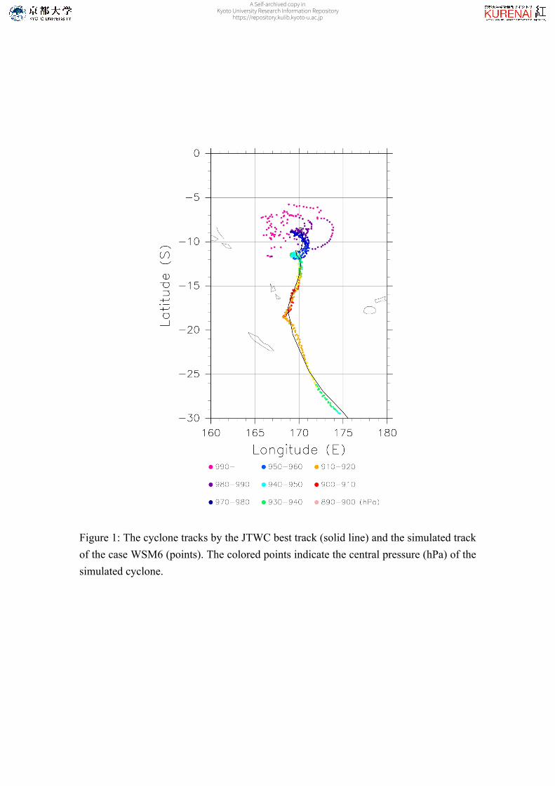
Figure 1: The cyclone tracks by the JTWC best track (solid line) and the simulated track of the case WSM6 (points). The colored points indicate the central pressure (hPa) of the simulated cyclone.



Figure 2: The time series of (a) maximum surface wind speed, (b) minimum surface central pressure and (c) radius of maximum surface wind speed in the simulations of WSM6 (red line), THOM (blue line), and MORR (green line). The black dots in (a) indicate the observed values from the JTWC best-track data.



Figure 3: The radar reflectivity (colored) and surface pressure (contoured) of the simulated tropical cyclone at 1200 UTC 12 March 2015 in Domain 2 of the WSM6 experiment.



Figure 4: The same as Fig. 3, except for at 0000 UTC 8 March 2015 in Domain 1.



(a) (b) (c)

Figure 5: The simulated radar reflectivity (color) and surface pressure (contoured) at 0000 UTC 7 March 2015 in the cases of (a) WSM6, (b) THOM, and (c) MORR.



(a) (b) (c)

Figure 6: The same as Fig. 5, except for at 0000 UTC 12 March 2015.



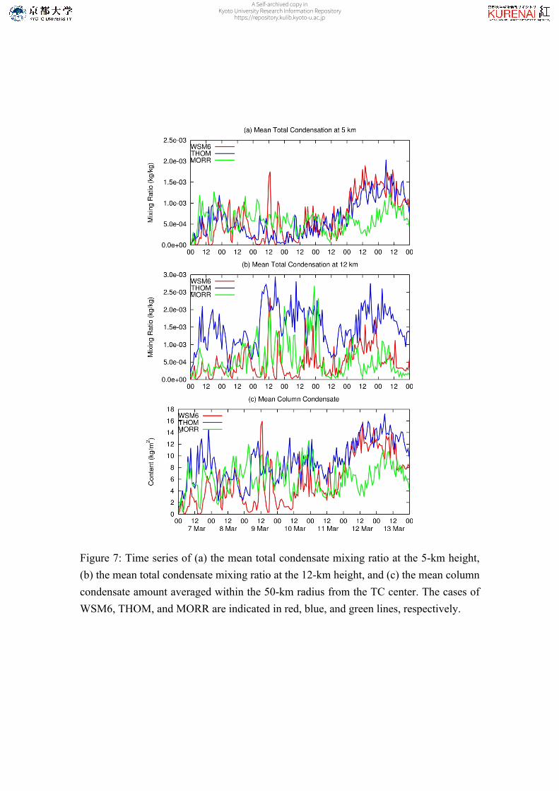
Figure 7: Time series of (a) the mean total condensate mixing ratio at the 5-km height, (b) the mean total condensate mixing ratio at the 12-km height, and (c) the mean column condensate amount averaged within the 50-km radius from the TC center. The cases of WSM6, THOM, and MORR are indicated in red, blue, and green lines, respectively.



Figure 8: Time series of the values of convective available potential energy (CAPE) computed within (a) the 500-km radius and (b) the 100-km radius from the TC center for the WSM6 (red line), the THOM (blue), and the MORR (green) cases.



(a) (b)

(c)

Figure 9: The maps of the maximum surface wind speed at each grid point during the simulated time period of Domain 2 for the cases of (a) WSM6, (b) THOM, and (c) MORR. The topography is contoured at the 200-m interval.



Table 1: The intensity of the simulated tropical cyclones in the three experiments.

ExperimentMinimum central

pressure (hPa)Maximum wind

speed (m s-1)Radius of maximum

wind speed (km)WSM6 903.6 66.2 39.6THOM 899.8 67.2 39.2MORR 911.8 59.6 45.8



title the evolution and intensification of cyclone pam

Documents