RIGHT:

URL:

CITATION:

AUTHOR(S):

ISSUE DATE:

TITLE:

Teaching Geometric Algebra withCLU$Calc$ (Innovative Teaching ofMathematics with GeometricAlgebra)

Perwass, Christian

Perwass, Christian. Teaching Geometric Algebra with CLU$Calc$(Innovative Teaching of Mathematics with Geometric Algebra).

2004-05

http://hdl.handle.net/2433/25644

33

Teaching Geometric Algebra with CLUCalc

University of Kiel, Cognitive Systems GroupChristian Perwass

Abstract

This text gives ashort overview of the features of the visualization software$CLUCa/c$, and how this software may be used to teach various aspects of GeometricAlgebra. CLUCafc is astand-alone software tool that uses the $3\mathrm{d}$-graphics libraryOpenGL to visualize the geometric meaning of elements of Geometric Algebras.These visualizations can very easily be animated or made user-interactive. Apartfrom this, Calc offers many more features like the annotation of graphics with$\mathrm{L}^{\mathrm{A}}\mathrm{I}\mathrm{E}\mathrm{X}$ text, the visualization of circle-valued functions, drawing of transparent okjects, user defined lighting, error propagation and much more.

1Introduction

Geometric Algebra (GA) has found its way into many areas of science, since DavidHestenes treated the subject in the ’

$60\mathrm{s}$ . Hestenes’ aim was in particular to find auni-fied language for mathematics, and he went about to show the advantages that couldbe gained by using GA in many areas of Physics and geometry [HS84, HZ91]. Manyother researchers followed and showed that applying GA in their field of research can beadvantageous, see $\mathrm{e}.\mathrm{g}$ . [LFLD98, PLO $\mathrm{I}$ , DorOl, LHROI].

However, since GA is usually not taught in high school or at universities, the subjectis not well known and seems mostly to be regarded as avery specialized and very difficultmathematical tool. This is the case even though many features of the algebra have adirect geometric interpretation and should thus lend themselves to simple explanations.One reason for this discrepancy may be that it is not always easy to imagine the geometricrelations, and for ateacher it is not easy to draw them.

In order to remedy this situation, Leo Dorst had developed aMatLab toolbox calledGABLE, which allowed the user to visualize GA elements in $3\mathrm{d}$-Euclidean space [DMBOO].Unfortunately, elements in projective or conformal space could not be visualized. Ithere-fore started in 2001 to develop a $\mathrm{C}++\mathrm{s}\mathrm{o}\mathrm{f}\mathrm{t}\mathrm{w}\mathrm{a}\mathrm{r}\mathrm{e}$library, which could automatically interpretelements of a GA in terms of their geometric representation and visualize them. This vi-sualization was done using the OpenGL $3\mathrm{d}$-graphics library and worked for $3\mathrm{d}$-Euclidean

数理解析研究所講究録 1378巻 2004年 33-50

34

space and the corresponding projective and conformal spaces. The software library, calledCLUDraw, was made available in August 2001 under the GNU Public License agreementas OpenSource software.

The drawback of this library was, that a user had to know how to program $C++\mathrm{i}\mathrm{n}$ orderto use it. Furthermore, every time the program was changed, it had to be $\mathrm{r}\mathrm{e}$-compiled inorder to visualize the new result. Many people that might have been interested GA couldtherefore not use this tool, and even for those who did know how to program in $C++$ , itwas quite tedious to constantly $\mathrm{r}\mathrm{e}$-compile a program when a small change was made toa variable.

I therefore decided to develop a stand-alone program, with an integrated parser, suchthat formulas could be typed in and visualized right away. This software, called CLUCalc, was first made available for download in February 2002. As of November 2003 it isavailable in version 3.0, including many advanced features like solving simple multivectorequations, error propagation calculations, text annotations using $L^{\mathrm{A}}\mathrm{I}ffl$ , and support for apresentation mode, which integrates interactive and animated $3\mathrm{d}$-graphics in presentationslides.

The basic philosophy behind CLXJCalc is that the user has a GA formula and wouldlike to know what this formula implies geometrically. I therefore developed the parser tobe used in CLVCalc from scratch. In this way I could choose the symbols representing thedifferent products in GA such that they are as close as possible to the ones used on paper.The resulting script language is called $CLUScr\dot{v}pt$ [Per03]. For example, the formula

$Y=(A\wedge B)\cdot$ $X$ becomes $\mathrm{Y}=(\mathrm{A}\wedge \mathrm{B})$ $\mathrm{X}$

when written in CLUScript In order to visualize the result of this calculation, $C\mathrm{L}UScr\dot{p}t$

defines the colon-0perator (:), such that $:Y=$ (A ” B) $\mathrm{X}$ visualizes $Y$ .In this text I will try to show the potential CLVCalc offers for teaching $\mathrm{G}\mathrm{A}$ , by demon-

strating different aspects of $\mathrm{G}\mathrm{A}$ . I will also demonstrate features of CLVCalc which haveno direct relation to $\mathrm{G}\mathrm{A}$ . This is to show that CLVCalc may also be used to teach othersubjects than $\mathrm{G}\mathrm{A}$ . In the following I will assume that the reader is familiar with thebasic concepts of $\mathrm{G}\mathrm{A}$ . An introduction to the fundamental aspects of GA can be found in[PH03], which includes an “interactive” introduction using CLUScript Mathematicallyrigorous and more in-depth introductions and discussions of GA (aka Clifford algebra)can be found, for example, in [HS84, Hes86, HZ91, GLD93, LOu97, Rie93, GM91, POr95,LFLD98, DorOl, PerOO, DMBOO]. The example scripts presented in the following will runwith CLUCafc 3.1, which may be downloaded from $\mathrm{w}\mathrm{w}\mathrm{w}$ . clucalc. $\mathrm{i}\mathrm{t}$ .

2 Using CLVCalc

In order to describe geometry, typically the Geometric Algebra of $3\mathrm{d}$-Euclidean space orthe corresponding projective and conformal spaces are considered. In each space vector$\mathrm{s}$

35

and blades usually represent different geometric entities and therefore have to be ana-lyzed differently. CLUCalc allows the user to work in all three spaces mentioned aboveconcurrently and to transfer vectors from any one space to any other. Here is an examplescript:

$7\mathrm{A}\mathrm{e}$ $=\mathrm{V}\mathrm{e}\mathrm{c}\mathrm{E}3$ (1 ,2,0); $//\mathrm{C}\mathrm{r}\mathrm{e}\mathrm{a}\mathrm{t}\mathrm{e}$ vector in E3 at position (1 ,2,0)$7\mathrm{A}\mathrm{p}$

$=\mathrm{V}\mathrm{e}\mathrm{c}\mathrm{P}3(\mathrm{A}\mathrm{e})$ ; // Embed vector Ae in projective space$7\mathrm{A}\mathrm{n}$ $=\mathrm{V}\mathrm{e}\mathrm{c}\mathrm{N}3(\mathrm{A}\mathrm{p})$ ; // Embed projective vector in confomal space

The question mark at the beginning of each line is an operator that prints the contentsof the element on its right in a text window. The output of the above script is

$\mathrm{A}\mathrm{e}=1^{\wedge}\mathrm{e}1+2^{\wedge}\mathrm{e}2$

$\mathrm{A}\mathrm{p}=1^{\wedge}\mathrm{e}1+2^{\wedge}\mathrm{e}2+1^{\wedge}\mathrm{e}4$

An $=1^{\wedge}\mathrm{e}1+2^{\wedge}\mathrm{e}2+2.5^{\wedge}\mathrm{e}+1^{\wedge}\mathrm{e}0$

In projective space the homogeneous dimension is denoted by $\mathrm{e}4$ . In conformal space $\mathrm{e}$

denotes $e_{\infty}$ and $\mathrm{e}0$ denotes $e_{o}$ . Moving between the different spaces is particularly usefulto show the different geometric interpretations of blades in the different space. However,note that blades cannot directly be transferred from one space to another. This has tobe done via the constituent vectors. Here is an example:

$\mathrm{A}\mathrm{e}=\mathrm{V}\mathrm{e}\mathrm{c}\mathrm{E}3$ (1 , 0,0); $//\mathrm{C}\mathrm{r}\mathrm{e}\mathrm{a}\mathrm{t}\mathrm{e}$ unit vector along x-directionBe $=\mathrm{V}\mathrm{e}\mathrm{c}\mathrm{E}3(0,1,0)j$ $//\mathrm{C}\mathrm{r}\mathrm{e}\mathrm{a}\mathrm{t}\mathrm{e}$ unit vector along y-direction

: Red; // Switch current color to red.$:\mathrm{A}\mathrm{e}^{\wedge}\mathrm{B}\mathrm{e}$ ; // Visualize the outer product of Ae and Be

: line; // Switch current color to line.$:\mathrm{V}\mathrm{e}\mathrm{c}\mathrm{P}3(\mathrm{A}\mathrm{e})\wedge \mathrm{V}\mathrm{e}\mathrm{c}\mathrm{P}3$ (Be) ; // Visualize the outer product of Ae and Be

$//\mathrm{w}\mathrm{h}\mathrm{e}\mathrm{n}$ embedded in projective space

: Greenj $//\mathrm{S}\mathrm{w}\mathrm{i}\mathrm{t}\mathrm{c}\mathrm{h}$ current color to green.: $\mathrm{V}\mathrm{e}\mathrm{c}\mathrm{N}3$ (Ae) $\sim \mathrm{V}\mathrm{e}\mathrm{c}\mathrm{N}3$ (Be) $j$ // Visualize the outer product of Ae and Be

$//\mathrm{w}\mathrm{h}\mathrm{e}\mathrm{n}$ embedded in confomal space

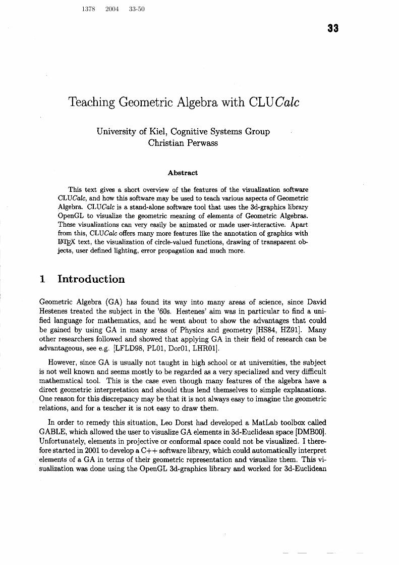
Note that the colon is an operator that tries to visualize the element on its right. TheLHS of figure 1 shows the resultant visualization of this script. The disc is the result of$\mathrm{A}\mathrm{e}^{\wedge}\mathrm{B}\mathrm{e}$ , the line the result of $\mathrm{V}\mathrm{e}\mathrm{c}\mathrm{P}3(\mathrm{A}\mathrm{e})^{\wedge}\mathrm{V}\mathrm{e}\mathrm{c}\mathrm{P}3$ (Be) and the two points are the result of$\mathrm{V}\mathrm{e}\mathrm{c}\mathrm{N}3$ (Ae) $\wedge \mathrm{V}\mathrm{e}\mathrm{c}\mathrm{N}3$ (Be). The disc represents the subspace spanned by Ae and Be, wherebythe area of the disc is the magnitude of the blade $\mathrm{A}\mathrm{e}^{\wedge}\mathrm{B}\mathrm{e}$ . In projective space the outerproduct of the embedded points $\mathrm{V}\mathrm{e}\mathrm{c}\mathrm{P}3$ (Ae) and $\mathrm{V}\mathrm{e}\mathrm{c}\mathrm{P}3$ (Be) represents the line passingthrough the points Ae and Be in Euclidean space. Hence, the representation as line. The

36

length of the line gives the magnitude of the corresponding blade. The outer product ofthe two vectors when embedded in conformal space ( $\mathrm{V}\mathrm{e}\mathrm{c}\mathrm{N}3$ (Ae) $\wedge \mathrm{V}\mathrm{e}\mathrm{c}\mathrm{N}3(\mathrm{B}\mathrm{e})$ ), representsthe point pair (Ae, Be) in Euclidean space and is visualized accordingly. Note that sucha point pair is in fact a one-dimensional sphere.

The RHS of figure 1 shows the same for the outer product of three vectors $a$ , $b$ and $c$ ,when regarded as Euclidean vectors and embedded in the corresponding projective andconformal space. The outer product of three Euclidean vectors in $3\mathrm{d}$-Euclidean space,represents the whole space. This is represented by the cube. The volume of the cube isequal to the magnitude of the blade. When these three vectors are embedded in projectivespace, their outer product represents a plane in Euclidean space, which is represented asa disc. Again, the area of the disc is the magnitude of the blade. The outer product of thethree vectors when embedded in conformal space represents a circle through these threepoints in Euclidean space. Hence, the circle drawn through the three points. The radiusof the circle can be extracted from the blade, but is not directly related to the magnitudeof the blade in conformal space.

Figure 1: The left image shows the geometric interpretation of the outer pr0-duct of two Euclidean vectors (the disc) and the geometric interpretation oftheir outer product when the vectors are embedded in the corresponding pr0-jective (the line) and conformal (the point pair) space. The right image showsthe same for three vectors. The Euclidean, projective and conformal interpre-tations are now the whole space, the disc and the circle, respectively.

Note that the script shown above does not automatically generate the annotations seenin figure 1. This has to be done with the help of additional commands as will be explainedlater on. Nonetheless, the images in figure 1 were generated directly with CLUCWc, andfor the annotations it is possible to use arbitrary ffIffl code

37

Intersections of geometric entities can also be evaluated and visualized quite easily.In GA the meet of two blades gives the blade representing the largest subspace the twoblades have in common. Geometrically speaking this is an intersection. In CLUCalcthe operator &is used to evaluate the meet of two multivectors. Note that when &isapplied to two integer values, it evaluates their bit-wise AND. In the following example

$\mathrm{s}\mathrm{c}\mathrm{r}\mathrm{i}\dot{\mathrm{p}}\mathrm{t}$ two spheres represented in conformal space are intersected and the resulting circleis intersected again with a plane.

SetPointSize (6); $//\mathrm{I}\mathrm{n}\mathrm{c}\mathrm{r}\mathrm{e}\mathrm{a}\mathrm{s}\mathrm{e}$ size of points for better visibilitySetLineWidth(4); // Increase width of lines for the same reason

$\mathrm{D}\mathrm{e}\mathrm{f}\mathrm{V}\mathrm{a}\mathrm{r}\mathrm{s}\mathrm{N}3()$ : // Define standard variables for confomal space: $\mathrm{N}3_{-}\mathrm{S}0\mathrm{L}\mathrm{I}\mathrm{D}://\mathrm{D}\mathrm{i}\mathrm{s}\mathrm{p}\mathrm{l}\mathrm{a}\mathrm{y}$ spheres as solid objects: DRAW-POINT-AS-SPHERE; $//\mathrm{D}\mathrm{r}\mathrm{a}\mathrm{w}$ points as small spheres and not as dots

// red green blue alpha $=\mathrm{t}\mathrm{r}\mathrm{a}\mathrm{n}\mathrm{s}\mathrm{p}\mathrm{a}\mathrm{r}\mathrm{e}\mathrm{n}\mathrm{c}\mathrm{y}$

: Color (1.000, 0. 378, 0.378, 0.8): $//\mathrm{U}\mathrm{s}\mathrm{e}$ a transparent color:Sl $=\mathrm{S}\mathrm{p}\mathrm{h}\mathrm{e}\mathrm{r}\mathrm{e}\mathrm{N}3(\mathrm{V}\mathrm{e}\mathrm{c}\mathrm{E}3(1), 1);//$ Make center of first sphere user-interactive

: MBlue; $//\mathrm{M}\mathrm{e}\mathrm{d}\mathrm{i}\mathrm{u}\mathrm{m}$ blue: $\mathrm{S}2=\mathrm{S}\mathrm{p}\mathrm{h}\mathrm{e}\mathrm{r}\mathrm{e}\mathrm{N}3$(0.5, 0, 0, 1); // Another sphere of radius $\mathrm{i}$

: Green;$:\mathrm{C}=$ Sl & S2; // The intersection of the two spheres

: Orange;// Create plane, whereby ’

$\mathrm{e}$’ is a predefined variable denoting

// the point at infinity. ’$\mathrm{e}$

’ is defined through the function// $\mathrm{D}\mathrm{e}\mathrm{f}\mathrm{V}\mathrm{a}\mathrm{r}\mathrm{s}\mathrm{N}3$ $()$ which was called in the fourth line.// The scalar factor only increases the size of $\mathrm{t}\mathrm{h}\mathrm{e}_{\wedge}\mathrm{p}1\mathrm{a}\mathrm{n}\mathrm{e}$

visualization.$:\mathrm{P}=10*\mathrm{V}\mathrm{e}\mathrm{c}\mathrm{N}3$(0,0. 0) $l$ .

$\mathrm{V}\mathrm{e}\mathrm{c}\mathrm{N}3(1,0,0)\Gamma\cdot \mathrm{V}\mathrm{e}\mathrm{c}\mathrm{N}3(0,0_{*}1)$ $\mathrm{e}$ ;

: Magent $\mathrm{a}$ ;: $\mathrm{X}$ $=\mathrm{P}$ & $\mathrm{C}_{1}$

. $//\mathrm{E}\mathrm{v}\mathrm{a}\mathrm{l}\mathrm{u}\mathrm{a}\mathrm{t}\mathrm{e}$ intersection of circle and plane

Figure 2 shows the result of the above script. Note that all intersections where evaluatedwith the same operation: the meet. The meet operator, as implemented in CLUCalc,regards only the algebraic properties of the multivectors and does know nothing abouttheir geometric interpretation. It is, in fact, a direct implementation of the mathematicaldefinition of the meet. The center of the sphere Sl in the above script, can be changedby the user interactively using the mouse. This will be explained in more detail in thenext section. If SI is moved by the user, such that the spheres do not actually intersectanymore, the meet operation returns an algebraic object that can be interpreted as a circlewith imaginary radius. This is also displayed by CLUCalc as a dotted circle. Imaginar

38

spheres and point pairs exist as well and are also visualized as transparent spheres andtwo points connected with a dotted line, respectively.

Typically one is also interested in visualizing functions. With CLUCalc scalar valued,vector valued and certain multivector valued functions can be drawn. One particularlyinteresting feature is the visualization of circle-valued functions. Since a circle can berepresented in conformal space as a trivector, i.e. the outer product of three vectors, thisis just a trivector valued function. The following script gives an example of this. Figure3 shows the visualization result of this script.

$\mathrm{D}\mathrm{e}\mathrm{f}\mathrm{V}\mathrm{a}\mathrm{r}\mathrm{s}\mathrm{N}3()$ $j//$ Define standard variables for confomal space$//\mathrm{C}\mathrm{r}\mathrm{e}\mathrm{a}\mathrm{t}\mathrm{e}$ a plane through points (0.0.1), (0.1.0)* (0,0,-1) and ’

$\mathrm{e}$’

$\mathrm{P}--\mathrm{V}\mathrm{e}\mathrm{c}\mathrm{N}3$(0.0 , 1) ..$\mathrm{V}\mathrm{e}\mathrm{c}\mathrm{N}3(0,1,0)$ $\wedge \mathrm{V}\mathrm{e}\mathrm{c}\mathrm{N}3(0,0 ,-1)\wedge \mathrm{e}j$

MyFunc – // This is how a function is defined{// Funct ion start

a $\cdot$ $-\mathrm{P}[1]$ ;// expect first parameter to be angle$\mathrm{b}=$ $-\mathrm{P}[21$ $j//\mathrm{e}\mathrm{x}\mathrm{p}\mathrm{e}\mathrm{c}\mathrm{t}$ second parameter to be radius$\mathrm{c}---\mathrm{P}[3]$ ; // expect third parameter to be $\mathrm{p}\mathrm{o}\mathrm{s}$ .$\mathrm{S}--\mathrm{S}\mathrm{p}\mathrm{h}\mathrm{e}\mathrm{r}\mathrm{e}\mathrm{N}3(0.0_{*}\mathrm{c}_{*}\mathrm{b});//\mathrm{c}\mathrm{r}\mathrm{e}\mathrm{a}\mathrm{t}\mathrm{e}$ a sphere$\mathrm{C}--\mathrm{S}$ &P; $//\mathrm{i}\mathrm{n}\mathrm{t}\mathrm{e}\mathrm{r}\mathrm{s}\mathrm{e}\mathrm{c}\mathrm{t}$ sphere with plane $\mathrm{P}$ which gives a circle$\mathrm{R}=\mathrm{R}\mathrm{o}\mathrm{t}\mathrm{o}\mathrm{r}\mathrm{N}3$ (0, 1.0, a) $j//\mathrm{c}\mathrm{r}\mathrm{e}\mathrm{a}\mathrm{t}\mathrm{e}$ a rotor.

$//\mathrm{N}\mathrm{o}\mathrm{w}$ rotate circle$(\mathrm{R}*\mathrm{C}*-\mathrm{R})//$ No semicolon here since this is the return value

$\}$ $//\mathrm{F}\mathrm{u}\mathrm{n}\mathrm{c}\mathrm{t}$ ion end

phi –0 $j$$//\mathrm{I}\mathrm{n}\mathrm{i}\mathrm{t}$ial angle value

Circle-list $–\mathrm{M}\mathrm{y}\mathrm{F}\mathrm{u}\mathrm{n}\mathrm{c}$ $(\mathrm{p}\mathrm{h}\mathrm{i}_{*}1,1)$ .$\cdot$ $//\mathrm{f}$ irst circleColor-list – Color (1 , 0,0); $//\mathrm{f}\mathrm{i}\mathrm{r}\mathrm{s}\mathrm{t}$ colorloop // start an infinite loop which needs to be stopped with ’break’$\{$

if (phi $>2*\mathrm{P}\mathrm{i}$ ) $//\mathrm{c}\mathrm{h}\mathrm{e}\mathrm{c}\mathrm{k}$ the loop-end conditionbreak $j$ // if satisf $\mathrm{i}\mathrm{e}\mathrm{d}$ , end loop.

$\mathrm{r}--$ pow $(\cos(1.5*\mathrm{p}\mathrm{h}\mathrm{i}), 2)+$ $0.1$ ;// make $\mathrm{r}$ a function of phi$\mathrm{d}--\mathrm{p}\mathrm{o}\mathrm{w}(\cos(1*\mathrm{p}\mathrm{h}\mathrm{i}), 2)$ $+0.1$ : $//\mathrm{m}\mathrm{a}\mathrm{k}\mathrm{e}$ $\mathrm{d}$ a function of phi

Circle.list $<<\mathrm{M}\mathrm{y}\mathrm{F}\mathrm{u}\mathrm{n}\mathrm{c}$ $(\mathrm{p}\mathrm{h}\mathrm{i}, \mathrm{r}, \mathrm{d})j//\mathrm{a}\mathrm{d}\mathrm{d}$ circle to list// Add corresponding color to list of colors$\mathrm{C}\mathrm{o}1\mathrm{o}\mathrm{r}_{-}1\mathrm{i}\mathrm{s}\mathrm{t}$ $<<\mathrm{C}\mathrm{o}1\mathrm{o}\mathrm{r}(\mathrm{r}-0.1. 0, 1. 1 - \mathrm{r})$ ;

phi $–\mathrm{p}\mathrm{h}\mathrm{i}$ $+\mathrm{P}\mathrm{i}/40.\cdot$ $//\mathrm{I}\mathrm{n}\mathrm{c}\mathrm{r}\mathrm{e}\mathrm{a}\mathrm{s}\mathrm{e}$ the value of phi$\}//\mathrm{J}\mathrm{u}\mathrm{m}\mathrm{p}$ to $\mathrm{s}\mathrm{t}$ art of loop

38

: Circle-list; $//\mathrm{V}\mathrm{i}\mathrm{s}\mathrm{u}\mathrm{a}\mathrm{l}\mathrm{i}\mathrm{z}\mathrm{e}$ the list of circles$//\mathrm{D}\mathrm{r}\mathrm{a}\mathrm{w}$ the surface over the circles using the corresponding colorsDrawCircleSurface (Circle-list, Color-list):

To make such surfaces look even better, it is also possible to add additional lights to thescene. Basically all lighting features offered by OpenGL can be accessed directly throughCLUCalc. For details on how to use lights, please refer to [Per03].

2.1 User Interaction

Although static visualizations of GA formulas are already quite useful, some propertiescan be understood much better with interactive visualizations. To make a visualizationuser-interactive is quite easily done with CLUCalc. For example, to generate a vectorthat can be changed by the user, one may simply write $\mathrm{V}\mathrm{e}\mathrm{c}\mathrm{E}3(1)$ . The number passedto the function $\mathrm{V}\mathrm{e}\mathrm{c}\mathrm{E}3$ denotes a so called ”mouse mod\"e. This mouse mode can be setvia a menu in CLUCalc. If, in this example, the user sets the mouse mode to 1, thenholds down the right mouse button and moves the mouse, the return value of $\mathrm{V}\mathrm{e}\mathrm{c}\mathrm{E}3(1)$

is changed and the whole script is $\mathrm{r}\mathrm{e}$-executed. Therefore, also anything that dependson the return value of $\mathrm{V}\mathrm{e}\mathrm{c}\mathrm{E}3(1)$ will be changed and $\mathrm{r}\mathrm{e}$-displayed. For more details onmouse modes see [Per03]. The scripts we presented so far may thus very easily be madeuser-interactive, simply by replacing the initial $\mathrm{V}\mathrm{e}\mathrm{c}\mathrm{E}3$ functions ffom fixed values (e.g.$\mathrm{V}\mathrm{e}\mathrm{c}\mathrm{E}3(1,0,0))$ , to mouse modes (e.g. $\mathrm{V}\mathrm{e}\mathrm{c}\mathrm{E}3(1)$ ).

Apart from generating user-interactive vectors, it is also possible to extract user-interactive scalar values which are related to certain mouse movements in given mous$\mathrm{e}$

40

modes. The function which does this is called Mouse. For example, the return value ofthe function call Mouse (1 , 2, 1) depends on the movement of the mouse along its x-axis,when mouse mode 1 is selected and the right mouse button pressed. The first parametergives the mouse mode, the second one the mouse button (1: left, 2: right) and the thirdparameter gives the axis (1: $x$ -axis, 2: $y$ -axis, 3: $z$ -axis). By default moving the mousewith the right mouse button pressed, changes the values for the $x$ and $z$ axes. When the“shift”-key is pressed at the same time, then the values for the $x$ and $y$ axes are changed.The Mouse-function for the left mouse button, i.e. second parameter set to 1, works verysimilar. The only difference is that the values returned lie in the range [0, $2\pi$ [. This isvery useful when making rotors interactive. Here is an example script.

// Use mouse mode 1 and left mouse button$7\mathrm{a}$ $=\mathrm{M}\mathrm{o}\mathrm{u}\mathrm{s}\mathrm{e}$ (1 , 1, 1); $//\mathrm{V}\mathrm{a}\mathrm{l}\mathrm{u}\mathrm{e}$ changed by movement in x-dir.$7\mathrm{b}$ $–$ Mouse (1 , 1, 2); $//\mathrm{V}\mathrm{a}\mathrm{l}\mathrm{u}\mathrm{e}$ changed by pressing “shift ”

$//\mathrm{a}\mathrm{n}\mathrm{d}$ moving in y-dir.$?\mathrm{c}$ $–$ Mouse(1, 1,3).$\cdot$

$//\mathrm{V}\mathrm{a}\mathrm{l}\mathrm{u}\mathrm{e}$ changed by NOT pressing $’\dagger \mathrm{s}\mathrm{h}\mathrm{i}\mathrm{f}\mathrm{t}^{11}$

$//\mathrm{a}\mathrm{n}\mathrm{d}$ movement in y-dir.

: Red; $//\mathrm{S}\mathrm{e}\mathrm{t}$ color to red: Ry $–\mathrm{R}\mathrm{o}\mathrm{t}\mathrm{o}\mathrm{r}\mathrm{E}3(0,1.0, \mathrm{a})$ : $//\mathrm{C}\mathrm{r}\mathrm{e}\mathrm{a}\mathrm{t}\mathrm{e}$ rotor about $\mathrm{y}$-axis with angle ’

$\mathrm{a}$’

: color . 1, 0.2. 0.8); $//\mathrm{S}\mathrm{e}\mathrm{t}$ color to given $(\mathrm{r}.\mathrm{g}.\mathrm{b})$ values:Rz – $\mathrm{R}\mathrm{o}\mathrm{t}\mathrm{o}\mathrm{r}\mathrm{E}3(0,0,1, \mathrm{b}).\cdot$ // Create rotor about z-axis with angle ’ $\mathrm{b}$ ’

: color(0.2, 0.8, 0. 1); $//\mathrm{S}\mathrm{e}\mathrm{t}$ color to given $(\mathrm{r},\mathrm{g}, \mathrm{b})$ values:Rx – $\mathrm{R}\mathrm{o}\mathrm{t}\mathrm{o}\mathrm{r}\mathrm{E}3$ $(1 ,0,0, \mathrm{c})$ ; // Create rotor about $\mathrm{x}$-axis with angle ’ c’

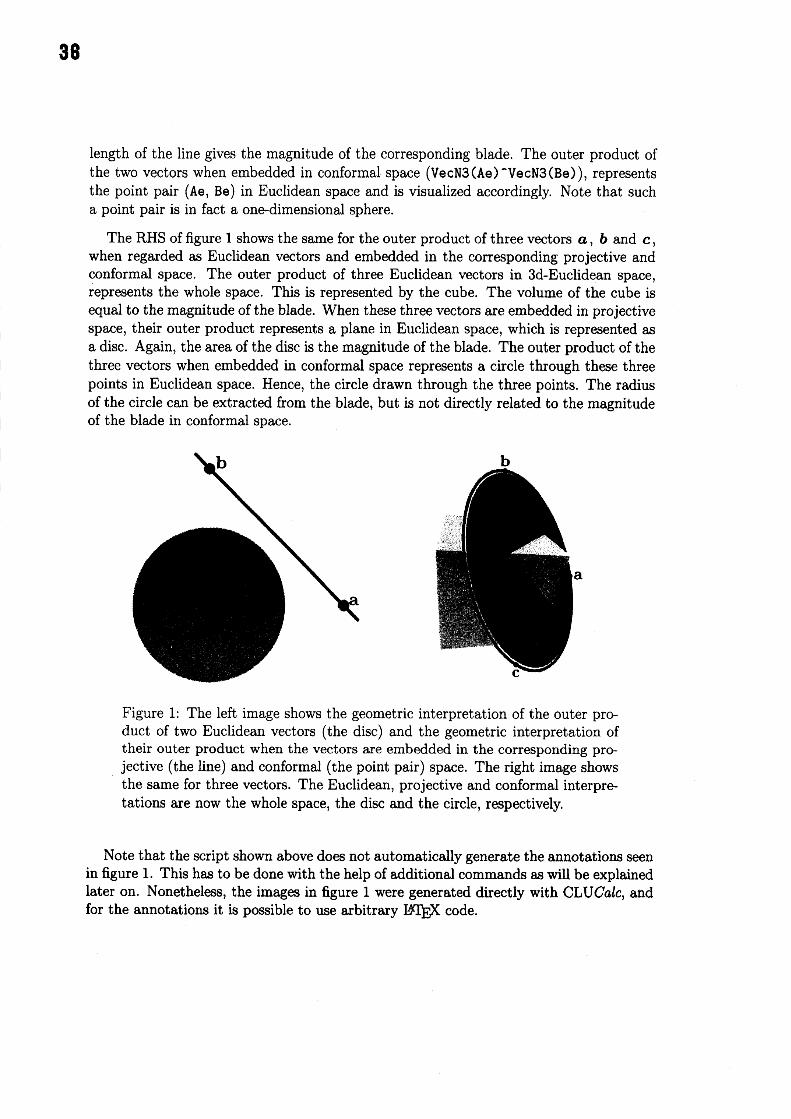
The text output window of CLUCalc will now display the values of $\mathrm{x}$ , $\mathrm{y}$ and $\mathrm{z}$ , andthe visualization window displays the rotors. Figure 4 shows an example visualization.A rotor is always visualized as a rotation axis with a partial disc perpendicular to it,representing the rotation plane and the rotation angle. By switching to mouse mode 1,holding down the left mouse button and moving the mouse, the visualization is changedcontinually, according to the mouse movement.

2.2 Animation

Apart ffom having user-interactive visualizations, it can be also very helpful to animatethem. Both features can also be mixed, such that the user can interact with some animatedfeatures. Again, it is very simply to animate a script with CLUCalc. First CLUCalc has tobe told that a script is to be animated. This is done with the script $\mathrm{l}\mathrm{i}\mathrm{n}\mathrm{e}-\mathrm{D}\mathrm{o}\mathrm{A}\mathrm{n}\mathrm{i}\mathrm{m}\mathrm{a}\mathrm{t}\mathrm{e}--1;$.Once the script is parsed, it is executed continually, with a maximum of 25 executionsper second. The number of executions that can be achieved per second, depends on thescript to be executed and the computer used

41

Figure 4: Three rotors about the $x$ , $y$ and -axes.

In order to generate animated visualizations, two variables are now available: Time anddTime. While the first gives the time in seconds elapsed since the start of the animation,the latter gives the elapsed time since the last execution of the script. Even though thetime variables give the time in seconds, their precision lies in the area of one millisecond.Here is an example script that uses animation.

$//\mathrm{E}\mathrm{n}\mathrm{a}\mathrm{b}\mathrm{l}\mathrm{e}$ animation of this script.JDoAnimate – 1 $i$

// Output time since start of animation in text output window.Time $j$

DegPerSec – 45; // Rotate with 45 degrees per second

$//\mathrm{E}\mathrm{v}\mathrm{a}\mathrm{l}\mathrm{u}\mathrm{a}\mathrm{t}\mathrm{e}$ current rotation angle. The variable ’RadPerDeg’// is predefined and gives radians per degree. The variable// ’Pi ’ is also predefined with the value of $\mathrm{p}\mathrm{i}$ .$//\mathrm{T}\mathrm{h}\mathrm{e}$ operator ’./,’ evaluates the modulus.Tangle $=$ (Time $*\mathrm{D}\mathrm{e}\mathrm{g}\mathrm{P}\mathrm{e}\mathrm{r}\mathrm{S}\mathrm{e}\mathrm{c}*\mathrm{R}\mathrm{a}\mathrm{d}\mathrm{P}\mathrm{e}\mathrm{r}\mathrm{D}\mathrm{e}\mathrm{g}$) $./$. $(2*\mathrm{P}\mathrm{i})j$

: Black $j$

// This will become the user-interactive rotation axis with// initial value (0, 1 , 0) , $\mathrm{i}.\mathrm{e}$ . the y-axis.: $\mathrm{w}--\mathrm{V}\mathrm{e}\mathrm{c}\mathrm{E}3(1)+\mathrm{V}\mathrm{e}\mathrm{c}\mathrm{E}3(0,1,0)$ ;

: Blue;

42

: $\mathrm{R}--\mathrm{R}o\mathrm{t}\mathrm{o}\mathrm{r}\mathrm{P}3$ ( $\mathrm{w}$ , angle); $//\mathrm{T}\mathrm{h}\mathrm{e}$ actual rotor about axis ’$\mathrm{w}$

’

: Red;$//\mathrm{T}\mathrm{h}\mathrm{e}$ plane through points (1.0, 0)

$\mathrm{f}$

$(1,1,0)\mathrm{f}$ $(1 ,0, 1)$ $\mathrm{f}$

$\mathrm{A}=\mathrm{V}\mathrm{e}\mathrm{c}\mathrm{P}3$ $(1,0,0)^{\wedge}\mathrm{V}\mathrm{e}\mathrm{c}\mathrm{P}3(1,1,0)^{\wedge}\mathrm{V}\mathrm{e}\mathrm{c}\mathrm{P}3(1,0 , 1)$ ;

$//\mathrm{T}\mathrm{h}\mathrm{e}$ plane A rotated $\mathrm{b}’ \mathrm{y}$ R. Note that $\sim \mathrm{R}$ denotes the reverse of R.: $\mathrm{B}--\mathrm{R}*\mathrm{A}*\sim \mathrm{R}.\cdot$

The animation feature may also be used to simulate physical effects like springs orgravitation. In this case it is usually necessary to initialize a set of variables during thefirst run of a script. Subsequent runs should then only adapt the variables’ current values.This can be done in CLXJCalc via the predefined variable ExecMode. The value of thisvariable may differ in each execution of a script and depends on the reason why the scriptwas executed. To check for a particular execution mode, a bit-wise AND operation ofExecMode with one of a set of predefined variables has to be done. For example, if thescript is executed because the user changed it, then ExecMode &EM-CHANGE is non-zero,where&is the operator for a bit-wise AND. This is used in the following example script,where a mass feels a gravitational pull towards the origin.

JDoAnimate – 1; $//\mathrm{M}\mathrm{a}\mathrm{k}\mathrm{e}$ this script animated

// Check whether script has just been loaded$//\mathrm{o}\mathrm{r}$ has been changed.if (ExecMode &EM-CHANGE)$\{$

// if true: intialize variables.TimeFactor –0.01; $//\mathrm{F}\mathrm{a}\mathrm{c}\mathrm{t}\mathrm{o}\mathrm{r}$ for simulation timestep$\mathrm{G}--6.67\mathrm{e}-2j$ $//$ Gravitational constant (in some units)

pos $–\mathrm{V}\mathrm{e}\mathrm{c}\mathrm{P}3(0,1_{*}0)$ ; $//\mathrm{P}\mathrm{o}\mathrm{s}\mathrm{i}\mathrm{t}\mathrm{i}\mathrm{o}\mathrm{n}$ vector in projective spacevel $–\mathrm{D}\mathrm{i}\mathrm{r}\mathrm{V}\mathrm{e}\mathrm{c}\mathrm{P}3(6,0.0)$ ; $//\mathrm{D}\mathrm{i}\mathrm{r}\mathrm{e}\mathrm{c}\mathrm{t}\mathrm{i}\mathrm{o}\mathrm{n}$ vector in projective space

Mass – 1; $//\mathrm{M}\mathrm{a}\mathrm{s}\mathrm{s}$ of object at origin0 $–\mathrm{V}\mathrm{e}\mathrm{c}\mathrm{P}3(0_{*}0,0)j//\mathrm{t}\mathrm{h}\mathrm{e}$ origin

$\}$

TdeltaT $=\mathrm{d}\mathrm{T}\mathrm{i}\mathrm{m}\mathrm{e}*\mathrm{T}\mathrm{i}\mathrm{m}\mathrm{e}\mathrm{F}\mathrm{a}\mathrm{c}\mathrm{t}\mathrm{o}\mathrm{r};//\mathrm{C}\mathrm{u}\mathrm{r}\mathrm{r}\mathrm{e}\mathrm{n}\mathrm{t}$ time step

dist – abs (pos -0); $//\mathrm{D}\mathrm{i}\mathrm{s}\mathrm{t}\mathrm{a}\mathrm{n}\mathrm{c}\mathrm{e}$ of mass to origindir – $(0 - \mathrm{p}\mathrm{o}\mathrm{s})/\mathrm{d}\mathrm{i}\mathrm{s}\mathrm{t}://\mathrm{N}\mathrm{o}\mathrm{m}\mathrm{a}\mathrm{l}\mathrm{i}\mathrm{z}\mathrm{e}\mathrm{d}$ direction to originacc $–\mathrm{G}*\mathrm{M}\mathrm{a}\mathrm{s}\mathrm{s}/$ (dist $*\mathrm{d}\mathrm{i}\mathrm{s}\mathrm{t}$ ; $//\mathrm{C}\mathrm{u}\mathrm{r}\mathrm{r}\mathrm{e}\mathrm{n}\mathrm{t}$ accelerationvel – vel $+\mathrm{a}\mathrm{c}\mathrm{c}*\mathrm{d}\mathrm{i}\mathrm{r}j//\mathrm{A}\mathrm{d}\mathrm{a}\mathrm{p}\mathrm{t}$ velocity

: Red;

43

:pos – pos $+\mathrm{v}\mathrm{e}\mathrm{l}*$ deltaT; $//\mathrm{A}\mathrm{d}\mathrm{a}\mathrm{p}\mathrm{t}$ position and draw it: Blue;: 0;

2.3 Annotating Graphics

It was mentioned above that it is possible to annotate graphics generated with CLUCalc using arbitrary fflIffl code. This is a very useful feature, because visualizations canbecome much more easy to understand when the different elements are labelled. Theadvantage of using $\mathrm{I}*\mathrm{I}\mathrm{f}\mathrm{f}\mathrm{l}$ code is clearly that virtually all mathematical symbols areavailable. It is also convenient for producing illustrations for printed texts, since the samesymbols can be used in the text and the illustration. In order for CLUCalc to be able torender BIffl code, the IATffi software environment and some other helper programs haveto be installed. For the exact details see [Per03].

In CLUCalc $\mathrm{I}4\mathrm{T}\Phi$ text can be rendered using the command DrawLatex. The text al-ways has to be drawn relative to a point. For example, to draw the text “Hello World” atposition (1, 1, 1), one can write DrawLatex (1, 1 , 1, “Hello World”. Instead of passinga string with the latex text, it is also possible to give a filename of a $I\mathit{4}Iffl$ file whichis rendered instead. The text is rendered as a bitmap and then drawn with the bot-tom left corner at the position given. Since the text is drawn as a bitmap, it is notchanged perspectively when moved around in the visualization space. It is also possibleto give an arbitrary adjustment of the text bitmap relative to the point given (see helpon SetLatexAlign in [Per03] $)$ .

The process of rendering a bitmap from PIffi code is not particularly fast. Therefore,rendered text bitmaps are cached, so they only have to be rendered once when the scriptis loaded. However, this would mean that anybody who wants use a script that containsIAIffl annotations must have $L^{\mathrm{A}}\mathrm{I}\mathrm{f}\mathrm{f}1$ installed. Furthermore, it can be quite annoying to al-ways wait for a couple of seconds before all the BIffi text for a script is rendered. For all ofthese reasons, the rendered IATffi bitmaps can be stored in files and are then readily avail-able when a script is loaded. For example, DrawLatex (1, 1, 1, “Hello World”, , ”textl)

renders the text “Hello World” and stores the rendered bitmap with a filename that isconstructed from the name of the script and “textl”. For more details on how to render$\mathrm{I}\mathrm{A}\mathrm{I}\mathbb{R}$ text see [Per03].

Apart from annotating geometric entities in a visualization, it is also practical to havetext that does not move with the visualization, as for example a title for the visualization.This is also possible with CLUCalc by drawing text in an overlay. Note that anything,not just text, can be drawn in an overlay, which allows for a static fore- or background.The following script gives an example of this feature. The corresponding visualization isshown in figure 5.

$\mathrm{D}\mathrm{e}\mathrm{f}\mathrm{V}\mathrm{a}\mathrm{r}\mathrm{s}\mathrm{E}3$ $()$ ; // Define variables for E3

44

$//\mathrm{S}\mathrm{e}\mathrm{t}$ Latex magnification. This is chosen very high here, since this// script was used to generate the corresponding figure for this text.SetLatexMagStep (20) ;SetPointSize (2); $//\mathrm{S}\mathrm{i}\mathrm{z}\mathrm{e}$ in which points are drawn:DRAW-POINT-AS-SPHERE; $//\mathrm{D}\mathrm{r}\mathrm{a}\mathrm{w}$ points not as dots but as small spheres: $\mathrm{E}3_{-}\mathrm{D}\mathrm{R}\mathrm{A}\mathrm{W}_{-}\mathrm{V}\mathrm{E}\mathrm{C}_{-}\mathrm{A}\mathrm{S}_{-}\mathrm{A}\mathrm{R}\mathrm{R}0\mathrm{W}$ : $//\mathrm{D}\mathrm{r}\mathrm{a}\mathrm{w}$ vectors in E3 as arrows.

:el :Red; // Draw basis vector el in red.: e2 : Green; // Draw basis vector e2 in green.: e3 : Blue; $//\mathrm{D}\mathrm{r}\mathrm{a}\mathrm{w}$ basis vector e3 in blue.

:Black; $//\mathrm{D}\mathrm{r}\mathrm{a}\mathrm{w}$ the following text in blackSetLatexAlignCO, 0.5); $//\mathrm{A}\mathrm{l}\mathrm{i}\mathrm{g}\mathrm{n}$ text $\mathrm{l}\mathrm{e}\mathrm{f}\mathrm{t}/\mathrm{c}\mathrm{e}\mathrm{n}\mathrm{t}\mathrm{e}\mathrm{r}\mathrm{e}\mathrm{d}$

DrawLatex (el , $|\mathrm{l}backslash \mathrm{v}\mathrm{e}\mathrm{c}\{\mathrm{e}\}_{-}1\^{\mathrm{t}\prime}$ . $||\mathrm{e}1’’$ ) $;//\mathrm{D}\mathrm{r}\mathrm{a}\mathrm{w}$ text

SetLatexAlign(0.5, 0); $//\mathrm{A}\mathrm{l}\mathrm{i}\mathrm{g}\mathrm{n}$ text $\mathrm{c}\mathrm{e}\mathrm{n}\mathrm{t}\mathrm{e}\mathrm{r}\mathrm{e}\mathrm{d}/\mathrm{b}\mathrm{o}\mathrm{t}\mathrm{t}\mathrm{o}\mathrm{m}$

DrawLatex (e2, $\prime\primebackslash \mathrm{v}\mathrm{e}\mathrm{c}\{\mathrm{e}\}_{-}2\’|$ , $\prime\prime \mathrm{e}2^{\mathrm{t}\prime}$ ) $://\mathrm{D}\mathrm{r}\mathrm{a}\mathrm{w}$ text

SetLatexAlign $\mathrm{C}1$ , 0. 5) ; $//\mathrm{A}\mathrm{l}\mathrm{i}\mathrm{g}\mathrm{n}$ text $\mathrm{r}\mathrm{i}\mathrm{g}\mathrm{h}\mathrm{t}/\mathrm{c}\mathrm{e}\mathrm{n}\mathrm{t}\mathrm{e}\mathrm{r}\mathrm{e}\mathrm{d}$

DrawLatex(e3. $\prime\primebackslash \mathrm{v}\mathrm{e}\mathrm{c}\{\mathrm{e}\}_{-}3\^{1\prime}$ , “e3’\dagger ); $//\mathrm{D}\mathrm{r}\mathrm{a}\mathrm{w}$ text

: $\mathrm{E}3_{-}\mathrm{D}\mathrm{R}\mathrm{A}\mathrm{W}_{-}\mathrm{V}\mathrm{E}\mathrm{C}_{-}\mathrm{A}\mathrm{S}$ -POINT; $//\mathrm{F}\mathrm{r}\mathrm{o}\mathrm{m}$ now on draw vectors again as points:Orange $j$

$//\mathrm{S}\mathrm{e}\mathrm{t}$ color to orange:A $–\mathrm{V}\mathrm{e}\mathrm{c}\mathrm{E}3(1)$ ; $//\mathrm{D}\mathrm{r}\mathrm{a}\mathrm{w}$ user-interactive vector: $\mathrm{B}\mathrm{l}\mathrm{a}\mathrm{c}\mathrm{k}_{1}$

. $//\mathrm{S}\mathrm{e}\mathrm{t}$ color to black for text drawingSetLatoxAlign (-0.05, 0) $i$ $//\mathrm{A}\mathrm{l}\mathrm{i}\mathrm{g}\mathrm{n}$ textDrawLatex ( $\mathrm{A}$ , $//\mathrm{D}\mathrm{r}\mathrm{a}\mathrm{w}$ fomula at position of ’A ’

$\mathrm{l}\downarrow\backslash [\backslash \mathrm{o}\mathrm{i}\mathrm{n}\mathrm{t}_{-}\{\backslash \mathrm{m}\mathrm{a}\mathrm{t}\mathrm{h}\mathrm{c}\mathrm{a}1\{\mathrm{S}\}\}\backslash ,$ $\mathrm{f}(\backslash \mathrm{v}\mathrm{e}\mathrm{c}\{\mathrm{x}\})\backslash ,$ $\mathrm{d}\backslash \mathrm{v}\mathrm{e}\mathrm{c}\{\mathrm{x}\}\backslash 1$ ”,$,|\mathrm{f}\mathrm{o}\mathrm{m}\mathrm{u}1\mathrm{a}’’)$ ;

StartOverlay $()$ : // Now start an overlay to draw text that does not move// when the user rotates or translates the above visualization.

SetLatexMagStep(26); $//\mathrm{I}\mathrm{n}\mathrm{c}\mathrm{r}\mathrm{e}\mathrm{a}\mathrm{s}\mathrm{e}$ size of Latex text renderingSetLatexAlign$(0, 1)$ ; $//\mathrm{A}\mathrm{l}\mathrm{i}\mathrm{g}\mathrm{n}$ text $\mathrm{l}\mathrm{e}\mathrm{f}\mathrm{t}/\mathrm{t}\mathrm{o}\mathrm{p}$ .DrawLatex(5, 5, 0, $’|\backslash \mathrm{s}1$ The Titl\"e, ’

$\mathrm{t}|\mathrm{t}\mathrm{i}\mathrm{t}\mathrm{l}\mathrm{e}’$); // Draw Title of slideEndOverlay $()$ ; $//\mathrm{E}\mathrm{n}\mathrm{d}$ overlay here

Together with the overlay feature, basically all prerequisites are available to give pre-sentations with CIAJCalc. Indeed, the other elements that are needed, like a full screenmode, stepping through a list of slides and using a white background, are also providedby $CLUCa/c$. In the $CLUCa/c$ distribution, an example presentation is included, whichcan serve as a template for your own presentations. Of course, preparing presentations in$CLUCa/c$ is not as easy as using a tool like StarOffice or PowerPoint, but CLXJCalc allowsyou to combine text with interactive $\mathrm{a}\mathrm{n}\mathrm{d}/\mathrm{o}\mathrm{r}$ animated $3\mathrm{d}$-graphics. For more details ongiving presentations with $CLUCa/c$, please see [Per03]

45

The Title

Figure 5: $\mathrm{I}4\mathrm{I}\mathrm{f}\mathrm{f}\mathrm{l}$ text in a visualization.

2.4 Multivector Calculations

Apart from the visualization features, CLUCalc also supports advanced calculations withmultivectors. A very useful operation is the inversion of a multivector, if the multivectorhas an inverse. The inversion is obtained with the ! operator. If a multivector has noinverse then zero is returned. For example, the script

$\mathrm{D}\mathrm{e}\mathrm{f}\mathrm{V}\mathrm{a}\mathrm{r}\mathrm{s}\mathrm{E}3$ $()$ $j$ // Define variables for E3

$?\mathrm{M}=1$ $+\mathrm{e}1$ $+\mathrm{e}2^{\wedge}\mathrm{e}3$ ; $//\mathrm{D}\mathrm{e}\mathrm{f}$ ine some multivector$7\mathrm{i}\mathrm{M}$ $–$ ! $\mathrm{M}$ ; $//\mathrm{E}\mathrm{v}\mathrm{a}\mathrm{l}\mathrm{u}\mathrm{a}\mathrm{t}\mathrm{e}$ inverse of $\mathrm{N}$

7’ $\mathrm{M}*\mathrm{i}\mathrm{M}$ – ” $+\mathrm{M}*\mathrm{i}\mathrm{M}$ ; // Check that $\mathrm{i}\mathrm{M}$ is inverse of $\mathrm{M}$

$7\mathrm{W}$ $–1+\mathrm{e}1i$ $//\mathrm{A}$ non-invertible multivector7 $\mathrm{i}\mathrm{W}=$ ! $\mathrm{W}$ ; $//\mathrm{T}\mathrm{h}\mathrm{e}$ inversion

results in the output

$\mathrm{M}=$ $1+1^{\wedge}\mathrm{e}1+1^{\wedge}\mathrm{e}23$

$\mathrm{i}\mathrm{M}$ $–0.2+0.2^{\wedge}\mathrm{e}1+-0.6^{\wedge}\mathrm{e}23+$ $0.4^{\wedge}$ I$\mathrm{M}*\mathrm{i}\mathrm{M}--1$

$\mathrm{W}--1$ $+1^{\wedge}\mathrm{e}1$

$\mathrm{i}\mathrm{W}$ $–0$

46

The inversion of multivectors offers the possibility to solve simple multivector equationsof the form $A$ $X=B$ for $X$ if $A$ and $B$ are known. More complex, linear equationscan be solved by regarding multivectors as simple vectors in a higher dimensional vectorspace, and GA products as bilinear functions in this space. $CLUCa/c$ supports this wayof looking at multivectors. The background to this functionality is the following.

The algebraic basis of a GA over a $n$ -dimensional vector space has dimension $2^{n}$ . If wedenote the algebraic basis of ($X(\mathbb{R}^{n})$ , i.e. the GA over the vector space $\mathbb{R}^{n}$ , by $\{E_{i}\}_{i=1}^{2^{n}}$ ,then an arbitrary multivector $A\in oe(\mathbb{R}^{n})$ can be written as

$A= \sum_{i=1}^{2^{n}}\alpha^{i}E_{i}$ ,

where the $\{\alpha^{i}\}_{i=1}^{2^{n}}\subset \mathbb{R}$ are scalars. The inner, outer and geometric product of GAbetween two multivectors may then be written as

$A \circ B=\sum_{i=1}^{2^{n}}\sum_{j=1}^{2^{n}}\sum_{k=1}^{2^{n}}\alpha^{i}\beta^{j}g_{ij}^{k}E_{k}$, (1)

where $B= \sum_{i=1}^{2^{n}}\beta^{i}E_{i}$ , $\circ$ is a placeholder for one of the products and $g_{i_{J}}^{k}$ is a tensorwhose entries are either 1, -1 or zero. This tensor encodes the particular properties ofthe product used. Therefore this tensor is different for each product. If a third multivector$C\in(\chi(\mathbb{R}^{n})$ is written as $C= \sum_{i=1}^{2^{n}}\gamma^{i}E_{i}$ and $C=A\circ B$ , then the relation between the$\{\alpha^{i}\}$ , $\{\beta^{J}\}$ and $\{\gamma^{k}\}$ follows from equation (1) as

$\gamma^{k}=\sum_{i=1}^{2^{n}}\sum_{j=1}^{2^{n}}\alpha^{i}\beta^{j}g_{ij}^{k}$. (2)

Now suppose $A$ and $C$ are known and $B$ is to be evaluated. This may be done by firstevaluating the sum over $i$ on the RHS, which then gives $\gamma^{k}=\sum_{j=1}^{2^{n}}\beta^{j}h_{j}^{k}$ , where $h_{j}^{k}:=$

$\sum_{i=1}^{2^{n}}\alpha^{i}g_{ij}^{k}$ . By writing the $\{\gamma^{k}\}$ and $\{\beta^{j}\}$ as column vectors $\mathrm{c}$ and $\mathrm{b}$ , respectively,and $h_{j}^{k}$ as matrix $\mathrm{H}$ , the above equation becomes $\mathrm{c}=\mathrm{H}\mathrm{b}$ , which may be solved for $\mathrm{b}$

by inverting H. This is exactly what is done by CLXJCalc internally, when the inverse ofa multivector is evaluated.

If instead of $A$ and $C$ , in the above example, $B$ and $C$ are known and $A$ is to beevaluated, then first the sum over $j$ has to be evaluated. Taking care of the order of theindices $i$ and $j$ of $g_{ij}^{k}$ is important, since the products are in general not commutative,i.e. $A\mathrm{o}B\neq B\mathrm{o}$ $A$ in general. In CLXJCalc the function GetMVProductMatrix is usedto evaluate the sum of the components of a multivector with the tensor $g_{ij}^{k}$ for a givenproduct. The functions $\mathrm{M}\mathrm{V}2\mathrm{M}\mathrm{a}\mathrm{t}\mathrm{r}\mathrm{i}\mathrm{x}$ and $\mathrm{M}\mathrm{a}\mathrm{t}\mathrm{r}\mathrm{i}\mathrm{x}2\mathrm{M}\mathrm{V}$ transform multivectors to a vectorrepresentation and vice versa. Here is a simple example script that evaluates the geometricproduct of two multivectors using this vector representation

47

$\mathrm{D}\mathrm{e}\mathrm{f}\mathrm{V}\mathrm{a}\mathrm{r}\mathrm{s}\mathrm{E}3$ $()$ ; // Define variables for E3A $–\mathrm{e}1$ ; $//\mathrm{D}\mathrm{e}\mathrm{f}\mathrm{i}\mathrm{n}\mathrm{e}$ multivector A$\mathrm{B}--\mathrm{e}2$ ; $//\mathrm{D}\mathrm{e}\mathrm{f}\mathrm{i}\mathrm{n}\mathrm{e}$ multivector $\mathrm{B}$

$//\mathrm{E}\mathrm{v}\mathrm{a}\mathrm{l}\mathrm{u}\mathrm{a}\mathrm{t}\mathrm{e}$ the matrix for the product A $*\mathrm{B}$ of the// components of A summed over index $\mathrm{i}$ of the$//\mathrm{t}\mathrm{e}\mathrm{n}\mathrm{s}\mathrm{o}\mathrm{r}\mathrm{g}^{\wedge}\mathrm{k}_{-}\mathrm{i}\mathrm{j}$ representing the geometric product.Agp $–\mathrm{G}\mathrm{e}\mathrm{t}\mathrm{M}\mathrm{V}\mathrm{P}\mathrm{r}\mathrm{o}\mathrm{d}\mathrm{u}\mathrm{c}\mathrm{t}\mathrm{M}\mathrm{a}\mathrm{t}\mathrm{r}\mathrm{i}\mathrm{x}$ ( $\mathrm{A}$ , MVOP.GP, 1 $/*\mathrm{f}\mathrm{r}\mathrm{o}\mathrm{m}$ left $*/$);

// Do the same for product $\mathrm{B}*$ A with components of a$\mathrm{g}\mathrm{p}\mathrm{A}--\mathrm{G}\mathrm{e}\mathrm{t}\mathrm{M}\mathrm{V}\mathrm{P}\mathrm{r}\mathrm{o}\mathrm{d}\mathrm{u}\mathrm{c}\mathrm{t}\mathrm{M}\mathrm{a}\mathrm{t}\mathrm{r}\mathrm{i}\mathrm{x}$ ( $\mathrm{A}$ , MVOP-GP, 0 $/*\mathrm{f}\mathrm{r}\mathrm{o}\mathrm{m}$ right $*/$ ) ;

// Transfom multivector $\mathrm{B}$ in matrix representation.$//\mathrm{B}\mathrm{m}$ is a column vector.Bm $–\mathrm{M}\mathrm{V}2\mathrm{M}\mathrm{a}\mathrm{t}\mathrm{r}\mathrm{i}\mathrm{x}(\mathrm{B})$ ;

$//\mathrm{T}\mathrm{h}\mathrm{e}$ operator $’*$ ’ between two matrices evaluated$//\mathrm{t}\mathrm{h}\mathrm{e}$ standard matrix product.Clm – Agp $*\mathrm{B}\mathrm{m}://\mathrm{E}\mathrm{v}\mathrm{a}\mathrm{l}\mathrm{u}\mathrm{a}\mathrm{t}\mathrm{e}$ A $*\mathrm{B}$

$\mathrm{C}2\mathrm{m}--\mathrm{g}\mathrm{p}\mathrm{A}*\mathrm{B}\mathrm{m};//\mathrm{E}\mathrm{v}\mathrm{a}\mathrm{l}\mathrm{u}\mathrm{a}\mathrm{t}\mathrm{e}\mathrm{B}*\mathrm{A}$

$7\mathrm{C}1$ $–\mathrm{M}\mathrm{a}\mathrm{t}\mathrm{r}\mathrm{i}\mathrm{x}2\mathrm{M}\mathrm{V}(\mathrm{C}\mathrm{l}\mathrm{m})$ ; // Transfom Clm back to a multivector$7\mathrm{C}2$ $–\mathrm{M}\mathrm{a}\mathrm{t}\mathrm{r}\mathrm{i}\mathrm{x}2\mathrm{M}\mathrm{V}(\mathrm{C}2\mathrm{m})$ ; $//\mathrm{T}\mathrm{r}\mathrm{a}\mathrm{n}\mathrm{s}\mathrm{f}\mathrm{o}\mathrm{m}$ $\mathrm{C}2\mathrm{m}$ back to a multivector

This script produced the text output

Cl – $1^{\wedge}\mathrm{e}12$

C2 $—1^{\wedge}\mathrm{e}12$

Many more things can be done with these functions. It is, for example, possible to mapnot a whole multivector to a vector, but only certain components. In this way, one can,for example, solve for a rotor numerically, while ensuring that the result can have onlyscalar and bivector components. For the details please refer to [Per03].

The matrices generated in the above script can also be visualized by CLUCalc. Forthis purpose the function Latex exists, which takes a matrix as parameter and returnsthe BIffl code that draws the corresponding matrix. The following code snippet can beadded to the end of the above script to draw the various matrices. The result of thisdrawing can be seen in figure 6. Not all details of this script can be explained here. Again[Per03] will be of help.

$-\mathrm{B}\mathrm{G}\mathrm{C}\mathrm{o}1\mathrm{o}\mathrm{r}$ $–\mathrm{W}\mathrm{h}\mathrm{i}\mathrm{t}\mathrm{e}$$j$ // Set Background color to White

$-\mathrm{F}\mathrm{r}\mathrm{a}\mathrm{m}\mathrm{e}\mathrm{B}\mathrm{o}\mathrm{x}\mathrm{S}\mathrm{i}\mathrm{z}\mathrm{e}=0$ ; // Do not draw a frame box

StartOverlay $()$$j$

$//\mathrm{S}\mathrm{t}$art an overla

46

SetLatexMagStep(14); // Increase Latex font size: Black: $//\mathrm{S}\mathrm{e}\mathrm{t}$ drawing color to blackSetLatexAlign $(0, 1)$ ; $//\mathrm{S}\mathrm{e}\mathrm{t}$ Latex aligment// The DrawLatex function returns a list of values that// give the extent of the rendered bitmap, so that more$//\mathrm{t}\mathrm{e}\mathrm{x}\mathrm{t}$ can be drawn next to it.Pl $–\mathrm{D}\mathrm{r}\mathrm{a}\mathrm{w}\mathrm{L}\mathrm{a}\mathrm{t}\mathrm{e}\mathrm{x}\mathrm{O}$ , 5, 0.

$\mathrm{l}|\backslash$ [ $\mathrm{A}\backslash \mathrm{c}\mathrm{i}\mathrm{r}\mathrm{c}--$\prime\prime

$+\mathrm{L}\mathrm{a}\mathrm{t}\mathrm{e}\mathrm{x}$ (Agp) $+’|\backslash$] $\mathfrak{l}1$ , $1\mathfrak{l}\mathrm{m}\mathrm{a}\mathrm{t}$ ’ $|$ ) $j$

$\mathrm{P}2=\mathrm{D}\mathrm{r}\mathrm{a}\mathrm{w}\mathrm{L}\mathrm{a}\mathrm{t}\mathrm{e}\mathrm{x}\mathrm{O}$ , Pl $[2]+5.0$ ,$\prime\prime\backslash$ [ $\backslash \mathrm{c}\mathrm{i}\mathrm{r}\mathrm{c}$ A $–\mathrm{t}\mathrm{t}+\mathrm{L}\mathrm{a}\mathrm{t}\mathrm{e}\mathrm{x}(\mathrm{g}\mathrm{p}\mathrm{A})+\mathrm{t}\mathfrak{l}\backslash$ ] $\prime \mathrm{l}$ , $\prime\prime \mathrm{m}\mathrm{a}\mathrm{t}2^{\prime 1})j$

DrawLatex ( $\mathrm{P}1[4]$ $+10_{*}5,0$ , $”\backslash [$ $\mathrm{B}\overline{-}’|+\mathrm{L}\mathrm{a}\mathrm{t}$ex (Bm) $+\prime\prime\backslash ]||$ . $’\uparrow \mathrm{b}^{\prime \mathrm{I}}$ ) :

DrawLatex (P2 $[4]$ +10* P2 [5]$t$

$0$ , $\prime\prime\backslash [$ C-l – ” $+\mathrm{L}\mathrm{a}\mathrm{t}\mathrm{e}\mathrm{x}$ (Clm) $+\prime\prime\backslash ]’|$ , lllc’) $j$

EndOverlay $()$ :

$A\mathrm{o}=(00000001$ $00000001$ $00000001$ $\frac{00000}{0,0’}1$ $00000001$ $\frac{000}{0000}1$ $00000001$ $00000001]$ $B=(\begin{array}{l}00\mathrm{l}00000\end{array}\}$

$oA$ $=(00000\mathrm{t}\mathrm{J}01$ $00000001$ $\frac{000000}{0}1$ $00000001$ $00000001$ $00000001$ $\frac{00}{00,000},1$ $00000001]$ $c_{1}=\{\begin{array}{l}000000\mathrm{l}0\end{array})$

Figure 6: Matrices drawn with $\mathrm{I}4\mathrm{W}$ in the visualization window.

Another advanced feature of CLVCalc is the evaluation of products in GA with errorpropagation. This means that for each multivector a covariance matrix can be definedrepresenting the uncertainty with which the multivector is known. It is then possible toevaluate the geometric, inner and outer product of multivectors with associated covariancematrices and propagate their uncertainties. Since intersections of geometric objects canin principle be evaluated using the inner, outer $\mathrm{a}\mathrm{n}\mathrm{d}/\mathrm{o}\mathrm{r}$ geometric product, it is possible todo uncertain geometric reasoning with CLVCalc. Furthermore, since in conformal spacecircles and spheres are represented in a linear fashion, error propagation extends readilyto these objects. One can, for example, evaluate the circle with associated covariance

43

matrix from three uncertain points, simply by evaluating their outer product with errorpropagation. Detail of how to use this functionality may again be found in [Per03].

3 Conclusions

The goal of this text was to give the reader a first impression of the features of CLUCalcand how they may be used for teaching geometry and subjects that profit from geometricvisualizations. I hope that the versatility of $CLUCa/c$, in terms of the different ways itmay be used, became clear.

1. CLUCalc is a tool that analyzes GA entities with respect to their geometric meaningand visualizes them. This can be very useful when learning about the GAs ofEuclidean, projective and conformal space, since students can play around with thedifferent entities and discover what the inner, outer and geometric product meangeometrically.

2. CLUCalc can be used to write scripts that evaluate complex algorithms, and offersa platform to easily visualize results as interactive $\mathrm{a}\mathrm{n}\mathrm{d}/\mathrm{o}\mathrm{r}$ animated $3\mathrm{d}$-graphics.This is certainly a useful aspect when doing research with $\mathrm{G}\mathrm{A}$ .

3. CLUCalc allows the user to produce images for printed publications, that use thesame BIffl fonts as the printed text. By allowing for transparent surfaces and userdefined lighting, the visual impact of $3\mathrm{d}$-graphics in a printed medium can also belargely increased.

4. All visualizations can be used right away in presentations. In particular, the com-bination of fixed text and interactive and animated $3\mathrm{d}$-graphics in a slide, furthersthe understanding of complex geometric relations and is also bound to catch theattention of an audience.

The whole software package is released as OpenSource software, to give students a cost-free tool that supports their studies, but also in the hope that a number of researchers bomthe GA community will join the development of CLUCalc and thus make it a powerfulplatform that furthers the research in $\mathrm{G}\mathrm{A}$ .

References

[DMBOO] Dorst L., MANN S., Bouma T.: GABLE: A MatLab tutorial for ge-ometric algebra. HTML document, 2000. Last visited 15. Sept. 2003,http: $//\mathrm{c}\mathrm{a}\mathrm{r}\mathrm{o}\mathrm{l}$ . wins. uva. $\mathrm{n}\mathrm{l}/\sim \mathrm{l}\mathrm{e}\mathrm{o}/\mathrm{G}\mathrm{A}\mathrm{B}\mathrm{L}\mathrm{E}/$ .

50

[DorOl] Dorst L.: Honing geometric algebra for its use in the computer sciences. In Ge0-metric Computing with Clifford Algebra (2001), Sommer G., (Ed.), Springer-Verlag,pp. 127-151.

[GLD93] GULL S. F., LASENBY A. N., DORAN C. J. L.: Imaginary numbers are not real-the geometric algebra of space time. Found. Phys. 23, 9 (1993), 1175.

[GM91] GILBERT J. E., MURRAY M. A. M.: Clifford algebra and Dime operators inhamonic analysis. Cambridge University Press, 1991.

[Hes86] HESTENES D.: New Foundations for Classical Mechanics. Dordrecht, 1986.

[HS84] HESTENES D., SOBCZYK G.: Clifford Algebra to Geometric Calculus: A UnifiedLanguage for Mathematics and Physics. Dordrecht, 1984.

[HZ91] HESTENES D., ZIEGLER R.: Projective Geometry with Clifford Algebra. ActaApplicandae Mathematicae 23 (1991), 25-63.

[LFLD98] LASENBY J. , FITZGERALD W. J., LASENBY A. , DORAN C.: New geometric methodsfor computer vision: An application to structure and motion estimation. InternationalJoumal of Computer Vision 3, 26 (1998), 191-213.

[LHROI] Ll H., HESTENES D., ROCKWOOD A.: Generalized homogeneous coordinates forcomputational geometry. In Geometric Computing with Clifford Algebra (2001), Som-mer G., (Ed.), Springer-Verlag, pp. 27-59.

[LOu97] LOUNESTO P.: Clifford Algebms and Spinors. Cambridge University Press, 1997.

[PerOO] PERWASS C : Applications of Geometric Algebra in Computer Vision. PhD thesis,Cambridge Universtiy, 2000.

[Per03] PERWASS C : The CLUScript online help. HTML document, 2003. Last visited 8.Feb. 2004, http: $//\mathrm{w}\mathrm{w}\mathrm{w}$ . perwass. $\mathrm{d}\mathrm{e}/\mathrm{C}\mathrm{L}\mathrm{U}/\mathrm{C}\mathrm{L}\mathrm{U}\mathrm{C}\mathrm{a}\mathrm{l}\mathrm{c}\mathrm{D}\mathrm{o}\mathrm{c}/$.

[PH03] PERWASS C, HILDENBRAND D.: Aspects of Geometr .c Algebra in Euclidean, Pm-jective and Conformal Space. Technical Report Number 0310, CAU Kiel, Institut f\"urInformatik und Praktische Mathematik, September 2003.

[PLOI] PERWASS C, LASENBY J.: A Unified Description of Multiple View Geometry. InGeometric Computing with Clifford Algebra (2001), Sommer G., (Ed.), Springer-Verlag.

[POr95] PORTEOUS I. R.: Clifford Algebras and the Classical Groups. Cambridge UniversityPress, 1995.

[Rie93] Riesz M.: Clifford Numbers and Spinors. Kluwer Academic Publishers, 1993