title reynolds equations for modeling the fluid flow and...

TitleA numerical study on differences in using Navier‒Stokes andReynolds equations for modeling the fluid flow and particletransport in single rock fractures with shear

Author(s) KOYAMA, T; NERETNIEKS, I; JING, L

Citation International Journal of Rock Mechanics and Mining Sciences(2008), 45(7): 1082-1101

Issue Date 2008-10

URL http://hdl.handle.net/2433/93463

Right

Copyright © 2007 Elsevier Ltd; この論文は出版社版でありません。引用の際には出版社版をご確認ご利用ください。This is not the published version. Please cite only thepublished version.

Type Journal Article

Textversion author

Kyoto University

A numerical study on differences in using Navier-Stokes or Reynolds

equations for simulating the fluid flow and particle transport in single rock

fractures with shear

T. Koyama1, I. Neretnieks2 and L. Jing1

1Engineering Geology and Geophysics Research Group, Department of Land and Water

Resources Engineering

2Division of Chemical Engineering, Department of Chemical Engineering and Technology

Royal Institute of Technology, KTH, S-100 44, Stockholm, Sweden

* Corresponding author. Tomofumi Koyama Engineering Geology and Geophysics Research Group, Department of Land and Water Resources Engineering, Royal Institute of Technology, KTH, S-100 44 Stockholm, Sweden. Tel.: +46-8-790 6807 Fax: +46-8-790 6810 E-mail address: [email protected] (T. Koyama) Submitted to Int J Rock Mech Min Sci on the 11th of May, 2007

- 1 -

mailto:[email protected]

Abstract The study on fluid flow and transport processes of rock fractures in most practical applications involves two fundamental issues: The validity of Reynolds equation for fluid flow (as most often assumed) and the effects of shear displacements on the magnitudes and anisotropy of the fluid flow velocity field. The reason for such concerns is that the impact of the surface roughness of rock fractures is still an unresolved challenging issue. The later has been systematically investigated with results showing that shear displacement plays a dominant role on evolutions of fluid velocity fields, for both magnitudes and anisotropy, but the former has not received examinations in details due to the numerical complexities involving solution of the Navier-Stokes (NS) equations and the representations of fracture geometry during shear. The objective of this paper aims to solve this problem through a FEM modeling effort. Applying the COMSOL Multiphysics code (FEM) and assuming a two-dimensional problem (for limitations in computational capacities and resources), we consider the coupled hydro-mechanical effect of fracture geometry change due to shear on fluid flow (velocity patterns) and particle transport (streamline/velocity dispersion), using measured topographical data of natural rock fracture surfaces. The fluid flow in the vertical 2-D cross-sections of single rock fractures was simulated by solving both NS and Reynolds equations, and the particle transport was predicted by the streamline particle tracking method with calculated flow velocity fields (vectors) from the flow simulations, obtaining results such as flow velocity profiles, total flow rates, particle travel time, breakthrough curves and the Péclet number, Pe, respectively. The results obtained using NS and Reynolds equations were compared to illustrate the degree of the validity of the Reynolds equation for general applications in practice since the later is mush more computationally efficient for large scale problems. The flow simulation results show that both the total flow rate and the flow velocity fields in a rough rock fracture predicted by NS equations were quite different from that as predicted by the Reynolds equation. The results show that a roughly 5-10 % overestimation on the flow rate is produced when the Reynolds equation is used, and the ideal parabolic velocity profiles defined by the local cubic law, when Reynolds equation is used, is no longer valid especially when the roughness feature of the fracture surfaces changes with shear. These deviations of flow rate and flow velocity profiles across the fracture aperture have a significant impact on the particle transport behavior and the associated properties, such as the travel time and Péclet number. The deviations increase with increasing flow velocity and become more significant when fracture aperture geometry changes with shear. Keywords: Rock fractures; fluid flow; particle transport; streamline/velocity dispersion; shear displacement; Navier-Stokes equation; Reynolds equation; Finite Element Method (FEM); particle tracking method.

- 2 -

1. Introduction The coupled processes of shear displacement, fluid flow and solute/particle transport processes in rock fractures are increasingly important research topics mainly due to the demands for design, construction, operation and performance/safety assessments of underground radioactive waste repositories and other civil and environmental engineering works such as underground storage caverns and oil/gas reservoir engineering. Fluid flow and solute/particle transport in rock fractures have been extensively studied experimentally, theoretically and numerically in the past [1-19] and comprehensive review works was reported in [20, 21]. However, the effects of shear on the fluid flow and transport phenomena in the fractures were not considered in these early works. Many laboratory studies on the effect of both normal stress and shear displacements on fluid flow through rock fractures, so-called coupled shear-flow tests, have been performed due to its importance to understand and quantify the coupled stress-flow processes in fractured rocks recently [22-28]. However, no coupled shear-flow-tracer tests have been performed under combined normal stress and shear displacements, even though the effect of the mechanical processes on the transport phenomena has been investigated by considering normal stresses without shear [29-31], shear displacement without normal stress [32] or with both shear displacement and normal stress [33], respectively. These recent studies represent a significant step forward in deepening our qualitative understanding of the hydro-mechanical and transport behaviour of rough rock fractures. In the above theoretical and experimental works, the validity of the cubic law is generally assumed, and further a mean value of the velocity of the ideal parabolic velocity profile across the fracture aperture, which is equal to 2/3 of maximum velocity of the parabolic profile according to the Reynolds equation, was generally used for the flow calculations. The Navier-Stokes (NS) equation is rarely applied in fluid flow analysis in fractures due to the numerical difficulties for its solution with complicated geometry of rock fractures, especially in 3D. When particle transport is concerned, the representation of the complete velocity profiles across the aperture, ideally parabolic or not, are required. This is due to the fact that the different flow velocities across the aperture cause different particle travel paths and times, which is well known as streamline/velocity dispersion [6, 10, 13, 19], and therefore affect the final evaluation of the particle transport behaviour and properties, such as break-through curves and Péclet number. Transport simulations are usually carried out using mean flow velocity calculated by flow simulation. Transport properties have been evaluated for single rock fractures as reported in [3-4, 11, 15, 30-32]. The validity of Reynolds equation and local cubic law are usually applied and the common understanding is that their applicability can be guaranteed only when the Reynolds number is very small (where viscous forces dominate the inertial forces) and aperture does not change abruptly [5, 9]. In reality, these requirements may not be met with rough rock fractures. The deviation of the flow velocity fields from ideal parabolic profiles across the fracture aperture, which could happen when fractures are not planar and smooth as required by Reynolds equation, could have a significant impact on the particle transport properties in rock fractures. The mechanical shear also plays important roles to change the geometry of fracture aperture and, therefore, give an additional increment on the geometric complexity of fracture apertures, resulting in additional complexities in the flow and transport properties of rock fractures. These issues can only be examined when direct solution of NS equations with detailed representation of roughness of fracture surfaces, with or without shear, is obtained. Needless to say, due to the geometric complexity, numerical solution techniques must be applied.

- 3 -

The objective of this paper is to examine the differences in simulating fluid flow behavior of rock fractures when more theoretically complete and sound NS equation and much simplified Reynolds equation were used, and their impacts on the studies of fracture geometry and its change during mechanical shear on the flow velocity fields/profiles and particle transport phenomena, especially streamline/velocity dispersion. The simulations have to be conducted numerically using 2-D cross-section geometry models of rock fractures, through the numerical solutions of the fluid flow by FEM. The comparison of the two sets of results then can be used to evaluate the degree of validity of the Reynolds equation for practical problems quantitatively. We assumed a steady state fluid flow through a vertical cross section of a rough fracture, due to the reason that full 3D representation of the rough fractures can only be accommodated by main-frame super computers and transport properties can be calculated for steady state flows in a straightforward fashion for more efficient comparison. 2. Methodology 2.1 Model setup A natural rock fracture surface, labeled as J1, was taken from the construction site of Omaru power plant in Miyazaki prefecture in Japan and used as the parent surface for creating fracture replicas for a series of coupled shear-flow tests under different normal constraint conditions and this study. The rock type is granite and the size of the specimen is 100 mm in width and 200 mm in length. The fracture surface J1 is very flat (JRC = 0-2) with very few major asperities on its surface. A three-dimensional laser scanning profilometer system with an accuracy of ±20 μm and a resolution of 10 μm was employed to obtain the topographical data of fracture surface, with an interval of 0.2 mm in both x and y-axes [28]. The results of coupled flow shear tests, assuming local validity of the cubic law and using mean flow velocity across the fracture aperture (the 2/3 of the maximum velocity of the ideal parabolic profile according to the Reynolds equation) with shear induced fluid velocity channeling and enhanced flow rate in the direction perpendicular to the shear direction are reported in the previous works [28, 33]. For generation of 2D geometric models of the rough fracture, one vertical cross section of the fracture sample J1 was selected in the middle of the sample as the lower profile of a fracture model, as shown in Fig. 1. Figure 2 shows how to create the 2D fracture models using this lower profile. The upper profile of the fracture model was created by a rigid-lifting of the lower profile for a vertical separation of 1.0 mm along the whole fracture length. To simulate shear, the lower profile is fixed and the upper one is translated in the –x-direction up to 2.0 mm, with a 1.0 mm shear displacement interval, and without any dilation, as shown in Fig.2a. At each shear displacement interval, aperture values along the fracture length was calculated in the direction perpendicular to the mean plane of the fracture model at 1000 measuring points. Along the fracture length, a (arithmetic) mean value of aperture over each 5 measuring points are calculated, thus the space between two rough profiles was modeled as an assemblage of 200 thin columns with an edge length of 1.0 mm (Fig.2b), distributed step-wise along the length of the fracture. The whole area of the fracture was divided into about 70,000 FEM elements for solving flow and transport problems. 2.2 Governing equations

- 4 -

The general description of fluid flow in a single fracture is given by the Navier-Stokes (NS) equations. In a steady state, the NS equations is expressed in a vector form as,

( ) p∇−∇=∇ uuu 2μρ , (1)

where ρ is the fluid density, μ is the fluid (dynamic) viscosity, u is flow velocity vector (u=(ux, uy, uz)), and p is the hydrodynamic pressure. Equation (1) is composed of a set of coupled nonlinear partial derivatives of varying orders. It is difficult and impractical to solve the Eq. (1) in closed-forms with very complicated geometry and under general boundary conditions, such as for flow through rough rock fractures. Therefore further simplifications are usually adopted for obtaining numerical solutions. The first level of simplification is to assume that inertial forces in the fluid are negligibly small compared with the viscous and pressure forces. Eq. (1) is then reduced to

, (2) p∇−∇= u20 μ

This equation is called the Stokes or ‘creeping flow’ equation. The Stokes equation has been solved numerically for rough fracture profiles and the validity of the simplification was examined in [7-8, 17]. However the use of Stokes equation for solving fluid flow problem in rock fractures is not common due mainly to its mathematical complexity. For the second level of simplification, some geometric and kinematic assumptions are necessary and the most common way is assuming the viscous flow under uniform pressure gradient between two smooth parallel plates. In this case, only one component of the flow velocity is nonzero and equations are much simplified, leading to the well-known Poiseuille flow with a parabolic velocity profile across the fracture aperture, b, defined by two parallel plates without roughness, with the fracture walls located at z=±b/2. The flow velocity fields are expressed as

⎥⎥⎦

⎤

⎢⎢⎣

⎡−⎟

⎠⎞

⎜⎝⎛

∂∂

−= 22

221 zb

xpux μ

, 0== zy uu . (3)

The total volumetric flow rate per unit width perpendicular to the direction of flow is then given by

pgbQx ∇−=μ

ρ12

3

, (4)

where b is the aperture of the idealized parallel smooth fracture. The term 123gbT ρ= is commonly called as the fracture transmissivity. Since transmissivity is proportional to the third power of the aperture, this relation is also called as the ‘cubic law’. In this case, the NS equation is reduced to the much simplified two-dimensional Reynolds equation by averaging in the aperture direction under the following kinematic and geometric constrains: the Reynolds number is very small (where viscous forces dominate the inertial forces) and aperture does not change abruptly [5, 9]. The Reynolds equation is expressed as

012

3

=⎟⎟⎠

⎞⎜⎜⎝

⎛∇⋅∇ pgb

μρ , (5)

Aperture-averaged models have been widely used for both fluid flow and solute transport simulations in rock fractures [5, 9]. The applicability of the aperture-averaged models/cubic law has also been discussed theoretically and numerically in [1-2, 5, 7-9, 17-18].

- 5 -

In this study, since a two-dimensional vertical cross section of a rough fracture was selected the aperture is no longer constant but varies along the fracture length. The unknown parameters in Eq. (1) include two components of flow velocity (in x- and z-directions, ux and uz,) and hydrodynamic pressure, p. Since Eq. (1) includes two equations for 2-D problems, one more equation is needed to solve for the three unknown parameters, ux, uz and p. The third equation is the continuity equation for incompressible Newtonian fluid and expressed as follows.

0=∇u (6)

To solve NS equations (Eq. (1)) together with continuity equation (Eq. (6)) for 2D problems, we used the commercial FEM software COMSOL Multiphysics [34]. The density and viscosity of water at 10°C were taken as 33109997.0 mkg×=ρ and , and the gravitational acceleration is taken as g =

sPa ⋅×= −310307.1μ2807.9 sm . We also solved Reynolds

equation (Eq. (5)) for the same flow problem assuming ideal parabolic velocity profile of ux, from column to column, so that differences between the results using two equations can be compared. Solving the Reynolds equation is then further simplified into a 1-D problem. Flow simulation results such as flow rates and flow velocity profiles across aperture are compared between results using the NS and Reynolds equations under different hydraulic pressures (as explained in the next section) and different shear displacements. 2.3 Boundary conditions The boundary conditions consist of: 1) no flow at the upper and lower fracture walls (profiles) representing impermeable rough rock surfaces; and 2) fixed hydraulic pressures at the inlet and outlet boundaries as shown in Fig. 3, with zero pressure at the outlet and pressure p=1 Pa, 10 Pa, 100 Pa and 1000 Pa, respectively, at the inlet (x=0). The hydraulic pressure 1 kPa is nearly equal to the 10 cm hydraulic head which was applied in the laboratory coupled shear-flow tests for single rock fractures in the previous works by the authors [28, 33]. It should be noted that since sample size becomes slightly shorter during the shear, pressure gradient through the fracture is not kept constant but becomes slightly larger. 2.4 Particle transport simulation – particle tracking method In this study, a Lagrangian approach using a particle tracking method was selected for particle transport simulations, considering only advection process. The random dispersion due to diffusion of the solute particles within the fluid in fractures and other retardation mechanisms such as diffusion, sorption or decay, were not taken into account. As the steady-state fluid flow was assumed, particle tracking along the streamlines was used. After solving the Navier-Stokes and Reynolds equations, flow velocity was calculated element by element and particles travel following the streamlines. It should be noted that particles are assumed to be massless in this study. For the particle injection at the inlet boundary, the number of particle injected at the elements along the inlet boundary is proportional to the element’s flow rates as defined by the velocity profile at the inlet [32], which was solved by using the pressure boundary condition while solving the NS equation. This means that more particles will be attracted to central or near central part of the fracture with higher flow velocities. Figure 4 shows the velocity profiles at the inlet boundary (without shear and hydraulic pressure is 1 kPa) and the number of the

- 6 -

particle injected is proportional to the flow rates for each section, which was calculated by multiplying flow velocity and section width. The location of particles injection is arranged regularly at an interval of 0.005 mm along the inlet boundary. This means that there are 199 injection points initially (1.0 mm fracture aperture before shear displacement applied). From the particle tracking simulations, travel time for each particle was obtained and can be evaluated for breakthrough curves, represented as the percentages of the particles collected at the outlet as functions of time. The Péclet number can be defined in terms of the variance and mean travel time using the following equation [35]

2

2 ⎟⎠⎞

⎜⎝⎛=

t

tPeσ

, (7)

where and 2tσ t are the variance and mean travel time, respectively. Pe is therefore a

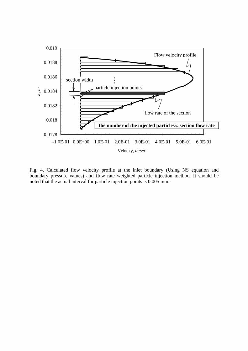
function of travel time t. 3. Results 3.1 Flow simulation results Figure 5 shows the evolution of flow velocity fields (absolute value of the flow velocity vector, |u|) and flow velocity profiles along three sections x=0.025-0.030 m (I), 0.095-0.10 m (II) and 0.155-0.160 m (III), for three different shear displacements of 0, 1 and 2 mm, and under two hydraulic pressures of 10 Pa (Fig. 5a, b, and c) and 1 kPa (5d, e, and f), respectively. In Zone I and III, the variation of the fracture geometry is large, defined by the waviness of the upper and lower profiles. Flow goes up first and down afterwards in Zone I but vice versa in Zone III, as shown by figures with cross-sectional velocity profiles. On the other hand, the variation of fracture geometry is small (smooth) in Zone II. The high-velocity paths are located close to the central part of the fracture. It can be seen that the velocity profiles are almost ideal parabolic when fluid flows through relatively smooth sections of fractures (e.g. Section II), but much distorted when with sudden change in aperture geometry occurs, as highlighted in zones I and III in Fig. 5. In order to compare more closely and clearly about the local behaviour of flow velocity profiles, the evolution of the flow velocity profiles (representing changes in both x and z-components of the flow velocity vectors, ux, and uz) during shear, and for different hydraulic pressures of 1 Pa, 10 Pa and 1 kPa are plotted at the several cross sections selected from each zone: x=0.025125, 0.026125 and 0.026875 m from Zone I, x=0.097125 m from Zone II and x=0.15725 and 0.158125 m from Zone III. The ideal velocity profiles as defined by the Reynolds equation (Eq. (5)) were also plotted as dotted curves without symbols, and are compared with the distorted ones predicted by simulations using the Navier-Stokes equations (the solid curves with symbols) in Fig. 6. The pattern of the fracture geometry change at each cross section during shear was also shown at the top of this figure, as enlarging, reducing (converging) or smoother transition. More clearly, with the results of NS solutions, the distortion of the flow velocities are shown in directions, shapes and magnitudes, compared with the ideal symmetric parabolic profiles using the parallel plate models (parabolic profiles of ux and zero uz, see also Eq. (3)) with the Reynolds equation results. The vertical z-components of the flow velocity vectors, uz are not zero generally (as will be the case with the use of the Reynolds equation) at selected cross sections and have positive or negative values depending on the flow going up (plus) or down (minus) vertically. The most

- 7 -

dramatic profile changes of uz occur when the fracture space becomes narrower or wider suddenly (sudden decreases of increases of apertures). The uz values change from positive to negative along the z-direction when the fracture space becomes narrower suddenly and the flow field converges (see Fig. 6b and c). On the other hand, when the fracture space becomes wider suddenly, the uz values change from negative to positive along the z-direction and the flow field diverges (see Fig. 6f). At x=0.097125 m in Zone II (Fig. 6d), the velocity profiles are close to ideal situation for all shear displacement stages with very small vertical velocity components. This is due to the fact that the fracture geometry is relatively smoother and does not change much during the shear. Even thought, small negative non-zero uz values are generated consistently since the continuous downward trend of the fracture in Section II (cf. Fig. 5). Several velocity profiles for the horizontal ux predicted by NS have flatter peaks (see Fig.6b, c and f), which indicates the formation of an inertial core between the walls. Negative values of the horizontal ux also occur in some sections (see Fig. 6b, c, e and f). This negative ux area appears when large rising up or lowering down of the fracture walls occur. This means that fluid flows backwards and rotates near the corners cause by such changes on the fracture walls, and the streamlines of that part become closed numerically. This rotational flow area appears more frequently when higher hydraulic pressure is applied with faster flow velocities. More discussion is given about this effect in the discussion section. Figure 7 shows the trajectories of maximum absolute flow velocity under different hydraulic pressures of 1, 10, 100 Pa and 1 kPa for different shear displacements of 0 and 2 mm, respectively. With the results using the Reynolds equation, the location of the maximum absolute flow velocity is always the central line (the dotted line) of the fracture space and the maximum velocity lines under different hydraulic pressure (the solid lines in color) using NS equation deviate from it, but the two sets of results are very close to each other. Certain deviation from the ideal situation occurs when fracture geometry changes suddenly as highlighted in Fig. 7 at a few local places but the overall agreement maintains in general. This may indicate that for the total flow rate the two sets of equations may yield matched results. The trajectory for low hydraulic pressure (therefore low velocity) follows the central line of the fracture and is more sensitive to the variation of the rough surface geometry. On the other hand, trajectory for higher hydraulic pressures does not follow the change of the fracture geometry exactly with sometimes shortcuts, as a results it becomes straighter and less tortuous. In this study, very large deviation of the trajectories of maximum absolute flow velocity from the center line, as reported in [12] for the high velocity flow (Re=52), was not observed even though our calculated maximum Reynolds number is about 200. The reason may be differences in the roughness of the walls. Figure 8a, b and c shows the total flow rates calculated by the two sets of the flow equations and ratios between them, Q_NS/Q_ideal, where Q_NS is the total flow rate by using the NS equations and Q_ideal is the total flow rate by using the Reynolds equation with ideal symmetric parabolic profile of ux, as functions of hydraulic pressure and Reynolds number for different shear displacements of 0, 1 and 2 mm, respectively. From Fig. 8a, there is no significant difference between the total flow rates calculated by using NS and Reynolds equations for all shear displacement cases and the relation between hydraulic pressures and flow rates varies linearly with hydraulic pressure, even though the total flow rate by the NS equation is always slightly smaller that that by the Reynolds equation. From Fig. 8b, the ratio Q_NS/Q_ideal is always smaller than 1.0 and becomes smaller with higher hydraulic pressures. The Q_NS/Q_ideal ratio is about 0.95 when applied hydraulic pressure is 1 Pa and decreases to 0.9 when applied pressure is 1 kPa. The comparison means that evaluated total flow rate by Reynolds equation (with assumed ideal parabolic flow velocity profiles or with averaged flow

- 8 -

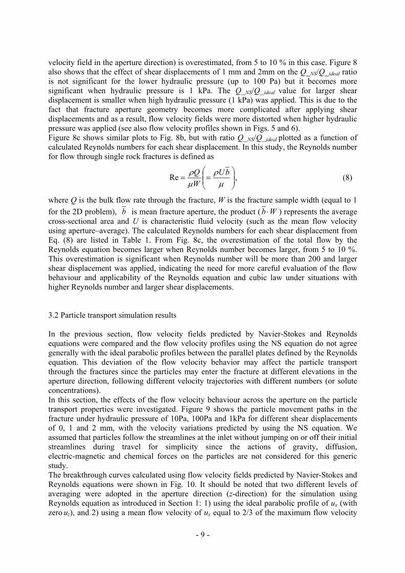
velocity field in the aperture direction) is overestimated, from 5 to 10 % in this case. Figure 8 also shows that the effect of shear displacements of 1 mm and 2mm on the Q_NS/Q_ideal ratio is not significant for the lower hydraulic pressure (up to 100 Pa) but it becomes more significant when hydraulic pressure is 1 kPa. The Q_NS/Q_ideal value for larger shear displacement is smaller when high hydraulic pressure (1 kPa) was applied. This is due to the fact that fracture aperture geometry becomes more complicated after applying shear displacements and as a result, flow velocity fields were more distorted when higher hydraulic pressure was applied (see also flow velocity profiles shown in Figs. 5 and 6). Figure 8c shows similar plots to Fig. 8b, but with ratio Q_NS/Q_ideal plotted as a function of calculated Reynolds numbers for each shear displacement. In this study, the Reynolds number for flow through single rock fractures is defined as

⎟⎟⎠

⎞⎜⎜⎝

⎛==

μρ

μρ bUWQRe , (8)

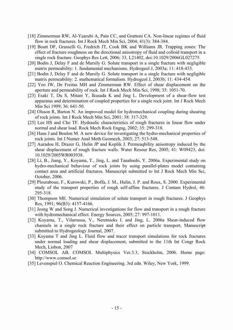
where Q is the bulk flow rate through the fracture, W is the fracture sample width (equal to 1 for the 2D problem), b is mean fracture aperture, the product ( Wb ⋅ ) represents the average cross-sectional area and U is characteristic fluid velocity (such as the mean flow velocity using aperture–average). The calculated Reynolds numbers for each shear displacement from Eq. (8) are listed in Table 1. From Fig. 8c, the overestimation of the total flow by the Reynolds equation becomes larger when Reynolds number becomes larger, from 5 to 10 %. This overestimation is significant when Reynolds number will be more than 200 and larger shear displacement was applied, indicating the need for more careful evaluation of the flow behaviour and applicability of the Reynolds equation and cubic law under situations with higher Reynolds number and larger shear displacements. 3.2 Particle transport simulation results In the previous section, flow velocity fields predicted by Navier-Stokes and Reynolds equations were compared and the flow velocity profiles using the NS equation do not agree generally with the ideal parabolic profiles between the parallel plates defined by the Reynolds equation. This deviation of the flow velocity behavior may affect the particle transport through the fractures since the particles may enter the fracture at different elevations in the aperture direction, following different velocity trajectories with different numbers (or solute concentrations). In this section, the effects of the flow velocity behaviour across the aperture on the particle transport properties were investigated. Figure 9 shows the particle movement paths in the fracture under hydraulic pressure of 10Pa, 100Pa and 1kPa for different shear displacements of 0, 1 and 2 mm, with the velocity variations predicted by using the NS equation. We assumed that particles follow the streamlines at the inlet without jumping on or off their initial streamlines during travel for simplicity since the actions of gravity, diffusion, electric-magnetic and chemical forces on the particles are not considered for this generic study. The breakthrough curves calculated using flow velocity fields predicted by Navier-Stokes and Reynolds equations were shown in Fig. 10. It should be noted that two different levels of averaging were adopted in the aperture direction (z-direction) for the simulation using Reynolds equation as introduced in Section 1: 1) using the ideal parabolic profile of ux (with zero uz), and 2) using a mean flow velocity of ux equal to 2/3 of the maximum flow velocity

- 9 -

predicted by the Reynolds equation, which was assigned to all elements along the aperture direction for each column, with uz=0. When the mean flow velocity option was adopted, particle travel time is identical for all particles across the fracture and all particles reach the outlet at the same time, which means that the shape of the breakthrough curves is a sharp stepwise function of time. When the velocity ux following ideal parabolic profiles of ux is used with Reynolds equation for flow simulations, the breakthrough curves are smooth curves with long tails due to the slow motions of particles near the wall. When the velocity fields predicted by NS equations were used, the breakthrough curves could not reach the 100 % level since some particles were trapped in the fracture and did not reach the outlet boundary, with two mechanisms: 1) some particles introduced too close to the walls with almost zero velocity so that they stay in the fracture; 2) some particles introduced near the fracture wall with small velocity but were trapped into rotational flow areas where fracture aperture changes suddenly (indicated by the negative values of the horizontal component of the flow velocity, ux (see Figs. 5 and 6). More detailed discussions about particle trapping zones are discussed in the next discussion section. The breakthrough curves using the NS flow solution is therefore truncated compared with that with Reynolds equation for flow simulations. The breakthrough curves calculated from velocity fields predicted by NS equations are always flatter than those calculated from the Reynolds equation, besides being truncated due to the loss of the trapped particles. They become flatter when higher hydraulic pressure was applied and flow velocity becomes faster. Since flatter breakthrough curves have larger dispersivity values, dispersion (streamline/velocity dispersion) becomes more significant when NS equation is used for the flow calculations. This is caused by the fact that disturbance to the flow velocity fields by the surface roughness of the fracture walls are more adequately represented in the NS equation and was ignored in the Reynolds equation. This effect will be more significant with increasing flow velocities (such as by increased hydraulic gradients). Table 2 shows the calculated mean and standard deviations of the particle travel time as functions of hydraulic pressure, using results by both NS and Reynolds (using the idealistic parabolic profile) equations at the identical percentage of particle collection at the outlet (since the truncated breakthrough curves using NS solutions). The mean travel time and standard deviation data are need to calculate the Péclet numbers characterizing the dispersion of the transport (cf. Eq. (7)), which is plotted in Fig. 11, corresponding to shear displacement of 0 mm, 1 mm and 2 mm, respectively. Since the NS solution generated trapping particles, it cannot be compared directly with the Reynolds equation results with 100% particle recovery. Therefore the Péclet numbers for both NS equation and Reynolds (with ideal parabolic profile) results were calculated at the same particle recovery percentage (cf. Fig. 10) defined by the NS solution, as shown in Fig. 11a for the Péclet number generated with NS solution and Fig. 11b for the Reynolds solution (with ideal parabolic profile of velocity). The Péclet numbers, Pe in Fig. 11, shows the similar evolution trend against applied hydraulic pressures, i.e. the Pe decreases with increasing applied hydraulic pressure, indicating increased dispersion. The effect of the shear displacements is not clear due to the fact that the shear displacement is small and dilation effects cannot be considered in 2D problems. It is important to note that the calculated Pe from the NS solution is always smaller than that using the Reynolds solution (with ideal parabolic velocity profiles). Since Péclet number, Pe and dispersivity, α has an inverse relation by definition ( αLPe = , where L is fracture length), the dispersivity is larger and streamline/velocity dispersion is more significant for the case using flow velocity fields predicted by NS equation. The effect of the streamline/velocity dispersion becomes more significant when the flow velocity becomes faster (smaller Pe for higher flow velocity).

- 10 -

4. Discussion and concluding remarks In this paper, the effect of fracture roughness and its change by shear on the flow velocity fields and particle transport behavior and properties (breakthrough curves and Péclet number) were investigated using 2-D cross-section models of rough rock fractures. The fluid flow was simulated by solving both the Navier-Stokes equations and its simplified form represented by the Reynolds equation, and particle transport was simulated by the streamline tracking method with flow velocity fields predicted by the solutions of the two sets of equations. The results obtained are the flow velocity profiles along the fracture length, total flow rates, particle travel time, breakthrough curves and the Péclet number, respectively. The flow simulation results show that the flow velocity fields predicted by NS equation were quite different from the ideal parabolic velocity fields defined by the local cubic law and Reynolds equation. This deviation gives a significant impact on the particle transport behavior and their properties. This deviation becomes larger especially when flow velocity becomes faster (or with higher pressure gradients). The mechanical shear plays important roles to change the fracture geometry, which, in turn, affects the flow and transport behaviour and properties of rock fractures. Besides the above general conclusions, a few specific scientific conclusions are drawn below. Currently, simplified models with different levels of geometric and physical representations using locally valid cubic law has been widely applied for the fluid flow simulations, and calculated mean flow velocity is often be used for transport simulations [3-4, 15, 30-33]. As shown by the results presented above, these simulations may be acceptable for total flow rate calculations with flow velocity fields averaged in the aperture direction, under appropriate hydraulic pressures and Reynolds numbers, but may not be suitable to simulate fluid flow behaviours without checking the suitable ranges of the Reynolds numbers and hydraulic gradients. A 5 to 10% overestimation of the total flow rate using the Reynolds equation may be acceptable for some applications as a conservative solution (such as safety assessment for nuclear waste repositories), but may be the opposite for others (such as geothermal energy extractions). It is especially important for laboratory experiments for coupled shear-flow processes to examine the test conditions in terms of hydraulic gradients and Reynolds numbers to ensure that the back calculated hydraulic apertures are reliable, preferably using the NS equation for the flow simulations, since the effects of the shear and hydraulic gradients affect the Reynolds number significantly. For particle transport simulations, the results from this study suggest that NS equation should be used for flow velocity simulations if the interactions between fracture surface and particles are needed, since adequate representation of the surface roughness is required in such cases. Such a study may not be practical for large scale applications, but detailed studies with representative fracture surface roughness features at representative fracture sizes can be investigated, based on experimental data, as the basis for extrapolation into the simplified large scale simulations. It may be especially needed for safety assessment of nuclear waste repositories where transport processes with more sophisticated particle retardation mechanisms requiring considerations for interactions between fracture surface, fluid and particles, electric-magnetic forces, and chemical reactions during the water-rock interactions. In addition to the above conclusions, a few outstanding issues involved in this paper are discussed in details below. a) Simplification from 3-D to 2-D problems

- 11 -

Although real flow and transport fields are much more complicated phenomena in 3-D and simulation model should be created in 3-D in theory at least, the 2-D vertical cross-section was selected as an analytical domain in this paper because the main purpose of this generic study is to investigate the effect of geometry roughness, and its change caused by mechanical shear, on the flow velocity and particle dispersion behaviors with the detailed representation of the velocity fields across the aperture direction inside a fracture, which has not been investigated in such details for rock fractures yet. The purpose of this approach is to examine how much difference in results is generated when simplified Reynolds equation is used instead of using the more complicated NS equations since solution of the later requires much more computational efforts. The drawback of using the simplified 2D vertical cross section model of rough rock fractures is that it cannot simulate large shear displacements and dilation due to the fact that larger shear displacement will cause contacts between the lower and upper surfaces of the fracture at some contacted asperities so that fluid flow is virtually blocked. This is the reason why two rough walls were separated by a 1.0 mm vertical gap initially to avoid any contact points during shear up to 2.0 mm. We also did not use any direct shear test data and do not consider any shear dilation since shear dilation at contact points were not present for open 2D fracture models as we considered here. This contact/dilation behavior can only be considered properly in 3D models with realistic rough surface representations since fluid flow bypassing contact areas can be simulated directly, as reported in [33]. However, numerical solution of NS equation for such 3D representations requires tremendous increase of computing power and resources that are not available to the authors at present. In any case, the 2D studies as presented in this paper can serve as generic example to detect quantitatively the theoretical differences in using NS and Reynolds equations. It needs to be noted that when fluid velocity field is predicted by using the Reynolds equation [3-4, 15, 30-33], the streamline/velocity dispersion behavior as we studied in this paper cannot be investigated since the flow velocity fields are averaged in the aperture direction. b) Validity of Reynolds equation and/or local cubic law The validity of Reynolds equation and/or local validity of the cubic law have been investigated extensively [1-2, 5, 7-9, 17-18]. From a theoretical study to investigate the validity of the cubic law though fractures with rough surfaces [1], it is concluded that a single-valued aperture cannot sufficiently characterize flow rates in rough fractures. Other physical and theoretical considerations such as the frequency distributions of apertures need to be incorporated into the cubic law. Some numerical experiments for solving Reynolds equation with a randomly generated fractal aperture distribution shows that surface roughness of natural rock fractures can cause a deviation from the cubic law prediction ranging from 10% to 50% [2]. The Reynolds equation was also employed to establish the analytical expressions of permeability dependency on the fracture roughness and mean aperture for sinusoidal fracture surfaces [5]. The results showed that the fracture surfaces should be smooth over the length of the order of one standard deviation of the fracture aperture in order for the Reynolds equation to be valid, and the associated errors will be considerable if the fracture surfaces become very rough [5]. The comparison of the predicted flow in idealized sinusoidal roughness fractures from using Reynolds equation with that from using the lattice-gas automaton method showed that the Reynolds equation overestimates the flow velocity when the surfaces are placed very closely together or the amplitude of the roughness increases relative to its wave length [7]. Stokes equation has been solved using the finite element technique and the results were compared with results from Reynolds equation [8, 17], with the conclusion that a simulation based on the Reynolds equation yields results with a reasonable validity. The difference in the evaluated mean hydraulic apertures obtained from

- 12 -

Stokes and Reynolds equations was about 2% [8]. The inertial effects will not be significant for flow at Reynolds number, Re, smaller than 1, where aperture is taken as the representative length scale for calculation of Re [9, 17]. In this study, the flow rates predicted by the Reynolds equation is always higher from 5 to 10 % than those predicted by the Navier-Stokes equation for the Reynolds number ranging from 0.2 to 200, which is similar to the results reported in [2, 7, 17]. c) The applicability of the particle tracking method The streamline particle tracking is applicable when advective transport is dominant over diffusion. The particle movement in aperture direction caused by diffusion, can be calculated from the following equation

xΔ

tDx w ⋅≈Δ (9) where Dw is diffusivity in water (=10-9 m2/s) and t is time. In the present study, from Table 2, the mean particle travel time for advective transport is about 500~600 sec, 50~60 sec, 5~6 sec and 0.5~0.6 sec when the hydraulic pressures of 1 Pa, 10 Pa, 100 Pa and 1 kPa were applied, respectively. From Eq. (9), the distances of particle movement caused by diffusion are 0.71~0.77 mm, 0.22~0.24 mm, 0.071~0.077 mm and 0.022~0.024 mm. Comparing initial fracture aperture of 1 mm, the particle movement caused by diffusion will be more significant when flow velocity is lower. d) Particle injection methods – the flow rate-weighted particle injection method In this paper, the flow rate-weighted particle injection method was used. This injection method is more realistic because higher flow rate attracts more particles along the inlet boundary. However, evenly distributed particle numbers along the inlet were also used in some literature without evaluating its effect on the evaluated transport properties, such as breakthrough curves, dispersivity and Péclet number [10, 14, 19]. This issue is extensively investigated in [32]. e) Particle trapping In this paper, the flow velocity fields predicted by using Navier-Stokes show negative values for the x-component of flow velocity vectors as shown in Figs. 5 and 6. This indicates that rotational flow was induced at some sharp corners of fracture where sudden change of fracture aperture geometry occurs. This is the so-called particle trapping zone in this paper, as shown in Fig. 12. In theory, if particles travel by strictly following the streamlines, they will not go into these trapping zones with closed streamlines that will not occur in reality. However, if particles jump between streamlines due to other physical and/or chemical processes such as molecular diffusion, such trapping might occur to reduce the particle travel speed and generate long tails in the breakthrough curves. A similar particle trapping phenomena was observed from the fluid flow and colloid transport simulations by coupled lattice-Bolztman discrete element method (LBDEM) [19]. In our results, closed streamlines were formed at some sharp corners on the fracture walls that generated these trapping zones, as shown in Fig.12, and this is more likely a numerical artifact due to sudden change of aperture geometry. This numerical artifact can be eliminated or reduced when more smooth representation of rough surfaces with much refined meshes is used. Acknowledgement

- 13 -

The authors thank the Swedish Nuclear Power Inspectorate (SKI) for the financial support for the first author’s Ph.D studies at Royal Institute of Technology (KTH), Stockholm, Sweden. The authors also thank Dr. Y. Jiang’s group at Nagasaki University, Nagasaki, Japan for supplying the fracture surface data. References [1] Neuzil CE and Tracy JV. Flow through fractures. Water Resour Res, 1981; 17(3):

191-199. [2] Brown SR. Fluid flow through rock joints: The effects of surface roughness. J Geophys

Res, 1987; 92(B2): 1337-1347. [3] Moreno L, Tsang YW, Tsang CF, Hale FV and Neretnieks I. Flow and tracer transport in

a single fracture: stochastic model and its relation to some field observations. Water Resour Res, 1988; 24(12): 2033-2048.

[4] Thompson ME and Brown SR. The effect of anisotropic surface roughness on flow and transport on fractures. J Geophys Res, 1991; 96(B13): 21,923-21,932.

[5] Zimmerman RW, Kumar S and Bodvarsson GS. Lubrication theory analysis of the permeability of rough-walled fractures. Int J Rock Mech Min Sci Geomech Abstr, 1991; 28 (4): 325-331.

[6] Koplik J, Ippolito I and Hulin JP. Tracer dispersion in rough channels: A two-dimensional numerical study, Phys Fluid A, 1993; 5(6): 1333-1343.

[7] Brown SR, Stockman HW and Reeves SJ. Applicability of the Reynolds equation for modeling fluid flow between rough surfaces. Geophys Res Lett, 1995; 22(18): 2537-3540.

[8] Mourzenko VV, Thovert JF and Adler PM. Permeability of a single fracture: Validity of the Reynolds equation. J Phys II France, 1995; 5: 465-482.

[9] Zimmerman RW and Bodvarsson GS. Hydraulic conductivity of rock fractures. Transp Porous Media, 1996; 23: 1-30.

[10] Grindrod P and Lee AJ. Colloid migration in symmetrical non-uniform fractures: particle tracking in three dimensions. J Contam Hydrol, 1997; 27: 157-175.

[11] Plouraboue F, Hulin JP, Roux S and Koplik J. Numerical study of geometrical dispersion in self-affine rough fractures, Phys. Rev. E, 1998; 58(3): 3334-3346.

[12] Skjetne E, Hansen A and Gudmundsson JS. High-velocity flow in a rough fracture. J Fluid Mech, 1999; 383: 1-28.

[13] Detwiler RL, Rajaram H and Glass RJ. Solute transport in variable-aperture fractures: an investigation of the relative importance of Taylor dispersion and macrodispersion. Water Resour Res, 2000; 36(7): 1611-1625.

[14] James SC and Chrysikopoulos CV. Transport of polydisperse colloids in a saturated fracture with spatially variable aperture, Water Resour Res, 2000; 36(6): 1457-1465.

[15] Detwiller R and Rajaram H. Nonaqueous-phase-liquid dissolution in variable-aperture fractures: Development of a depth-averaged computational model with comparison to physical experiment. Water Resour Res, 2001; 37(12): 3115-3129.

[16] Drazer G. and Koplik J. Transport in rough self-affine fractures, Phys Rev E, 2002, 66, 026303, doi:10.1103/PhysRevE. 66. 026303.

[17] Brush DJ and Thomson. Fluid flow in synthetic rough-walled fractures: Navier-Stokes, Stokes, and local cubic law simulations. Water Resour Res, 2003; 39(4), 1085, doi:10.1029/2002WR001346.

- 14 -

[18] Zimmerman RW, Al-Yaarubi A, Pain CC, and Grattoni CA. Non-linear regimes of fluid flow in rock fractures. Int J Rock Mech Min Sci, 2004; 41(3): 384-384.

[19] Boutt DF, Grasselli G, Fredrich JT, Cook BK and Williams JR. Trapping zones: The effect of fracture roughness on the directional anisotropy of fluid and colloid transport in a single rock fracture. Geophys Res Lett, 2006; 33, L21402, doi:10.1029/2006GL027275.

[20] Bodin J, Delay F and de Marsily G. Solute transport in a single fracture with negligible matrix permeability: 1. fundamental mechanisms. Hydrogeol J, 2003a; 11: 418-433.

[21] Bodin J, Delay F and de Marsily G. Solute transport in a single fracture with negligible matrix permeability: 2. mathematical formalism. Hydrogeol J, 2003b; 11: 434-454.

[22] Yeo IW, De Freitas MH and Zimmerman RW. Effect of shear displacement on the aperture and permeability of rock. Int J Rock Mech Min Sci, 1998; 35: 1051-70.

[23] Esaki T, Du S, Mitani Y, Ikusada K and Jing L. Development of a shear-flow test apparatus and determination of coupled properties for a single rock joint. Int J Rock Mech Min Sci 1999; 36: 641-50.

[24] Olsson R, Barton N. An improved model for hydromechanical coupling during shearing of rock joints. Int J Rock Mech Min Sci, 2001; 38: 317-329.

[25] Lee HS and Cho TF. Hydraulic characteristics of rough fractures in linear flow under normal and shear load. Rock Mech Rock Engng, 2002; 35: 299-318.

[26] Hans J and Boulon M. A new device for investigating the hydro-mechanical properties of rock joints. Int J Numer Anal Meth Geomech, 2003; 27: 513-548.

[27] Auradou H, Drazer G, Hulin JP and Koplik J. Permeaqbility anisotropy induced by the shear displacement of rough fracture walls. Water Resour Res, 2005; 41: W09423, doi: 10.1029/2005WR003938.

[28] Li, B., Jiang, Y., Koyama, T., Jing, L. and Tanabashi, Y. 2006a. Experimental study on hydro-mechanical behaviour of rock joints by using parallel-plates model containing contact area and artificial fractures. Manuscript submitted to Int J Rock Mech Min Sci, October, 2006.

[29] Plouraboue, F., Kurowski, P., Boffa, J. M., Hulin, J. P. and Roux, S. 2000. Experimental study of the transport properties of rough self-affine fractures. J Contam Hydrol, 46: 295-318.

[30] Thompson ME. Numerical simulation of solute transport in rough fractures. J Geophys Res, 1991; 96(B3): 4157-4166.

[31] Jeong W and Song J. Numerical investigations for flow and transport in a rough fracture with hydromechanical effect. Energy Sources, 2005; 27: 997-1011.

[32] Koyama, T., Vilarrassa, V., Neretnieks I. and Jing, L. 2006a Shear-induced flow channels in a single rock fracture and their effect on particle transport, Manuscript submitted to Hydrogeology Journal, 2007.

[33] Koyama T and Jing L. Fluid flow and tracer transport simulations for rock fractures under normal loading and shear displacement, submitted to the 11th Int Congr Rock Mech, Lisbon, 2007

[34] COMSOL AB. COMSOL Multiphysics Ver.3.3, Stockholm, 2006. Home page: http://www.comsol.se

[35] Levenspiel O. Chemical Reaction Engineering. 3rd edn. Wiley, New York, 1999.

- 15 -

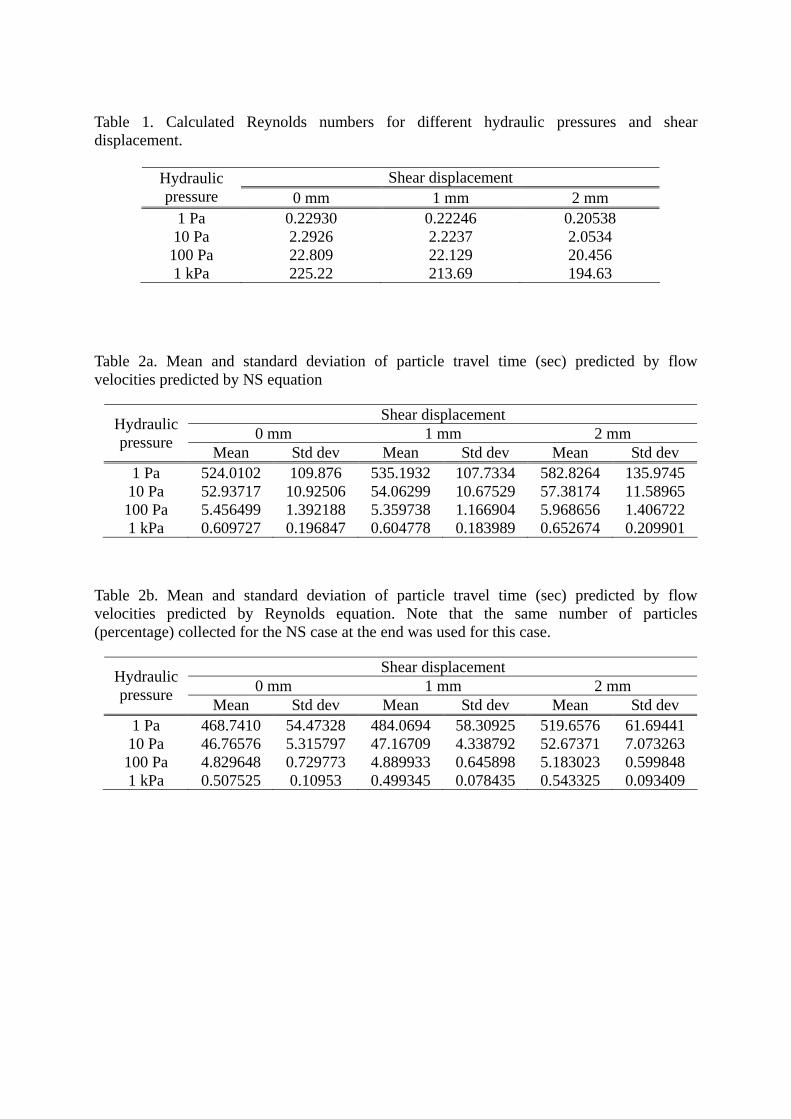
http://apps.isiknowledge.com/WoS/CIW.cgi?SID=Z27mPA813jofiIM3Fdh&Func=Abstract&doc=1/9

http://apps.isiknowledge.com/WoS/CIW.cgi?SID=Z27mPA813jofiIM3Fdh&Func=Abstract&doc=1/9

Table 1. Calculated Reynolds numbers for different hydraulic pressures and shear displacement.

Shear displacement Hydraulic pressure 0 mm 1 mm 2 mm

1 Pa 0.22930 0.22246 0.20538 10 Pa 2.2926 2.2237 2.0534 100 Pa 22.809 22.129 20.456 1 kPa 225.22 213.69 194.63

Table 2a. Mean and standard deviation of particle travel time (sec) predicted by flow velocities predicted by NS equation

Shear displacement 0 mm 1 mm 2 mm Hydraulic

pressure Mean Std dev Mean Std dev Mean Std dev 1 Pa 524.0102 109.876 535.1932 107.7334 582.8264 135.9745 10 Pa 52.93717 10.92506 54.06299 10.67529 57.38174 11.58965 100 Pa 5.456499 1.392188 5.359738 1.166904 5.968656 1.406722 1 kPa 0.609727 0.196847 0.604778 0.183989 0.652674 0.209901

Table 2b. Mean and standard deviation of particle travel time (sec) predicted by flow velocities predicted by Reynolds equation. Note that the same number of particles (percentage) collected for the NS case at the end was used for this case.

Shear displacement 0 mm 1 mm 2 mm Hydraulic

pressure Mean Std dev Mean Std dev Mean Std dev 1 Pa 468.7410 54.47328 484.0694 58.30925 519.6576 61.69441 10 Pa 46.76576 5.315797 47.16709 4.338792 52.67371 7.073263 100 Pa 4.829648 0.729773 4.889933 0.645898 5.183023 0.599848 1 kPa 0.507525 0.10953 0.499345 0.078435 0.543325 0.093409

x y z

(mm)

0 20 40 60 80 100 120 200 180 160 140 14

15

16

17

18

19

20

21 y=50 mm

Sample J1

z

a) b)

Fig. 1. a) 3-D topography of fracture surface specimen J1 (with a mesh size of 2 mm) and b) selected rough surface profile location at y=50 mm, with much magnified vertical scale.

b

Shear displacement

x

0.019

0.0185

0.018

0.0175

0.017

0 0.005 0.01 0.015 0.02 0.025 0.03

Shear direction

b= 1.0 mm

1.0 mm

a)

b)

z

Flow direction

Fig. 2. Model geometries of the 2D fracture. a) Parallel shift of the upper surface profile, with initial opening of 1.0 mm (b=1.0 mm), for simulating translational shear in the -x-direction, and b) Simplified geometry for numerical simulations using 200 thin columns with 1.0 mm width. Whole area was discretized with 70,000 triangle FEM elements.

Rough walls: No slip and no flow

Outlet: zero pressure, p=0

Flow direction

Inlet: constant pressures, p=pi (pi = 1, 10, 100 Pa and 1 kPa)

x

z

Fig. 3. Boundary conditions for fluid flow.

0.0178

0.018

0.0182

0.0184

0.0186

0.0188

0.019

-1.0E-01 0.0E+00 1.0E-01 2.0E-01 3.0E-01 4.0E-01 5.0E-01 6.0E-01

Velocity, m/sec

z, m

flow rate of the section

section width

Flow velocity profile

particle injection points

the number of the injected particles∝ section flow rate

Fig. 4. Calculated flow velocity profile at the inlet boundary (Using NS equation and boundary pressure values) and flow rate weighted particle injection method. It should be noted that the actual interval for particle injection points is 0.005 mm.

0 0.05 0.1 0.15 0.2

0.0165

0.016

0.0175

0.017

0.0185

0.018

0.019

Min: 0

Max: 5.798e-3

3

5

2

1

×10-3

0.0185

0.018

0.0175

0.017

0.0165 0.025 0.026 0.027 0.028 0.029 0.03

0.018

0.0175

0.017

0.0165 0.095 0.096 0.097 0.098 0.099 0.1

0.0185

0.018

0.0175

0.017

0.0165 0.155 0.156 0.157 0.158 0.159 0.16

0

4

I II III I

II

III

a)

0 0.05 0.1 0.15 0.2

0.0165

0.016

0.0175

0.017

0.0185

0.018

0.019

Min: 0

Max: 5.936e-3

3

5

2

1

×10-3

0.0185

0.018

0.0175

0.017

0.0165 0.025 0.026 0.027 0.028 0.029 0.03

0.018

0.0175

0.017

0.0165 0.095 0.096 0.097 0.098 0.099 0.1

0.0185

0.018

0.0175

0.017

0.0165 0.155 0.156 0.157 0.158 0.159 0.16

0

4

I

II

III

b)

0 0.05 0.1 0.15 0.2

0.0165

0.016

0.0175

0.017

0.0185

0.018

0.019

Min: 0

3

5

2

1

×10-30.0185

0.018

0.0175

0.017

0.0165 0.025 0.026 0.027 0.028 0.029 0.03

0.018

0.0175

0.017

0.0165 0.095 0.096 0.097 0.098 0.099 0.1

0.0185

0.018

0.0175

0.017

0.0165 0.155 0.156 0.157 0.158 0.159 0.16

0

4

6

Max: 6.031e-3

I

II

III

c)

Fig. 5. Evolutions of fluid flow velocity fields and cross-sectional profiles along sections x=25-30 (I), 95-100 (II) and 155-160 mm (III) under pi=10 Pa for shear displacements of a) 0 mm b) 1 mm and c) 2 mm, respectively. The values in the legend indicate the absolute flow velocity (unit: m/sec).

0 0.05 0.1 0.15 0.2

0.0165

0.016

0.0175

0.017

0.0185

0.018

0.019

Min: 0

0.5

0

0.4

0.3

0.2

0.1

0.0185

0.018

0.0175

0.017

0.0165 0.025 0.026 0.027 0.028 0.029 0.03

0.018

0.0175

0.017

0.0165 0.095 0.096 0.097 0.098 0.099 0.1

0.0185

0.018

0.0175

0.017

0.0165 0.155 0.156 0.157 0.158 0.159 0.16

Max: 0.576

I

II

III

d)

0 0.05 0.1 0.15 0.2

0.0165

0.016

0.0175

0.017

0.0185

0.018

0.019

Min: 0

0.5

0

0.4

0.3

0.25

0.2

0.0185

0.018

0.0175

0.017

0.0165 0.025 0.026 0.027 0.028 0.029 0.03

0.018

0.0175

0.017

0.0165 0.095 0.096 0.097 0.098 0.099 0.1

0.0185

0.018

0.0175

0.017

0.0165 0.155 0.156 0.157 0.158 0.159 0.16

Max: 0.524

0.45

0.35

0.15

0.1

0.05

I

II

III

e)

0 0.05 0.1 0.15 0.2

0.0165

0.016

0.0175

0.017

0.0185

0.018

0.019

Min: 0

0.5

0

0.4

0.3

0.25

0.2

0.0185

0.018

0.0175

0.017

0.0165 0.025 0.026 0.027 0.028 0.029 0.03

0.018

0.0175

0.017

0.0165 0.095 0.096 0.097 0.098 0.099 0.1

0.0185

0.018

0.0175

0.017

0.0165 0.155 0.156 0.157 0.158 0.159 0.16

Max: 0.533

0.45

0.35

0.15

0.1

0.05

I

II

III

f)

I II III

Fig. 5 (continued). Evolutions of velocity fields and cross-sectional profiles along sections x=25-30 (I), 95-100 (II) and 155-160 mm (III) under pi=1 kPa for shear displacements of d) 0 mm e) 1 mm and f) 2 mm, respectively. The values in the legend indicate the absolute flow velocity (unit: m/sec).

0.0170.01720.01740.01760.01780.018

0.01820.01840.0186

-2.0E-01 0.0E+00 2.0E-01 4.0E-01 6.0E-01Velocity, m/sec

z, m

0.01680.017

0.01720.01740.01760.01780.018

0.01820.01840.0186


z, m

0.0170.01720.01740.01760.01780.018

0.01820.01840.0186


z, m

0.01680.017

0.01720.01740.01760.01780.018

0.01820.01840.0186


z, m

0.0170.01720.01740.01760.01780.018

0.01820.01840.0186


z, m

0.01680.017

0.01720.01740.01760.0178

0.0180.01820.01840.0186


z, m

ux_0 mm uz _0 mm ux _1 mm uz _1 mm ux _2 mm uz _2 mm

ux _ideal uz _ideal

0 mm 1 mm 2 mm

x=0.025125

Flow direction

0 mm 1 mm 2 mm

x=0.026125

Flow direction

a) b)

1 Pa 1 Pa

10 Pa 10 Pa

1 kPa 1 kPa

Fig. 6. Evolutions of representative cross-sectional velocity profiles at a) x=0.025125 m and b) x=0.026125 m (from section I in the Fig. 5) under different pressures of 1 Pa, 10 Pa and1 kPa during shear displacements of 0 mm, 1 mm and 2 mm, for both horizontal and vertical velocity components, ux and uz, respectively.

0.01640.01660.01680.017

0.01720.01740.01760.0178


z, m

0.0170.01720.01740.01760.01780.018

0.01820.01840.0186


z, m

0.01640.01660.01680.017

0.01720.01740.01760.0178


z, m

0.0170.01720.01740.01760.01780.018

0.01820.01840.0186


z, m

0.01640.01660.0168

0.0170.01720.01740.01760.0178


z, m

0.0170.01720.01740.01760.0178

0.0180.01820.01840.0186


z, m

c) d)

0 mm 1 mm 2 mm

x=0.026875

Flow direction

1 Pa

10 Pa

1 kPa

0 mm 1 mm 2 mm

x=0.097125

Flow direction

1 Pa

10 Pa

1 kPa


ux _ideal uz _ideal

Fig. 6 (continued). Evolutions of cross-sectional velocity profiles at c) x=0.026875 m (from section I in the Fig. 5) and d) x=0.097125 m (from section II in the Fig. 5) under different pressures of 1 Pa, 10 Pa and1 kPa during shear displacements of 0 mm, 1mm and 2 mm, for both horizontal and vertical velocity components, ux and uz, respectively.

0.01640.01660.0168

0.0170.01720.01740.01760.0178

0.018


z, m

0.01660.0168

0.0170.01720.01740.01760.0178

0.018


z, m

0.01660.0168

0.0170.01720.01740.01760.0178

0.018


z, m

0 mm 1 mm 2 mm

x=0.15725

Flow direction

0 mm 1 mm 2 mm

x=0.0158125

Flow direction

e) f)


ux _ideal uz _ideal

0.01660.0168

0.0170.01720.01740.01760.0178

0.018


z, m

1 Pa

10 Pa

1 kPa

0.01640.01660.01680.017

0.01720.01740.01760.01780.018


z, m

0.01640.01660.0168

0.0170.01720.01740.01760.0178

0.018


z, m

1 kPa

10 Pa

1 Pa

Fig. 6 (continued). Evolutions of cross-sectional velocity profiles at e) x=0.026875 m and f) x=0.097125 m (from section III in the Fig. 5) under different pressures of 1 Pa, 10 Pa and1 kPa during shear displacements of 0 mm, 1mm and 2 mm, for both horizontal and vertical velocity components, ux and uz, respectively..

0.017

0.0175

0.018

0.0185

0.15 0.16 0.17 0.18x , m

y, m

0.017

0.0175

0.018

0.0185

0.07 0.08 0.09 0.1x , m

y, m

0.017

0.0175

0.018

0.0185

0.02 0.03 0.04 0.05x , m

z, m

0.017

0.0175

0.018

0.0185

0.15 0.16 0.17 0.18x , m

y, m

0.017

0.0175

0.018

0.0185

0.07 0.08 0.09 0.1x , m

y, m

0.017

0.0175

0.018

0.0185

0.02 0.03 0.04 0.05x , m

z, m

0.01550.016

0.01650.017

0.01750.018

0.01850.019

0.0195

0 0.02 0.04 0.06 0.08 0.1 0.12 0.14 0.16 0.18 0.2

x , m

z, m

wallwallidealP=1 PaP=10 PaP=100 PaP=1 kPa

0.01550.016

0.01650.017

0.01750.018

0.01850.019

0.0195

0 0.02 0.04 0.06 0.08 0.1 0.12 0.14 0.16 0.18 0.2

x , m

z, m

wallwallidealP=1 PaP=10 PaP=100 PaP=1 kPa

a)

b)

Fig. 7. Trajectories of the maximum absolute flow velocity under different hydraulic pressures of 1 Pa, 10 Pa, 100 Pa and 1 kPa for different shear displacements of a) 0 mm and b) 2 mm, using the Reynolds equation (the dashed line) and the NS-equation (the solid lines).

Fig. 8. Flow simulation results: a) comparison of the flow rates calculated from Navier-Stokes and Reynolds equations for different shear displacements, b) calculated ratio of flow rates using NS equation (QNS) and Reynolds equation (Qideal), QNS/Qideal, as a function of hydraulic pressure and c) calculated ratio of flow rates (QNS/Qideal) as a function of Reynolds number.

0.8

0.85

0.9

0.95

1

1.0E-01 1.0E+00 1.0E+01 1.0E+02 1.0E+03 1.0E+04

Hydraulic pressure, Pa

Q_N

S/Q

_ide

al

0 mm1 mm2 mm

a)

b)

1.0E-07

1.0E-06

1.0E-05

1.0E-04

1.0E-01 1.0E+00 1.0E+01 1.0E+02 1.0E+03 1.0E+04


Flow

rate

, m3 /s

ec

1.0E-03

Q_0mm_NSQ_0mm_idealQ_1mm_NSQ_1mm_idealQ_2mm_NSQ_2mm_ideal

0.8

0.85

0.9

0.95

1

1.0E-01 1.0E+00 1.0E+01 1.0E+02 1.0E+03Reynolds number, Re

Q_N

S/Q

_ide

al

0 mm1 mm2 mm

c)

0 0.05 0.1 0.15 0.2

0.0165

0.016

0.0175

0.017

0.0185

0.018

0.019

Min: 0

Max: 5.798e-3

3

5

2

1

0

4

0 0.05 0.1 0.15 0.2

0.0165

0.016

0.0175

0.017

0.0185

0.018

0.019

Min: 0

Max: 0.0564

0.05

0

0.04

0.03

0.02

0.01

0 0.05 0.1 0.15 0.2

0.0165

0.016

0.0175

0.017

0.0185

0.018

0.019

Min: 0

0.5

0

0.4

0.3

0.2

0.1

Max: 0.576

Min: 0

Max: 5.936e-3

3

5

2

1

×10-3

0

4

Min: 0

0.05

0

0.04

0.03

0.02

0.01

Max: 0.0581

Min: 0

0.5

0

0.4

0.3

0.25

0.2

Max: 0.524

0.45

0.35

0.15

0.1

0.05

a) b)

Pi=1 kPa

Pi=100 Pa

Pi=10 Pa

×10-3Max: 6.031e-3

6

Fig. 9. Particle motion trajectories with evolutions of velocity fields under hydraulic pressure of 10Pa, 100Pa and 1kPa with shear displacement of a) 0 mm b) 1mm and c) 2mm, respectively. The values in the legend indicate the absolute flow velocity (unit: m/sec).

Min: 0

3

5

2

1

0

4

Min: 0

Max: 0.0593

0.05

0

0.04

0.03

0.02

0.01

Min: 0

0.5

0

0.4

0.3

0.25

0.2

0.45

0.35

0.15

0.1

0.05

Max: 0.533

c)

Fig. 10. Breakthrough curves using flow velocities profiles predicted by Navier-Stokes and Reynolds equations (with ideal parabolic velocity profiles and the mean flow velocity) for differentshear displacement of a) 0 mm, b) 1 mm and c) 2 mm. It should be noted that mean flow velocity is 2/3 of the maximum flow velocity for the Reynolds equation case.

0102030405060708090

100

1.0E-01 1.0E+00 1.0E+01 1.0E+02 1.0E+03 1.0E+04

Time, sec

Parti

cles

, %

10 Pa 100 Pa 1 kPa

NS

1 Pa

parabolic

mean

Parabolic

NS mean

0102030405060708090

100

1.0E-01 1.0E+00 1.0E+01 1.0E+02 1.0E+03 1.0E+04

Time, sec

Parti

cles

, %

0102030405060708090

100

1.0E-01 1.0E+00 1.0E+01 1.0E+02 1.0E+03 1.0E+04

Time, sec

Parti

cles

, %

a)

b)

c)

10

20

30

40

50

60

1.0E-01 1.0E+00 1.0E+01 1.0E+02 1.0E+03 1.0E+04


Pe

Pe_0mmPe_1mmPe_2mm

0

50

100

150

200

250

1.0E-01 1.0E+00 1.0E+01 1.0E+02 1.0E+03 1.0E+04


Pe

Pe_0mm_idealPe_1mm_idealPe_2mm_ideal

a)

b)

Fig.11. Calculated Péclet number, Pe by Eq. (7), using a) flow velocities predicted by NS equation and b) flow velocities using Reynolds equation with ideal parabolic velocity profiles. Note that the same number of particles (percentage) which was collected for the NS case at the end was used for both cases.

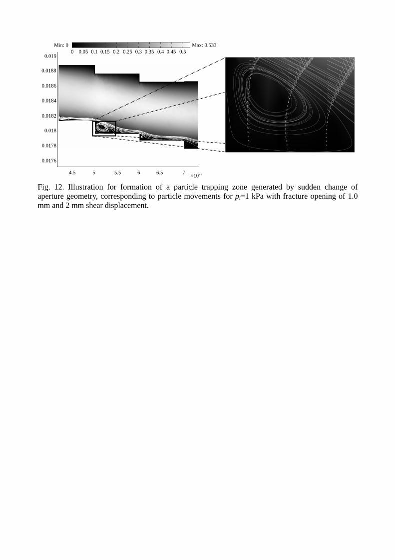
Fig. 12. Illustration for formation of a particle trapping zone generated by sudden change of aperture geometry, corresponding to particle movements for pi=1 kPa with fracture opening of 1.0 mm and 2 mm shear displacement.

4.5 5 5.5 6

0.018

0.0178

0.0184

0.0182

0.0188

0.0186

0.019

Min: 0 0.50 0.40.3 0.25 0.2

Max: 0.5330.450.35 0.15 0.1 0.05

0.0176

6.5 7 ×10-3

title reynolds equations for modeling the fluid flow and...

Documents