title: li and turner modified model for predicting liquid
TRANSCRIPT
Vol.:(0123456789)1 3
Journal of Petroleum Exploration and Production Technology (2019) 9:1971–1993 https://doi.org/10.1007/s13202-018-0585-6
ORIGINAL PAPER - PRODUCTION ENGINEERING
Title: Li and Turner Modified model for Predicting Liquid Loading in Gas Wells
Princewill Maduabuchi Ikpeka1 · Michael Onyinyechukwu Okolo1
Received: 22 August 2018 / Accepted: 2 November 2018 / Published online: 27 November 2018 © The Author(s) 2018
AbstractBackground Liquid loading of gas wells causes production difficulty and reduces ultimate recovery from these wells. Sev-eral authors proposed different models to predict the onset of liquid loading in gas wells, but the results from the models often show discrepancies. Turner’s et al. (J Pet Technol, 1969) critical model was developed based on the assumption that the droplet is a sphere and remains spherical all through the entire wellbore. On the other hand, Li’s model was developed based on the assumption the liquid droplets are flat in shape and remains same all through the wellbore. However, it is a well-known fact that the droplet alternates between spherical and flat during production operation. Invariably, the Turner’s model and the Li’s model would not be able to predict correctly the critical rate required to lift that droplet which is because the droplet deformation was not taken into account during the development of the models.Materials and methods In this work, a new improved model is developed and incorporated into Ms-Excel program to predict liquid loading in gas wells. In the new model, a deformation coefficient “C” is introduced to cater for the deformation of the liquid droplet along the wellbore and in turn be able to predict correctly the critical rate when the droplet varies from the spherical shape to the flat shape.Results Results from the analysis carried out revealed 35% error on from Turner’s model, 26% error on Li’s model, whereas the new model yielded 20% error.Conclusion The new developed software and model proved to be more accurate in predicting onset of liquid loading.
Keywords Predicting liquid loading in gas wells · Liquid loading · Gas production · Ms-Excel program · New improved model · Turner model · Li model · Gas wells · Production challenges in gas wells
List of symbols�l Liquid density, lbm/ft3
�g Gas density, lbm/ft3
� Interfacial tension, dynes/cmP Pressure, lbf/ft2
DH Hydraulic diameter, ftA Cross-sectional area of conduit, ft2
T Temperature, °Rz Gas compressibility factorSg Specific gravity of gasSO Specific gravity of produced oilSw Specific gravity of produced water
Ss Specific gravity of produced solidQg Gas production rate, Mscf/DQo Oil production rate, B/DQw Water production rate, B/DQs Solids production rate, ft3/dayphf Wellhead flowing pressure, psiaQgm Minimum gas flow rate required to transport
liquid drops, Mscf/DEkm Minimum kinetic energy required to transport
liquid drops, lbf-ft/ft3
Vcrit-S Critical velocity Luan’s modelVcrit-W Critical velocity Wang’s modelVcrit-L Critical velocity Li’s modelVcrit-N Critical velocity Nosseir’s modelVcrit-T Critical velocity Turner’s modelVcrit-C Critical velocity Coleman’s modelVcrit-new Critical velocity new modelWe Webers numberRe Reynolds number
* Princewill Maduabuchi Ikpeka [email protected]
Michael Onyinyechukwu Okolo [email protected]
1 Department of Petroleum Engineering, Federal University of Technology, Owerri, Nigeria
1972 Journal of Petroleum Exploration and Production Technology (2019) 9:1971–1993
1 3
ρ Density, lb/cu ftν Flow velocity, ft/s
Introduction
Background of study
Natural gas can be simply defined as a naturally occurring mixture of light hydrocarbons consisting mainly of methane but also contains varying amounts of heavier alkanes and other impurities such as carbon dioxide, hydrogen sulphide, helium, nitrogen and water. Natural gas exists in reservoir in different thermodynamic states; as dry gas, wet gas and as retrograde condensate. Although natural gas consumption in Nigeria is quite small compared to some countries such as the US, natural gas production is faced with variety of challenges one of which is the issue of liquid loading. Liquid loading, in a nutshell can be defined as the accumulation of liquid or water in the wellbore due to insufficient gas veloc-ity to evacuate the liquid phase which is co-produced with the gas resulting in reduction or complete cessation of gas production. These usually occur due to depletion of the res-ervoir pressure and at this stage the gas produced is unable to lift the liquid produced alongside it, to the surface and at such causing an accumulation of the liquid in the wellbore, and overtime as the liquid accumulates it builds up a high hydrostatic pressure in the wellbore thereby preventing fur-ther production of gas. Liquid loading leads to the premature death of a gas well which becomes a financial loss to the operating company.
The liquid content in the gas come from a variety of sources either in liquid form or in vapour form depending on the prevailing well conditions, some sources are; free water present in the formation produced alongside the gas, water condensate and hydrocarbon condensate which enter the well as vapour but while travelling up the tubing con-denses, in a case where the well completion is an open one, water or other liquid can flow from other zones into the well bore, in a case where there is an aquifer below the gas zone.
Liquid loading is not always easy to predict and recog-nize because a thorough diagnostic analysis of the well data needs to be done but accurate prediction of the problem is vitally important for taking timely measures to solve the problem. There are some symptoms also which can help predict a gas well which is under attack such as the onset of liquid slugs at the surface of the well, increasing difference between the tubing and casing pressures with time, sharp changes in gradient on a flowing pressure survey and sharp drops in production decline curve.
In a bid to predict the onset of liquid loading early which has been identified as the key step in salvaging the liquid loading problem, various investigators over the years have
come up with models and methods to predict liquid loading in gas wells, the pioneer been Turner et al. (1969) subse-quently other predictions came up most based on the founda-tion principle of Turner et al. (1969). Some of these models were better, some worse, but the various models used for the predictions had their merits and demerits. The Turner model and other models used in predicting liquid loading are included in subsequent sections.
After detection of liquid accumulation in the well, few solutions have been discovered to solve the problem of liq-uid loading in gas wells over the years and they have proved really helpful. These include foaming of the liquid water which can enable the gas to lift water from the well, the use of reduced tubing diameter and the heating the wellbore to the prevent further condensation, the use of plunger lift which is an intermittent artificial lift method which uses the energy of the gas reservoir to produce the liquid col-lected at the bottom of the hole, the use of gas lift method which involves injection of gas into the well from another source in other to increase gas production the use of the beam pumping which is a method commonly used in the oil industry to solve liquid loading in wells loaded with liquid hydrocarbon.
Statement of problem
From the above definition of liquid loading, it is clear that it is problematic to gas wells, ranging from decreasing the gas well production rate to completely preventing gas production from the well. However, if liquid loading can be predicted accurately and on time a suitable solution can be put together to combat it. This prediction in question is the primary aim of this study and research, due to the fact that the predicting methods at various points and times show various discrepan-cies, coming up or developing a better prediction mechanism will go a long way in saving maybe hundreds of petroleum gas wells which would have shut down prematurely due to liquid loading.
Aim of the study
This study aims at developing a new model for predicting critical velocity rate for gas wells building on the premise of Turner et al. (1969) and Li et al. (2001). The model devel-oped would then be incorporated into an Ms-Excel-based program.
Significance of study
As was earlier stated, that early detection of liquid load-ing in gas wells helps the production team prepare a suit-able technique and method to tackle the problem at its early stage before it aggravates. On the completion of this study,

1973Journal of Petroleum Exploration and Production Technology (2019) 9:1971–1993
1 3
software which when provided with the necessary data has the ability to predict liquid loading status of a given well will be developed.
Materials and methods
This research work was done on a three-phase scale:
1. Gathering of the various prediction model, evaluating their errors and choosing the better one.
2. Discover the merit and demerit of the chosen model and improve on it.
3. Finally build it into an excel platform for easy usage.
Predicting liquid loading
Liquid load-up in gas wells is not always obvious; there-fore, a thorough diagnostic analysis of well data needs to be carried out to adequately predict the rate at which liquids will accumulate in the well. Although this subject has been studied extensively but the results from previous investiga-tors and the most commonly applied model in the industry still has a high degree of inaccuracy, especially in predicting the minimum gas flow rate required to prevent liquid loading into the well bore (Adesina et al. 2013).
Turner’s model
For the removal of gas well liquids, Turner et al. (1969) pro-posed two physical models: (1) the continuous film model (2) and entrained drop movement model.
The continuous film model Turner et al. (1969) were of the opinion that since liquid film accumulation on the walls of a conduit during two-phase gas/liquid flow is inevitable due to the impingement of entrained liquid drops and the con-densation of vapours. He also suggested that the annular liq-uid film must keep moving upwards along the conduit walls to keep a gas well from loading up, and in the same vain the minimum gas flow rate necessary to accomplish this is of primary importance in the prediction of liquid loading. The analysis technique used involves describing the profile of the velocity of a liquid film moving upward on the inside of a tube. The major shortcoming of this model was its inabil-ity to clearly define between the adequate and inadequate rates when it was analysed with field data.
Entrained drop movement model (spherical shape droplet model) The existence of liquid drops in the gas stream pre-sents a different problem in fluid mechanics, namely, that of determining the minimum rate of gas flow that will lift the drops out of the well (Turner et al. 1969). In a bid to do this,
Turner et al. proposed a model to calculate the minimum gas flow velocity necessary to remove liquid drops from a gas well which is based on the sole principle of a freely falling particle in a fluid medium (by a transformation of coordinates, a drop of liquid being transported by a moving gas stream becomes a free falling particle and the same general equations apply as shown in Fig. 1). The minimum gas flow velocity necessary to remove liquid drop is given by the following equation:
Turner et al. (1969) discovered that the drop model pre-diction in most cases was too low and he blamed this on the values of critical weber number and drag coefficient used in the development of the model and also on the fact that the mathematical development predicts stagnation velocity, which must be exceeded by some finite quantity to guarantee removal of the largest droplets. Analysis of the Turner’s data reveals that the total contribution of these factors requires an upward adjustment of approximately 20%. Mapping Turn-er’s calculated model against actual test data (as shown in Fig. 2) reveals large discrepancies at lower flowrates; hence adjusted droplet model is given by the following equation to accommodate these discrepancies:
Coleman model
Coleman et al. (1991) made use of the Turner model but validated with field data of lower reservoir and wellhead
(1)Vcrit-Tunadjusted = 1.593�1∕4(�L − �g)
1∕4
�1∕2g
.
(2)Vcrit-T = 1.92�1∕4(�L − �g)
1∕4
�1∕2g
,
(3)qcrit-T =3060PVcrit-TA
Tz.
Fig. 1 Entrained droplet movement (Turner et al. 1969)

1974 Journal of Petroleum Exploration and Production Technology (2019) 9:1971–1993
1 3
flowing pressure all below approximately 500 psia. Cole-man et al. (1991) discovered that a better prediction could be achieved without a 20% upward adjustment to fit field data with the following expressions:
Li’s model (flat‑shaped droplet model)
Li et al. (2001) in their research posited that Turner and Coleman’s models did not consider deformation of the free falling liquid droplet in a gas medium, and furthermore, con-tended that as a liquid droplet is entrained in a high velocity gas stream, a pressure difference exists between the fore and aft portions of the droplet leading to its deformation and its shape changes from spherical to convex bean with unequal sides (flat) as shown in Fig. 3.
Spherical liquid droplets have a smaller efficient area and need a higher terminal velocity and critical rate to lift them to the surface. However, flat-shaped droplets have a more efficient area and are easier to be carried to the wellhead. This lead to the formulation of the following expression:
(4)Vcrit-C = 1.593
[�(�L − �g
)
�2g
] 1
4
,
(5)qcrit-C =3060PVcrit-CA
Tz.
(6)Vcrit-L =0.7241�1∕4(�l − �g)
1∕4
�1∕2g
,
(7)qcrit-L =3060PVcrit-LA
Tz.
Nosseir’s model
Nosseir et al. (2000) focused his study mainly on the impact of flow regime and changes in flow conditions on gas well loading. Their work was similar to that of Turner but the difference between the both was that Turner did not consider the effect of flow regime on the drag coefficient (used in the derivation stage), and thereby making use of the same drag coefficient (0.44) for laminar, transient and turbulent flows. Nosseir derived the critical flow equations by assuming drag coefficient value of 0.44 for Reynolds number (Re) 2 × 10⁵ to 104 and for Re value greater than 106 he took the drag coef-ficient value to be 0.2. Representation of the critical velocity equation by Nosseir’s model is summarized as:
Disk‑shaped droplet model
Some authors consider that the four dimensionless numbers, Reynolds, Mortan, Eotvos, and Weber (especially the first two parameters), are always used to characterize the shape of bubbles or droplets moving in a surrounding fluid or con-tinuous phase (Hinze 1955; Youngren and Acrivos 1976; Acharya et al. 1977). Wang and Liu (2007) were of the opin-ion that for typical oilfield condition, the Reynolds number
(8)Vcrit-N = 1.938
[�(�l − �g)
�2g
]1∕4
,
(9)qcrit-N =3060PVcrit-NA
Tz.
Fig. 2 Turner et al. model-calculated minimum flow rates mapped against the test flow rates (Guo et al. 2006)
Fig. 3 a Flat-shaped droplet model. b Shape of entrained droplet moving in high velocity gas (Li et al. 2001)

1975Journal of Petroleum Exploration and Production Technology (2019) 9:1971–1993
1 3
ranges from 104 to 106, and the Morton number for low viscosity liquid in gas wells is possibly between 10−10 and 10−12. For the given ranges of the dimensionless numbers, they found that most of the entrained droplets in gas well are disk shaped. Similar to flat-shaped droplets proposed by Li et al. (2001), the disk-shaped droplets have a more efficient area and are more easily carried to the wellhead. For the disk-shaped droplets, the drag coefficient Cd is close 1.17. Wang’s expressions can be summarized as follows:
Guohua and Shunli’s model
In this work, Guohua and Shunli (2012) carried out reviews on various models spotting their merit and shortcomings but paid much attention to the Turner’s model (spherical shaped droplet model) and Li’s model (flat shaped droplet model).
(10)Vcrit-W = 0.5213
[�(�l − �g)
�2g
]1∕4
,
(11)qcrit-W =3060PVcrit-WA
Tz.
Guo’s model
Guo et al. (2006) were of the opinion that although various investigators have suggested several methods of predicting liq-uid loading but the results from these methods often show dis-crepancies and are not easy to use due to the difficulties with prediction of the bottom hole pressure in multiphase flow.
Guo et al. (2006) formulated a closed form analytical equation for predicting the minimum gas flow rate for the continual removal of liquid from the gas well. He did this by substituting the Turner et al.’s entrained drop movement model (for predicting minimum gas velocity for the con-tinual removal of liquid from the gas well) into the kinetic energy equation to obtain the minimum kinetic energy the gas must possess in other to keep the well unloaded. The final stage of his work was to apply the minimum kinetic energy equation to the four phase mist flow model in gas wells to obtain the equation for predicting the minimum gas flow rate which can be solved using numerical method (Newton Raphson) or the go seek function built in the MS Excel. Below is a summary of Guo’s model:
(13)qcrit-S =3060PVcrit-SA
Tz,
(14)
b
�6.46 × 10⁻¹³
SgTQ2gm
A2Ekm
− phf
�+
1 − 2bm
2ln
����������
�6.46 × 10⁻¹³
SgTQ2gm
A2Ekm
+ m
�2+ n
�Phf + m
�2+ n
����������
−m +
b
cn − bm2
√n
⎡⎢⎢⎢⎣tan−1
⎡⎢⎢⎢⎣
6.46 × 10⁻¹³SgTQ
2gm
A2Ekm
+ m
√n
⎤⎥⎥⎥⎦− tan−1
�Phf+m√
n
�⎤⎥⎥⎥⎦= a
�1 + d2e
�L,
(14a)
a =15.33SSQS + 86.07SwQw + 86.07SOQO + 0.01879SgQg
TQg
cos(�),
(14b)
b = n =c2e
(1 + d2e)2
0.2456Qs + 1.379Qw + 1.379Qo
TQg
,
(14c)c =4.712 × 10⁻⁵TQg
A,
(14d)d =Qs + 5.615
(Qw + QO
)86400A
,
(14e)e =f
2gDH cos(�),
Using experimental results from Awolusi (2005) and Wei et al. (2007) (both though did different experiments came out with the same conclusion), Guohua and Shunli (2012) discovered that the Turner’s model overestimated the prob-ability of the occurrence of liquid loading in gas wells and Li’s model underestimated after a plot of critical gas flow rate was done against flow tubing pressure, for measured flow rates and calculated flow rates from Turner’s and Li’s model.
Guohua and Shunli (2012) came up with a dimensionless parameter of loss factor S which he introduced to his new model and using data from Coleman’s work. This loss factor S ranges from zero to unity (the larger it is, the closer the calculated results are to Turner’s model and if zero the new model matches Li’s model). Luan compared results from his work with Turner and Li and discovered that his was more accurate. Summary of Luan model given below:
(12)Vcrit-S = Vcrit-L + 0.83 × (Vcrit-T − Vcrit-L),
1976 Journal of Petroleum Exploration and Production Technology (2019) 9:1971–1993
1 3
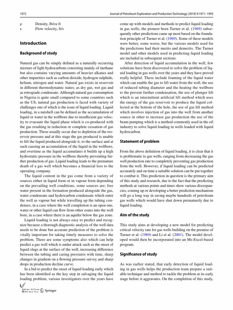
Nodal analysis
Nodal analysis can be used to estimate the onset of liquid loading in gas wells with more accuracy since it considers the complete flow path of fluids from reservoir to wellhead (Nallaparaju et al. 2012). In nodal analysis, the system is divided into two subsystems at a certain location called nodal point. The first subsystem takes into account inflow from reservoir to nodal point (IPR), while the other sub-system considers outflow from the nodal point to the sur-face (TPR). The curves formed by this relation on the pres-sure–rate graph are called the inflow curve and the outflow curve, respectively. The point where these two curves inter-sect denotes the optimum operating point where pressure and flow rate are equal for both of the curves. Turner’s criti-cal rate prediction in relation with the IPR and TPR curves can be used to predict liquid loading.
In a study carried out by Nallaparaju et al. 2012, we observe that Turner’s critical rate model was plotted with IPR and TPR for a Well with a given initial static reservoir pressure of 3281 psi and Tubing head pressure of 1500 psi as shown in Fig. 4 above. The point at which the Turner’s curve meets with the IPR curve represent the minimum flowrate to prevent liquid loading (10MMSCFD), whereas the optimum operating flowrate for the well is around 75MMSCFD. The
(14f)f =
⎡⎢⎢⎢⎣1
1.74 − 2 log�2�
DH
�⎤⎥⎥⎥⎦
2
,
(14g)m =cde
1 + d2e,
(14h)n =c2e
(1 + d2e)2.
farther the operating point from the minimum flowrate, the lower the tendency for liquid loading to occur.
Zhou model
Turner et al. (1969) entrained droplet model is the most pop-ular model in predicting liquid loading in gas wells (Zhou and Yuan 2009). However, there were still quite a few wells that could not be covered even after a 20% upward adjust-ment (Turner et al. 1969). By studying the droplet model and liquid film mechanisms, Zhou came up with a new model.
In his work, he studied the force balance on a single liquid droplet, which are the upward drag force, FD; the upward buoyant force, FB; and downward gravity force, FG, which
Fig. 4 IPR and TPR overlap with Turner (Nallaparaju et al. 2012)
Fig. 5 Encountering two liquid droplets in turbulent gas stream
Fig. 6 Liquid loading when liquid droplet number reaches a threshold value (Zhou and Yuan 2009)
1977Journal of Petroleum Exploration and Production Technology (2019) 9:1971–1993
1 3
for unloading to be possible and for the droplets to move upwards (FD + FB) must be greater than FG otherwise the droplet will accelerate downwards. The Turner et al. (1969) droplet model was based on the balance of these forces (FD+FB=FG).
Zhou argued that Turner et al. (1969) based his model on force balance on a single liquid droplet, but which in a gas stream, there are more than one as shown above (droplets A and B in Fig. 5). And further argued that if a turbulent flow existed in the gas stream, due to the irregularity of the flow droplets will encounter each other and coalesces will occur as in Fig. 6 below forming a droplet AB (A + B). This newly formed droplet in a situation the gas stream does not have enough energy to lift the droplet it starts falling and may scatter into smaller droplets 1, 2, 3 and the cycle goes on and on for similar larger droplets and these leads to an accumulation of liquid down hole.
Zhou and Yuan (2009) were of the opinion that if there are more liquid droplets in the gas stream, the chance of the process of liquid droplet encountering, coalescing, falling and scattering increases (Fig. 6). As the number of liquid droplets in a gas stream, called liquid droplet concentra-tion increases to a threshold value β, the process of drop-lets encountering, coalescing, falling and scattering will continue and bring those liquid droplets down to the well bottom. The liquid droplet concentration in a gas stream is defined by
Zhou and Yuan (2009) concluded that if liquid droplet concentration is above the threshold value, then the new model can be used but below the threshold value Turners model is used. Summary of Zhou model:
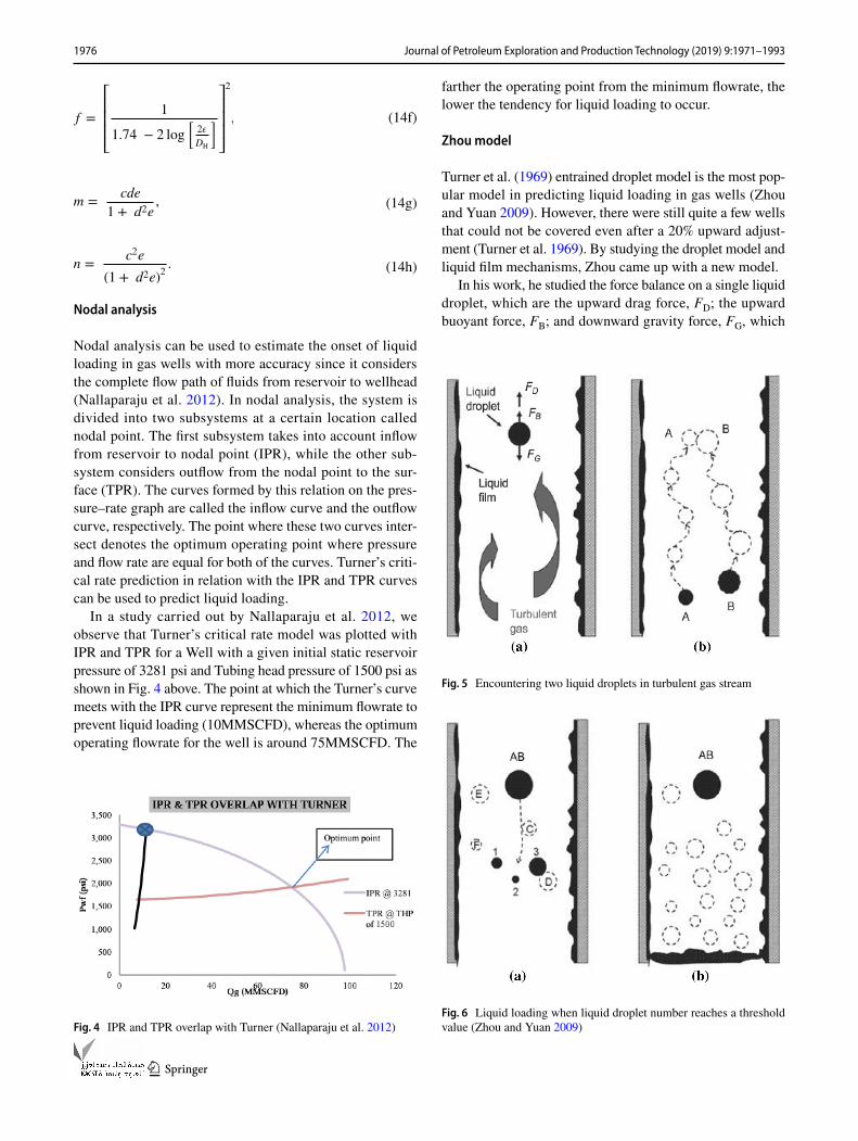
Experimental works on liquid loading
A series of experiments have been designed by Awolusi (2005) and Wei et al. (2007) which were done separately.
(15)
Hl =Liquid superficial velocity
Gas superficial velocity+liquid superficial velocity
=
Vsl
Vsg + Vsl
.
(16)Vcrit-Z = Vcrit-T = 1.593
[�(�l − �g)
]1∕4
�1∕2g
for Hl ⩽ �,
(17)Vcrit-Z = Vcrit-T + lnHl
𝛽+ 𝛼 for Hl > 𝛽,
(18)Q
(Mcf
D
)
crit-Z
=3060PVcrit-ZA
TZ.
The primary aim of their work was to investigate and evalu-ate discrepancies in the previous works on critical gas velocities required to keep liquid from accumulating. Which resulted to the discovery that Turner model prediction was high compared to the actual observed critical rate, while Li’s model prediction was low compared to the actual observed critical rate as can be seen in Fig. 7 below.
Model development
As was earlier stated at the beginning of this chapter, we are aimed at developing a new model which can be used to calculate the critical rate and in turn predict the onset of liquid loading in gas wells.
This new model was developed by combining the Turner critical rate model and the Li’s critical rate model.
Theory
(19)Vcrit-T = 1.593
[�(�l − �g
)
�2g
] 1
4
.
Fig. 7 Critical rate against flow tubing pressure (Awolusi 2005)
Fig. 8 Droplet shapes

1978 Journal of Petroleum Exploration and Production Technology (2019) 9:1971–1993
1 3
Turner’s critical model given above was developed based on the assumption that the droplet is a sphere and remains spherical all through the entire wellbore,
On the other hand, Li’s model above was developed based on the assumption that the liquid droplets are flat in shape and remains same all through the wellbore. Having considered the two above droplet shape, in a case where the droplet is neither spherical nor flat as can be observed in Fig. 8 invariably the Turner’s model and the Li’s model would not be able to pre-dict correctly the critical rate required to lift that droplet which is because the droplet deformation was not taken into account during the development of the models. As the droplet travel up the wellbore they tend to deform and can take different shapes at different points in the well. For simplicity sake, the only droplet shapes consider in this paper are droplet shapes ranging from the spherical shape to the flat shape (Fig. 9).
In the new model, a deformation coefficient C is intro-duced to cater for the deformation of the liquid droplet along the wellbore and in turn be able to predict correctly the criti-cal rate when the droplet varies from the spherical shape to the flat shape.
New model development
(20)Vcrit-L =0.7241�1∕4(�l − �g)
1∕4
�1∕2g
.
(21)
New critical velocity model
= Li�s critical velocity model + deformation
coefficient × (Turner’s critical velocity model
− Li’s critical velocity model),
The deformation coefficient used in this work is adapted from Kelbaliyev and Ceylan (2007). Detailed derivation of the deformation coefficient can be found in “Appendix 5”.
Using the experimental data from Raymond and Rosant (2000), �v is estimated as:
Weber’s number can be obtained from
(22)Vcrit-new = Vcrit-L + C × (Vcrit-T − Vcrit-L).
(23)C =a0
b0=
R(1 − �vWe
)
R(1 + �v
/2We
) .
(24)�v =1
12
(1 −
3 We
25 Re
).
(25)We =� × v2l
�,
Fig. 9 User interface for LOADCALC Software
Table 1 Summary of all assumptions used to prepare critical velocity rate for our new model
The condensate surface tension and density are used to calculate only when condensate is produced along with the gasThe water surface tension and density are used to calculate when only water is produced or when both water and condensate are produced along with the gas
Parameters Value Unit
Condensate surface tension 20 Dynes/cmWater surface tension 60 Dynes/cmCondensate density 45 Lb/cu ftWater density 67 Lb/cu ftGas specific gravity 0.6Wellhead temperature 580 Rankine

1979Journal of Petroleum Exploration and Production Technology (2019) 9:1971–1993
1 3
whereas Reynolds number is obtained from
Computing the values of Table 1 into Eqs. (35) and (36), the value of C was calculated to be:
C = 2.261921523
The derivation of the Turner and Li models is shown in “Appendix 1”.
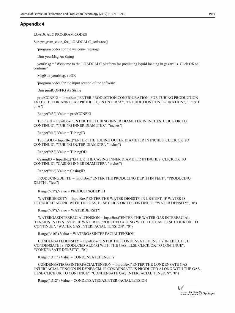
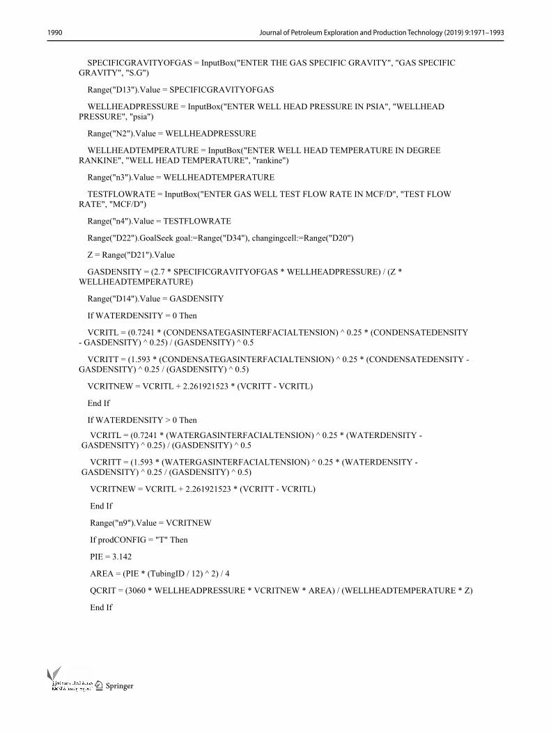
Software development
After the new model was developed, the new model and other related correlations were converted to computer codes and built into an excel platform leading to the development of a new software LOADCALC. The computer codes used for the development of LOADCALC are shown in appendix D.
LOADCALC features
LOADCALC software is colourful software and it is user friendly and consists of various sections;
a. Wellbore data sectionb. Fluid properties sectionc. Introductory sectiond. Flow parameter sectione. Output sectionf. Analysis section
Results
In other to be able to compute the critical rate using the new model and also compare with the critical rate from Turner and Li, the Turner et al. (1969) data on liquid loaded wells were utilised. Turner published important parameters which influence critical liquid loading rate calculation such as pro-ducing depth, wellhead pressures, liquid gas rate, fluid prop-erties, tubing inner/outer diameter, casing diameter and also
(26)Re =QDH
vA.
Vcrit-new = Vcrit-L + 2.261921523 × (Vcrit-T − Vcrit-L),
Vcrit-new =0.7241�1∕4(�l − �g)
1∕4
�1∕2g
+ 2.261921523
×
[1.593�1∕4(�l − �g)
1∕4
�1∕2g
−0.7241�1∕4(�l − �g)
1∕4
�1∕2g
],
(27)qcrit-new =3060PVcrit-newA
Tz= Critical flow rate.
0
2000
4000
6000
8000
10000
12000
14000
0 2000 4000 6000 8000 10000 12000 14000
Test
flow
rate
(mcf
/d)
Cri�cal flow rate(mcf/d)
Li's model
loaded up
Near L.U
Unloaded
Fig. 10 Crossplot of test flowrate against critical flowrate using Li’s model
0
2000
4000
6000
8000
10000
12000
14000
0 2000 4000 6000 8000 10000 12000 14000
Test
flow
rate
(mcf
/d)
Cri�cal flow rate(mcf/d)
Turner's model
Loaded up
Near L.U
Unloaded
Fig. 11 Crossplot of test flowrate against critical flowrate using Turner model
information on the well flow rate and status (loaded up, near load up and unloaded) at time of test was also included in the database. These data are shown in “Appendix 3”.
Assumptions
All assumptions are summarized in Table 1 below;
Calculated parameters
Due to the large amount of database, the calculations for the below parameters are done using an excel sheet.
Parameters
a. Gas densityb. Production areac. Compressibility factor
The results for the calculated parameters, formulas, cor-relations used in calculation are all stated and outlined in “Appendix 2”.

1980 Journal of Petroleum Exploration and Production Technology (2019) 9:1971–1993
1 3
Critical velocity results
Using the production data from the 105 gas wells, assumed parameters and calculated parameter, an excel sheet was used to compute the critical rate for.
• The new critical velocity model.• The Turner critical velocity model.• The Li’s critical velocity model.
The results from the different critical velocity models are tabulated in “Appendix 2”.
When the measured flow rate from the different gas wells was plotted against the critical flow rates from the differ-ent models in the above table, the following figures were obtained, Figs. 10, 11, 12.
Discussion
The above figures are constructed in such a way that if a well’s actual test flow rate equals its critical flow rate for liquid removal, the point will plot on the diagonal, so there-fore for critical velocity model to be correct, the wells that are tested at conditions near load-up should plot near this diagonal. Wells that unload easily during a test should plot above the diagonal and those that do not unload should plot below the line. The ability of a given analytical model to achieve this data separation is a measure of its validity.
As can be seen from Figs. 10, 11 and 12 above the most data separation is achieved by the new model in Fig. 12 and in turn provides a better prediction.
Li’s model as can be seen in Fig. 10 was not able to sepa-rate the loaded wells from the unloaded wells, almost all the points plotted above the diagonal line, suggesting that all the wells are unloaded which is not correct compared to the well status obtained from the different wells during test.
Turner model as can be seen in Fig. 11 predicted better than Li but majority of the loaded wells still plotted in the unloaded region above the diagonal line.
From Fig. 12, it can be observed that the new model pre-diction was quite better than Turner and Li due to the fact that most of the loaded wells plotted in the loaded region, most of the unloaded wells plotted in the unloaded region and the near load up wells plotted close to the diagonal.
Software test
To test the efficiency of the LOADCALC software, the well data from a loaded well, an unloaded well and a well which is near load up was collected and feed in the software.
The summary of the production data from the three dif-ferent wells is shown in Table 2.
0
2000
4000
6000
8000
10000
12000
14000
0 2000 4000 6000 8000 10000 12000 14000
Test
flow
rate
(mcf
/d)
Cri�cal flow rate(mcf/d)
New model
loaded up
Near L.U
Unloaded
Fig. 12 Crossplot of test flowrate against critical flowrate using New model
Table 2 Summary of the production data from the three different wells
Well status Loaded up Near load up Unloaded
Producing depth (ft) 2250 6770 6180Wellhead pressure (psia) 210 450 1117Wellhead temperature (rankine) 580 580 580Tubing ID (in.) 0 1.995 0Tubing OD (in.) 2.375 0 2.878Casing ID (in.) 6.276 0 6.184Production configuration Annular Tubular AnnularSpecific gravity 0.6 0.6 0.6Water density (lb/cu ft) 67 0 0Water surface tension (dynes/cm) 60 0 0Condensate density (lb/cu ft) 0 45 45Condensate surface tension (dynes/cm) 0 20 20Test flow rate (mcf/days) 470 442 5513Critical flow rate(mcf/days) 2593.59 685.20 2928.38

1981Journal of Petroleum Exploration and Production Technology (2019) 9:1971–1993
1 3
Fig. 13 LOADCALC software interface showing loaded up test
Fig. 14 LOADCALC software interface showing near load up test

1982 Journal of Petroleum Exploration and Production Technology (2019) 9:1971–1993
1 3
Loaded up test
See Fig. 13.
4.3 Near load up test
See Fig. 14.
Unloaded test
See Fig. 15.As can be observed from the test figures above the results
from the software matches with the test result in Table 2.
Conclusion
This paper presents a new empirical model that calculates the critical velocity and flowrate for low-pressure gas wells by taking into account droplet deformation coefficient. The new model is derived from a modification of Turner’s model and Li’s model. The Turner’s critical model above was devel-oped based on the assumption that the droplet is a sphere and remains spherical all through the entire wellbore On the other hand, Li’s model above was developed based on the assump-tion the liquid droplets are flat in shape and remains same all through the wellbore. By applying the deformation and elasticity theory, a dimensionless coefficient, C was obtained as a function of the gas Weber number and Reynolds number assuming the surface area of a particle increases after defor-mation, while the volume remains constant.
Comparative analysis of well test results obtained from 105 gas wells between the new model, Turner’s spherical
model and Li’s flat model reveal that droplet deformation plays an important role in the accuracy of prediction of criti-cal flowrate for liquid loading. Error analysis carried out reveals that the new model predicted the onset of liquid load-ing in gas wells with the least error of 20%, whereas Turner’s model had 26% error and Li, 35% error.
Finally, the recommended applicable range of the new model is when the wellhead pressure is less than 500 psia and the liquid/gas ratios are in the range of 1–130 bbl/MMscf, which is suggested by Turner et al. (1969) to ensure a mist flow in gas wells.
Open Access This article is distributed under the terms of the Crea-tive Commons Attribution 4.0 International License (http://creat iveco mmons .org/licen ses/by/4.0/), which permits unrestricted use, distribu-tion, and reproduction in any medium, provided you give appropriate credit to the original author(s) and the source, provide a link to the Creative Commons license, and indicate if changes were made.
Appendix 1
Development of the critical velocity models
Turner model
Since the liquid droplets are particles moving relative to a fluid in the gravitational field, particle mechanics may be employed to determine this minimum gas flow rate. A freely falling particle in a fluid medium will reach a terminal veloc-ity, which is the maximum velocity it can attain under the influence of gravity alone, i.e. when the drag forces equal the accelerating forces. Terminal velocity is therefore a func-tion of the size, shape and density of the particle and of the density and viscosity of the fluid medium.
Fig. 15 LOADCALC software interface showing unloaded test

1983Journal of Petroleum Exploration and Production Technology (2019) 9:1971–1993
1 3
By transformation of coordinates, a drop of liquid being transported by moving gas stream becomes a free falling particle and the same general equations apply.
Turner determined that it is the antagonism of two pres-sures, the velocity pressure and the surface tension pres-sure that determines the maximum size a drop may attain. The ratio of these two pressures is the weber number. Hinze showed that if the weber number exceeded a critical value, a liquid drop would shatter. Weber number was found to be on the order of 20–30. If the larger of observed values is used, a relationship between the maximum drop diameter and the velocity of a liquid drop is obtained.
Substituting the maximum diameter expression into Eq. 28, the terminal velocity equation becomes
The drag coefficient is inflected by the drop shape and the drop Reynolds number, for spheres laboratory results shows that for a Reynolds number ranges of 1000 to 200,000 the drag coefficient is approximately constant and the drag coef-ficient of 0.44 was used resulting to
Converting the surface tension from 1 lbf/ft to 0.00006852 dyne/cm equation becomes
(28)Vt = 6.55
√d(�l − �g)
�gCd
.
(29)dm =30�gc
�gV2t
.
(30)Vt =1.3�1∕4(�l − �g)
1∕4
C1∕4
d�1∕2g
.
(31)Vt =17.6�1∕4(�l − �g)
1∕4
�1∕2g
.
(32)Vt =1.593�1∕4(�l − �g)
1∕4
�1∕2g
.
Li’s model
Li argued that a pressure difference exists between the fore and aft portion of a free falling droplet. The droplet is thus deformed, under the applied forces, from a sphere to a con-vex beam shown in Fig. 16 above.
Equating the gravity of a liquid droplet to the buoyancy and drag force, we obtain (in SI units)
As the droplets fall relative to the gas stream velocity, the pressure difference existing between the fore and aft por-tions, by Bernoulli, is expressed as
The condition for the balance of pressure and interfacial tension force is
For a constant volume of the droplet, the following condi-tion must be satisfied:
From equation A8, we obtain
From Eq. 36, we have
By combining Eqs. 38 and 37, we calculate the thickness of the droplet as
Substituting Δp from Eqs. 34 into 39, we have
Hence, s is estimated to be
Substituting Eqs. 41 into 33 and solving for v = vc,
(33)�lgV = �ggV + 1∕2�gv2sCd.
(34)Δp =10−3�gv
2
2.
(35)(
Δp
10−3
)sΔh + �Δs = 0.
(36)V = sh = constant
(37)Δps
10−3�=
Δs
Δh.
(38)Δs
Δh= −
V
h2= −
sh
h2= −
s
h
(39)h =10−3�
Δp
(40)h =2�
�gv2.
(41)s =�gv
2V
2�.
(42)vc = v =4
√√√√4(�l − �g
)g�
�2gCd
.
Fig. 16 Buoyancy, drag and gravity forces acting on a liquid droplet (Li et al. 2001)

1984 Journal of Petroleum Exploration and Production Technology (2019) 9:1971–1993
1 3
For a typical field condition, the particle’s Reynolds num-ber ranges from 104.
To 105 and the drag coefficient (Cd) is close to 1.0 for the shape considered. Hence, we have
(43)vc = 2.5�1∕4(�l − �g)
1∕4
�1∕2g
.
When converted to field units, we have
Appendix 2
(44)vc = 0.7241�1∕4(�l − �g)
1∕4
�1∕2g
.
LI’s calculated Turner’s calculated New model
Critical velocity (ft/s)
Critical flow rate (mcf/days)
Critical velocity (ft/s)
Critical flow rate (mcf/days)
Critical velocity (ft/s)
Critical flow rate (mcf/days)
7.421352494 699.4091215 16.32677051 1538.680749 27.56470916 2597.775686.396371673 359.6368142 14.07184101 791.1910578 23.75768096 1335.7786464.131293989 2118.908919 9.088732668 4661.541097 15.34463124 7870.1433663.541108845 2462.936944 7.790341651 5418.39325 13.15253999 9147.9471733.386080896 2572.339805 7.449284445 5659.076522 12.57672846 9554.296023.291364351 2644.010978 7.240910662 5816.751123 12.22492816 9820.5001993.234436286 332.9551895 7.115670493 732.4922205 12.01348348 1236.6765994.715188246 202.0876575 10.3732839 444.5872647 17.5133566 750.60273844.059829716 1265.103589 8.93151324 2783.192953 15.07919553 4698.9025953.919333361 512.5407015 8.62242514 1127.575387 14.55735788 1903.7008933.758126787 533.7705151 8.267775131 1174.28039 13.95859744 1982.5535873.598854403 556.5083356 7.917380284 1224.302967 13.36702104 2067.0073863.053296867 651.0725861 6.717168773 1432.341706 11.34068759 2418.2420252.001478177 849.0393442 4.403196708 1867.863106 7.433977014 3153.538741.943962951 871.8746529 4.276664799 1918.100155 7.220351467 3238.3546331.684472966 1417.688544 3.705793999 3118.87564 6.256542516 5265.6402511.491075008 1100.566301 3.280323834 2421.215463 5.538215437 4087.7710651.456080213 1122.729251 3.203336252 2469.973342 5.408236253 4170.0896581.455257267 290.9181632 3.201525792 640.0119237 5.405179628 1080.5408541.400981857 300.2324567 3.082121389 660.5031122 5.203587548 1115.1364061.365227426 778.9730088 3.00346263 1713.719104 5.070786893 2893.295321.342980359 789.411588 2.954519697 1736.68369 4.988155872 2932.0667431.21719954 799.768578 2.677805368 1759.468782 4.520975299 2970.5351241.14102966 740.5246871 2.510233736 1629.133858 4.238061829 2750.4888961.120325183 750.4774926 2.464684459 1651.029755 4.161160365 2787.4560381.120009862 1127.752536 2.463990762 2481.024431 4.159989186 4188.7473611.092491886 510.4162589 2.403451973 1122.901672 4.057780724 1895.8101971.090396025 765.1843916 2.398841138 1683.384527 4.049996188 2842.081041.081265155 514.1588825 2.378753475 1131.13534 4.016081913 1909.7112111.073654413 773.5731771 2.362010054 1701.839623 3.987813767 2873.239030.821584786 910.0832924 1.807463838 2002.158106 3.051565831 3380.27081910.42094012 136.6487472 22.92578042 300.6234695 38.70590755 507.54670085.307834134 254.6612526 11.67708849 560.2477219 19.71458765 945.87386463.422057394 185.7565004 7.528431748 408.6591702 12.71035393 689.94484684.524866689 297.7395319 9.954581738 655.0187465 16.80645602 1105.8770774.47176837 450.9070705 9.837766901 991.9831008 16.60923594 1674.7785892.641855551 356.5982659 5.812009242 784.5063356 9.812494416 1324.4927391.709903977 1399.141035 3.76174152 3078.071631 6.350999478 5196.750286

1985Journal of Petroleum Exploration and Production Technology (2019) 9:1971–1993
1 3
LI’s calculated Turner’s calculated New model
Critical velocity (ft/s)
Critical flow rate (mcf/days)
Critical velocity (ft/s)
Critical flow rate (mcf/days)
Critical velocity (ft/s)
Critical flow rate (mcf/days)
1.556999679 274.7512183 3.425356288 604.4450915 5.783075706 1020.4928861.499996768 1095.037664 3.299951458 2409.052616 5.571353022 4067.2363651.475833132 1110.124946 3.246792128 2442.244219 5.481603401 4123.2742021.403547149 299.7808064 3.087764962 659.509494 5.213115669 1113.4588671.369620827 776.9387388 3.013127989 1709.243766 5.087105051 2885.7395461.348429142 434.714034 2.966506868 956.3588679 5.008393976 1614.6337111.34746222 787.2900433 2.964379665 1732.01635 5.004802591 2924.1868091.135442959 743.1923023 2.497943148 1635.002538 4.217311462 2760.3970681.129647046 1120.7564 2.485192299 2465.633124 4.19578403 4162.7620091.127202887 1122.525143 2.479815217 2469.524309 4.186705829 4169.3315491.121590491 749.8640298 2.467468101 1649.680154 4.165860025 2785.1774881.08818154 511.8490824 2.393969333 1126.053844 4.041771052 1901.1320521.076379387 772.1999559 2.36800492 1698.818574 3.997934981 2868.1385531.060167742 521.2849112 2.332339749 1146.812407 3.937720986 1936.1790160.828289561 906.3740504 1.822214156 1993.997876 3.076468996 3366.4937912.069910537 823.3000487 4.553746009 1811.237367 7.688151451 3057.9367331.943055426 317.051904 4.274668269 697.5054317 7.216980699 1177.6079271.756986123 347.0319721 3.865320942 763.4607535 6.525874028 1288.9611952.550365894 396.0331763 5.610734525 871.2620492 9.472679569 1470.9635921.729666199 1385.031745 3.805217863 3047.031583 6.424401181 5144.344952.488292397 405.1319773 5.474174545 891.2791601 9.242123494 1504.7587531.678272973 257.464428 3.692154187 566.4146304 6.233514235 956.28554031.630809828 370.5014663 3.587736578 815.0929925 6.057224563 1376.1326081.599159534 376.8453131 3.518106805 829.0492801 5.939667668 1399.6951991.584225405 379.9067787 3.485252133 835.7844198 5.884198678 1411.0662271.574311494 381.9637827 3.463441805 840.3097719 5.847376003 1418.7064412.279657719 570.3090674 5.015184016 1254.664196 8.467203527 2118.2666622.276833029 439.3267218 5.008969777 966.5066536 8.456711942 1631.7663561.535862442 390.1324084 3.378854952 858.2805229 5.704566866 1449.0467051.519721278 393.6544503 3.343344836 866.0289177 5.644614654 1462.1284251.516458703 394.3731698 3.336167261 867.6100809 5.632496656 1464.7979241.511372749 1088.058447 3.324978303 2393.69853 5.613606187 4041.3138521.493290761 1099.188691 3.285198429 2418.18476 5.546445282 4082.6542891.471562939 732.1496788 3.237397821 1610.709071 5.465742864 2719.3820772.110573533 470.2398351 4.643203477 1034.514649 7.839183713 1746.5851821.413206941 418.3594754 3.109016236 920.3792905 5.248994485 1553.88891.405757846 299.3925111 3.092628433 658.6552551 5.221326734 1112.0166441.392656745 325.8187734 3.063806374 716.7923022 5.172666058 1210.1702131.38625049 769.3187759 3.049712788 1692.480058 5.148871666 2857.4371492.046960152 483.1548332 4.503255796 1062.927288 7.602908137 1794.5546271.385191945 425.3032698 3.04738402 935.6554464 5.144939975 1579.6798421.374747968 774.5759431 3.024407558 1704.045681 5.106148501 2876.9635481.32615174 339.0168546 2.9174972 745.8277163 4.925650286 1259.1910991.323415957 441.3164356 2.911478551 970.8839689 4.915488919 1639.1566371.955275567 653.633251 4.301552242 1437.975099 7.262369277 2427.7529571.290926191 450.1400415 2.840001964 990.2956583 4.794814024 1671.9296571.282960346 452.3468883 2.822477325 995.1506602 4.765226936 1680.1264231.893367226 517.1644348 4.165355602 1137.747472 7.032426634 1920.8745641.890328167 517.8808064 4.158669756 1139.32347 7.021138828 1923.535343

1986 Journal of Petroleum Exploration and Production Technology (2019) 9:1971–1993
1 3
LI’s calculated Turner’s calculated New model
Critical velocity (ft/s)
Critical flow rate (mcf/days)
Critical velocity (ft/s)
Critical flow rate (mcf/days)
Critical velocity (ft/s)
Critical flow rate (mcf/days)
1.268325947 456.4463974 2.790282052 1004.169467 4.710871218 1695.3529971.257046614 353.6829155 2.765467832 778.0926451 4.668977031 1313.6644181.845859692 686.9283921 4.060840339 1511.223489 6.85597209 2551.4192141.226248479 360.5449216 2.697712783 793.1888691 4.554585259 1339.1515781.80973596 537.5436438 3.981369126 1182.581169 6.721799758 1996.5679061.208624311 804.1004949 2.658940101 1768.998879 4.489124812 2986.6249181.787904127 705.8110894 3.933339696 1552.764902 6.640711016 2621.5541471.175099571 724.545081 2.585186599 1593.979166 4.36460577 2691.136751.162399661 730.4436077 2.557247147 1606.955762 4.317435212 2713.0453141.105630712 506.0805299 2.432357028 1113.363188 4.106581521 1879.7062441.10253258 507.0985587 2.425541224 1115.602823 4.095074307 1883.4874511.100054031 507.9149264 2.420088484 1117.398809 4.085868371 1886.5196391.080199508 770.279937 2.376409082 1694.594586 4.012123842 2861.0071351.074300103 516.4981552 2.363430555 1136.281675 3.990212017 1918.3998391.474301242 825.382891 3.243422012 1815.819563 5.475913587 3065.6729161.451895651 835.1698762 3.19413033 1837.35066 5.39269377 3102.0241611.437724503 841.4514938 3.162954197 1851.170045 5.340058679 3125.3556171.426234667 846.5968816 3.137676874 1862.489756 5.297382631 3144.466840.843677721 897.8268281 1.856067683 1975.194223 3.133624365 3334.747328
Appendix 3
Turner’s data
Producing depth (ft)
Wellhead pressure (psi)
Condensate gravity (API)
Conden-sate make (bbl/MM)
Water make (bbl/MM)
Tubing ID (in.)
Tubing OD (in.)
Casing ID (in.)
Test flow rate (Mcf/D)
Well status dur-ing test
6529 108 64.3 9.6 12.4 2.041 568 Near L.U2250 210 0 0 24 2.375 6.276 470 Loaded up3077 280 0 0 28 2.375 4.974 500 Loaded up3278 315 50 10 0 7.386 5740 Loaded up6739 400 0 18 1.995 417 Near L.U3278 422 50 10 0 7.386 3890 Loaded up6770 450 61 11.3 0 1.995 442 Near L.U3278 459 50 10 0 7.386 2780 Loaded up3278 484 50 10 0 7.386 1638 Loaded up5080 500 50 14 0 2.375 4.974 400 Loaded up7200 500 0 0 5 2.375 4.052 800 Loaded up6700 540 70.8 10.5 10.5 1.995 712 Near L.U7531 552 54.9 25.1 22.3 2.441 1607 Near L.U6776 660 0 0 3.5 2.375 6.276 4300 Loaded up7531 704 54.9 31.6 40.8 2.441 1313 Loaded up6404 725 63.8 6 0 2.441 775 Near L.U7531 760 54.9 46.1 45.1 2.441 1247 Loaded up7531 822 54.9 26.7 26.3 2.441 1356 Loaded up7531 1102 54.9 26.1 23.8 2.441 1365 Loaded up
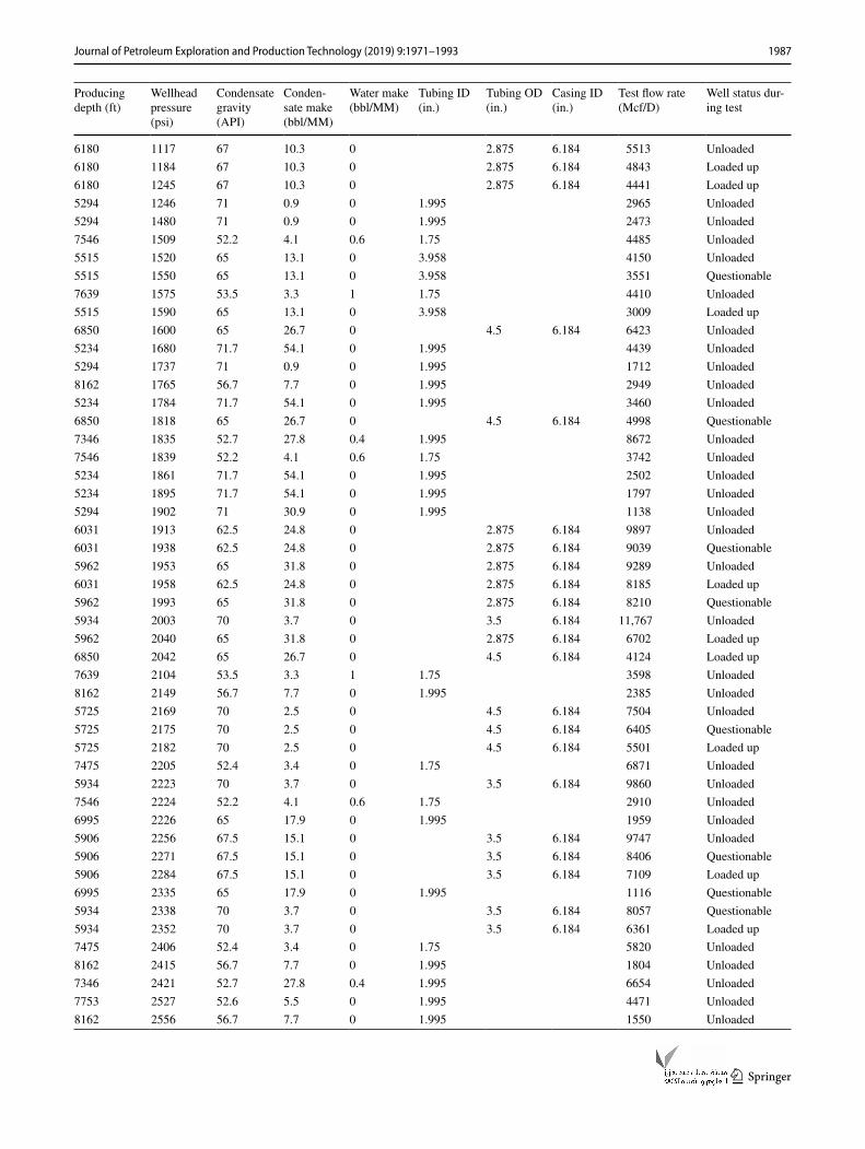
1987Journal of Petroleum Exploration and Production Technology (2019) 9:1971–1993
1 3
Producing depth (ft)
Wellhead pressure (psi)
Condensate gravity (API)
Conden-sate make (bbl/MM)
Water make (bbl/MM)
Tubing ID (in.)
Tubing OD (in.)
Casing ID (in.)
Test flow rate (Mcf/D)
Well status dur-ing test
6180 1117 67 10.3 0 2.875 6.184 5513 Unloaded6180 1184 67 10.3 0 2.875 6.184 4843 Loaded up6180 1245 67 10.3 0 2.875 6.184 4441 Loaded up5294 1246 71 0.9 0 1.995 2965 Unloaded5294 1480 71 0.9 0 1.995 2473 Unloaded7546 1509 52.2 4.1 0.6 1.75 4485 Unloaded5515 1520 65 13.1 0 3.958 4150 Unloaded5515 1550 65 13.1 0 3.958 3551 Questionable7639 1575 53.5 3.3 1 1.75 4410 Unloaded5515 1590 65 13.1 0 3.958 3009 Loaded up6850 1600 65 26.7 0 4.5 6.184 6423 Unloaded5234 1680 71.7 54.1 0 1.995 4439 Unloaded5294 1737 71 0.9 0 1.995 1712 Unloaded8162 1765 56.7 7.7 0 1.995 2949 Unloaded5234 1784 71.7 54.1 0 1.995 3460 Unloaded6850 1818 65 26.7 0 4.5 6.184 4998 Questionable7346 1835 52.7 27.8 0.4 1.995 8672 Unloaded7546 1839 52.2 4.1 0.6 1.75 3742 Unloaded5234 1861 71.7 54.1 0 1.995 2502 Unloaded5234 1895 71.7 54.1 0 1.995 1797 Unloaded5294 1902 71 30.9 0 1.995 1138 Unloaded6031 1913 62.5 24.8 0 2.875 6.184 9897 Unloaded6031 1938 62.5 24.8 0 2.875 6.184 9039 Questionable5962 1953 65 31.8 0 2.875 6.184 9289 Unloaded6031 1958 62.5 24.8 0 2.875 6.184 8185 Loaded up5962 1993 65 31.8 0 2.875 6.184 8210 Questionable5934 2003 70 3.7 0 3.5 6.184 11,767 Unloaded5962 2040 65 31.8 0 2.875 6.184 6702 Loaded up6850 2042 65 26.7 0 4.5 6.184 4124 Loaded up7639 2104 53.5 3.3 1 1.75 3598 Unloaded8162 2149 56.7 7.7 0 1.995 2385 Unloaded5725 2169 70 2.5 0 4.5 6.184 7504 Unloaded5725 2175 70 2.5 0 4.5 6.184 6405 Questionable5725 2182 70 2.5 0 4.5 6.184 5501 Loaded up7475 2205 52.4 3.4 0 1.75 6871 Unloaded5934 2223 70 3.7 0 3.5 6.184 9860 Unloaded7546 2224 52.2 4.1 0.6 1.75 2910 Unloaded6995 2226 65 17.9 0 1.995 1959 Unloaded5906 2256 67.5 15.1 0 3.5 6.184 9747 Unloaded5906 2271 67.5 15.1 0 3.5 6.184 8406 Questionable5906 2284 67.5 15.1 0 3.5 6.184 7109 Loaded up6995 2335 65 17.9 0 1.995 1116 Questionable5934 2338 70 3.7 0 3.5 6.184 8057 Questionable5934 2352 70 3.7 0 3.5 6.184 6361 Loaded up7475 2406 52.4 3.4 0 1.75 5820 Unloaded8162 2415 56.7 7.7 0 1.995 1804 Unloaded7346 2421 52.7 27.8 0.4 1.995 6654 Unloaded7753 2527 52.6 5.5 0 1.995 4471 Unloaded8162 2556 56.7 7.7 0 1.995 1550 Unloaded

1988 Journal of Petroleum Exploration and Production Technology (2019) 9:1971–1993
1 3
Producing depth (ft)
Wellhead pressure (psi)
Condensate gravity (API)
Conden-sate make (bbl/MM)
Water make (bbl/MM)
Tubing ID (in.)
Tubing OD (in.)
Casing ID (in.)
Test flow rate (Mcf/D)
Well status dur-ing test
7546 2574 52.2 4.1 0.6 1.75 1943 Unloaded7639 2582 53.5 3.3 1 1.75 2423 Unloaded7753 2611 52.6 5.5 0 1.995 3436 Unloaded7475 2655 52.4 3.4 0 1.75 4140 Unloaded7346 2705 52.7 27.8 0.4 1.995 5136 Unloaded7475 2783 52.4 3.4 0 1.75 2939 Unloaded7639 2814 53.5 3.3 1 1.75 1596 Unloaded7810 2823 52.2 5 0 2.375 4.974 3863 Loaded up7810 2862 52.2 5 0 2.375 4.974 3024 Unloaded7346 2884 52.7 27.8 0.4 1.995 3917 Unloaded8840 3025 60 54.8 0 2.441 3517 Unloaded11,355 3092 55 117.6 0 2.441 3351 Unloaded8840 3212 60 54.8 0 2.441 2547 Loaded up11,355 3245 55 117.6 0 2.441 2503 Questionable11,416 3280 56.4 130.8 0 2.992 4095 Questionable11,416 3295 56.4 130.8 0 2.992 3264 Questionable11,417 3330 56.4 113.5 0 2.441 2915 Questionable11,355 3338 55 117.6 0 2.441 2261 Loaded up11,416 3340 56.4 130.8 0 2.992 2611 Loaded up11,200 3434 61 37.4 0 1.995 2926 Unloaded11,390 3455 55 104.3 0 1.995 2769 Unloaded11,426 3472 55 106.9 0 1.995 2572 Unloaded11,426 3525 55 106.9 0 1.995 1792 Loaded up11,417 3540 56.4 113.5 0 2.441 1814 Loaded up11,390 3556 55 104.3 0 1.995 2069 Questionable11,200 3607 61 37.4 0 1.995 1525 Loaded up8690 3615 60 68.3 0 2.441 3890 Unloaded8690 3644 60 68.3 0 2.441 3182 Questionable11,340 3660 58 36.8 0 1.995 3726 Unloaded8690 3665 60 68.3 0 2.441 2542 Loaded up11,340 3773 58 36.8 0 1.995 2494 Questionable8963 4575 43.9 7.5 1.4 1.995 7792 Unloaded8963 4786 43.9 7.5 1.4 1.995 6221 Unloaded8963 4931 43.9 7.5 1.4 1.995 4830 Unloaded8963 5056 43.9 7.5 1.4 1.995 3376 Unloaded11,850 7405 67.5 10.8 0 2.441 6946 Unloaded11,850 7950 67.5 10.8 0 2.441 4896 Questionable11,850 8215 67.5 10.8 0 2.441 3472 Loaded up
1989Journal of Petroleum Exploration and Production Technology (2019) 9:1971–1993
1 3
Appendix 4
LOADCALC PROGRAM CODES
Sub program_code_for_LOADCALC_software()
'program codes for the welcome message
Dim yourMsg As String
yourMsg = "Welcome to the LOADCALC platform for predicting liquid loading in gas wells. Click OK to continue"
MsgBox yourMsg, vbOK
'program codes for the input section of the software
Dim prodCONFIG As String
prodCONFIG = InputBox("ENTER PRODUCTION CONFIGURATION, FOR TUBING PRODUCTION ENTER 'T', FOR ANNULAR PRODUCTION ENTER 'A'", "PRODUCTION CONFIGURATION", "Enter T or A")
Range("d3").Value = prodCONFIG
TubingID = InputBox("ENTER THE TUBING INNER DIAMETER IN INCHES. CLICK OK TO CONTINUE", "TUBING INNER DIAMETER", "inches")
Range("d4").Value = TubingID
TubingOD = InputBox("ENTER THE TUBING OUTER DIAMETER IN INCHES. CLICK OK TO CONTINUE", "TUBING OUTER DIAMETR", "inches")
Range("d5").Value = TubingOD
CasingID = InputBox("ENTER THE CASING INNER DIAMETER IN INCHES. CLICK OK TO CONTINUE", "CASING INNER DIAMETER", "inches")
Range("d6").Value = CasingID
PRODUCINGDEPTH = InputBox("ENTER THE PRODUCING DEPTH IN FEET", "PRODUCING DEPTH", "feet")
Range("d7").Value = PRODUCINGDEPTH
WATERDENSITY = InputBox("ENTER THE WATER DENSITY IN LB/CUFT, IF WATER IS PRODUCED ALONG WITH THE GAS, ELSE CLICK OK TO CONTINUE", "WATER DENSITY", "0")
Range("d9").Value = WATERDENSITY
WATERGASINTERFACIALTENSION = InputBox("ENTER THE WATER GAS INTERFACIAL TENSION IN DYNES/CM, IF WATER IS PRODUCED ALONG WITH THE GAS, ELSE CLICK OK TO CONTINUE", "WATER GAS INTERFACIAL TENSION", "0")
Range("d10").Value = WATERGASINTERFACIALTENSION
CONDENSATEDENSITY = InputBox("ENTER THE CONDENSATE DENSITY IN LB/CUFT, IF CONDENSATE IS PRODUCED ALONG WITH THE GAS, ELSE CLICK OK TO CONTINUE", "CONDENSATE DENSITY", "0")
Range("D11").Value = CONDENSATEDENSITY
CONDENSATEGASINTERFACIALTENSION = InputBox("ENTER THE CONDENSATE GAS INTERFACIAL TENSION IN DYNES/CM, IF CONDENSATE IS PRODUCED ALONG WITH THE GAS, ELSE CLICK OK TO CONTINUE", "CONDENSATE GAS INTERFACIAL TENSION", "0")
Range("D12").Value = CONDENSATEGASINTERFACIALTENSION
1990 Journal of Petroleum Exploration and Production Technology (2019) 9:1971–1993
1 3
SPECIFICGRAVITYOFGAS = InputBox("ENTER THE GAS SPECIFIC GRAVITY", "GAS SPECIFIC GRAVITY", "S.G")
Range("D13").Value = SPECIFICGRAVITYOFGAS
WELLHEADPRESSURE = InputBox("ENTER WELL HEAD PRESSURE IN PSIA", "WELLHEAD PRESSURE", "psia")
Range("N2").Value = WELLHEADPRESSURE
WELLHEADTEMPERATURE = InputBox("ENTER WELL HEAD TEMPERATURE IN DEGREE RANKINE", "WELL HEAD TEMPERATURE", "rankine")
Range("n3").Value = WELLHEADTEMPERATURE
TESTFLOWRATE = InputBox("ENTER GAS WELL TEST FLOW RATE IN MCF/D", "TEST FLOW RATE", "MCF/D")
Range("n4").Value = TESTFLOWRATE
Range("D22").GoalSeek goal:=Range("D34"), changingcell:=Range("D20")
Z = Range("D21").Value
GASDENSITY = (2.7 * SPECIFICGRAVITYOFGAS * WELLHEADPRESSURE) / (Z * WELLHEADTEMPERATURE)
Range("D14").Value = GASDENSITY
If WATERDENSITY = 0 Then
VCRITL = (0.7241 * (CONDENSATEGASINTERFACIALTENSION) ^ 0.25 * (CONDENSATEDENSITY - GASDENSITY) ^ 0.25) / (GASDENSITY) ^ 0.5
VCRITT = (1.593 * (CONDENSATEGASINTERFACIALTENSION) ^ 0.25 * (CONDENSATEDENSITY - GASDENSITY) ^ 0.25 / (GASDENSITY) ^ 0.5)
VCRITNEW = VCRITL + 2.261921523 * (VCRITT - VCRITL)
End If
If WATERDENSITY > 0 Then
VCRITL = (0.7241 * (WATERGASINTERFACIALTENSION) ^ 0.25 * (WATERDENSITY - GASDENSITY) ^ 0.25) / (GASDENSITY) ^ 0.5
VCRITT = (1.593 * (WATERGASINTERFACIALTENSION) ^ 0.25 * (WATERDENSITY - GASDENSITY) ^ 0.25 / (GASDENSITY) ^ 0.5)
VCRITNEW = VCRITL + 2.261921523 * (VCRITT - VCRITL)
End If
Range("n9").Value = VCRITNEW
If prodCONFIG = "T" Then
PIE = 3.142
AREA = (PIE * (TubingID / 12) ^ 2) / 4
QCRIT = (3060 * WELLHEADPRESSURE * VCRITNEW * AREA) / (WELLHEADTEMPERATURE * Z)
End If

1991Journal of Petroleum Exploration and Production Technology (2019) 9:1971–1993
1 3
If prodCONFIG = "A" Then
PIE = 3.142
AREA = (PIE * ((CasingID) / 12 - (TubingOD) / 12) ^ 2) / 4
QCRIT = (3060 * WELLHEADPRESSURE * VCRITNEW * AREA) / (WELLHEADTEMPERATURE * Z)
End If
Range("n10").Value = QCRIT
If Abs(QCRIT - TESTFLOWRATE) <= 100 Then
WELLSTATUS = "THE WELL IS NEAR LOAD UP"
End If
If TESTFLOWRATE > QCRIT Then
WELLSTATUS = "THE WELL IS UNLOADED"
End If
If TESTFLOWRATE < QCRIT Then
WELLSTATUS = "THE WELL IS LOADED UP"
End If
Range("m15").Value = WELLSTATUS
End Sub
Fig. 17 Schematic representation of ellipsoidal bubble deformation and the characteristic dimensions
Appendix 5
Derivation of deformation coefficient, C for a droplet rising through gaseous medium
Generally, small droplets maintain their spherical forms, but larger ones assume different shapes such as ellipsoid, oblate ellipsoid, spherical cap or saucer shape during the rise motion (Kelbaliyev and Ceylan 2007).
From Fig. 17, the characteristic dimension (r) for the intermediate droplet can be estimated as
where R is the equivalent radius (the radius of spherical droplet having the same volume as the intermediate droplet) and �(cos �) is a function representing the surface curvature. Taylor and Acrivos, 1964 represented the function �(cos �) by
where �v = �(�).
(45)r = R[1 − �(cos �)],
(46)
�(cos �) = �v× Ac × Re2P
2(cos �)
−3
70�v
11 + 10�
1 + �Ac
2Re3P3(cos �) +…
For the case of liquid drops in gaseous medium � → ∞ and then �v → 5∕48 . According to the deformation and elas-ticity theory, the relation between the deformation and the variation in the dimension could be given as (Landau and Lifshitz 1953):
(47)1 − ΔC
�pC − Cs
= −zΔa,

1992 Journal of Petroleum Exploration and Production Technology (2019) 9:1971–1993
1 3
where �p is the volume of the particle, a is the equivalent diameter of the particle, Cs is the stable deformation factor (maximum deformation or minimum aspect ratio), and z is the compressibility factor.
Equation (47) can be modified as
For spherical particles, it can be written as
A solution to Eq. (49) can be given as
where � = 1.475 × 10⁻⁴.Mo−1∕5 , Cs = 0.5 ×Mo
1∕8
However, the surface area of a particle increases after deformation, although the volume remains constant. If the drops or bubbles do not have sufficient surface energy, they undergo breakup after deformation. If the first term of Eq. (46) is sufficient to represent the surface curvature and if it is replaced by
Then Eq. (46) can be written as
If � = 0 and r = a0 , then Eq. (54) can be rewritten as
and if � = �∕2 and r = b0 , then Eq. (54) can be written as
Based on these radii, the shape deformation is defined as
Using the experimental data from Raymond and Rosant (2000), �v is estimated as
Weber’s number can be obtained from
(48)limΔa→0
ΔC
Δa=
dC
da= −�p × z(C − Cs).
(49)d�
da= −
�a3
6z(C − Cs),
(50)C(a)|||a→0= 1.
(51)C = Cs + (1 − Cs) × exp(−�a4),
(52)We = Ac × Re2,
(53)P2(cos �) = 0.5(3cos2� − 1).
(54)r = R
[1 −
�v
2We
(3cos2� − 1
)].
(55)a0 = R(1 − �vWe
)
(56)b0 = R(1 + �v
/2We
).
(57)C =a0
b0=
R(1 − �vWe
)
R(1 + �v
/2We
) .
(58)�v =1
12
(1 −
3 We
25 Re
).
whereas Reynolds number is obtained from
References
Acharya A, Mashelkar RA, Ulbrecht J (1977) Mechanics of bubble motion and deformation in non-newtonian media. Chem Eng Sci 32(8):863–872. https ://doi.org/10.1016/0009-2509(77)80072 -9
Adesina Fadairo DF, Oyewole, Falode O (2013) An improved predic-tive tool for liquid loading in a gas well. SPE 167552. https ://doi.org/10.2118/16755 2-MS
Awolusi OS (2005) Resolving discrepancies in predicting critical rates in low pressure stripper gas wells. MS thesis, Texas Tech Univer-sity, Lubbock, Texas (August 2005)
Coleman SB, Clay HB, McCurdy DG et al (1991) A new look at pre-dicting gas-well load-up. J Pet Technol 43(3):329–333. https ://doi.org/10.2118/20280 -PA (SPE-20280-PA)
Guo B, Ghalambor A, Xu C (2006) A systematic approach to predicting liquid loading in gas wells. SPE Prod Oper 21(1):81–88. https ://doi.org/10.2118/94081 -PA (SPE-94081-PA)
Guohua L, Shunli H (2012) A new model for the accurate prediction of liquid loading in low pressure gas wells. J Can Pet Technol 51(6):493–498. https ://doi.org/10.2118/15838 5-PA
Hinze JO (1955) Fundamentals of the hydrodynamic mechanism of splitting in dispersion processes. AIChE J 1(3):289–295. https ://doi.org/10.1002/aic.69001 0303
Kelbaliyev G, Ceylan K (2007) Development of new empirical equa-tions for estimation of drag coefficient, shape deformation, and rising velocity of gas bubbles or liquid drops. Chem Eng Commun 194(12):1623–1637
Landau LD, Liftshitz EM (1953) Mechanics of continuous medium. Nauka, Moscow
Li M, Li SL, Sun LT (2001) New view on continuous-removal liquids from gas wells. Paper SPE 75455, presented at the (2001) Per-mian basin oil and gas recovery conference, Midland, Texas, May 15–16. https ://doi.org/10.2118/75455 -PA
Nallaparaju YD, Pandit D (2012) Prediction of Liquid loading in gas wells. SPE 155356, presented at the SPE annual techni-cal conference and exhibition, San Antonio Texas. https ://doi.org/10.2118/15535 6-MS
Nosseir MA, Darwich TA, Sayyouh MH, El Sallaly M (2000) A new approach for accurate prediction of loading in gas wells under different flowing conditions. SPE Prod Fac 15(4):241–246. https ://doi.org/10.2118/12058 0-PA (SPE-66540-PA)
Raymond F, Rosant JM (2000) A numerical and experimental study of the terminal velocity and shape of bubbles in viscous liquids. Chem Eng Sci 55:943–955
Taylor T, Acrivos A (1964) On the deformation and drag of a falling drop at low Reynolds numbers. J Fluid Mech 18:466–476
Turner RG, Hubbard MG, Dukler AE (1969) Analysis and prediction of minimum low rate for the continuous removal of liquids from gas wells. J Petrol Technol. https ://doi.org/10.2118/2198-PA (SPE–S2198-PA)
Wang YZ, Liu QW (2007) A new method to calculate the minimum critical liquids carrying flow rate for gas wells (in Chinese). J Pet Geol Oilfield Dev Daqing 26(6):82–85
(59)We =� × v2l
�,
(60)Re =QDH
vA.

1993Journal of Petroleum Exploration and Production Technology (2019) 9:1971–1993
1 3
Wei N, Li YC, Li YQ (2007) Visual experimental research on gas well liquid loading (in Chinese). J Drill Prod Technol 30(3):43–45
Youngren GK, Acrivos A (1976) On the shape of a gas bubble in a viscous extensional flow. J Fluid Mech 76(3):433–442. https ://doi.org/10.1017/S0022 11207 60007 24
Zhou D, Yuan H (2009) New model for gas well loading prediction. Paper SPE 120580 presented at the SPE production and operations
symposium, Oklahoma City, Oklahoma, USA, 4–8 April. https ://doi.org/10.2118/12058 0-MS
Publisher’s Note Springer Nature remains neutral with regard to jurisdictional claims in published maps and institutional affiliations