213

TINKERPLOTSTM MODEL CONSTRUCTION APPROACHES FOR COMPARING TWO GROUPS: STUDENT

PERSPECTIVES1

JENNIFER NOLL Portland State University

noll@pdx.edu

DANA KIRIN Portland State University

dhasbach@pdx.edu

ABSTRACT

Teaching introductory statistics using curricula focused on modeling and simulation is becoming increasingly common in introductory statistics courses and touted as a more beneficial approach for fostering students’ statistical thinking. Yet, surprisingly little research has been conducted to study the impact of modeling and simulation curricula on student thinking, nor is there much research on how students make sense of the computer models they construct. The work presented here utilizes a framework developed by Biehler, Frischemeier, and Podworny (2015) for comparing two groups problems via a modeling and simulation approach using TinkerPlotsTM. Our work makes a contribution to the field by delving deeper into student reasoning as students create TinkerPlotsTM models to solve a comparing two groups problem. Keywords: Statistics education research; Modeling and simulation; TinkerPlotsTM

technology

1. INTRODUCTION Models are used in many fields as a way to make sense of and find solutions to

problems. For example, statisticians use technology to construct models and generate data, which allow them to make quantitatively based inferences about the likelihood of particular events. Models are important concepts in statistics and key components of learning to think statistically; yet, “little explicit attention is paid to the use of models in most introductory courses” (Garfield & Ben-Zvi, 2008, p. 145). However, over the past decade, statistics educators have begun looking at modeling as an approach to support student learning of statistics, as well as to situate curricula with the practice of doing statistics (e.g., Garfield & Ben-Zvi, 2008; Garfield, delMas, & Zieffler, 2012). The epistemological stance surrounding the integration of modeling into statistics curricula is that by aligning curricula with the practice of statistics, students are more likely to learn fundamental ideas and develop the ability to apply those ideas in new contexts.

Many statistics educators have argued that technology is a necessary component of developing a modeling approach to teaching statistics. For example, Cobb (2007) argued that computer technology offers statistics educators opportunities to place more emphasis on the key concepts of inference (i.e., chance models and determining statistical unusualness) and less emphasis on procedures (i.e., formulaic hypothesis tests like z- and

Statistics Education Research Journal, 16(2), 213-243, http://iase-web.org/Publications.php?p=SERJ International Association for Statistical Education (IASE/ISI), November, 2017

214

t-tests). While learning new software can sometimes be a hindrance for those without much computing experience, technologies also provide opportunities for those without a formal probability background to access probabilistic ideas to make informal statistical inferences. By informal we mean using empirical sampling distributions to describe unusual events (i.e., events that might cause one to question the assumed claim) as those in the tails of the distribution.

Software such as TinkerPlotsTM 2.2 (Konold & Miller, 2015) has dynamic visualization aspects that support and structure students’ ways of visualizing statistical models. Konold and Lehrer (2008, p. 65) argued that

the objects that students build with this tool, and the inscriptions they create to organize and explore the output, are dynamic forms of mathematical expression which give rise to and facilitate their thinking about the domain, and that these ideas would not be readily available to them if they were restricted to purely written symbolic forms of mathematics. With the right curriculum, the software has the potential to structure and reinforce

students’ ability to translate statistical problems into TinkerPlotsTM models, generate data using those models, and answer statistical problems based on data produced from a TinkerPlotsTM model. Yet, despite the promise of technology to facilitate student learning of how to create statistical models and how technology might be used to simulate data and answer statistical inference questions there is little research studying the impact this approach has on student learning.

Some research has begun to characterize correct and incorrect models students construct, thereby indicating typical student mistakes; however, identifying student difficulties constructing TinkerPlotsTM models is only half the story. Such research provides insight into the models students are likely to create in TinkerPlotsTM but often does not provide detailed accounts of why such models are constructed. We need research that focuses on how students conceptualize the statistical models they build with TinkerPlotsTM technology to answer a statistical problem, how they make sense of these models, and what their models mean to them. In this paper we begin to address this apparent gap in the statistics education literature by analyzing data collected as pairs of students work through a comparing two groups problem with TinkerPlotsTM. While students do construct problematic models and we identify problems with student models, our primary interest is in the ways student-generated models make sense to them. In particular, our research questions are:

1. How do students connect the null hypothesis with the TinkerPlotsTM model they create?

2. How do students select or design TinkerPlotsTM models with the sampler tool when given a comparing two groups problem?

a. What type of device(s) do students select? How do they label their attributes and why? How do students justify the Draw value? How do they determine how to populate their samplers?

b. How do students determine what to set Repeat to? c. What are their reasons for setting their devices to with or without

replacement?

2. LITERATURE AND BACKGROUND

2.1. MODELS AND MODELING IN MATHEMATICS EDUCATION

215

According to Doerr and Pratt (2008), “nearly all research on learning through mathematical modeling is grounded in some variation of an epistemological perspective that begins with the examination of the relationship between an experienced or ‘real’ world and the model world” (p. 260). From this perspective, a mathematical model can be defined as a conceptual system used to construct, describe, or explain the structural characteristics of a specific phenomenon of interest (Lesh & Doerr, 2003) and mathematical modeling may be conceived of as a purposeful, iterative examination of relationships between the experienced world of the phenomenon and the separate mathematical world of the model.

Doerr and Pratt (2008) distinguished between two types of modeling activities learners can engage in within an instructional setting: exploratory modeling (i.e., using pre-built models) and expressive modeling (i.e., building models). When students engage in exploratory modeling, learning is typically a consequence of using an expert-constructed model to explore and explain the consequences of varying their actions within the confines of that model (e.g., testing a conjecture by varying the parameters of the pre-constructed model). By using pre-built models to test and refine their own conceptions, students have the opportunity to refine their own knowledge, theoretically converging toward that of the expert. In contrast to exploratory modeling, when the learner engages in model construction, learning is a result of “the iterative process of representing their ideas, selecting objects, defining relationships among objects, operating on those relationships, and interpreting and validating outcomes” (Doerr & Pratt, 2008, p. 265). By engaging in iteratively developing more adequate and productive models, students may not only refine their own mathematical thinking, they may become enculturated in the practice of doing mathematics. In statistics, learning how to construct appropriate models is an important component to the practice of doing statistics. Thus, if we are truly to align statistics instruction with modern statistical practices, we argue that expressive modeling should serve as content in and of itself in statistics classrooms.

Research has shown that students who engage in mathematical modeling activities can have substantial learning gains, increased preparation to solve “real world” problems, and greater flexibility and creativity when thinking about unfamiliar situations (English, 2006; Lesh & Doerr, 2003; Lesh, Hoover, Hole, Kelly, & Post, 2000). However, students who are unable to actively engage in the modeling process might not realize these affordances. According to Blum and Leiss (2007) when engaging in modeling activities “reading a text and understanding both the situation and problem is a cognitive barrier for students” (p. 228). Galbraith and Stillman (2001) noted that this is especially true when students are unfamiliar with the problem context. Research has also suggested that students experience cognitive difficulty when transitioning between the “real” world and that of the mathematical model (Blum & Leiss, 2007; Crouch & Haines, 2004). Taken together, past research suggests that more effort is needed by the research community to understand ways of supporting students as they transition from novice to experienced modelers and also as they transition between the “real” and mathematical world within the modeling process. 2.2. TECHNOLOGY, EXPRESSIVE MODELING, AND STATISTICS

EDUCATION

Over the last decade, curriculum development projects have created entire introductory statistics courses that leverage technology, using modeling and simulation to center instruction around the core concepts of inference (e.g., Lock, Lock Morgan, Lock, & Lock, 2013; Tintle et al., 2016; Zieffler & Catalysts for Change, 2015). With the development of these new curricula, research studying curricular materials focused on statistical modeling has started to emerge. In particular, preliminary research has highlighted modest learning

216

gains (Garfield et al., 2012; Tintle, VanderStoep, Holmes, Quisenberry, & Swanson, 2011) and increased retention (Tintle, Topliff, VanderStoep, Holmes, & Swanson, 2012). Less prominent in the research literature are studies investigating how these curricular approaches and the technology they utilize impact students’ thinking and reasoning when engaging with expressive modeling activities. In this section, we highlight some of this literature, specifically as it pertains to the ways students engage with technology to create statistical models.

Since the literature on models revealed many possible interpretations of the term “model,” we define how this research talks about statistical models. Garfield and Ben-Zvi (2008, p. 145) described two primary uses of statistical models, one of those was:

Select or design and use appropriate models to simulate data to answer a research question. Sometimes, the model is as simple as a random device…used to generate data to determine if a particular sample result would be surprising if due to chance. Their description is consistent with how we think about models in our research. For us,

the random device(s) is the TinkerPlotsTM sampler tool and serves as a model students use to generate data. The device students create as well as their descriptions of their device and what the device does when it is run represent the student’s statistical model.

Maxara and Biehler (2007) studied how students constructed models and simulations of stochastic phenomena using Fathom. They hypothesized that there are three steps for students as they work on simulations in Fathom – setting up a model, writing the plan of simulation, and putting the plan into action in Fathom (p. 764). They noted that students did experience difficulty in modeling statistical problems and that certain probabilistic misconceptions continued to exist despite the outcome of a simulation showing evidence to the contrary. In particular, problems arose in transforming the model into a correct simulation in Fathom because students picked the wrong simulation, selected an incorrect number of cases (trials of the experiment), or used an incorrect formula for running the simulation.

Noll and Kirin (2016) studied how students reasoned about the models they constructed for a one-population inference problem within the TinkerPlotsTM environment. The authors observed that when given the freedom to construct their own models in TinkerPlotsTM students created a variety of both productive and unproductive models that reflected their individual understanding of the statistical inference problem as well as their understanding of the modeling process in general. For example, even though the given inference problem could be accurately modeled by constructing a single random generating device in TinkerPlotsTM, several students constructed linked device models (i.e., a TinkerPlotsTM sampler that contains two random generating devices) because it provided them with “a more concrete conceptualization of the TinkerPlotsTM model to the actual problem” (p. 16). While the majority of the students in their study were able to adequately model the given task using the TinkerPlotsTM sampler and adequately justify their model construction by relating the elements of the sampler they constructed to the context of the task, Noll and Kirin observed challenges around some students’ justifications of their model construction and in some students’ ability to translate the null hypothesis into a TinkerPlotsTM sampler. In particular, they observed that even when students were able to accurately construct a model of the null hypothesis in TinkerPlotsTM several of the students did not provide justification or provided justification that contradicted the model they constructed when discussing issues of replacement. In addition, a small number of students were challenged by (1) teasing apart the TinkerPlotsTM model of the null hypothesis from one that models the observed data, or (2) teasing apart a TinkerPlotsTM model of a null hypothesis of “no difference” from an equally likely (50%) model. Noll, Gebresenbet, and Glover (2016)

217

observed similar challenges when students in their study attempted to model different one-population inference problems.

Biehler et al. (2015) examined how pre-service teachers reasoned as they conducted a randomization test using TinkerPlotsTM. Their work provides additional evidence that translating the null hypothesis into an adequate model in TinkerPlotsTM is difficult for many students, even after students have engaged with the technology to model and simulate statistical inference problems for a significant amount of time. They observed that difficulty persisted even when students were able to formulate an appropriate null hypothesis for the randomization test from the problem context. Biehler et al. suggested that these difficulties arose when the pre-service teachers were asked to make decisions about whether to set the sampler to with or without replacement (“mistake 1” when students used with replacement) and when deciding how to populate the sampler in a way that would mimic the original sample given in the problem (“mistake 2” when students used 50-50). They asserted that when modeling a randomization test with TinkerPlotsTM “the crucial point seems to be the transition between the statistical and the software level, particularly the construction of the null model” (p. 158).

We agree with Biehler et al. (2015) that this transition is a “crucial point” in the modeling process and argue that more work needs to be done to understand students’ reasoning during this transition. We also note that while Biehler et al. presented data on the types of models students construct, they did not present data that might explain student reasoning related to the “mistaken” models. Their work provides us with some indication of the mistakes or problems students may have when constructing a model for a comparing two groups problem, but leaves open the question of what these alternative models meant to the students that created them and why they might have seemed reasonable to those students. In an attempt to contribute to Biehler et al.’s initial work, the work presented here provides an empirical investigation of the ways students make sense of the TinkerPlotsTM models they construct to answer a comparing two groups problem.

3. CONTEXT, DATA, AND METHODS

3.1. THE CATALST CURRICULUM

The Change Agents for Teaching and Learning Statistics (CATALST) curriculum is

one approach to teaching introductory statistics using modeling and simulation (Garfield et al., 2012). The curriculum provides a unique departure from the consensus introductory statistics curriculum in both content and pedagogy (Garfield et al., 2012; Zieffler, delMas, Garfield, & Brown, 2014). As Zieffler et al. describe,

Rather than build up to inference via a sequence of common “foundational” topics, CATALST immerses students in the nuts-and-bolts of statistical inference from the first day of the curriculum using activities designed to emphasize the core logic of inference through a focus on modeling and the use of simulations (p. 1). The course continues to develop the core logic of inference as students progress

through the three instructional units, initially starting with activities designed to develop a more informal understanding of inference and then using this foundation as a springboard for introducing simulation-based methods of formal statistical inference later on in the course. In particular, the three units are: (1) modeling and simulation; (2) comparing groups; and (3) sampling and estimation (Garfield et al., 2012; Zieffler et al., 2014). The first unit, modeling and simulation, lays the foundation for following units by familiarizing students with TinkerPlotsTM and informally introducing ideas of statistical inference. Throughout the unit students engage in activities designed to introduce them to

218

fundamental concepts associated with modeling and simulating statistical inference problems (i.e., creating null models in TinkerPlotsTM to simulate data, collecting summary statistics to generate an empirical sampling distribution, building informal intuition to determine whether observed data are likely to have occurred by chance). In the second unit, comparing groups, students learn to model variation due to random assignment under the assumption of no group difference. In addition, students are introduced to more formal components of statistical inference such as p-values. Lastly, in the sampling and estimation unit, students are introduced to methods for quantifying sampling variability, and in turn, how to use that measure to create interval estimates.

There are several activities in each unit that guide students through key statistical ideas (e.g., randomness, chance/null model, etc.). In the activities students “make and test conjectures, work in groups while using technology-tools, and engage in whole class and small group discussions” (Garfield et al., 2012, p. 885). Garfield et al. (2012) used TinkerPlotsTM because of “the unique visual capabilities it has, allowing students to see the devices they select (e.g., sampler, spinner) and to easily use these models to simulate and collect data…” (p. 886). Where other technologies (Excel, statistical applets, etc.) contain ready-made representations, which subsequently do not give students an opportunity to construct their own representations and thus their own meaning, TinkerPlotsTM requires students to determine how to organize, represent and summarize data, as well as set up models. As such, TinkerPlotsTM is a key feature of the course and used in order to achieve the pedagogical goals of having students develop models, conduct simulations, and construct their own knowledge. 3.2. DATA COLLECTION AND PARTICIPANTS

The work presented here is part of a five-year study investigating student learning using

the CATALST modeling and simulation curriculum. Thus far, data have been collected in four introductory statistics classrooms at a large urban university in the Northwest region of the United States. In each of these classrooms we implemented the CATALST curriculum, though some modifications have been made to the original materials. For example, we have removed the modeling instructions in some of the activities so that students must construct their own models using the software. This modification allows us to carefully study the models students construct and which models are meaningful to them and why. While we recognize removing the instructions for creating the TinkerPlotsTM sampler creates new challenges for the student, we also believe it increases the cognitive demand of the tasks.

The data presented in this paper are from one of these introductory statistics classes, a ten-week course designed for students prior to entering our traditional introductory statistics sequence (descriptive statistics, probability, inferential statistics). Students enroll in this course as a prerequisite for the traditional sequence or to satisfy the required math elective needed to graduate. The data in this study come from students’ final group assessment at the end of the course. There were two problems on this final assessment - a comparing two groups problem and a one-population problem. We share data from the comparing two groups problem, titled the Dolphin Therapy Problem (see Figure 1). The Dolphin Therapy activity is situated within the second unit of the CATALST curriculum. Prior to taking the final assessment, students in this class had two weeks of experience with bootstrapping and randomization tests. In particular, during these two weeks the students participated in a Model Eliciting Activity (see Lesh et al., 2000) designed to motivate fundamental concepts in the second unit as well as hands-on simulations. Additionally, these students had worked through three different comparing two groups activities in

219

TinkerPlotsTM (see Zieffler & Catalysts for Change, 2015 for examples of comparing two groups activities) prior to seeing the Dolphin Therapy Problem.

Swimming with dolphins can certainly be fun, but is it also therapeutic for patients suffering from clinical depression? To investigate this possibility, researchers recruited 30 subjects aged 18-65 with a clinical diagnosis of mild to moderate depression. Subjects were required to discontinue use of any antidepressant drugs or psychotherapy four weeks prior to the experiment, and throughout the experiment. These 30 subjects went to an island off the coast of Honduras, where they were randomly assigned to one of two treatment groups. Both groups engaged in the same amount of swimming and snorkeling each day, but one group (the animal care program) did so in the presence of bottlenose dolphins and the other group (outdoor nature program) did not. At the end of two weeks, each subject’s level of depression was evaluated, as it had been at the beginning of the study, and it was determined whether they showed substantial improvement (reducing their level of depression) by the end of the study (Antonioli and Reveley, 2005). Research Question: Is swimming with dolphins therapeutic for patients suffering from clinical depression? The researchers found that 10 of 15 subjects in the dolphin therapy group showed substantial improvement, compared to 3 of 15 subjects in the control group. The above descriptive analysis tells us what we have learned about the 30 subjects in the study. But can we make any inferences beyond what happened in this study? Does the higher improvement rate in the dolphin group provide convincing evidence that the dolphin therapy is effective? Is it possible that there is no difference between the two treatments and that the difference observed could have arisen just from the random nature of putting the 30 subjects into groups (i.e., the luck of the draw)? We can’t expect the random assignment to always create perfectly equal groups, but is it reasonable to believe the random assignment alone could have led to this large of a difference? The key statistical question is: If there really is no difference between the therapeutic and control conditions in their effects of improvement, how unlikely is it to see a result as extreme or more extreme than the one you observed in the data just because of the random assignment process alone?

Figure 1. The Dolphin Therapy problem

As the groups of students worked through the final assessment, their verbal

communication and computer work were recorded using screen capture software and audio recording. Additionally, their written work was collected upon completing the group assessment. There were eleven students who completed the entire course and ten of these eleven consented to the use of their written work and screen capture in this study. These students were in five groups - four groups containing two students and one group containing three students. The group containing three students was omitted from this study because it contained the non-consenting student. Thus the data presented in this paper are drawn from the final assessment work of four groups of two students. Throughout this paper we refer to these eight students using the pseudonyms Selma, Zach, Michael, Will, Kate, Joe, Jack, and Jamie.

3.3. A FRAMEWORK FOR RANDOMIZATION TESTS WITH TINKERPLOTSTM

Biehler et al. (2015) provided a useful framework for describing a randomization test

with TinkerPlotsTM (see Figure 2). They suggested that when students use TinkerPlotsTM to investigate a statistical inference problem they must reason within three worlds: “[t]he contextual world, the statistical world, and the world of software, each of which is embedded within the other” (p.138). We see this framework as an idealized progression of how students conduct randomization tests with TinkerPlotsTM. To further familiarize the

220

reader with the Dolphin Therapy Problem and the framework we begin this section by outlining each of the parts in the framework, sharing an idealized student solution to the Dolphin Therapy Problem - how we want students to reason.

Figure 2. Framework for randomization tests with TinkerPlotsTM (Biehler et al., 2015, p. 139)

Students begin in the context world by considering a given problem. For the Dolphin

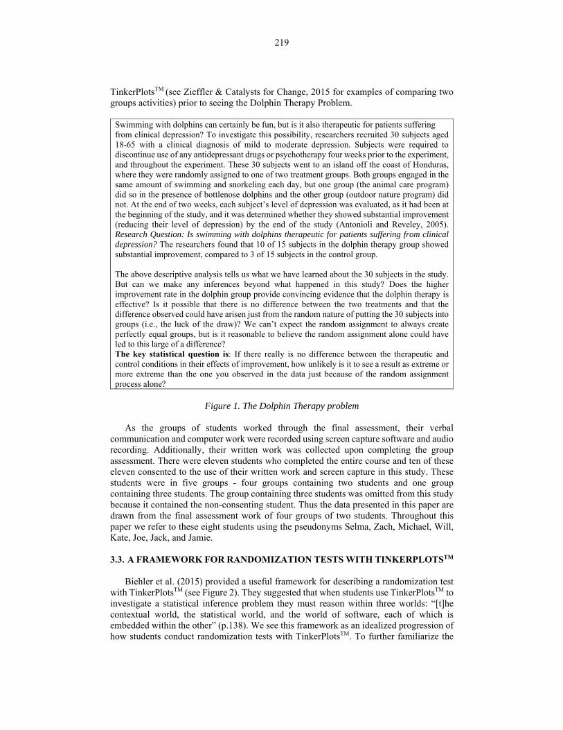
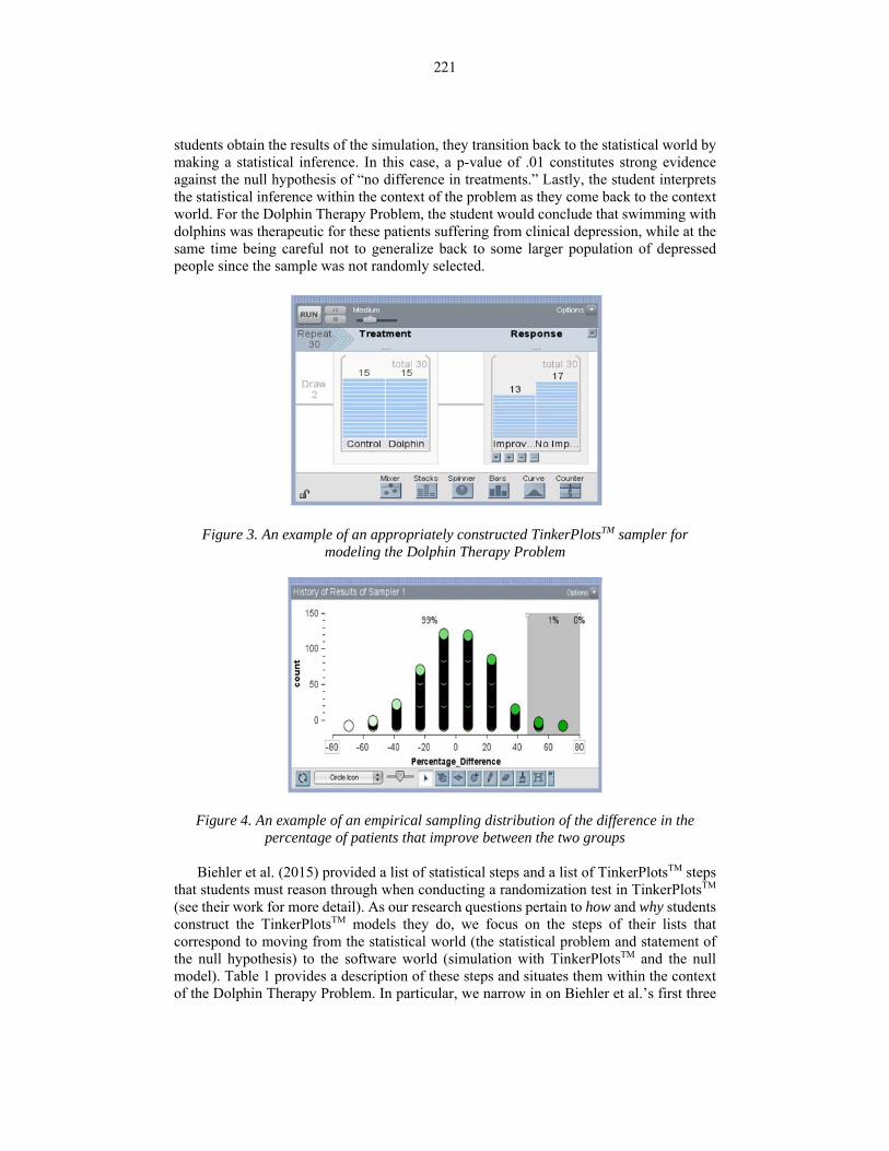
Therapy problem, the context provides the student with the real problem, namely: Is swimming with dolphins therapeutic for patients suffering from clinical depression?. Students then transition into the statistical world by generating a null hypothesis. Here the appropriate null hypothesis would be: There is no difference between dolphin therapy and control therapy in their effects on depression. Students further reason within the statistical world by selecting an appropriate statistical test. Since the Dolphin Therapy Problem describes the random assignment of patients into treatment groups, an appropriate statistical test would be a randomization test. The null model serves as a link between the statistical and the software world as students use the null hypothesis to construct an appropriate sampler in TinkerPlotsTM and simulate data to answer the research question. A TinkerPlotsTM sampler can be constructed similar to the sampler shown in Figure 3 (or one isomorphic to it). This sampler can be used to generate data and to create an empirical sampling distribution of the difference in the percentage of patients that improve between the two groups (see Figure 4). Using the observed difference in the percentage of patients that improve between the two groups, 46.7%, a p-value of 1% can be found using the divider feature in TinkerPlotsTM (as indicated by the shaded region in Figure 4). Once

221

students obtain the results of the simulation, they transition back to the statistical world by making a statistical inference. In this case, a p-value of .01 constitutes strong evidence against the null hypothesis of “no difference in treatments.” Lastly, the student interprets the statistical inference within the context of the problem as they come back to the context world. For the Dolphin Therapy Problem, the student would conclude that swimming with dolphins was therapeutic for these patients suffering from clinical depression, while at the same time being careful not to generalize back to some larger population of depressed people since the sample was not randomly selected.

Figure 3. An example of an appropriately constructed TinkerPlotsTM sampler for modeling the Dolphin Therapy Problem

Figure 4. An example of an empirical sampling distribution of the difference in the percentage of patients that improve between the two groups

Biehler et al. (2015) provided a list of statistical steps and a list of TinkerPlotsTM steps

that students must reason through when conducting a randomization test in TinkerPlotsTM (see their work for more detail). As our research questions pertain to how and why students construct the TinkerPlotsTM models they do, we focus on the steps of their lists that correspond to moving from the statistical world (the statistical problem and statement of the null hypothesis) to the software world (simulation with TinkerPlotsTM and the null model). Table 1 provides a description of these steps and situates them within the context of the Dolphin Therapy Problem. In particular, we narrow in on Biehler et al.’s first three

222

TinkerPlotsTM steps. We conjecture that these first three steps are crucial to really understanding statistical inference from a modeling and simulation perspective. We also consider how students’ interpretations of the null hypothesis given in the Dolphin Therapy problem influenced their reasoning when translating the null hypothesis into a simulation model in TinkerPlotsTM (translation from null hypothesis to null model is the third statistical step in Biehler et. al). In translating the null hypothesis into a null model in TinkerPlotsTM, determining what to select as the ratio of the two outcomes in the sampler device and whether to set the device to with or without replacement are not trivial problems. Solutions require an understanding of what is happening in TinkerPlotsTM when the simulation runs, what assumptions can be made about the groups, and whether the inferences can be drawn with respect to some larger population or if inferences are causal.

Table 1. Selected steps for conducting a randomization test as described by Biehler et al. (2015, p. 147). The third column describes the Dolphin Therapy Problem in terms

of these steps.

Steps Described by Biehler et al. (2015) Description of Steps Dolphin Therapy Problem

Statistical Step – Describing the Null Model

“The null hypothesis then has to be translated into a simulation model in TinkerPlotsTM. The simulation model needs to include a sampler device for each attribute” (p. 144). This step represents a transition from the statistical world to the computer world.

Null Hypothesis: There is no difference between dolphin therapy and control therapy in their effects on depression. Translation to Null Model: A linked device containing two samplers. Each sampler device should contain a total of 30 elements (people). The first sampler attribute labeled “Group,” contains two outcomes titled “Dolphin” and “Control” (15 for each outcome). The second sampler attribute labeled “Response,” contains two outcomes titled “Improve” (13) and “No Improve” (17). Both devices set to without replacement. We want to think of the sampler devices as randomly allocating a person from one of the therapy groups to a result of improved or not improved and repeating this process until all 30 patients have been allocated a result at random. This random shuffling of group to outcome allows us to see if chance alone could produce the outcomes reported in the original experiment.

TinkerPlots

Step 1 (TP1)

Populating the mixers with the correct labels/values to mimic the original sample (p.148).

In the Dolphin Therapy Problem that would mean constructing two linked devices that can be set to with or without replacement. One device is for the “Group” attribute (15 “Dolphin” and 15 “Control”) and one device is the “Response” attribute (13 “Improved” and 17 “Not Improved”). Draw is automatically set to 2 since we draw one element from the “Group” attribute and assign it at random to an element drawn from the “Response” attribute.

TinkerPlotsStep 2 (TP2)

Setting the number of repetitions (how many cases should be randomly selected

Biehler et al. suggest this step is about how to set the Repeat. For the Dolphin Therapy problem this

223

from each mixer) to the original sample size (p. 148).

would mean setting Repeat to 30 since there are 30 patients in the study.

TinkerPlotsStep 3 (TP3)

Setting the number of repetitions (how many cases should be randomly selected from each mixer) to the original sample size (p. 148).

Biehler et al. suggest this step is different than TP 2 and relates to whether the devices are set to with or without replacement. Both devices are set to without replacement. We want to keep the numbers of those in the “Dolphin” and “Control” groups the same with each run of the simulation (exactly 15 for each group) and we want to keep the overall patients that improved and did not improve in the same ratio of 13 to 17. This allows us to create the random allocation of “Group” to “Response.”

TinkerPlotsStep 4-7 (TP4-TP7)

Plotting the randomized sample and depicting the measure of deviation Collecting the chosen measure from many different re-randomizations Plotting the collected statistics Computing the p-value

Running the TinkerPlotsTM model. Plotting the outcomes “Dolphin”/”Control” and “Improve”/”No Improve.” From here the percentage difference in patients that improved between Dolphin Therapy and Control group can be calculated. Collecting statistics and creating a sampling distribution on the percentage difference.

3.4. DATA ANALYSIS

We view the framework and subsequent statistical and TinkerPlotsTM steps outlined

by Biehler et al. (2015) as a concrete approach that suggests a way to operationalize modeling and simulation problems with TinkerPlotsTM. By breaking down the Dolphin Therapy Problem into discrete statistical and software steps, we have both a way to share a normative approach to the problem as well as a method for assessing student work. Their framework and steps also provided us with an approach to data analysis in our research.

Our analysis was multifaceted. Both authors independently reviewed the video and transcripts from the video sessions of the four consenting groups, focusing on students’ reasoning. We honed in on the models students created and how they discussed the various features (i.e., Draw, Repeat, with or without replacement, attribute labels, as well as how they were populating their samplers) of their models. While independently reviewing the video tapes, each author took notes and highlighted what they saw as important aspects of each group’s model construction. We then came together to discuss our initial notes and summaries. We looked for areas of agreement and disagreement, discussing any disagreements until we reached consensus.

The steps of Biehler et al. (2015) helped us pinpoint places in student transcripts for further investigation by identifying which steps students tended to struggle with. We reviewed the qualitative aspects of student responses, their justifications for the various features of their models, to better understand why students set their models up the way they did. We also noted any places in students’ discussions where they explicitly attempted to relate their null hypothesis to their TinkerPlotsTM model. Biehler et al. discussed this as the null model and indicated that it is an important transition from the statistical world to the software world. This helped us identify places where students appeared to be explicit about the translation from the statistical world to the software world. Through this iterative process of independent review followed by discussion and consensus seeking, as well as applying the framework of Biehler et al. as a way to organize our data analysis efforts, we identified important parts of students’ discussions where they addressed the various features of their TinkerPlotsTM models and where they made explicit connections between the null hypothesis and their models. We highlight these places in our results section and

224

offer some characterizations of student thinking during the TinkerPlotsTM model construction phase.

4. RESULTS

In this section we share the results of four groups of two students (Selma and Zach – Group 1; Michael and Will – Group 2; Kate and Joe – Group 3; Jack and Jamie – Group 4). Excerpts presented here are organized around the research questions presented at the beginning of the paper. The reader may notice that there is considerable overlap between students’ responses when connecting the null hypothesis to the TinkerPlotsTM model (i.e., Research Question 1) and when describing specific aspects of the TinkerPlotsTM model (i.e., Research Question 2). From our perspective this overlap is expected since students consider these aspects of the TinkerPlotsTM model when attempting to articulate their null hypothesis into a model in TinkerPlotsTM.

Primarily results pertain only to students’ work setting up and reasoning about their models. In some instances, excerpts of a group’s work after their TinkerPlotsTM model set-up are shared. These instances highlight cases where the output from running their model caused them to go back and make changes to their original model. We add italics to places in the transcripts where the evidence of students attempting to justify features of their models or relate them back to the null hypothesis appears particularly strong. 4.1. RESEARCH QUESTION 1 (CONNECTING THE NULL HYPOTHESIS TO

THE TINKERPLOTSTM MODEL) Selma and Zach (Group 1) did not change their model over the course of their work

(see Figure 5).

Figure 5. Group 1’s TinkerPlotsTM model for the Dolphin Therapy Problem

They constructed a linked device model. The first device contained the “Treatment” attribute (15“Dolphin”/15“Control”). This device was set to without replacement. The second device contained the “Response” attribute (13“Improve”/17“Not Improve”). This “Response” device was set to with replacement. Draw was set to 2 and Repeat was set to 30.

Zach summed up the relationship between the null hypothesis and their TinkerPlotsTM model.

225

Zach: Our model represents that because, we should get an equal distribution of improvement in both the control and the – with this model we should get an equal amount of improvement in both the dolphin and control group.

Mike and Will (Group 2) constructed a model isomorphic to that of Selma and Zach.

See Figure 6 for a visual representation of their TinkerPlotsTM model.

Figure 6. Group 2’s TinkerPlotsTM model for the Dolphin Therapy Problem

Mike and Will also did not change their model over the course of their work. The excerpts below show their consideration of two types of statistical tests, randomization or bootstrap, as they initially set up their model.

Will: Okay. What kind of model do you think we should use to do these? We’ve got the randomization and the bootstrap.

Mike: Randomization test. Will: Well bootstrapping I believe is when you have – when you don’t have as many results

versus the populous. Mike: Mmm, okay. Yeah, yeah, yeah. Will: And if we are talking about the population being people who suffer from clinical

depression… that’s a pretty significant population. Mike: Yeah. Will: So we might want to do bootstrapping. Which I think, if I remember the only

difference from that is that you, umm, the potential results versus depressed and not depressed can be re-selected.

Will steered his groupmate toward the bootstrap in this discussion. In particular, he

discussed wanting to relate any results back to a larger population of all depressed people and that by re-selecting or using the bootstrap they may be able to say something more about the general population. After this initial conversation the instructor came over to check on this group’s progress. During the conversation with the group the instructor inquired as to whether the study was experimental or observational, to which Will responded, “This is an experiment...So you would suggest using the randomization?” While the instructor did not provide Will with a response to this question, she did ask some additional questions about what kinds of inferences could be drawn in this study and what a significant result might indicate. The students’ initial inclination to generalize to the population persisted throughout this discussion and ultimately they concluded that a

226

bootstrap would allow them to make comparisons to the larger population of depressed people.

Will: I think that the bootstrap is okay because we are comparing it to the whole population of people who have clinical depression.

Mike: Mhmm. Will: And the bootstrap allows a greater variance for potential variability. Mike: Yeah. Will: Uh, as opposed to just permuting what we got in the study itself.

Whereas Group 1 discussed the equal distribution between groups when relating their

TinkerPlotsTM model back to the null hypothesis, Group 2 appeared to relate results back to a larger population of depressed people rather than “just permuting what we got in the study itself.” This statement indicated that they saw the difference between a bootstrap and randomization test. In addition, an earlier comment suggested they knew that randomization tests can be used with experiments - when the instructor asked them if the study was an observation or experiment.

Groups 3 and 4 share some similarities in the approaches they took and the struggles they had. Kate and Joe (Group 3) created two different models over the course of their work on the Dolphin Therapy Problem. Their first model is the correct model (see Figure 7). They set up a linked device model where the first device contained the attribute “Groups” and the second device contained the attribute “Improvement.” They set both devices to without replacement. In addition, both devices were populated with the correct values from the original sample.

Figure 7. Group 3’s first TinkerPlotsTM model for the Dolphin Therapy Problem

Kate and Joe did not keep the first model they created for very long. After they set up the model in Figure 7, Kate ran a single trial and began to plot the results of “Improve” and “Not Improve.” Immediately she re-read the problem and suggested changing their model to a 50/50 model (see excerpt below). The group changed their model in the following way: they changed the values in the “Improvement” attribute so that there were equal numbers for the “Improve” and “Not Improve” outcomes (15/15), see Figure 8 for their second model.

227

Figure 8. Group 3’s second TinkerPlotsTM model for the Dolphin Therapy Problem

The excerpt below is the discussion that lead them to modify their model.

Kate: Hold on. So it says [she re-reads the problem out loud] if there really is no difference between therapy treatment how likely it is that you would see a result as extreme or more extreme than the one you observed in the data... So it should be fifty-fifty [Improved/Not improved]. This should be fifty-fifty.

Joe: The improvement. Kate: Yeah. Joe: Why? Kate: Because this model is supposed to represent the null hypothesis. Joe: Okay. Kate: This model is supposed to represent the conception that there is no difference.

This was a pivotal point in this group’s model development. As Kate re-read the

problem and attempted to connect their TinkerPlotsTM model to the null hypothesis she focused on constructing a model that represented a null hypothesis of “no difference.” However, she interpreted “no difference” at the person level - as a person it is just as likely to improve as not improve.

Finally, Kate shared her thinking with her partner about the connection between the null hypothesis and the TinkerPlotsTM model.

Kate: We used stacks to represent therapy groups and possible outcome of choices. The model represents the null hypothesis in that it gives equal chance for each patient to either receive an improvement or no improvement outcome which assumes there is no difference between the effectiveness of the therapies.

Kate wanted to give each patient an equally likely chance of improving or not

improving and she appeared to equate or connect this with the idea of equal improvement at the group level because she went on to say that this assumes “no difference between the effectiveness of the therapies.” Without instructor intervention it is likely that this group would have kept this 50/50 model as their final model for the Dolphin Therapy Problem. The next excerpt shows the conversation between the instructor and the students.

Instructor: Is saying there is no difference between the two therapies the same as saying equally likely?

Kate: Okay so we should have described it the way we did before?

228

... Instructor: …tell me what is the difference setting both groups up as fifteen-fifteen for

dolphins and fifteen-fifteen for improve/no improve versus the seventeen-thirteen no improve/improve. … Can you articulate to me the difference?

... Kate: Okay so this is like the smoker thing [referring to a previous comparing two groups

activity that used randomization techniques called Social Fibbing (see Zieffler & Catalysts for Change, 2015, p. 203)]. In this, the way we have it now (50/50 model) is like having the spinner set at fifty-fifty so assuming no differences between the therapies. That the Dolphin therapy is just as effective or ineffective as being in nature without dolphins. But if we set to seventeen-thirteen that would be when we simulated if it’s as equally likely as the no dolphins to be as effective. Because it would randomly match it, right? So it could be potentially as no dolphins could be as effective as dolphins.

The instructor questioned Kate’s connection between 50/50 for the outcomes

“Improve” and “Not Improve” and the null hypothesis of no difference between the two therapies. But it’s unclear from Kate’s response that she saw a distinction, only that she responded to the instructor’s questioning by assuming her group’s current model must be wrong. The discussion continued with the instructor attempting to get the group to articulate the differences between the two models they created. Kate attempted to articulate the differences suggesting that a fifty-fifty spinner is “assuming no difference between the therapies” and that seventeen-thirteen is simulating “if it’s (Dolphin Therapy) equally likely as the no dolphins to be as effective.” Her responses appeared to be equivalent, suggesting that the distinction between the two models is not entirely clear to her.

Group 3 did change back to their original model (see Figure 7) but there was no further discussion and no evidence to suggest that they understood the random assignment in their model or how it related to the null hypothesis. What does seem clear from their discussion was that to them setting the “Improvement” sampler to 15/15 for the outcomes “Improve” and “Not Improve” translated to a null hypothesis of no difference between the two therapies. That is, they did not appear to see a true distinction between a statement of no difference between the two therapies and a statement that a person is just as likely to improve or not improve.

Group 4’s confusion was similar to that of Group 3. They both created models that gave an equally likely chance for a patient to improve or not improve. The next excerpt shares Group 4’s initial thinking as they attempted to create a TinkerPlotsTM null model to model the null hypothesis.

Jack: So the null model assumes that... Jack and Jamie: There is no difference. Jack: I guess for this model should we do two samplers that are showing like

improvement versus no improvement or should we just do one sampler that... the percentage of improvement between the two.

Jamie: Okay so the null model would say that there is no difference in improvement. Well there's no diff - dolphins won't help compared to other….So we would need fifteen and fifteen. Yeah.

... Jack: Should they be equal? Jamie: They should be equal because um each person would have an equ... ... Jamie: Like the null model would say that each person has a, just as likely a chance

of improving or not improving no matter what group they are assigned to.

229

Jack: Okay so why don't we just do spinners, I guess. …Like there's a fifty-fifty percent chance that they'll improve if they want to improve.

In this excerpt Jack and Jamie worked to create a TinkerPlotsTM model based on their

null hypothesis. Initially they talked through what that assumption was – “no difference,” they both stated this simultaneously. Jack suggested the null model means there’s no difference in improvement “between the two,” and Jamie said if there’s no difference than “dolphins won’t help compared to the other.” Jamie also stated that “each person has just as likely a chance of improving or not no matter what group they’re assigned to.” Jamie’s excerpts seem to suggest that she has conflated “no difference” at the individual level, for example where she suggested each person has just as likely a chance of improving, with no difference at the group level, for example where she suggested it does not matter what group they are in. The dialogue in these excerpts suggested a struggle to understand where “no difference” should figure into the model. The model they created was also consistent with a null hypothesis where no difference in improvement is at the individual level. That is, a person has an equally likely chance of improving or not improving.

This group created two linked spinners. The first spinner’s attribute was labeled “Control Group.” The second spinner’s attribute was labeled “Dolphin Therapy Group.” Each spinner was split into two equal parts with one part labeled “Improvement” and the other part labeled “No Improvement.” Their TinkerPlotsTM model is shown in Figure 9.

Figure 9. Group 4’s first TinkerPlotsTM model for the Dolphin Therapy Problem It is likely that this would have been the final model for this group except that the

instructor intervened and asked them about their model.

Jack: So we just chose to do a spinner with equal values since there would be no chance between the two.

Jamie: The null methods would say that... Jack: There's no difference. Jamie: There's no difference between cont - Like the dolphins won't help. Instructor: Does saying that there's no difference between the control improving and the

dolphin group improving, which you are saying is the null model, mean the same thing as saying they’re equally likely to have improvement? That everyone is equally likely to have improvement?

Jack: I'm wondering now if we just needed one model, one spinner that had... Jamie: Improvement or not improvement?

230

The group’s response to the instructor’s initial question suggests they struggled with how to connect the statistical null hypothesis to the TinkerPlotsTM null model. The instructor then asked the group to think back to several of the activities on comparing two groups that were done in previous class work. After she asked them to reflect on these activities, the following discussion ensued.

Jamie: I'm still not sure if we are simplifying it or over complicating it. Jack: I think we’re simplifying it too much. …we could have two stacks that's fifteen

people from the dolphin therapy and fifteen from the control group and then have another stack that's how many people improved versus how many people didn't improve.

Jamie: And pair them up? Jack: And seeing what the difference is. Jamie: So like one stack with 30 people getting paired up with whether... Jack: They improved or not. Instructor: So how does that represent the no difference model? Jack: Because that would show that they are equally likely to report or whether or not like

based off the data that we have or not.

In this last excerpt Jack and Jamie began to revise the group’s current model by creating one attribute for “Group” and the other attribute for “Response” (as opposed to having one attribute for “Dolphin” and one attribute for “Control” as their initial model contained). They appeared to go in this direction based on thinking back over previous classroom activities that utilized randomization tests. However, when the instructor asked how their description of this new model represented the “no difference” model, Jack struggled to adequately articulate the idea of randomization.

Jack: So I was thinking based off that smoking thing [referring back to a prior comparing two groups problem that utilized a randomization test], if we had two stacks both with fifteen...

Jamie: So one's dolphin and one’s control [changing the stacks device to 15/15 Dolphin/No Dolphin for the first attribute.]

Jack: Then having this other stack... Jamie: Which would be seventeen and thirteen? Jack: Yeah. Thirteen people improved and seventeen people didn't improve and then doing

without replacement and without replacement [on both devices] and then doing that thirty times. And seeing like so there's always an equally likely chance of that happening. I don't know though if. Yeah so I think that makes sense. I just can't explain it well enough.

At the end of this excerpt Jack tried to explain the null hypothesis in terms of the model

but still struggled to describe the idea of random assignment. The students did not appear able to describe the process that occurs when the sampler was run. Figure 10 shows the model they constructed based on the previous excerpts.

231

Figure 10. Group 4’s second TinkerPlotsTM model for the Dolphin Therapy Problem; the red circles were added to highlight that the group did not change the attribute names, and the red circle around Repeat is to highlight that they started with 30 but quickly

switched to 15

This group’s model, shown in Figure 10, was essentially correct except their attribute labels were incorrect. This will be discussed further in the next section when we address attribute labels. The group tried to discuss the connection to the null hypothesis by saying this model “gave both groups an equally likely chance of reporting whether or not they improved based off the data from the experiment,” but this description avoided actually discussing random assignment. They discussed “equally likely” instead of “no difference” and they suggested the “equally likely” is represented by using data from the experiment. Their description of connecting the null hypothesis to their TinkerPlotsTM model appeared more confused than it did when they described the connection to their first model (see Figure 9). The instructor came back to this group and pressed them on their reasoning once more. At this point the group revealed the fragility of their thinking about how the null hypothesis connected to the TinkerPlotsTM null model.

Instructor: When you say equally likely for someone to improve as not improve or that it’s equally likely…

Jamie: That one person from a group is going to report improvement or not improvement. That it’s just as likely that someone from the control group is going to report improvement as someone from the dolphin group. … Set to without replacement because once an observation is picked we don't want it to go back in there and have possibility of getting picked again.

Instructor: So why thirteen-seventeen versus fifteen-fifteen? Jamie: Because of the data they gave us. Jack: Because we would just get the same result. Because each time we'd always get

fifteen people. Actually I don't know, maybe not. Maybe that would have been better?

Jamie: The thirteen-seventeen is showing us a model where there is a difference and don't we want to try to model that there isn't a difference.

When the teacher pressed this group about the null hypothesis of “no difference

between therapies” and the relationship to the TinkerPlotsTM model, it revealed the fragility of their understanding. Initially Jamie suggested the new model shows it’s just as likely to report improvement from the control group as from the dolphin group. But then when asked

232

why 13/17 versus 15/15, Jack said that 15/15 may be a better option and Jamie suggested that 13/17 shows a model where there “is a difference.”

4.2. RESEARCH QUESTION 2A (ATTRIBUTES, DRAW, POPULATING THE

SAMPLER)

Students’ decisions on labeling attributes, their justifications for Draw and their choices for how to populate the sampler correspond to Biehler et al.’s (2015) TP Step 1. Students did not spend much time discussing attribute labels or what type of devices they wanted to use. Group 1 spent a bit more time than the other groups deciding on the labels for their attributes, going back to the problem context to re-read the language used, but we do not have evidence that labeling attributes was in any way problematic in and of itself. However, evidence from Group 4 suggests that poor labeling of attributes can create problems for other aspects of the modeling process. Group 4 changed their model (recall analysis in the previous section), but when they changed their model, they neglected to re-label their attributes (see Figure 10). This created challenges for how they determined their Repeat value. This issue is examined in the next section.

Draw appeared to occupy very little time in terms of student discussion. In fact, because of the way TinkerPlotsTM is configured, Draw is already set at 2 for the students as soon as they create a linked device – one element is drawn from each device. Thus students did not have to decide on a value for Draw, rather they had to justify the reason why it was 2. We share a brief excerpt for Kate and Joe (Group 3), as this is very similar to how other groups justified a Draw value of 2.

Joe: For draw we had two. What were the two groups called? Kate: One to pick from the two therapy groups and one to pick whether or not they

improved. So each patient is matched with a result.

Students’ choices for how to populate their samplers appeared to be inextricably linked to how they connected the null hypothesis to their TinkerPlotsTM models. Evidence from section 4.1 revealed how each group constructed their TinkerPlotsTM models. All four groups populated the “Group” attribute with 15 “Control” and 15 “Dolphin” Groups 1 and 2 populated their second device with 13 “Improve” and 17 “No Improve” because they were either interested in maintaining the probability of “Improve” versus “No Improve” with each draw (Group 1) or because they wanted to draw conclusions back to a larger population of depressed people (Group 2). Groups 3 and 4 struggled to correctly populate their sampler devices because they confused “no difference” at the group level and no difference at the patient level. 4.3. RESEARCH QUESTION 2B (REPEAT)

For three of the groups (Groups 1, 2, and 3) deciding what to set Repeat to and why appeared to be relatively straightforward. Mike’s response (from Group 2) is shown below. The responses from the first three groups suggest they attended to the 30 individuals from the study and attempted to replicate that.

Mike: The repeat is set at thirty to simulate thirty individuals.

Group 4 struggled with determining a value for Repeat. This group oscillated between a Repeat value of 15 and of 30. However, the reason for their struggle is complex and relates to how they connected their null hypothesis to the TinkerPlotsTM model they

233

constructed and how they labeled their attributes. Recall from the previous section that this group did not re-label the attributes they used from their first model (Figure 9) when they created their second model (Figure 10), resulting in attribute titles that no longer made sense with their new model. After they ran the simulation using their second model, Jamie and Jack lost focus on the relationship between the TinkerPlotsTM model and the null hypothesis and re-focused their thinking on Repeat. They ran the simulation on the model shown in Figure 10 and constructed a plot of “Improvement” versus “No Improvement” (see Figure 11). They became confused when they realized the counts for these two outcomes summed to 30 (recall that each group consisted of 15 individuals). Since they did not re-label their sampler attributes, they saw these as counts for the “Dolphin Therapy Group” only. The second device’s attribute really represented “Responses” in their second model – total number of patients that improved and did not improve.

Figure 11. Group 4’s plot of a single trial after running their new model. The red circles are meant to highlight the counts for both outcomes as well as the attribute name that the

group previously did not correct. The following excerpt highlights the group’s confusion as they grappled to understand

why they were seeing 30 patients in the “Dolphin Therapy Group.”

Jack: Is this the right thing? It should have been fifteen? [Referring to Repeat]. Right? Jamie: No it should have been thirty? Jack: …Because it’s only supposed to be fifteen from each group? Jamie: But it should take one from here and one from here and match them [Referring to each

stacks device]. Jack: Why is it not, why is it doing? …That's so weird, but I'm just wondering, like, why it’s

showing that way [He makes a plot of improvement and not improvement for dolphin group and they count the totals and they see 30 total, see Figure 11].

Jack: It should only be fifteen from each trial because that will give us more results than we want. So maybe it [Repeat] should be fifteen.

Jamie: Should it be fifteen? Jack: Yeah [he changes the Repeat to 15 and then plots again and sees 15 in the total for

their graph counts].

Neither Jack nor Jamie noticed the naming of the attribute issue and in order to get only 15 in the counts for their plot (see Figure 11) they changed Repeat from 30 to 15 (changing the Repeat value in Figure 10 to 15). However, when the instructor came back and asked them to explain their thinking the group then realized the need to rename the attributes.

234

They re-labeled their attributes, “Group” and “Result.” Then they ran their model (see Figure 10, but with re-labeled attributes and with Repeat set to 15). Once they ran this model they revisited Repeat values of 15 versus 30 again. Finally, when they plotted “Results” after running a single trail, Jack noticed their new plot only contained 15 people and he wanted to know why they did not have 30 anymore. They quickly solved this by adjusting Repeat to 30. Group 4’s final model is shown in Figure 12.

Figure 12. Group 4’s final TinkerPlotsTM model for the Dolphin Therapy Problem 4.4. RESEARCH QUESTION 2C (WITH OR WITHOUT REPLACEMENT)

Group 1 set up the first device to without replacement and their second device set to with replacement (see Figure 5). Initially Zach suggested both devices should be without replacement, but Selma convinced him that the second device should be set to with replacement.

Selma: We want to keep the probability so that’s (pointing to “Response” attribute) with replacement, right?

Zach: Without. Selma: No cause if you keep it with replacement then it goes back into the bucket. Zach: Mmhmm. Selma: Does that make sense? So we have like one bucket with like one green candy and one

red candy and we take out one red candy then your percent of getting green, it now changes. It’s no longer fifty it is now one hundred.

Zach: You’re right. …

Selma: So the first device for the type of treatment will be simulated without replacement. Zach: Right. So that um we get exactly fifteen in control and fifteen in dolphin group. And

the second device is the response. Selma: The second device is the response attribute, which we’ll simulate with replacement to

maintain the probability of improvement versus non-improvement within the experiment.

Selma wanted the “Response” attribute to maintain the same probability after each

draw (in order to keep the same ratio of 13 “Improved” to 17 “Not Improved”) and thus, they wanted to set the device to with replacement. She used two colors of candy in a jar to help clarify her idea to her partner.

235

While Groups 1 and 2 constructed isomorphic models (see Figure 5 and Figure 6, respectively), they appeared to have very different reasoning for setting their “Response” device to with replacement. Group 1 wanted to maintain the same probability of “Improve” and “Not Improve,” whereas Group 2 wanted to make generalizations back to a larger population of depressed people (recall work presented by Group 2 in section 4.1). In addition, Group 2’s final write up stated:

The replacement for the group sampler is set at without replacement because we do not want each draw to replace the value. The replacement for the result group is set at with replacement. It is important to note that we conduct this model as a bootstrap in order to simulate the variability of the overall depression population. We want to simulate a greater degree of variability in the null model. Groups 3 and 4 set both of their devices to without replacement (see Figure 7 and Figure

12, respectively). Both of these groups constructed their final models by recalling a previous randomization activity they had seen in class. But there is no evidence from either of these groups that they understood that setting their samplers up in this way created the random allocation of treatments to responses, rather they appeared to be relying on their memory of the sampler set up from the previous activity.

5. DISCUSSION

The discussion section is also organized around the research questions posed at the beginning of the paper and relate this work back to the first three TinkerPlotsTM steps described by Biehler et al. (2015) and their framework for solving comparing two groups problems. 5.1. RESEARCH QUESTION 1: NULL HYPOTHESIS AND THE CONNECTION

TO THE TINKERPLOTSTM MODEL The null model as described by Biehler et al. (2015) is the transition from a student’s

statement of the null hypothesis (statistical world) to the TinkerPlotsTM model, the random device (computer world). Our students were essentially given the statement of the null hypothesis in the problem because they were asked if there really is no difference between the therapeutic and control conditions in their effects of improvement, how unlikely is it so see a result as extreme or more extreme than the one you observed in the data just because of the random assignment process alone? However, these groups created different models or had different reasoning about connections between their TinkerPlotsTM model and the null hypothesis. Group 1 seemed most able to articulate this distinction when Zach stated, “We should get an equal distribution of improvement in both the control and the – with this model we should get an equal amount of improvement in both the dolphin and control group.” Group 2 did not explicitly discuss the relationship between the null hypothesis of “no difference between groups” to their TinkerPlotsTM model, rather they focused on making generalizations back to a larger population. Groups 3 and 4 created models that included an additional assumption that a person was equally likely to “Improve” or “Not Improve.” These groups appeared confused between no difference at the group and individual levels. This suggests that the concept of no difference between two groups is difficult to operationalize into a TinkerPlotsTM model. For these groups it was more challenging to see the random assignment as creating “equal groups” or an “equal distribution of improved and not improved between the two groups,” rather than a model that creates the same likelihood that a patient improves or does not improve. It may also be a general confusion about the actual randomization process happening in TinkerPlotsTM

236

when the model is run. That is, perhaps for these students the software acted as a black box in which they simply input information. 5.2. RESEARCH QUESTION 2A & TINKERPLOTSTM STEP 1

TinkerPlotsTM Step 1 includes determining which devices to use (devices that can be

set to with or without replacement), how to populate the devices (what values go into each outcome for each attribute) and how to label the attributes. In this section we discuss two key findings related to students’ reasoning with aspects of the TinkerPlotsTM model in Step 1 - naming of the attributes and populating the devices.

When describing TinkerPlotsTM Step 1, Biehler et al. (2015) asserted that it is not necessary to rename the attributes on the sampler and that it was not essential to correctly modeling a comparing two groups problem using randomization. However, in our study we found that the naming of attributes was actually important for students. Specifically, Group 4 ran into problems when they changed their initial model but did not re-label their attributes to match the changes made to their model. Since their devices fundamentally changed from each device representing a “Group” to the first device representing the “Group” attribute and the second device representing the “Response” attribute, it was imperative for them to re-label or mentally track the interpretation of the attribute during their simulation. However, this group did not initially re-label their attributes and as a result they made errors in setting the value of Repeat. They thought their 30 outcomes of “Improve” and “Not Improve” were all results from one group, “Dolphin Therapy Group.” This error lead them to change their Repeat value to 15. We argue that the naming of the attributes is an important aspect of the modeling process. For example, the names students give to the attributes can serve as a bridge (or concrete component) between the context world they began in and the more abstract world of the computer within which they are trying to build their model. When they run their simulation and build plots, those attributes become the titles on the axes of their plots and give meaning to how they read and interpret those plots.

Students’ choices for how they populated their devices varied. Two of our groups (Groups 3 and 4) made one of the “mistakes” identified by Biehler et al. (2015). Our work gives more insight into why students may be inclined to populate the “Response” attribute device with an equal number or ratio of “Improve”/“Not Improve.” Groups 3 and 4 both struggled with how to populate the “Response” attribute and had strong inclinations to create models that contained an equal number or ratio of “Improve” and and “Not Improve.” Their reasoning for this choice was directly related to how they connected the null hypothesis to the TinkerPlotsTM model they were constructing. These two groups articulated a null hypothesis of “no difference between the two groups,” but their models suggested a null hypothesis that included the additional assumption that each person had an equally likely chance of improving or not. There needs to be a distinction in students’ minds between equal chance for improvement in patients versus an equal chance for improvement between the two therapies. When questioned by the instructor, these two groups struggled to tease apart a clear distinction between “no difference” at the group level and the patient level. We have four conjectures as to why this 50/50 model may be appealing to students.

First, it is possible that Groups 3 and 4 lacked an understanding of the process of random assignment in this context and perhaps did not understand what a randomization model in TinkerPlotsTM does once Run was clicked. That is, there is no evidence that these students imagined the process of permuting “Group” to “Response”. They used the

237

language of “matching” patients with results. We suspect more explicit discussion about how to interpret the process happening in TinkerPlotsTM when a model is run is necessary.

Second, it is possible that Groups 3 and 4 either conflated or equated the idea of no difference between the therapy groups and the idea that a person is just as likely to improve or not improve. Their language throughout the excerpts blur these two ideas and a few times they simply used the phrase “no difference.” It is likely that both groups would have kept their first model without intervention from the instructor and they struggled to articulate distinctions between no difference at the group and patient levels in their models.

Third, it is worth noting that at times the students from Groups 3 and 4 automatically shortened their statement about the null hypothesis to simply “no difference.” On the one hand, the curriculum has clear statements with respect to the null hypothesis. For example, statements such as “assuming there is no difference between conditions in their effects…” (Zieffler & Catalysts for Change, 2015, p. 128, italics in the original). On the other hand, the materials emphasize “no difference.” The curriculum also emphasizes the model as the “just-by-chance model.” It seems clear that the emphasis on “no difference” (or “just-by-chance”) in the null hypothesis statement is a pedagogical choice designed to help students by expressing a complicated idea in fewer words. However, it may also hinder students if they cannot explicitly see where the “no difference” or “just-by-chance” presents itself when translated into a TinkerPlotsTM model. Noll and Hancock (2015) explored how language can mediate students’ statistical problem solving activities and how expressing new ideas in fewer words can both help and hinder student learning. We conjecture that the emphasis on the shortened phrases of “no difference” or “just-by-chance” with respect to the null hypothesis may act in ways that hinder students’ ability to adequately relate where the “no difference” can be mapped to the TinkerPlotsTM model and may lead to possible confusion between “no difference” at the group or individual level. It would be worthy of future research to investigate these ideas.

Fourth, a 50/50 model might appeal to students due to the influence of one-population problems on student thinking when they begin comparing two groups. In the first unit of the CATALST curriculum, students encounter problems in which the appropriate TinkerPlotsTM model is a 50/50 spinner (or stacks or mixer). For example, in one problem in the curriculum students are told about a study in which infants are observed selecting a “helper” toy or a “hinderer” toy. They are told that 14 out of 16 randomly selected infants chose the helper toy and asked if this result could be considered unusual if children really have no preference for toy type (For a closer look at the Helper or Hinderer Activity see Zieffler & Catalysts for Change, 2015, p. 61). The null hypothesis then is that infants have no preference for the helper or hinderer toy and the corresponding TinkerPlotsTM model should include a sampler device, such as a spinner, where 50% is assigned to “helper” and 50% is assigned to “hinderer.” Students work through many problems like this during the first unit and a common initial “mistake” students make when modeling these one-population problems is to use the observed data in the problem when constructing their TinkerPlotsTM model. For example, a student constructs a single device model with two outcomes “helper” and “hinderer” and assigns 14/16 to the “helper” outcome and 2/16 to the “hinderer” outcome (see Noll and Kirin, 2016 for additional examples). Thus, students may be confused when they move to comparing two groups because the modeling process looks very different from these one-population problems. 5.3. RESEARCH QUESTION 2B & TINKERPLOTSTM STEP 2 (REPEAT)

238

TinkerPlotsTM Step 2 relates to determining Repeat. Selecting the Repeat value appeared to be straightforward for students. Also, students appeared to view the Repeat value correctly, as a representation of how many people participated in the experiment – a total of 30. For example, Group 1 created two linked devices (which automatically sets Draw to 2) and suggested Repeat 30 so that they could “pick a therapy group and an outcome for all 30 patients in the study.” The only time this seemed to cause confusion was in Group 4 (Jack and Jamie) but this had more to do with the way they named their attributes, see discussion in section 5.2. 5.4. RESEARCH QUESTION 2C & TINKERPLOTSTM STEP 3 (WITH OR

WITHOUT REPLACEMENT) TinkerPlotsTM Step 3 relates to determining whether to set the devices to with or without

replacement. Setting the second device in a randomization test to with replacement is one of the “mistakes” that Biehler et al. (2015) noted in their work with pre-service teachers. Two of the groups in our study (Group 1 and 2) made this “mistake” and their discussions when constructing their models provide insight into possible reasons why students may be interested in setting up their sampler device with the “Response” attribute set to with replacement.

In all four group’s final models the “Group” attribute device was set to without replacement and all appeared to justify this choice using similar arguments. For example, reasoning included: “because we want exactly 15 to go to the dolphins and 15 to go to control” (Group 4), or “without replacement because each patient could only receive one result” (Group 1). However, determining whether to set the “Response” device to with or without replacement proved more challenging for students. Groups 1 and 2 set their “Response” attribute to with replacement, but for different reasons. Group 2 clearly wanted to bootstrap and articulated that they wanted to be able to generalize back to a larger population of depressed people. This tendency to reason about sample-to-population inference even when given a problem about experiment-to-causation inference is consistent with findings from Pfannkuch, Budgett and Arnold (2015). Pfannkuch et al. suggest that one reason for this tendency may be that many statistics classrooms focus more time on sample-to-population problems. Perhaps it may be natural for humans to want to make inferences back to a larger population. We suspect that other students may reason similar to that of Group 2 when setting up a bootstrap in a randomization type situation, but more research needs to be done to investigate this conjecture. Group 1 also set their “Response” attribute to with replacement but their reasoning was different. This group articulated the desire to keep the probability the same with each draw – to keep the ratio of thirteen to seventeen consistent with each draw. Yet, we do not have insight into why this was important to this group. More research needs to focus on student reasoning for selecting with and without replacement in a TinkerPlotsTM device. For example, are there contexts for which students may naturally create models that focus on random allocation and other contexts in which students may naturally focus on re-sampling? 5.5. ADDITIONAL FINDINGS

In addition to the two “mistakes” identified by Biehler et al. (2015), we also saw

evidence of another developing approach to constructing a comparing two groups problem in TinkerPlotsTM. Group 4’s original model contained two fifty-fifty spinners with one device labeled as the “Dolphin Therapy Group” and one device as the “Control Group” (see Figure 10). The students justified their choice for having fifty-fifty spinners labeled

239

with “Improve”/ “Not Improve,” however, this group did not fully explain why elected to have one device for “Dolphin” and one device for “Control.” This group investigated treatment groups separately, which, we conjecture, may stem from a desire to simplify a comparing two groups problem to a one-population problem.

Our work also shows that the sampler tool appears to serve as a bridge between the statistical world (the null hypothesis) and the software world (a computer model that generates data under the assumption of the null hypothesis) with the context mediating. Students rarely followed any linear order in solving the Dolphin Therapy Problem and at times they moved back and forth between the three worlds identified by Biehler et al. (2015). Our research indicated that once students began working in the software world the context mediated any translating they did between the statistical world and software world. For example, students went back to the context to (1) consider how to name their attributes, (2) determine a value for Repeat – 30 patients, and (3) to determine with or without replacement. The context helped inform how they constructed parts of their TinkerPlotsTM model and there is a natural movement between each world throughout the problem solving process. Therefore, we would add bi-directional arrows as well as arrows that jump from the context world to the computer world to Biehler et al.’s framework (see Figure 2).

6. CONCLUSION Biehler et al. (2015) rated pre-service teachers as “successful” or “not successful” for

each of the 7 TinkerPlotsTM steps. Success on later steps was not contingent upon success on previous ones. Students’ performance was rated as “good” if TinkerPlotsTM Steps 2, 4, 5, 6 and 7 (see Table 1) were correct and three of their statistical steps were correct (statistical steps 1, 2 and 6). They noted that most of their pre-service teachers were good at conducting simulations with TinkerPlotsTM. The successful performance rates of their pre-service teachers on TinkerPlotsTM Steps 2, 4, 5, 6 and 7 were 83% or higher (except Step 2 which was 72%). However, their pre-service teachers had an overall success rate of 56% on Step 1 and 50% on Step 3, suggesting these steps were problematic for them. We argue that Steps 1 and 3 are not trivial and contain challenging statistical modeling content. The two “incorrect” models identified by Biehler et al. (2015) occurred in Steps 1 and 3. Some of the students who participated in our study also made these “mistakes.” While students might be rated as “good” at solving problems using TinkerPlotsTM , we argue that if students are not also successful with Steps 1 and 3 they may merely be good at following TinkerPlotsTM procedures without really understanding how to set up appropriate models to answer statistical problems.

The first “mistake” Biehler et al. (2015) noted was that some of the pre-service teachers used 50/50 models. We also observed our students populating their “Response” attribute device with an equal number or ratio of “Improve”/“Not Improve” outcomes. We found that the groups that set up their TinkerPlotsTM models in this way were attempting to connect their conception of the null hypothesis of “no difference” to their TinkerPlotsTM model. We offered some conjectures as to why students may make this mistake. More research needs to be done to dispute or verify these conjectures. Yet, these findings have important implications for how teachers of statistics introduce modeling comparing two groups problems. Particularly with respect to the language teachers use and how explicit teachers are about the randomization process when a TinkerPlotsTM sampler is running.

The second “mistake” Biehler et al. (2015) found was that some of the pre-service teachers in their study set one of the devices to with replacement (bootstrapped). We observed two groups who also bootstrapped. That is, these two groups set their “Response” attribute device to with replacement. However, only one of the groups of students in our

240

study explicitly mentioned the desire to bootstrap for the purpose of making inferences to a larger population. The other group noted a desire to maintain a consistent ratio of “Improve” to “Not Improve,” though we do not know why. It may be quite natural for students to want to make claims back to some larger population and classroom instruction may need to focus more on causal inferences.

We conclude that Steps 1 and 3 (determining how to populate the sampler and whether to set the sampler to with or without replacement) are not trivial steps. The pre-service teachers in Biehler et al.’s (2015) study often made “mistakes” on these two steps and our students made similar “mistakes.” We argue that these steps are crucial to becoming competent statistical modelers. In TinkerPlotsTM, the sampler device provides a visual tool for connecting the research question to the null hypothesis and then to the subsequent TinkerPlotsTM model. The sampler device students construct is a visual representation of a null model and their description of what that device does when it is run relates directly back to the null hypothesis. The sampler tool, we hypothesize, serves as a bridge between a concrete physical model for the simulation (such as dice or cards, or coins) and a TinkerPlotsTM random device that can be used to quickly simulate data to answer the research question. The sampler tool may also serve as a bridge between the statistical world (the null hypothesis) and the software world (a computer model that generates data under the assumption of the null hypothesis) with the context mediating.

The models that students create in TinkerPlotsTM are key parts of the statistical content in courses that focus on modeling and simulation. We believe that a modeling and simulation approach using the CATALST materials and TinkerPlotsTM software has great potential in supporting students’ development into statistical thinkers and modelers. At the same time, we also see this work as in its infancy in that we need more research focused on why students create the models that they do and what the various features of the TinkerPlotsTM models they create mean to them. The work here is from a very small sample of students; thus, further research in needed. Additionally, we need research that focuses on how students conceptualize the process of the simulation when they run their model because this may provide insight into “mistaken” models. For example, if students see the randomness in the Dolphin Therapy problem as situated in creating equal values for “Improve” and “Not Improve” groups then it might suggest they are missing the random allocation of a person in one of the treatment groups to an outcome of “Improve” or “Not Improve” that happens when the sampler runs. We also need to better understand how students translate context (research question) to the statistical problem (null hypothesis) to the computer model (TinkerPlotsTM sampler). Modeling and simulation curricula and the use of technologies to model are relatively new to introductory statistics courses and if we are to develop good curricula and best practices for teaching with modeling and simulation curricula then we need research that further explores how new curricula and technologies impact students’ modeling approaches.

ACKNOWLEDGEMENTS We thank the anonymous reviewers and editor of the Statistics Education Research

Journal for their helpful comments on earlier versions of this manuscript. Funding for the

241

described research study was provided by a grant from the National Science Foundation (DRL 1453822). Any opinions, findings, conclusions or recommendations expressed in this material are those of the authors and do not necessarily reflect the views of the NSF.

REFERENCES

Antonioli, C., & Reveley, M. (2005). Randomized controlled trial of animal facilitated

therapy with dolphins in the treatment of depression. British Medical Journal, 331(7527), 1231-1234.

Biehler, R., Frischemeier, D., & Podworny, S. (2015). Preservice teachers’ reasoning about uncertainty in the context of randomization tests. In A. Zieffler & E. Fry (Eds.), Reasoning about uncertainty: Learning and teaching informal inferential reasoning (pp. 129-162). Minneapolis, MN: Catalyst Press.

Blum, W., & Leiss, D. (2007). How do students and teachers deal with modeling problems? In C. Haines, P. Galbraith, W. Blum, & S. Khan (Eds.), Mathematical modeling (ICTMA12): Education, engineering and economics (pp. 222–231). Chichester: Horwood Publishing.

Cobb, G. W. (2007). The introductory statistics course: A Ptolemaic curriculum?. Technology Innovations in Statistics Education, 1(1), 1-15. Retrieved from http://escholarship.org/uc/item/6hb3k0nz]

Crouch, R. M., & Haines, C. R. (2004). Mathematical modeling: Transitions between the real world and the mathematical model. International Journal of Mathematics Education in Science and Technology, 35(2), 197–206.

Doerr, H. M., & Pratt, D. (2008). The learning of mathematics and mathematical modeling. In M. K. Heid & G. W. Blume (Eds.), Research on technology and the teaching and learning of mathematics: Research syntheses (pp. 259-285). Information Age Publishing.

English, L.D. (2006). Mathematical modeling in the primary school: Children’s construction of a consumer guide. Educational Studies in Mathematics, 63(3), 303–323.

Galbraith, P. L., & Stillman, G. (2001). Assumptions and context: Pursuing their role in modeling activity. In J. F. Matos, W. Blum, K. Houston, & S. P. Carreira (Eds.), Modeling and mathematics education (ICTMA9): Applications in science and technology (pp. 300–310). Chichester: Horwood.

Garfield, J., & Ben-Zvi, D. (2008). Developing students’ statistical reasoning: Connecting research and teaching practice. Dordrecht, The Netherlands: Springer.

Garfield, J., delMas, R., & Zieffler, A. (2012). Developing statistical modelers and thinkers in an introductory, tertiary-level statistics course. ZDM: The International Journal on Mathematics Education, 44(7), 883-898.

Konold, C., & Lehrer, R. (2008). Technology and mathematics education: An essay in honor of Jim Kaput. In L. D. English (Ed.), Handbook of international research in mathematics education (2nd ed., pp. 49–72). Philadelphia: Taylor & Francis.

Konold, C., & Miller, C. (2015). TinkerPlotsTM (Version 2.2) [computer software]. Learn Troop. Available from http://www.tinkerplots.com/

Lesh, R., & Doerr, H. M. (2003). Foundations of a models and modeling perspective on mathematics teaching, learning, and problem solving. In R. Lesh & H. M. Doerr (Eds.), Beyond constructivism: Models and modeling perspectives on mathematics problem solving, learning, and teaching (pp. 3–34). Mahwah, NJ: Lawrence Erlbaum Associates.

Lesh, R., Hoover, M., Hole, B., Kelly, A., & Post, T. (2000). Principles for developing

242

thought-revealing activities for students and teachers. In A. Kelly and R. Lesh (Eds.), Handbook of research design in mathematics and science education (pp. 591–646). Mahwah, NJ: Lawrence Erlbaum Associates.

Lock, R.H., Lock Morgan, K., Lock, E.F., & Lock, D.F. (2013). Statistics: Unlocking the power of data. Hoboken, NJ: John Wiley & Sons.

Maxara, C., & Biehler, R. (2007). Constructing stochastic simulations with a computer tool – students’ competencies and difficulties. In D. Pitta & P. G. Philippou (Eds.), Proceedings of the Fifth Conference of the European Society for Research in Mathematics Education (pp. 762-771). Lamaca, Cyprus. Retrieved from https://fddm.unipaderborn.de/fileadmin/mathematik/Didaktik_der_Mathematik/BiehlerRolf/Publikationen/Maxara_Biehler_2007.pdf

Noll, J., Gebresenbet, M., & Glover, E. D. (2016). A modeling and simulation approach to informal inference: Successes and challenges. In D. Ben-Zvi & K. Makar (Eds.), The teaching and learning of statistics: International perspectives (pp.139-150). New York: Springer.

Noll, J., & Hancock, S. (2015). Proper and paradigmatic metonymy as a lens for characterizing student conceptions of distributions and sampling. Educational Studies in Mathematics, 88(3), 361-383.

Noll, J., & Kirin, D. (2016). Student approaches to constructing statistical models using TinkerPlotsTM . Technology Innovations in Statistics Education, 9(1). Retrieved from http://escholarship.org/uc/item/05b643r9

Pfannkuch, M., Budgett, S. & Arnold, P. (2015). Experimental-to-causation inference: Understanding causality in a probabilistic setting. In A. Zieffler & E. Fry (Eds.), Reasoning about uncertainty: Learning and teaching informal inferential reasoning (pp. 95-128). Minneapolis, MN: Catalyst Press.

Tintle, N., Chance, B. L., Cobb, G. W., Rossman, A. J., Roy, S., Swanson, T., & VanderStoep, J. (2016). Introduction to statistical investigations. Hoboken, New Jersey:

John Wiley and Sons. Tintle, N., Topliff, K., VanderStoep J., Holmes V. L. & Swanson T. (2012). Retention of

statistical concepts in a preliminary randomization-based introductory statistics curriculum. Statistics Education Research Journal, 11(1), 21-40. Retrieved from http://iase-web.org/documents/SERJ/SERJ11(1)_Tintle.pdf]

Tintle, N., VanderStoep, J., Holmes, V. L., Quisenberry, B., & Swanson, T. (2011). Development and assessment of a preliminary randomization-based introductory statistics curriculum. Journal of Statistics Education, 19(1). Retrieved from https://ww2.amstat.org/publications/jse/v19n1/tintle.pdf

Zieffler, A., & Catalysts for Change. (2015). Statistical thinking: A simulation approach to uncertainty (3rd ed.). Minneapolis, MN: Catalyst Press.

Zieffler, A., delMas B., Garfield, J., & Brown, E. (2014). The symbolic, mutualistic relationship between modeling and simulation in developing students’ statistical reasoning about inference and uncertainty. In K. Makar, B. de Sousa, & R. Gould (Eds.), Sustainability in statistics education. Proceedings of the Ninth International Conference on Teaching Statistics (ICOTS9), Flagstaff, Arizona, USA. Voorburg, The Netherlands: International Statistical Institute. Retrieved from http://icots.info/9/proceedings/pdfs/ICOTS9_8B1_ZIEFFLER.pdf]

JENNIFER NOLL

Portland State University Fariborz Maseeh Department of

Mathematics and Statistics

243

PO Box 751 Portland, OR 97207

USA