timescales of land surface evapotranspiration response in

Timescales of land surface evapotranspiration response in the

PILPS phase 2(c)

Dag Lohmanna,*, Eric F. Woodb

aEnvironmental Modeling Center, NOAA/NWS/NCEP, 5200 Auth Road, Suitland, MD 20746, USAbDepartment of Civil and Environmental Engineering, Princeton University, Princeton, NJ 08544, USA

Received 12 December 2001; received in revised form 25 January 2002; accepted 26 May 2002

Abstract

Present-day land surface schemes used in weather prediction and climate models include parameterizations of physical

processes whose complex nonlinear interactions can lead to models of unknown spatial and temporal characteristics. This paper

describes the timescales of the evapotranspiration response of 16 land surface schemes which participated in the Project for

Intercomparison of Land-surface Parameterization Schemes (PILPS) Phase 2(c) Red-Arkansas River experiment. The basins

were represented by 61, 1j�1j grid boxes. Ten years of hourly meteorological data were used to force 16 land surface schemes

off line. The evapotranspiration responses of the models are characterized by an impulse response function (or unit kernel)

which is described by a two-parameter model, representing the fast response of evaporation from the canopy surface or bare soil

and a slower one due to transpiration. The analysis of the results shows significant differences among the various LSS in their

characteristic timescales across the basins.

D 2003 Elsevier Science B.V. All rights reserved.

Keywords: PILPS; evapotranspiration timescales; land surface schemes; Red-Arkansas River basin

1. Introduction

The aim of this paper is to describe the typical

timescales of evapotranspiration of 16 LSS which

participated in the Project for Intercomparison of

Land-surface Parameterization Schemes (PILPS)

Phase 2(c) Red-Arkansas River experiment. This is

done by calculating an impulse response function from

the given precipitation and the modeled evapotranspi-

ration for each of the LSS, which afterwards is fitted

with a two-parameter model. Although an approach of

simply describing the evapotranspiration timescales

with a conceptual model can be seen as a step back-

ward from a more ‘physically’ based approach, we

think that such a description of model results gives us a

valuable insight into the general behaviour of LSS, as

it is the only way to directly compare this aspect of

model results.

The only LSS with known evapotranspiration time-

scales is the bucket model. Delworth and Manabe

(1988) showed that the bucket model basically

behaves like a first-order Markov process, in which

white noise input (precipitation) yields an output

variable (soil moisture), where the redness of the

0921-8181/03/$ - see front matter D 2003 Elsevier Science B.V. All rights reserved.

doi:10.1016/S0921-8181(03)00007-9

* Corresponding author.

E-mail address: [email protected] (D. Lohmann).

www.elsevier.com/locate/gloplacha

Global and Planetary Change 38 (2003) 81–91

spectrum is controlled by potential evapotranspiration

and field capacity. The typical timescale (under the

assumption of steady-state forcing) of the actual

evapotranspiration can then be described by the e-

folding time of an exponential.

For other non-bucket LSS, these timescales of

evapotranspiration cannot be derived analytically,

because of the complex nonlinear interactions in the

various parameterizations which control the evapo-

transpiration response. However, a number of publi-

cations have attempted to quantify the timescales of

evapotranspiration and the effect on an atmospheric

model. Koster and Suarez (1996) controlled the soil

moisture retention timescales in a coupled general

circulation model (GCM) simulation. They showed

that shorter retention timescales of the soil moisture

lead to increased daily precipitation variance and one-

day-lagged precipitation autocorrelations, but to

decreasing autocorrelations on longer timescales.

They also give an excellent overview of previous

studies.

Scott et al. (1995) found that a canopy interception

reservoir shortened the timescales of hydrological

persistence, as represented by a 1-month-lagged auto-

correlation of precipitation. In a subsequent paper,

Scott et al. (1997) described the timescales of land

surface evapotranspiration efficiency with impulse

response (or kernel) functions. They found typical

timescales of 0–5 days for non-bucket LSS scheme

and longer evaporation timescales for the bucket

model. The fundamental difference between non-

bucket LSS and the bucket model was attributed to

the presence of a canopy interception reservoir in the

SVAT scheme.

This paper surveys the timescales of evapotranspi-

ration of 16 different (LSS) which participated in the

PILPS Phase 2(c) experiment. The setup and the main

results of the Phase 2(c) are described in a series of

three papers by Wood et al. (1998), Liang et al. (1998)

and Lohmann et al. (1998). The PILPS Phase 2(c)

experimental design was, briefly, as follows. Partic-

ipants were provided with surface atmospheric forc-

ings, the soil and vegetation characteristics on a 1jscale for 61 grid cells that constitute the Red-Arkansas

River basin. Ten years of hourly meteorological data

were used to force the LSS off line. Model simula-

tions of surface energy and moisture fluxes (including

streamflow) were evaluated for three calibration and

three verification catchments as well as on the scale of

the entire Red-Arkansas basin.

The Red-Arkansas River basin has a strong east–

west gradient in precipitation from more than 100

mm/month in the east to less than 30 mm/month in the

west. The potential evapotranspiration, as calculated

with the Penman–Monteith equation (see, e.g. Shut-

tleworth, 1993), does not follow the same distribution

(see also figure of forcing data in Liang et al., 1998).

Fig. 1 shows the mean monthly precipitation, the

potential evapotranspiration (PET) and the quotient

of the two from May to September for the years

1980–1986. The high PET values in the ‘‘L’’ shape

(see Liang et al., 1998) around the grid cell 96.5Wand

36.5N and the grid cells at 93.5W, 94.5W and 33.5N

are caused by a low surface albedo and a high

roughness of the surface.

This study is motivated by results from the PILPS

Phase 2(c) data analysis. Lohmann et al. (1998) (Fig.

13) showed that the 16 LSS have a large range of soil

water storage use. For example, in July, the modeled

mean monthly storage change for the entire Red-

Arkansas basin had values between 3 and 38 mm/

month, and therefore resulted in significant differ-

ences in the modeled monthly evapotranspiration.

However, the question of evapotranspiration time-

scales on daily timesteps has not been addressed by

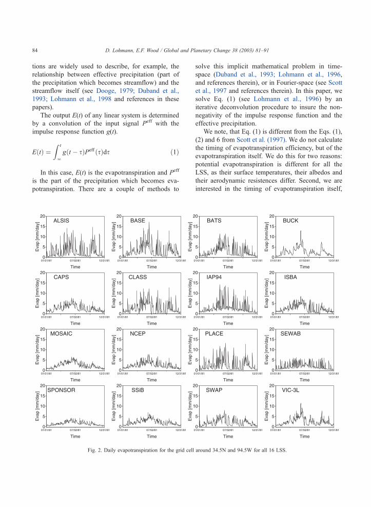
Liang et al. (1998) and Lohmann et al. (1998). Fig. 2

shows the modeled daily evapotranspiration for all

LSS in the year 1981 in the grid cell centered around

34.5N and 94.5W. Two differences are most impor-

tant. First, the models show maximum peak values of

evapotranspiration between 17 mm/day (BASE) and

4.5 mm/day (SPONSOR). Second, in the time period

in July without precipitation, some models have only

very little evapotranspiration (CLASS, PLACE) while

others still have significant contributions (CAPS,

IAP94, MOSAIC, NCEP, SEWAB, SPONSOR, see

also Fig. 13 in Lohmann et al., 1998). These two

results show that the LSS have differences in their

daily and monthly evapotranspiration response.

2. Analysis of timescales

The methods followed in this paper have been

outlined by Scott et al. (1997). However, their

approach was modified. We require non-negativity

D. Lohmann, E.F. Wood / Global and Planetary Change 38 (2003) 81–9182

in the calculation of the kernel function and fitted a

two-parameter model to the kernel function.

2.1. Convolution representation

The timescales of evapotranspiration response to a

precipitation event in a general circulation model

(GCM) have been described by Scott et al. (1997).

Although this relationship between precipitation and

evapotranspiration is known to be nonlinear, a simple

timescale analysis with kernel functions can provide

insight into the basic mechanisms and timing that

characterize the system.

A linear system can be characterized by its

impulse response function g(t), which in turn includes

all the necessary information about the response

timescales of the system. The theory of linear sys-

tems is well developed and impulse response func-

Fig. 1. Precipitation, potential evapotranspiration and the quotient for the months May–September, 1980–1986.

D. Lohmann, E.F. Wood / Global and Planetary Change 38 (2003) 81–91 83

tions are widely used to describe, for example, the

relationship between effective precipitation (part of

the precipitation which becomes streamflow) and the

streamflow itself (see Dooge, 1979; Duband et al.,

1993; Lohmann et al., 1998 and references in these

papers).

The output E(t) of any linear system is determined

by a convolution of the input signal Peff with the

impulse response function g(t).

EðtÞ ¼Z t

lgðt � sÞPeff ðsÞds ð1Þ

In this case, E(t) is the evapotranspiration and Peff

is the part of the precipitation which becomes eva-

potranspiration. There are a couple of methods to

solve this implicit mathematical problem in time-

space (Duband et al., 1993; Lohmann et al., 1996,

and references therein), or in Fourier-space (see Scott

et al., 1997 and references therein). In this paper, we

solve Eq. (1) (see Lohmann et al., 1996) by an

iterative deconvolution procedure to insure the non-

negativity of the impulse response function and the

effective precipitation.

We note, that Eq. (1) is different from the Eqs. (1),

(2) and 6 from Scott et al. (1997). We do not calculate

the timing of evapotranspiration efficiency, but of the

evapotranspiration itself. We do this for two reasons:

potential evapotranspiration is different for all the

LSS, as their surface temperatures, their albedos and

their aerodynamic resistences differ. Second, we are

interested in the timing of evapotranspiration itself,

Fig. 2. Daily evapotranspiration for the grid cell around 34.5N and 94.5W for all 16 LSS.


rather than evapotranspiration efficiency, as it is a

direct measure of the soil moisture timescale. Also

potential evapotranspiration was very inconsistent

among the models in the PILPS phase 2(c), varying

by an order of magnitude.

2.2. Fitting of the impulse response function

We used a simple two-parameter function to char-

acterize the impulse response function. Scott et al.

(1997) used a one-parameter decaying exponential

which is equivalent with the Antecedent Precipitation

Index (WMO, 1983). They suggested that due to a

multiplicity of timescales represented by the LSS, as

represented by different processes such as canopy

evaporation and transpiration, the appropriate func-

tional form would be a weighted combination of

several exponentials. We followed this approach, but

simplified it by fitting a weighted sum of a delta

function, d(t) and an exponential, exp� k t:

gðtÞ ¼ b*dðtÞ þ kexp�kt

b þ 1ð2Þ

where g(t) is the fitted impulse response function, b is

the weight for the delta function d, and 1/k is the e-

folding time. The reason for this functional form is

that it did fit the calculated impulse response function

well, because it reflects the typical model timescales

of a fast canopy evaporation response and slower

transpiration response. A one-parameter exponential

was not able to reproduce the basic shape of most

impulse response functions.

Fig. 3. Calculated and fitted impulse response function for the grid cell around 34.5N and 94.5W for all 16 LSS.


3. Analysis of PILPS Phase 2(c) results

The evapotranspiration timescales from the 16 LSS

of the PILPS Phase 2(c) were analysed as follows. We

first calculated the impulse response function for the

months of May–September for a 7-year period from

1980 to 1986 for all 61 grid cells and all LSS. The

seven impulse response functions for the different

years were then averaged and afterwards fitted with

Eq. (2).

Fig. 3 shows the averaged impulse response func-

tion for the same grid cell (centered around 34.5jNand 94.5jW) as in Fig. 2. The impulse response

functions show a large range in their values at time

0 as well as large differences in their timescale

T1/2 = ln(2)/k. A comparison with Fig. 2 shows that

those schemes whose evapotranspiration values have

the highest peaks (ALSIS, BASE, BATS, CLASS,

IAP94, PLACE) also have the highest values of the

impulse response function at time 0. The bucket model

(BUCK) is clearly different from all other models

because of the absence of a canopy interception

reservoir. It therefore does not represent very short

timescales of evapotranspiration, which is reflected by

small values of the impulse response function at time

0. The fact that the impulse response function of the

BUCK model has its peak value at the day after the

precipitation event can be explained by two reasons.

The net radiation and the vapor pressure deficit have

often larger values the day after the precipitation event.

Also, the daily precipitation was given uniformly over

24 h from 5:00 am or 6:00 am in the morning to the

same time the next morning. The soil of the BUCK

model therefore was often more moist the day after the

Fig. 4. Spatial distribution of the parameter k [1/day].


precipitation event than at the day of the precipitation

itself. The LSS with the longest timescales (IAP94,

MOSAIC, NCEP, SEWAB and SPONSOR) clearly

show a longer evapotranspiration persistence in the

summer months, as reflected by a lower k. The three

LSS (MOSAIC, SSiB and VIC-3L) which include

parameterizations of fractional coverage of precipita-

tion have the lowest values of the impulse response

function beside BUCK at time 0. Their parameter-

izations lead basically to a smaller canopy interception

storage for the whole grid cell and therefore less water

to directly re-evaporate.

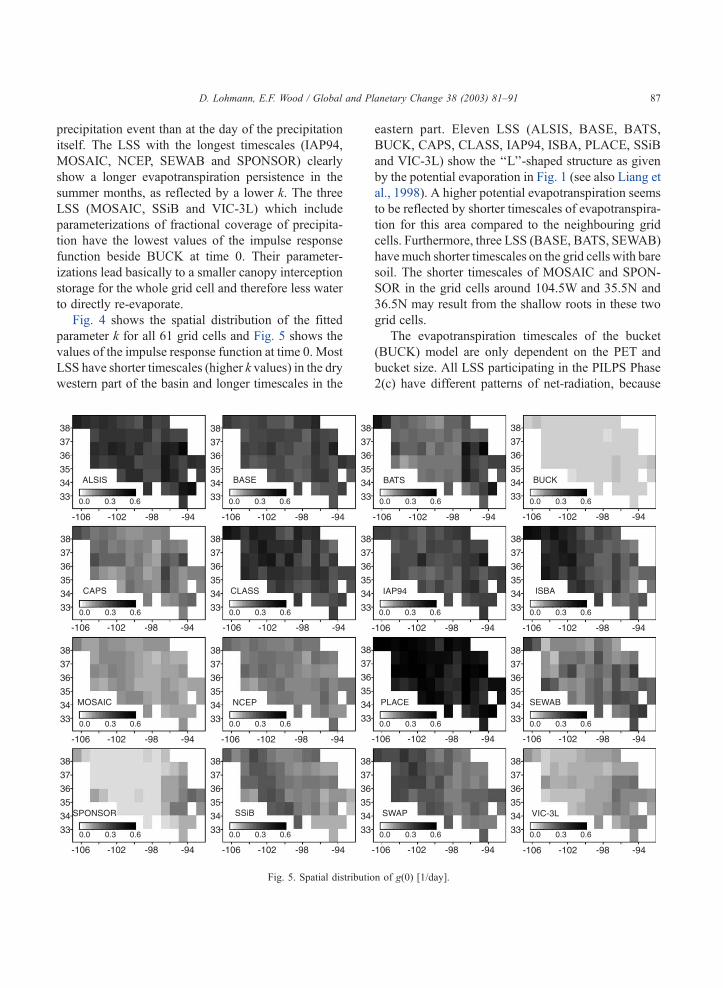
Fig. 4 shows the spatial distribution of the fitted

parameter k for all 61 grid cells and Fig. 5 shows the

values of the impulse response function at time 0. Most

LSS have shorter timescales (higher k values) in the dry

western part of the basin and longer timescales in the

eastern part. Eleven LSS (ALSIS, BASE, BATS,

BUCK, CAPS, CLASS, IAP94, ISBA, PLACE, SSiB

and VIC-3L) show the ‘‘L’’-shaped structure as given

by the potential evaporation in Fig. 1 (see also Liang et

al., 1998). A higher potential evapotranspiration seems

to be reflected by shorter timescales of evapotranspira-

tion for this area compared to the neighbouring grid

cells. Furthermore, three LSS (BASE, BATS, SEWAB)

havemuch shorter timescales on the grid cells with bare

soil. The shorter timescales of MOSAIC and SPON-

SOR in the grid cells around 104.5W and 35.5N and

36.5N may result from the shallow roots in these two

grid cells.

The evapotranspiration timescales of the bucket

(BUCK) model are only dependent on the PET and

bucket size. All LSS participating in the PILPS Phase

2(c) have different patterns of net-radiation, because

Fig. 5. Spatial distribution of g(0) [1/day].


of differences in surface temperature and albedo

(Liang et al., 1998). They therefore have different

patterns of PET. BUCK, for example, has a much

higher surface temperature than any other model,

which in turn shortens the evapotranspiration time-

scales. From Fig. 1, we can estimate the e-folding

times (see Delworth and Manabe, 1988) of the BUCK

to be on the order of 20–40 days; however, the

analysis from Fig. 4 shows that the calculated time-

scales are between 6 and 20 days, which basically

resulted from an overestimation of PET compared to

the Penman–Monteith estimation by a factor of 2.5

from BUCK. The reasons for this overestimation are

unclear, but could be related to the abnormal high

surface temperature (Liang et al., 1998). Note that the

Penman–Monteith equation itself is known to under-

estimate PET (Teillet and Holben, 1960). The regres-

sion of the inverse timescale 1/k with PET should be a

straight line for the BUCK model in the case of

constant bucket depth. The relationship of timescales

to PET can be seen in Fig. 6, which is a scatterplot of

PET against k for all 61 grid cells. The plot also shows

the regression line and the error of the slope. ALSIS,

CLASS, ISBA, MOSAIC, NCEP, SEWAB, and

SPONSOR show a small negative slope, indicating

that they have longer timescales in areas with higher

potential evapotranspiration. However, the error of the

slope is on the order of the slope itself.

All other models show the opposite behaviour,

especially BATS, BUCK and VIC-3L shorten their

evapotranspiration timescales with increasing PET.

The two grid cells around 35.5jN and 103.5jW and

104.5jW with bare soil were not taken into account

for the regression analysis, as some LSS have much

Fig. 6. Relationship between mean monthly potential evapotranspiration (May–September, 1980–1986) and k for 61 grid cells.


shorter timescales there. These two points are shown

as triangles in the figures.

Fig. 7 shows a scatterplot of the mean monthly

precipitation (from May to September) compared with

k. The LSS results can be categorized in three groups.

Ten LSS (ALSIS, BASE, CAPS, CLASS, IAP94,

ISBA, MOSAIC, NCEP, SEWAB, SSiB) have a

negative slope, which means that their evapotranspi-

ration timescales are longer in the humid eastern part

of the basin. Five LSS (BATS, BUCK, PLACE,

SPONSOR, SWAP) have a slope of the regression

close to zero, with one standard deviation of the slope

as large as the slope itself. One LSS (VIC-3L) has

longer evapotranspiration timescales in the dry west-

ern part of the basin. The result for the BUCK model

is not surprising, as its evapotranspiration timescale is

not a function of precipitation. However, it is interest-

ing to observe, that most LSS have longer timescales

in humid regions and shorter timescales in the dry

region. These models therefore show a fundamentally

different behaviour in their spatial distribution of

evapotranspiration timescales than the bucket model.

It cannot be concluded whether one model shows a

more realistic spatial pattern than the other models.

The final analysis has to be done with measurements.

4. Summary

This paper discusses the evapotranspiration time-

scales of 16 different land surface schemes which

participated in the Project for Intercomparison of

Land-surface Parameterization Schemes (PILPS)

Phase 2(c) Red-Arkansas River experiment. Although

Fig. 7. Relationship between mean monthly precipitation (May–September, 1980–1986) and k for 61 grid cells.


a simple analysis with a linear system can only approx-

imate the modeled timescales, we think that such an

analysis is a valuable tool for the comparison of LSS.

LSS are normally described with parameterizations ‘‘as

physical as possible’’ (with which they refer to detailed

descriptions of local scale bio-physical parameteriza-

tions) but do neglect the typical timescales of in-

teraction implicit to these parameterizations and

interactions with other parts of the LSS (e.g. vertical

transports of water with Richards equation, Hillel,

1982).

The 16 LSS have very different timescales across

the Red-Arkansas River basin. LSS have a tendency

to become more and more complicated over time.

Although many of the parameterizations seem to be

necessary to have a realistic description of the land

surface, we think that it is time to take a look at the

typical timescales inherent in the complex nonlinear

interactions.

The analysis in this paper showed that the LSS,

which participated in the PILPS Phase 2(c), have

differences in their timeseries of modeled evapotrans-

piration, up to a factor of 4 in their peak values after

precipitation events. The timing of evapotranspiration

was described by a two-parameter impulse response

(kernel) function. This kernel function resolves two

different timescales which are included in most param-

eterizations of land surface processes. We believe that

there are typical impulse response functions for differ-

ent climates and think that the knowledge of such a

function could yield to more simple descriptions of the

complex interactions within LSS. This is especially

important.

We did not have long-term evapotranspirationmeas-

urements in the basin, and therefore we cannot con-

clude which one of the LSS response timescales is more

realistic. Such a comparison might be interesting and

was already requested by Koster and Suarez (1996) and

Scott et al. (1995). The atmospheric budget as used by

Liang et al. (1998) and Lohmann et al. (1998) was too

noisy on a daily timescale to allow for the estimation of

an impulse response function for the whole basin.

Acknowledgements

The PILPS Phase 2(c) participants are gratefully

acknowledged: Aaron Boone, Sam Chang, Fei Chen,

Yongjiu Dai, Carl Desborough, Robert E. Dickinson,

Qingyun Duan, Michael Ek, Yeugeniy M. Gusev,

Florence Habets, Parviz Irannejad, Randy Koster,

Dennis P. Lettenmaier, Xu Liang, Kenneth E.

Mitchell, Olga N. Nasonova, Joel Noilhan, John

Schaake, Adam Schlosser, Yaping Shao, Andrey B.

Shmakin, Diana Verseghy, Kirsten Warrach, Peter

Wetzel, Yongkang Xue, Zong-Liang Yang and Qing-

cun Zeng.

References

Delworth, T., Manabe, S., 1988. The influence of potential evapo-

ration on the variabilities of simulated soil wetness and climate.

J. Clim. 1, 523–547.

Dooge, J., 1979. Deterministic input–output models. In: Lloyd, E.,

O’Donell, T., Wilkinson, J. (Eds.), The Mathematics of Hydrol-

ogy and Water Resources. Academic Press, London, pp. 1–37.

Duband, D., Obled, C., Rodriguez, J., 1993. Unit hydrograph re-

visited: an alternate iterative approach to UH and effective pre-

cipitation identification. J. Hydrol. 150, 115–149.

Hillel, D., 1982. Introduction to Soil Physics. Academic Press,

San Diego.

Koster, R., Suarez, M., 1996. The influence of land surface mois-

ture retention on precipitation statistics. J. Clim. 9, 2551–2567.

Liang, X., Wood, E., Lettenmaier, D., Lohmann, D., Boone, A.,

Chang, S., Chen, F., Dai, Y., Desborough, C., Dickinson, R.,

Duan, Q., Ek, M., Gusev, Y., Habets, F., Irannejad, P., Kos-

ter, R., Mitchell, K., Nasonova, O., Noilhan, J., Schaake, J.,

Schlosser, A., Shao, Y., Shmakin, A., Verseghy, D., Wang, J.,

Warrach, K., Wetzel, P., Xue, Y., Yang, Z., Zeng, Q., 1998.

The Project for Intercomparison of Land-surface Parameter-

ization Schemes (PILPS) Phase 2(c) Red-Arkansas River ba-

sin experiment: 2. Spatial and temporal analysis of energy

fluxes. Global Planet. Change 19, 137–159.

Lohmann, D., Nolte-Holube, R., Raschke, E., 1996. A large scale

horizontal routing model to be coupled to land surface param-

eterization schemes. Tellus 48 A, 708–721.

Lohmann, D., Lettenmaier, D., Liang, X., Wood, E., Boone, A.,

Chang, S., Chen, F., Dai, Y., Desborough, C., Dickinson, R.,

Duan, Q., Ek, M., Gusev, Y., Habets, F., Irannejad, P., Kos-

ter, R., Mitchell, K., Nasonova, O., Noilhan, J., Schaake, J.,

Schlosser, A., Shao, Y., Shmakin, A., Verseghy, D., Wang, J.,

Warrach, K., Wetzel, P., Xue, Y., Yang, Z., Zeng, Q., 1998.

The Project for Intercomparison of Land-surface Parameter-

ization Schemes (PILPS) Phase 2(c) Red-Arkansas River ba-

sin experiment: 3. Spatial and temporal analysis of water

fluxes. Global Planet. Change 19, 161–179.

Scott, R., Koster, R., Entekhabi, D., Suarez, M., 1995. Effect of a

canopy interception reservoir on hydrological persistence in a

general circulation model. J. Clim. 8, 1917–1922.

Scott, R., Entekhabi, D., Koster, R., Suarez, M., 1997. Timescales of

land surface evapotranspiration response. J. Clim. 10, 559–566.

Shuttleworth, W., 1993. Evaporation. In: Maidment, D.R. (Ed.),


Handbook of Hydrology. McGraw Hill, New York, pp. 4.1–

4.53. Chap. 4.

Teillet, P., Holben, B., 1960. Potential evapotranspiration estimates

by the approximate energy balance method of Penman. J. Geo-

phys. Res. 65, 3391–3413.

WMO, 1983. Guide to Hydrologic Practices, number 168. World

Meteorological Organization Publ., Geneva.

Wood, E., Lettenmaier, D., Liang, X., Lohmann, D., Boone, A.,

Chang, S., Chen, F., Dai, Y., Dickinson, R., Duan, Q., Ek, M.,

Gusev, Y., Habets, F., Irannejad, P., Koster, R., Mitchell, K.,

Nasonova, O., Noilhan, J., Schaake, J., Schlosser, A., Shao, Y.,

Shmakin, A., Verseghy, D., Wang, J., Warrach, K., Wetzel, P.,

Xue, Y., Yang, Z., Zeng, Q., 1998. The Project for Intercom-

parison of Land-surface Parameterization Schemes (PILPS)

Phase 2(c) Red-Arkansas River experiment: 1. Experiment de-

scription and summary intercomparisons. Global Planet.

Change 19, 115–135.


timescales of land surface evapotranspiration response in

Documents