Time Synchronization Services for Wireless Sensor Networks

Dissertation Proposal

Jeremy ElsonDepartment of Computer Science

University of California, Los AngelesLos Angeles, CA, 90095

jelson@cs.ucla.edu

April 10, 2001

Abstract

Time synchronization is a critical piece of infrastructure for any distributed system. Distributed,wireless sensor networks make extensive use of synchronized time in many contexts—for example, informing TDMA schedules, integrating a time-series of proximity detections into a velocity estimate, indetecting redundant detections of a phenomenon from multiple sensors, and in distributed beamformingsystems. The variety of uses leads to highly varied and non-standard requirements in the scope, lifetime,and maximum error of the synchronization achieved, as well as the time and energy required to achieveit. Existing time synchronization methods were not created with wireless sensor networks in mind, andneed to be extended or redesigned to meet the new requirements and constraints.

Our proposed work centers around the development of new time synchronization methods, theircharacterization according to metrics relevant to wireless sensor networks, and a proof-of-concept im-plementation of an application that makes use of our synchronization primitives. In this proposal, we firstdescribe a number of metrics that we have found useful for the characterization of time synchronizationservices. Using these metrics, we describe existing services, and compare them to the synchroniza-tion requirements of future sensor networks. We also present an implementation of our own low-powersynchronization scheme, post-facto synchronization, and describe an experiment that characterizes itsperformance for creating short-lived and localized but high-precision synchronization using very littleenergy. Finally, we describe our work plan.

Contents

1. Introduction 11.1. Wireless Sensor Networks . . . . . . . . . . . . . . . . . . . . . . . . . . . . . . . . . . . 11.2. Time Synchronization . . . . . . . . . . . . . . . . . . . . . . . . . . . . . . . . . . . . . 1

2. Metrics and Terminology 2

3. Motivations 33.1. Distributed beam-forming and sensor fusion . . . . . . . . . . . . . . . . . . . . . . . . . 33.2. Multi-sensor integration . . . . . . . . . . . . . . . . . . . . . . . . . . . . . . . . . . . . 43.3. In network data aggregation and duplicate suppression . . . . . . . . . . . . . . . . . . . . 53.4. Energy-efficient radio scheduling . . . . . . . . . . . . . . . . . . . . . . . . . . . . . . . 53.5. Uses common in traditional distributed systems . . . . . . . . . . . . . . . . . . . . . . . . 6

4. Related Work 64.1. Distributed Clocks and Network Time Protocols . . . . . . . . . . . . . . . . . . . . . . . 64.2. National Time Standards and Time Transfer . . . . . . . . . . . . . . . . . . . . . . . . . . 74.3. Methods for avoiding the problem . . . . . . . . . . . . . . . . . . . . . . . . . . . . . . . 8

5. Sensor Network Time 95.1. The Need for Something New . . . . . . . . . . . . . . . . . . . . . . . . . . . . . . . . . 95.2. Design Principles . . . . . . . . . . . . . . . . . . . . . . . . . . . . . . . . . . . . . . . . 10

5.2.1 . Multi-modal synchronization . . . . . . . . . . . . . . . . . . . . . . . . . . . . . 105.2.2 . Tiered architectures . . . . . . . . . . . . . . . . . . . . . . . . . . . . . . . . . . 10

5.3. Our Approach . . . . . . . . . . . . . . . . . . . . . . . . . . . . . . . . . . . . . . . . . 11

6. Post-Facto Synchronization 116.1. Expected Sources of Error . . . . . . . . . . . . . . . . . . . . . . . . . . . . . . . . . . . 126.2. Empirical Study . . . . . . . . . . . . . . . . . . . . . . . . . . . . . . . . . . . . . . . . 136.3. Discussion . . . . . . . . . . . . . . . . . . . . . . . . . . . . . . . . . . . . . . . . . . . 14

7. Work Plan 157.1. Development and characterization of time sync methods . . . . . . . . . . . . . . . . . . . 157.2. Testbed implementation as proof-of-concept . . . . . . . . . . . . . . . . . . . . . . . . . 167.3. Exploration of methods for tuning and automatic modality selection . . . . . . . . . . . . . 17

8. Conclusions 18

Bibliography 18

i

1. Introduction

1.1. Wireless Sensor Networks

Recent advances in miniaturization and low-cost, low-power design have led to active research in large-scale, highly distributed systems of small, wireless, low-power, unattended sensors and actuators [ADL

�

98,KKP99, EGHK99]. The vision of many researchers is to create sensor-rich “smart environments” throughplanned or ad-hoc deployment of thousands of sensors, each with a short-range wireless communicationschannel, and capable of detecting ambient conditions such as temperature, movement, sound, light, or thepresence of certain objects.

While this new class of distributed systems has the potential to enable a wide range of applications,it also poses serious design challenges, described more fully by KKP [KKP99] and EGHK [EGHK99].The sheer number of these devices makes global broadcasting undesirable; wireless nodes’ limited com-munication range relative to the geographic area spanned by the system often makes global broadcastingso inefficient that it is infeasible. As a consequence, many argue that nodes must depend on localizedalgorithms—making control decisions based solely on interactions with neighbors, without global systemknowledge [EGHK99, IGE00].

Another important feature that distinguishes sensor networks from traditional distributed systems is theirneed for energy efficiency. Many nodes in the emerging sensor systems will be untethered, having only finiteenergy reserves from a battery. Unlike laptops or other handheld devices that enjoy constant attention andmaintenance by humans, the scale of a sensor net’s deployment will make replenishment of these reservesimpossible. This requirement pervades all aspects of the system’s design. For example, nodes must remainoff or in a low-power state as often as possible; when on, they must maximize the usefulness of every bittransmitted or received [PK00].

1.2. Time Synchronization

Time synchronization is a critical piece of infrastructure for any distributed system. Distributed, wirelesssensor networks make particularly extensive use of synchronized time: for example, to integrate a time-series of proximity detections into a velocity estimate [CEE

�

01]; to measure the time-of-flight of sound forlocalizing its source [Gir00]; to distribute a beamforming array [YHR

�

98]; or to suppress redundant mes-sages by recognizing that they describe duplicate detections of the same event by different sensors [IGE00].Sensor networks also have many of the same requirements as traditional distributed systems: accurate times-tamps are often needed in cryptographic schemes, to coordinate events scheduled in the future, for orderinglogged events during system debugging, and so forth.

The broad nature of sensor network applications leads to timing requirements whose scope, lifetime, andmaximum error differ from traditional systems. In addition, many nodes in the emerging sensor systemswill be untethered and therefore have small energy reserves. All communication—even passive listening—will have a significant effect on those reserves. Time synchronization methods for sensor networks musttherefore also be mindful of the time and energy that they consume.

In this paper, we argue that the heterogeneity of requirements across sensor network applications, theneed for energy-efficiency and other constraints not found in conventional distributed systems, and eventhe variety of hardware on which sensor networks will be deployed, make current synchronization schemesinadequate to the task. In sensor networks, existing time synchronization methods will need to beextended and combined in new ways in order to provide service that meets the needs of applicationswith the minimum possible energy expenditures. The development of these new methods is the core ofour proposal.

1

We will also present our idea for post-facto synchronization, an extremely low-power method of syn-chronizing clocks in a local area when accurate timestamps are needed for specific events. We also presentan experiment that suggests this multi-modal scheme is capable of achieving a maximum error on the orderof

���sec—an order of magnitude better than either of the two modes of which it is composed. These re-

sults are encouraging, although still preliminary and performed under idealized laboratory conditions. Webelieve that our pilot study lends weight to our methods and that further investigation is warranted.

We begin our discussion in Section 2, describing a number of metrics that can be used to classify boththe types of service provided by synchronization methods and the requirements of applications that usethose methods. In Section 3, we justify in more detail the need for synchronized time in sensor networks.Related work is reviewed in Section 4. Section 5 argues why the existing work in the field is insufficientfor use in the new sensor network regime, and outlines our proposed contributions. Section 6 describes ourpost-facto synchronization technique and presents an experiment that characterizes its performance. Ourproposed thesis work plan is described in detail in Section 7, and conclusions are drawn in Section 8.

2. Metrics and Terminology

Before starting our discussion in earnest, we will first define a set of metrics that we have found usefulfor characterizing time synchronization in sensor networks. In studying both methods and applications, wehave found five metrics to be especially important:

� Maximum Error—either the dispersion among a group of peers, or maximum deviation of the mem-bers from an external standard.

� Lifetime—which can range from persistent synchronization that lasts as long as the network operates,to nearly instantaneous (useful, for example, if nodes want to compare the detection time of a singleevent).

� Scope and Availability—the geographic span of nodes that are synchronized, and completeness ofcoverage within that region.

� Efficiency—the time and energy expenditures needed to achieve synchronization.

� Cost and Form Factor—which can become particularly important in wireless sensor networks thatinvolve thousands of tiny, disposable sensor nodes.

The services provided by different time synchronization methods fall into many disparate points in thisparameter space. All of them make tradeoffs—no single method is optimal along all axes.

To illustrate the use of these metrics, consider the time service provided by the U.S. Global PositioningSystem [Kap96] (described in more detail in Section 4). Consumer GPS receivers can synchronize nodesto a persistent-lifetime time standard that is Earth-wide in scope within a maximum of 200ns [MKMT99].However, GPS units often can not be used (e.g., inside structures, underwater, during Mars exploration),can require several minutes of settling time. In some cases, GPS units might also be large, high-power andexpensive compared to small sensors.

In contrast, consider a small group of nodes with short-range, low-power radios. If one node transmitsa signal, the others can use that signal as a time reference—for example, to compare the times at whichthey recorded a sound. The synchronization provided by this simple “pulse” is local in scope and its error

2

comes primarily from variable delays on the radio receivers and propagation delay of the radio waves. Fora given error bound, the lifetime of the synchronization is also finite as the nodes’ clocks will wander afterthe initial pulse. However, the pulse is fast and energy-efficient because it only requires the transmission ofa single signal.

3. Motivations

Why do sensor nets need synchronized time?Before discussing time synchronization methods, we must first clarify its motivations. In this section,

we will describe some common uses of synchronized time in sensor networks. The wide net cast by thedisparate application requirements is important; we will argue later that it precludes the use of any singlesync method for all applications. Indeed, while the related work in this field (reviewed in Section 4) isextensive, it often relies on assumptions that are violated in the new sensor network regime.

3.1. Distributed beam-forming and sensor fusion

In recent years, interest has grown in signal processing techniques such as sensor fusion and beam-forming.These are techniques used to combine the inputs of multiple sensors, sometimes using heterogeneous modal-ities, in applications such as noise reduction [YHR

�

98], target tracking, and process control. This kind ofDSP will serve as an important basis for sensor networks, but much of the extensive prior art in the fieldassumes centralized sensor fusion. That is, even if the sensors gathering data are distributed, sensor datais often assumed to be consolidated at one site before processing. However, centralized processing makesuse of implicit time synchronization; synchronization that must be made explicit to create a fully distributedsystem.

For example, consider a beamforming array designed to localize the source of sound, such as thatdescribed by YHRCL in [YHR

�

98]. The array computes phase differences of signals received by sensorsat different locations. From these phase differences, the processor can infer the time of flight of the soundfrom its source to each sensor. This allows the sound’s source to be localized with respect to the spatialreference frame defined by the sensors in the array. However, this makes the implicit assumption thatthe sensors themselves are synchronized in time, as well. In other words, the beam-forming computationassumes that the observed phase differences are due to differences in the time of flight from the sound sourceto the sensor, and not variable delays incurred in transmitting signals from the sensor to the processor. Ina centralized system, where there is tight coupling from sensors to a single central processor, this is a validassumption; the sensor data share an implicitly synchronized time-base by virtue of the fact that the audiodata are all fed to the same processor. However, for such an array to be implemented on a fully distributedset of autonomous wireless sensors, explicit time synchronization of the sensors is needed.

It is important to note that a beam-forming array actually contains two separate (but related) time-synchronization problems. Specifically, to measure the time-of-flight from the sound’s source to the receiv-ing sensors, some form of synchronization must exist between the sender and receiver. In other words, thearray needs to know the time of emission relative to the time of detection in order to measure time-of-flight.This latter problem has traditionally been solved with “over-sampling”: treating the clock bias between theemitter and receivers as an extra unknown in the system of localization equations, and adding an extra sen-sor measurement to balance the extra unknown. This works only if the receivers are synchronized with eachother; that is, if there is only a single clock bias between the sender and any receiver. Therefore, the needfor explicit receiver synchronization as described earlier is not obviated by having extra sensors. Without

3

correlated receivers, each additional sensor brings with it both a measurement and its own unknown clockbias—i.e., adding both an equation and an unknown to the system.

3.2. Multi-sensor integration

A common theme in sensor network design is that of multi-sensor integration—combining informationgleaned from multiple sensors into a larger world-view not detectable by any single sensor alone. Unlikethe previous examples, in which sensor fusion is done at the signal processing level, sensor integrationfocuses on algorithmically combining higher-level knowledge.

For example, consider a group of nodes that know their geographic positions and can each detect prox-imity to some static phenomenon

�. (The detection might involve localization as described in the previous

section.) Alone, a single sensor can tell that it is near�

. However, by integrating their knowledge, the jointnetwork can describe more than just a set of locations covered by

�; it can also compute

�’s size. In some

sense, the whole of information has become greater than the sum of the parts.This type of emergent behavior does not always require synchronized time. If

�is static, as in the

previous example, time sync may not be needed at all. However, what if�

is moving, and the objective isto report

�’s speed and direction? At first glance, it might seem that the object localization system we de-

scribed above can be easily converted into a motion tracking system, simply by performing repeated queriesof the object tracking system over time. If the data indicating the location of our tracked phenomenon

�

all arrives at the same processor for integration, perhaps no synchronization across nodes is required. Theintegrator can simply timestamp each localization reading as it arrives and will then have all the informationrequired to integrate the series into motion data. In this case, it seems that the time synchronization problemhas been avoided entirely.

This scheme has serious limitations discussed below, but it does work in some contexts. In particular, ifthe tracked object is moving very slowly relative to the delay between the sensors and the integration point,our brute force approach might work. For example, imagine an asset tracking system capable of locatingspecific pieces of equipment. If we wish to define the “motion” of an object as the history of all people whohave used it, an equipment motion tracker might be designed very simply. We can merely ask the objecttracker for the equipment’s location several times a day, and compile a list over time of offices in which theequipment has been located. This works because we assume someone who uses equipment does so over thecourse of days or weeks – extremely slowly on the timescale over which the object-tracker can locate anobject and report its location to the user or a data integrator.

This method has serious limitations in contexts where the timing requirements are more critical than inour equipment example. If the tracked phenomenon moves quickly, many factors that were insignificantin equipment tracking become overwhelming. For example, consider the situation likely in wireless sensornetworks: a spatially distributed group of sensors, each capable of communication over a very short rangecommunication relative to the total geographic area of sensor coverage. Information can only travel throughthis network hop-by-hop; therefore, the latency of messages from any given sensor to a central integratorwill vary with the distance from the sensor to the integration point. In this situation, the brute force approachmay fail.

The reason for the failure of the brute force approach is instructive to consider. The simple equipmenttracker essentially assumed that the travel time of messages from the equipment sensors back to the inte-gration point was zero: we ask the question “Where is this object?” and receive a reply that we assumeis instantaneous and still correct when it is received. In the case of tracking equipment, this is probably avalid assumption because a specific piece of equipment is unlikely to move on the scale of time required to

4

propagate a message through the sensor network. However, this assumption breaks down for faster-movingphenomena. Using the brute force centralized approach, it will be impossible to accurately track the motionof any phenomenon moving at speeds that approach the time scale of the networks’ round trip time.

There are additional motivations for doing localized and distributed detection. A centralized aggregationpoint is not scalable and is prone to failures. In addition, in sensor networks where energy-efficiency iscritical, it is unwise to design a system where a large volume of messages must be routed through manypower-consuming nodes. A system that transmits each individual location reading through every node onthe path from the phenomenon back to the integration point will have a high energy cost.

These limitations suggest that sensor readings should be time-stamped inside of the network, as nearas possible to the original sensor event. Doing so dramatically reduces the variable delay introduced bymessage transmission latencies. Timestamping inside the network also allows tracking data to be post-processed into motion data, aggregated, and summarized inside of the network, thus requiring a greatlyreduced number of bits to travel back to the user. All of these advantages, however, do come with a price:sensors in the network must share a common time base in order to ensure the consistency of readings takenat multiple sensors.

In a motion tracking application, the allowable synchronization error in nodes’ clocks is informed byfactors such as the speed of the target relative to sensor density and detection range. It is also affected by thesystem’s desired spatial precision and detection frequency. The tighter time synchronization is achieved,the greater precision is possible in the tracking of motion by a collection of proximity detectors. Veryslow moving objects may be tracked sufficiently by nodes with loosely synchronized clocks, but tighter andtighter synchronization is required if we wish to track faster and faster objects—or perhaps even phenomenasuch as wave-fronts.

3.3. In network data aggregation and duplicate suppression

A feature common to sensor networks due to the high energy cost of communication compared to com-putation [PK00] is local processing, summarization, and aggregation of data in order to minimize the sizeand frequency of transmissions. Suppression of duplicate notifications of the same event from a group ofnearby sensors can result in significant energy savings [IGE00]. To recognize duplicates, events must betimestamped with a precision on the same order as the event frequency; this might only be tens or hundredsof milliseconds. Since the data may be sent a long way through the network and even cached by manyof the intermediate nodes, the synchronization must be broad in scope and long in lifetime—perhaps evenpersistent.

3.4. Energy-efficient radio scheduling

Low-power, short-range radios of the variety typically used for wireless sensor networks expend virtuallyas much energy passively listening to the channel as they do during transmission [PK00, APK00]. Sensornet MAC protocols are frequently designed around this assumption, aiming to keep the radio off for as longas possible. TDMA is a common starting point because of the natural mechanism it provides for adjustingthe radio’s duty cycle, trading energy expenditure for other factors such as channel utilization and messagelatency [Soh00].

While distributed time synchronization is central to any TDMA scheme, it is considerably more impor-tant in wireless sensor nets than in traditional (e.g. cellular phone) TDMA networks. Traditional wirelessMAC protocols value only high channel utilization. Good time sync is therefore important because it short-

5

ens the guard time, but also easy because each frame received implicitly imparts information about thesender’s clock. This information can be used to frequently re-synchronize a node’s clock with those of itspeers [LS96].

In sensor networks, the picture changes considerably. Energy-efficiency is the highest priority, so local-ized algorithms are used to minimize both the size and frequency of messages. Long inter-message intervalsresult in greater clock drift and therefore longer guard times. The high energy cost of passive listening de-scribed above makes these guard times expensive. In addition, small data payloads make the guard timesa large proportion of the total time a receiver is listening. These factors make good clock synchronizationcritical for saving energy, and suggest a new technique is needed to achieve it.

3.5. Uses common in traditional distributed systems

The uses of time synchronization we have described so far have been specific to sensor networks, relatingto their unique requirements in distributed signal processing, energy efficiency, and localized computation.However, at its core, a sensor network is also a distributed system, where time synchronization of vari-ous forms has been used extensively for some time. Many of these more traditional uses apply in sensornetworks as well. For example:

� Logging and Debugging. During design and debugging, it is often necessary correlate logs of manydifferent nodes’ activities to understand the global system’s behavior. Logs without synchronizedtime often make it difficult or impossible to determine causality, or reconstruct an exact sequence ofevents.

� Interaction with Users. People use “civilian time”—their wristwatches—when making requests suchas “show me activity in the southeast quadrant between midnight and 4 A.M.” For this request to bemeaningful, certain nodes in a sensor net need to be synchronized with an external time standard. Insome sense, this may be an orthogonal requirement to those discussed previously; many applicationsof time-sync only require internal consistency.

� Cryptography. Perhaps due to sensor nets’ applicability in military applications, there has alreadybeen significant interest in cryptographically protecting sensor network messages [HSW

�

, Hil]. Cer-tain authentication schemes, such as the Kerberos Authentication Service [SNS88], depend on syn-chronized time to prevent replay attacks and other forms of circumvention.1

� Database Consistency. Database update protocols often require synchronized time to serialize trans-actions or eliminate duplicate updates (for example, in [LSW91]). There has been recent interest inexpanding the domain of databases to encompass embedded sensor network queries [BGS01], usingdatabases running inside the network itself.

4. Related Work

4.1. Distributed Clocks and Network Time Protocols

Perhaps the seminal work in computer clock synchronization is Lamport’s work that elucidates the impor-tance of virtual clocks in systems where causality is more important than absolute time [Lam78]. In his

1Davis and Geer point out in [DGT96] that, in some contexts such as Kerberos, challenge-response can take the place of accuratetimestamps.

6

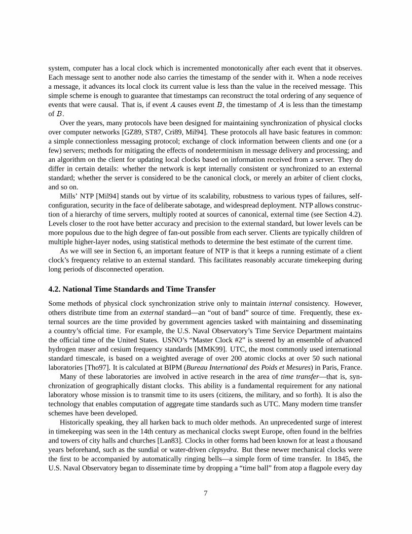
system, computer has a local clock which is incremented monotonically after each event that it observes.Each message sent to another node also carries the timestamp of the sender with it. When a node receivesa message, it advances its local clock its current value is less than the value in the received message. Thissimple scheme is enough to guarantee that timestamps can reconstruct the total ordering of any sequence ofevents that were causal. That is, if event

�causes event � , the timestamp of

�is less than the timestamp

of � .Over the years, many protocols have been designed for maintaining synchronization of physical clocks

over computer networks [GZ89, ST87, Cri89, Mil94]. These protocols all have basic features in common:a simple connectionless messaging protocol; exchange of clock information between clients and one (or afew) servers; methods for mitigating the effects of nondeterminism in message delivery and processing; andan algorithm on the client for updating local clocks based on information received from a server. They dodiffer in certain details: whether the network is kept internally consistent or synchronized to an externalstandard; whether the server is considered to be the canonical clock, or merely an arbiter of client clocks,and so on.

Mills’ NTP [Mil94] stands out by virtue of its scalability, robustness to various types of failures, self-configuration, security in the face of deliberate sabotage, and widespread deployment. NTP allows construc-tion of a hierarchy of time servers, multiply rooted at sources of canonical, external time (see Section 4.2).Levels closer to the root have better accuracy and precision to the external standard, but lower levels can bemore populous due to the high degree of fan-out possible from each server. Clients are typically children ofmultiple higher-layer nodes, using statistical methods to determine the best estimate of the current time.

As we will see in Section 6, an important feature of NTP is that it keeps a running estimate of a clientclock’s frequency relative to an external standard. This facilitates reasonably accurate timekeeping duringlong periods of disconnected operation.

4.2. National Time Standards and Time Transfer

Some methods of physical clock synchronization strive only to maintain internal consistency. However,others distribute time from an external standard—an “out of band” source of time. Frequently, these ex-ternal sources are the time provided by government agencies tasked with maintaining and disseminatinga country’s official time. For example, the U.S. Naval Observatory’s Time Service Department maintainsthe official time of the United States. USNO’s “Master Clock #2” is steered by an ensemble of advancedhydrogen maser and cesium frequency standards [MMK99]. UTC, the most commonly used internationalstandard timescale, is based on a weighted average of over 200 atomic clocks at over 50 such nationallaboratories [Tho97]. It is calculated at BIPM (Bureau International des Poids et Mesures) in Paris, France.

Many of these laboratories are involved in active research in the area of time transfer—that is, syn-chronization of geographically distant clocks. This ability is a fundamental requirement for any nationallaboratory whose mission is to transmit time to its users (citizens, the military, and so forth). It is also thetechnology that enables computation of aggregate time standards such as UTC. Many modern time transferschemes have been developed.

Historically speaking, they all harken back to much older methods. An unprecedented surge of interestin timekeeping was seen in the 14th century as mechanical clocks swept Europe, often found in the belfriesand towers of city halls and churches [Lan83]. Clocks in other forms had been known for at least a thousandyears beforehand, such as the sundial or water-driven clepsydra. But these newer mechanical clocks werethe first to be accompanied by automatically ringing bells—a simple form of time transfer. In 1845, theU.S. Naval Observatory began to disseminate time by dropping a “time ball” from atop a flagpole every day

7

precisely at noon [BD82]. The ball was often used by ships anchored in the Potomac river that needed acalibrated chronometer for navigation before setting out to sea [SA98].

In modern times, the state of the art is in radio time transfer methods. The first of these, seen originally inthe 1920’s, was the a voice announcer on radio station WWV operated by the National Institute of Standardsand Technology. WWV is still in operation today, along with its more recent cousin, WWVB, whichprovides computer-readable signals in stead of voice announcements. The modern-day service providesreferences to U.S. time and frequency standards within one part in

�������.

The most active subject of modern-day research is in two-way satellite time transfer [SPK00]. TWSTTallows two clocks connected by a satellite relay to both compute their offset from their peer. It is superiorto methods such as WWV’s radio broadcasts because it transfer is two-way, instead of solely from sender toreceiver. Use of satellites also allows intercontinental time transfer. TWSTT methods are used to connectthe time and frequency standards of national laboratories to BIPM in France for computation of internationaltimescales.

Satellite navigation systems—most notably, GPS [Kap96]—have an important relationship to time. GPSprovides localization service by allowing users to measure time of flight of radio signals from satellites (atknown locations) to a receiver. The system needs synchronized time for the scheme to work; it also providesone-way time transfer to the user as a “side effect” of localization. (Recent work has focused on using GPSfor two-way time transfer as well [LL99].) Although a complete discussion of the technical details is beyondthe scope of this document, it is important to note that GPS is both a user and disseminator of USNO’stimescale. Consumer GPS receivers can synchronize nodes to UTC(USNO) within 200ns [MKMT99].

4.3. Methods for avoiding the problem

In some cases, the time synchronization problem can be solved by not solving it—designing the system toavoid the need for the problem to be solved. A number of systems exemplify this design principle. Specifi-cally, it is instructive to reconsider several localization and ranging systems. (The relationship between timeand space is closely intertwined; time synchronization often goes hand in hand with localization.)

Many localization systems estimate the distance between two points by measuring the time-of-flight ofsome phenomenon from one point to the other. Generally speaking, a system emits a recognizable signalat a sender � , then times the interval required for the signal to arrive at a receiver � . If the propagationspeed of the phenomenon is known, the time measurement can be converted to distance. The fundamentalproblem that must be solved is synchronizing � and � in time so that the propagation delay can be properlymeasured. We will briefly examine three systems that solve this problem in three different ways.

Pinpoint, Inc.’s RF-ID system [?] avoids the synchronization problem by setting ��� ; that is, making� and � the same node. The RF-ID system emits an RF pulse which is modulated by the target and reflectedback to the sender. The sender and receiver are implicitly synchronized by virtue of being the same device.This allows a measurement of the signal’s round-trip time, and therefore the range from the sender/receiverto the target.

The GPS satellite system, mentioned earlier, also localizes by measuring the time-of-flight of RF signals.GPS also avoids synchronizing � (the satellites) with � (the user’s receiver) by treating the clock biasbetween � and � as an unknown. Because there are many redundant sending satellites, the receiver canlock onto one additional satellite, solving for its � ��������������� instead of only � ����������� . As we discussedearlier in Section 3.1, this only works by virtue of the senders being synchronized with each other.

Finally, ORL’s Active Bat system [WJH97] synchronizes � with � by using a synchronization modalitydifferent from the measurement modality. In their system, modulo certain details, � simultaneously emits

8

a (fast) RF pulse and a (slow) ultrasound pulse. The time of flight of the RF pulse is negligible comparedto that of the ultrasound. The RF pulse can be considered an instantaneous phenomenon that establishessynchronization between � and � with respect to the ultrasound pulse.

Of course, the localization application (and these implementations in particular) are only representative.Many other systems use similar designs to avoid the need for synchronized clocks. For example, in theLOCUS distributed operating system [PWB

�

87], consistency of distributed filesystem operations is ensuredby dynamically selecting a single node as a synchronization point for a particular file-descriptor. By forcingall file operations to go through the synchronization point, no clock sync is needed to achieve maintain aconsistent view of the total ordering of file events.

5. Sensor Network Time

5.1. The Need for Something New

We argued in Section 3 that it is important for sensor networks to have access to synchronized time. How-ever, in Section 4, we described a wide variety of methods for synchronizing time. Is something newneeded?

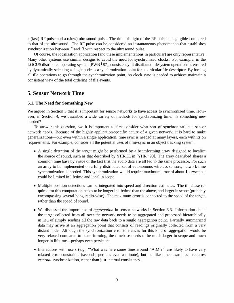
To answer this question, we it is important to first consider what sort of synchronization a sensornetwork needs. Because of the highly application-specific nature of a given network, it is hard to makegeneralizations—but even within a single application, time sync is needed at many layers, each with its onrequirements. For example, consider all the potential uses of time-sync in an object tracking system:

� A single detection of the target might be performed by a beamforming array designed to localizethe source of sound, such as that described by YHRCL in [YHR

�

98]. The array described shares acommon time base by virtue of the fact that the audio data are all fed to the same processor. For suchan array to be implemented on a fully distributed set of autonomous wireless sensors, network timesynchronization is needed. This synchronization would require maximum error of about

��� � �sec but

could be limited in lifetime and local in scope.

� Multiple position detections can be integrated into speed and direction estimates. The timebase re-quired for this computation needs to be longer in lifetime than the above, and larger in scope (probablyencompassing several hops, radio-wise). The maximum error is connected to the speed of the target,rather than the speed of sound.

� We discussed the importance of aggregation in sensor networks in Section 3.3. Information aboutthe target collected from all over the network needs to be aggregated and processed hierarchicallyin lieu of simply sending all the raw data back to a single aggregation point. Partially summarizeddata may arrive at an aggregation point that consists of readings originally collected from a verydistant node. Although the synchronization error tolerances for this kind of aggregation would bevery relaxed compared to beam-forming, the timebase needs to be much larger in scope and muchlonger in lifetime—perhaps even persistent.

� Interactions with users (e.g., “What was here some time around 4A.M.?” are likely to have veryrelaxed error constraints (seconds, perhaps even a minute), but—unlike other examples—requiresexternal synchronization, rather than just internal consistency.

9

Of course, underlying all of these requirements it the ever-present need for energy-efficiency. Ignoranceof this requirement, while entirely justified in traditional contexts, is the Achilles’ heel of most existingtime synchronization methods. Although protocols such as NTP are conservative in their use of bandwidth,they are extremely inefficient in this new context where radios consume significant power even by passivelylistening for messages [PK00].

Cost and form-factor are also important restrictions. The smallest nodes in a network will, perhaps, bedisposable and small enough to be attached directly to the phenomena that they are monitoring. These areunlikely to have room in their packaging or budgets that allows anything more than a local oscillator and ashort-range radio.

We conclude, therefore, that no existing method meets a sensor net application’s diverse synchronizationrequirements while still being compatible with the network’s energy budget, cost structure, and form factor.

Something new is needed. But what?

5.2. Design Principles

While our earlier discussion highlights the inadequacy of current methods, it also gives structure to solu-tions. In this section, we outline the general design principles under which we plan to develop new methodsof time synchronization for sensor networks.

5.2.1. Multi-modal synchronization

The heterogeneity in the synchronization requirements across and within sensor network applications isdaunting. Even without the constraints of limited energy, cost, and form-factor, no single method is likelyto meet every one of these requirements. With these extra constraints, finding such a method seems acompletely lost cause.

Because it is impossible for any single synchronization method to appropriate in all situations, sensorsshould have multiple methods available. By modifying existing methods, developing new ones, and evencomposing them into derivative methods, we hope to provide an entire palette of time sync methods that,taken together, covers a good portion of the parameter space we described in Section 2.

A multi-modal solution is also a good choice for building a system that is energy-efficient. If a node candynamically trade error for energy, or scope for convergence time, it can avoid “paying” for something thatit doesn’t need. Ideally, the algorithms should also be tunable—allowing finer control over an algorithmthan simply turning it on or off. Our goal is to implement and characterize a set of methods rich enough sothat all applications will have one available that is necessary and sufficient for its needs.

5.2.2. Tiered architectures

Although Moore’s law predicts that hardware for sensor networks will inexorably become smaller, cheaper,and more powerful, technological advances will never prevent the need to make tradeoffs. Even as ournotions of metrics such as “fast” and “small” evolve, there will always be compromises: nodes will need tobe faster or more energy-efficient, smaller or more capable, cheaper or more durable.

Instead of choosing a single hardware platform that makes a particular set of compromises, we believean effective design is one that uses a tiered platform consisting of a heterogeneous collection of hardware.Larger, faster, and more expensive hardware (beacons, aggregation points) can be used more effectively byalso using smaller, cheaper, and more limited nodes (sensors, tags). An analogy can be made to the memoryhierarchy commonly found in desktop computer systems. CPUs typically have extremely expensive, fast

10

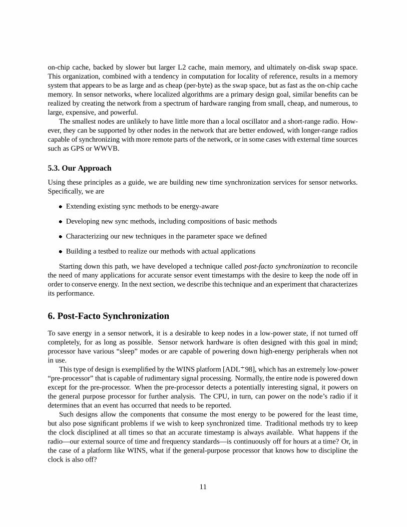
on-chip cache, backed by slower but larger L2 cache, main memory, and ultimately on-disk swap space.This organization, combined with a tendency in computation for locality of reference, results in a memorysystem that appears to be as large and as cheap (per-byte) as the swap space, but as fast as the on-chip cachememory. In sensor networks, where localized algorithms are a primary design goal, similar benefits can berealized by creating the network from a spectrum of hardware ranging from small, cheap, and numerous, tolarge, expensive, and powerful.

The smallest nodes are unlikely to have little more than a local oscillator and a short-range radio. How-ever, they can be supported by other nodes in the network that are better endowed, with longer-range radioscapable of synchronizing with more remote parts of the network, or in some cases with external time sourcessuch as GPS or WWVB.

5.3. Our Approach

Using these principles as a guide, we are building new time synchronization services for sensor networks.Specifically, we are

� Extending existing sync methods to be energy-aware

� Developing new sync methods, including compositions of basic methods

� Characterizing our new techniques in the parameter space we defined

� Building a testbed to realize our methods with actual applications

Starting down this path, we have developed a technique called post-facto synchronization to reconcilethe need of many applications for accurate sensor event timestamps with the desire to keep the node off inorder to conserve energy. In the next section, we describe this technique and an experiment that characterizesits performance.

6. Post-Facto Synchronization

To save energy in a sensor network, it is a desirable to keep nodes in a low-power state, if not turned offcompletely, for as long as possible. Sensor network hardware is often designed with this goal in mind;processor have various “sleep” modes or are capable of powering down high-energy peripherals when notin use.

This type of design is exemplified by the WINS platform [ADL�

98], which has an extremely low-power“pre-processor” that is capable of rudimentary signal processing. Normally, the entire node is powered downexcept for the pre-processor. When the pre-processor detects a potentially interesting signal, it powers onthe general purpose processor for further analysis. The CPU, in turn, can power on the node’s radio if itdetermines that an event has occurred that needs to be reported.

Such designs allow the components that consume the most energy to be powered for the least time,but also pose significant problems if we wish to keep synchronized time. Traditional methods try to keepthe clock disciplined at all times so that an accurate timestamp is always available. What happens if theradio—our external source of time and frequency standards—is continuously off for hours at a time? Or, inthe case of a platform like WINS, what if the general-purpose processor that knows how to discipline theclock is also off?

11

Our solution to this problem is post-facto synchronization. In our scheme, nodes’ clocks are normallyunsynchronized. When a stimulus arrives, each node records the time of the stimulus with respect to its ownlocal clock. Immediately afterwards, a “third party” node—acting as a beacon—broadcasts a synchroniza-tion pulse to all nodes in the area using its radio. Nodes that receive this pulse use it as an instantaneoustime reference and can normalize their stimulus timestamps with respect to that reference.

This kind of synchronization is not applicable in all situations, of course: it is limited in scope to thetransmit range of the beacon and creates only an “instant” of synchronized time. This makes it inappropriatefor an application that needs to communicate a timestamp over long distances or times. However, it doesprovide exactly the service necessary for beam-forming applications, localization systems, and other situa-tions in which we need to compare the relative arrival times of a signal at a set of spatially local detectors.

6.1. Expected Sources of Error

There are three main factors that affect the accuracy and precision achievable by post-facto synchroniza-tion. Roughly in order of importance, they are: receiver clock skew, variable delays in the receivers, andpropagation delay of the synchronization pulse.

� Skew in the receivers’ local clocks. Post-facto synchronization requires that each receiver accu-rately measure the interval that elapses between their detection of the event and the arrival of thesynchronization pulse. However, nodes’ clocks do not run at exactly the same rate, causing error inthat measurement. Since clock skew among the group will cause the achievable error bound to decayas time elapses between the stimulus and pulse, it is important to minimize this interval.

One way of reducing this error is to use NTP to discipline the frequency of each node’s oscillator.This exemplifies our idea of multi-modal synchronization. Although running NTP “full-time” defeatsone of the original goals of keeping the main processor or radio off, it can still be useful for frequencydiscipline (much more so than for phase correction) at very low duty cycles.

� Variable delays on the receivers. Even if the synchronization signal arrives at the same instantat all receivers, there is no guarantee that each receiver will detect the signal at the same instant.Nondeterminism in the detection hardware and operating system issues such as variable interruptlatency can contribute unpredictable delays that are inconsistent across receivers. The detection ofthe event itself (audio, seismic pulses, etc.) may also have nondeterministic delays associated with it.These delays will contribute directly to the synchronization error.

Our design avoids error due to variable delays in the sender by considering the sender of the syncpulse to be a “third party.” That is, the receivers are considered to be synchronized only with eachother, not with the beacon.

It is interesting to note that the error caused by variable delay is the same irrespective of the timeelapsed between the event and the sync pulse. This is in contrast to error due to clock skew that growsover time.

� Propagation delay of the synchronization pulse. Our method assumes that the synchronizationpulse is an absolute time reference at the instant of its arrival—that is, that it arrives at every node atexactly the same time. In reality, this is not the case due to the finite propagation speed of RF signals.Synchronization will never be achievable with accuracy better than the difference in the propagationdelay between the various receivers and the synchronization beacon.

12

This source of error makes our technique most useful when comparing arrival times of phenomenathat propagate much more slowly than RF, such as audio. The six-order-of-magnitude difference inthe speed of RF and audio has been similarly exploited in the past in systems such as the ORL’s ActiveBat [WJH97] and Girod’s acoustic rangefinder [Gir00].

6.2. Empirical Study

We designed an experiment to characterize the performance of our post-facto synchronization scheme. Theexperiment attempts to measure the sources of error described in the previous section by delivering a stimu-lus to each receiver at the same instant, and asking the receivers to timestamp the arrival time of that stimuluswith respect to a synchronization pulse delivered via the same mechanism. Ideally, if there are no variabledelays in the receivers or skew among the receivers’ local oscillators, the times reported for the stimulusshould be identical. In reality, these sources of error cause the dispersion among the reported times to growas more time elapses between the stimulus and the sync pulse. The decay in the error bound should happenmore slowly if NTP is simultaneously used to discipline the frequency of the receivers’ oscillators.

We realized this experiment with one sender and ten receivers, each of which was ordinary PC hardware(Dell OptiPlex GX1 workstations) running the RedHat Linux operating system. Each stimulus and syncpulse was a simple TTL logic signal sent and received by the standard PC parallel port.2 In each trial, eachreceiver reported its perceived elapsed time between the stimulus and synchronization pulse according tothe system clock, which has

���sec resolution. We defined the dispersion to be the standard deviation from

the mean of these reported values. To minimize the variable delay introduced by the operating system,the times of the incoming pulses were recorded by the parallel port interrupt handler using a Linux kernelmodule.

In order to understand how dispersion is affected by the time elapsed between stimulus and sync pulse,we tested the dispersion for 21 different values of this elapsed time, ranging from

��� �sec to

����� �sec (

��� �sec

to 16.8 seconds). For each elapsed-time value, we performed 50 trials and reported the mean. These 1,050trials were performed in a random order over the course of one hour to minimize the effects of systematicerror (e.g. changes in network activity that affect interrupt latency).

For comparison, this entire experiment was performed in three different configurations:

1. The experiment was run on the “raw clock”: that is, while the receivers’ clocks were not disciplinedby any external frequency standard.

2. An NTPv3 client was started on each receiver and allowed to synchronize (via Ethernet) to our lab’sstratum-1 GPS clock for ten days. The experiment was then repeated while NTP was running.

3. NTP’s external time source was removed, and the NTP daemon was allowed to free-run for severaldays using its last-known estimates of the local clock’s frequency. The experiment was then repeated.

To compare our post-facto method to the error bound achievable by NTP alone, we recorded two dif-ferent stimulus-arrival timestamps when running the experiment in Configuration 2: the time with respectto the sync pulse and the time according to the NTP-disciplined local clock. Similar to the other configura-tions, a dispersion value for NTP was computed for each stimulus by computing the standard deviation fromthe mean of the reported timestamps. The horizontal line in Figure 1 is the mean of those 1,050 dispersionvalues—101.70

�sec.

2This was accomplished using the author’s parallel port pin programming library for Linux, parapin, which is freely availableat http://www.circlemud.org/jelson/software/parapin

13

Pulse with NTP-trained clockPulse with Active NTP

Undisciplined Local ClockNTP Alone

Time Elapsed between Event and Synchronization (seconds)

Pre

cisi

onof

Syn

chro

niza

tion

(mic

rose

cond

s)

1001010.10.010.0010.00011e-05

1000

100

10

1

0.1

Figure 1: Synchronization error using post-facto time synchronization without external frequency discipline, withdiscipline from an active NTP time source, and with free-running NTP discipline (external time source removedafter the oscillator’s frequency was estimated). These are compared to the error bound achievable with NTP alone(the horizontal line near

�������sec). The breakpoint seen near 50msec is where error due to clock skew, which grows

proportionally with the time elapsed from stimulus to sync pulse, overcomes other sources of error that are independentof this interval. Each point represents the dispersion experienced among 10 receivers, averaged over 50 trials.

Our results are shown in Figure 1. 3

6.3. Discussion

The results shown in Figure 1 illuminate a number of aspects of the system. First, the experiment givesinsight into the nature of its error sources. The results with NTP-disciplined clock case are equivalent toundisciplined clocks when the interval is less than ��� � msec, suggesting that the primary source of errorin these cases is variable delays on the receiver (for example, due to interrupt latency or the sampling ratein the analog-to-digital conversion hardware in the PC parallel port). Beyond 50msec, the two experimentsdiverge, suggesting that clock skew becomes the primary source of error at this point.

Overall, the performance of post-facto synchronization was quite good. When NTP was used to dis-cipline the local oscillator’s frequency, an error bound very near to the clock’s resolution of

���sec was

achieved. This is significantly better than the��� � �

sec achieved by NTP alone. Clearly, the combinationof NTP’s frequency estimation with the sync pulse’s instantaneous phase correction was very effective. In-deed, the multi-modal combination’s maximum error is better than either mode can achieve alone. We findthis a very encouraging indicator for the multi-modal synchronization framework we proposed at the end ofSection 5.

Without NTP discipline, the post-facto method still performs reasonably well for short intervals betweenstimulus and sync pulse. For longer intervals, we are at the mercy of happenstance: the error depends onthe natural frequencies of whatever oscillators we happen to have in our receiver set.

3“The joy of engineering is to find a straight line on a double logarithmic diagram.” –Thomas Koenig

14

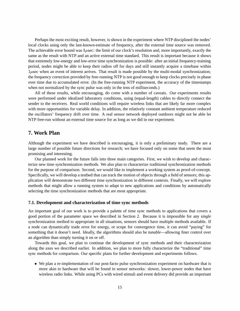
Perhaps the most exciting result, however, is shown in the experiment where NTP disciplined the nodes’local clocks using only the last-known-estimate of frequency, after the external time source was removed.The achievable error bound was

���sec: the limit of our clock’s resolution and, more importantly, exactly the

same as the result with NTP and an active external time standard. This result is important because it showsthat extremely low-energy and low-error time synchronization is possible: after an initial frequency-trainingperiod, nodes might be able to keep their radios off for days and still instantly acquire a timebase within���

sec when an event of interest arrives. That result is made possible by the multi-modal synchronization;the frequency correction provided by free-running NTP is not good enough to keep clocks precisely in phaseover time due to accumulated error. (In the free-running NTP experiment, the accuracy of the timestampswhen not normalized by the sync pulse was only in the tens of milliseconds.)

All of these results, while encouraging, do come with a number of caveats. Our experiments resultswere performed under idealized laboratory conditions, using (equal-length) cables to directly connect thesender to the receivers. Real world conditions will require wireless links that are likely far more complexwith more opportunities for variable delay. In addition, the relatively constant ambient temperature reducedthe oscillators’ frequency drift over time. A real sensor network deployed outdoors might not be able letNTP free-run without an external time source for as long as we did in our experiment.

7. Work Plan

Although the experiment we have described is encouraging, it is only a preliminary study. There are alarge number of possible future directions for research; we have focused only on some that seem the mostpromising and interesting.

Our planned work for the future falls into three main categories. First, we wish to develop and charac-terize new time synchronization methods. We also plan to characterize traditional synchronization methodsfor the purpose of comparison. Second, we would like to implement a working system as proof-of-concept.Specifically, we will develop a testbed that can track the motion of objects through a field of sensors; this ap-plication will demonstrate two different time synchronization in different contexts. Finally, we will exploremethods that might allow a running system to adapt to new applications and conditions by automaticallyselecting the time synchronization methods that are most appropriate.

7.1. Development and characterization of time sync methods

An important goal of our work is to provide a palette of time sync methods to applications that covers agood portion of the parameter space we described in Section 2. Because it is impossible for any singlesynchronization method to appropriate in all situations, sensors should have multiple methods available. Ifa node can dynamically trade error for energy, or scope for convergence time, it can avoid “paying” forsomething that it doesn’t need. Ideally, the algorithms should also be tunable—allowing finer control overan algorithm than simply turning it on or off.

Towards this goal, we plan to continue the development of sync methods and their characterizationalong the axes we described earlier. In addition, we plan to more fully characterize the “traditional” timesync methods for comparison. Our specific plans for further development and experiments follows.

� We plan a re-implementation of our post-facto pulse synchronization experiment on hardware that ismore akin to hardware that will be found in sensor networks: slower, lower-power nodes that havewireless radio links. While using PCs with wired stimuli and event delivery did provide an important

15

proof-of-concept and encouraging results, we wish to investigate the effects on error of factors such asslower clock speeds, variable latency of radios, and nondeterminism introduced by radio propagationanomalies. We plan to do these tests using the wireless sensor network testbed in place as part of therelated SCADDS project [EGHK99, CEE

�

01].

There are many interesting dimensions of pulse synchronization that we did not explore with ourinitial experiment. For example, what are the effects on error of scaling up the number of nodes,the duty cycle of the nodes, or changes in the ambient temperature? Many of these questions can beanswered with a larger, truly untethered testbed.

An even a more basic question that we would like to answer is: what is the best modality for a syn-chronization pulse? We should not assume that a radio signal is the best (e.g., most deterministicallydetected) mode. We plan a simple experiment to test the detection determinism of other modes notyet examined, such as using a strobe light to trigger remote photodiodes. By using a multichanneloscilloscope to compare the dispersion in triggering times of various modes (e.g., the strobe light,radios with various MAC layers, and wired stimuli), we can get an interesting picture of how thedetection modalities themselves contribute to the overall system’s error budget.

� Additional (related) time-synchronization methods will be developed based on the existing primitives.Specifically, we wish to investigate synchronization pulse chaining. Pulse chaining is an extensionto the pulse sync method we described earlier. Standard pulse synchronization is only effective forcreating a synchronized timebase within the transmit radius of a single beacon. However, if certainreceivers “relay” the pulse—retransmitting it to a new set of receivers outside the range of the originalbeacon—the scope of the timebase can be expanded. The pulse may be relayed many times to makethe scope of the timebase larger and larger.

Naturally, each link in this synchronization chain will accumulate error. Our plan is to understandhow this error accumulates as the size of the synchronized area increases. This “maximum error vs.distance” is analogous to the “maximum error vs. time” experiment we described in Section 6.

� We will characterize some existing methods for acquiring time along the same axes (such as scope,maximum error, lifetime, etc.) that we have used to evaluate our own time sync methods. This willallow a for a more informed comparison of our methods with related work in the area. Our exper-iment’s comparison of pulse synchronization with NTP is one example of this kind of comparison;we would like to make similar statements with respect to systems such as GPS, WWV/WWVB, andGPS-via-CDMA.

7.2. Testbed implementation as proof-of-concept

Although experiments that characterize our methods are important, we also think it is important to imple-ment an actual application using these methods as a proof-of-concept. Therefore, the second major portionof our planned work is the implementation of a testbed that demonstrates our time sync algorithms in thecontext of a sensing application.

Our proposed testbed application is tracking of cooperative objects through a sensor field. A “cooper-ative” object is one that wants to be tracked; that is, the object has been augmented in a way that makes iteasier to localize. The goal is to build sensor network that will report to a user the location and speed ofthe cooperative object over time. The sensor field will be truly distributed: that is, its geographic span willprevent any single node from broadcasting a radio message globally.

16

The application we propose will build on Girod’s prototype acoustic rangefinder [Gir00]. His rangefinderuses digital signal processing techniques to accurately determine the time of arrival of a specially formedsound. (The sound is a “chirp” that is modulated by a sender to make it more easily detected by the receiver.)If the sender and receiver are synchronized in time, Girod’s technique allows accurate determination of thetime of flight of sound between two points. This, in turn, leads to an accurate range estimate between them.

In cooperation with Girod, we plan to use post-facto time synchronization to facilitate measurement ofthe time of flight of sound from an audio source to a set of receivers—not just a single receiver—allowingthem to trilaterate. At any given instant, this technique will report instantaneous position in a coordinatesystem defined by the sensors4 . As the object moves through the sensor field, many such localizationmeasurements can be taken and integrated to form an estimate of velocity.

This experiment demonstrates two aspects of our time synchronization services:

� Post-facto synchronization. The post-facto sync we have developed (as described earlier in this paper)allows a localized set of receivers to create an ephemeral synchronization with a maximum error of���

sec. This is exactly what the trilateration/localization service needs.

� Pulse chaining. In order to integrate a series of these localization measurements over time, the sensorsmust be able to share a timebase that is wider in scope and longer in lifetime. However, since theobject will be moving relatively slowly, the maximum error constraint is considerably weaker (e.g.,on the order of 10’s or even 100’s of milliseconds). Pulse chaining makes exactly this tradeoff:chaining together a series of local, ephemeral timebases into a larger-scope and longer-lasting one, atthe expense of accumulated error.

We believe this experiment to be an effective demonstration on several fronts:

� Even an single application can often have a variety of time-sync needs.

� Meeting these disparate needs by using a variety of time-sync methods results in a more energy-efficient and less expensive system than a single sync method that would be forced to meet the unionof all requirements.

� Sensor nodes can sometimes achieve advanced time-sync without the need for additional specializedhardware.

7.3. Exploration of methods for tuning and automatic modality selection

There are additional future directions that we wish to pursue, though time may not permit a completeexploration of these details in the context of an actual implementation. We plan to examine some of theseissues in the context of simulation or modeling instead. Specifically:

� Our vision is that nodes can save energy by selecting a time synchronization method that is bothnecessary and sufficient for its needs. Ideally, those methods should also be tunable—allowing finercontrol over an algorithm than simply turning it on or off. Tunability will allow applications to tailora sync method, making the gap between what’s needed and what’s provided even smaller. Through

4In this experiment, we assume that each sensor is preprogrammed with its position in some global coordinate system. Inthe context of a testbed meant to demonstrate time synchronization, this assumption is a reasonable one. In parallel, Girod isdeveloping techniques that allow a distributed federation of sensors to dynamically create a self-consistent coordinate system.

17

some simple experimentation or simulation, we would like to study the gains that might be realizedthrough tuning.

One such “tuning knob” that might be possible is in selecting the number of nodes that participatein a federation of synchronized nodes. Many time-standards (e.g., UTC(USNO), the U.S. NavalObservatory’s realization of UTC), use a large ensemble of clocks and dynamically choose the best inorder to improve precision. Will adding additional beacons make post-facto synchronization better,at the expense of more energy expended by the additional nodes that are participating? If so, this isanother interesting energy-error tradeoff.

� Until now, we have assumed that a palette of sync methods are available to applications, and the exactmethod used is selected by the system designer at design-time. Is it possible for the system to adaptby dynamically selecting the best algorithm while it’s running? Is it possible for an application toautomatically turn the tuning knobs described earlier?

8. Conclusions

Time synchronization is a critical piece of infrastructure for any distributed system. Distributed, wirelesssensor networks make heavy use of synchronized time, but often have unique requirements in the scope,lifetime, and maximum error of the synchronization achieved, as well as the time and energy required toachieve it. Existing time synchronization methods need to be extended to meet these new needs.

We have presented an implementation of our own sensor network time synchronization scheme, post-facto synchronization. This method combines the oscillator frequency discipline provided by NTP withan instantaneous phase correction provided by a simple synchronization signal sent by a beacon. Ourexperiments have shown timing error for a group of 10 nodes to be bounded near the limit of our clockresolution of

���sec.

An important additional result is that the same error bound was achieved even when NTP no longer hadan active external time or frequency standard, after an initialization period when it was allowed to estimatethe local oscillator’s frequency error. This is critical for sensor networks where limited energy reserves andthe high energy cost of operating a wireless radio make standard NTP unsuitable for long-lived, low-poweroperation.

Although our current results are a preliminary laboratory study, we believe that post-facto synchro-nization over wireless radios will be able to support the same instantaneous creation of a short-lived butlow-error synchronized timebase ever after a long period of radio silence. We propose ongoing researchwhere we can

� Move our experiment from the lab to real sensor network nodes, and develop additional methods;

� Characterize our methods, and traditional methods, according to appropriate metrics for comparison;

� Prove these methods are applicable to real systems by building an application testbed; and

� Explore additional issues such as tuning and voting through simulation and modeling.

Acknowledgments

Portions of this work were supported by DARPA under grant No. DABT63-99-1-0011 as part of theSCADDS project, and was also made possible in part due to support from Cisco Systems.

18

References

[ADL�

98] G. Asada, M. Dong, T.S. Lin, F. Newberg, G. Pottie, W.J. Kaiser, and H.O. Marcy. WirelessIntegrated Network Sensors: Low Power Systems on a Chip. In Proceedings of the EuropeanSolid State Circuits Conference, 1998.

[APK00] A.A. Abidi, G.J. Pottie, and W.J. Kaiser. Power-conscious design of wireless circuits andsystems. Proceedings of the IEEE, 88(10):1528–45, October 2000.

[BD82] Ian R. Bartky and Steven J. Dick. The first north american time ball. Journal for the Historyof Astronomy, 13:50–54, 1982.

[BGS01] Ph. Bonnet, J. Gehrke, and P. Seshadri. Towards sensor database systems. In Proceedings ofthe 2nd International Conference on Mobile Data Management, Hong Kong, January 2001.

[CEE�

01] Alberto Cerpa, Jeremy Elson, Deborah Estrin, Lewis Girod, Michael Hamilton, and JerryZhao. Habitat monitoring: Application driver for wireless communications technology. InProceedings of the 2001 ACM SIGCOMM Workshop on Data Communications in Latin Amer-ica and the Caribbean, April 2001.

[Cri89] Flaviu Cristian. Probabilistic clock synchronization. Distributed Computing, 3:146–158, 1989.

[DGT96] Donald T. Davis, Daniel E. Geer, and Theodore Ts’o. Kerberos with clocks adrift: History,protocols, and implementation. Computing Systems, 9(1):29–46, Winter 1996.

[EGHK99] Deborah Estrin, Ramesh Govindan, John Heidemann, and Satish Kumar. Next centurychallenges: Scalable coordination in sensor networks. In Proceedings of the fifth annualACM/IEEE international conference on Mobile computing and networking, pages 263–270,1999.

[Gir00] Lewis Girod. Development and characterization of an acoustic rangefinder. Technical Report00-728, University of Southern California, Department of Computer Science, March 2000.

[GZ89] R. Gusell and S. Zatti. The accuracy of clock synchronization achieved by TEMPO in BerkeleyUNIX 4.3 BSD. IEEE Transactions on Software Engineering, 15:847–853, 1989.

[Hil] Jason Hill. A security architecture for the post-pc world. U.C. Berkeley Technical Report, toappear.

[HSW�

] Jason Hill, Robert Szewczyk, Alec Woo, Seth Hollar, David Culler, and Kristofer Pister. Sys-tem architecture directions for networked sensors. U.C. Berkeley Technical Report, to appear.

[IGE00] Chalermek Intanagonwiwat, Ramesh Govindan, and Deborah Estrin. Directed diffusion: Ascalable and robust communication paradigm for sensor networks. In Proceedings of the SixthAnnual International Conference on Mobile Computing and Networking, pages 56–67, Boston,MA, August 2000. ACM Press.

[Kap96] Elliott D. Kaplan, editor. Understanding GPS: Principles and Applications. Artech House,1996.

19

[KKP99] J.M. Kahn, R.H. Katz, and K.S.J. Pister. Next century challenges: mobile networking forSmart Dust. In Proceedings of the fifth annual ACM/IEEE international conference on Mobilecomputing and networking, pages 271–278, 1999.

[Lam78] Leslie Lamport. Time, clocks, and the ordering of events in a distributed system. Communi-cations of the ACM, 21(7):558–65, 1978.

[Lan83] David S. Landes. Revolution in Time: Clocks and the Making of the Modern World. BelknapPress, 1983.

[LL99] Kristine Larson and Judah Levine. Time transfer using the phase of the gps carrier. IEEETransactions On Ultrasonics, Ferroelectrics and Frequency Control, 46:1001–1012, 1999.

[LS96] Henrik Lonn and Rolf Snedsbøl. Efficient synchronisation, atomic broadcast and membershipagreement in a TDMA protocol. Technical report, CTH, Dept. of Computer Engineering,Laboratory for Dependable Computing (LDC), 1996.

[LSW91] B. Liskov, L. Shrira, and J. Wroclawski. Efficient at-most-once messages based on synchro-nized clocks. ACM Trans. on Computer Sys., Special Section on Communication Architecturesand Protocols, 9(2):125, May 1991.

[Mil94] David L. Mills. Internet Time Synchronization: The Network Time Protocol. In ZhonghuaYang and T. Anthony Marsland, editors, Global States and Time in Distributed Systems. IEEEComputer Society Press, 1994.

[MKMT99] J. Mannermaa, K. Kalliomaki, T. Mansten, and S. Turunen. Timing performance of variousGPS receivers. In Proceedings of the 1999 Joint Meeting of the European Frequency and TimeForum and the IEEE International Frequency Control Symposium, pages 287–290, April 1999.

[MMK99] D.N. Matsakis, M. Miranian, and P. Koppang. Steering the U.S. Naval Observatory (USNO)Master Clock. In Proceedings of the Institute of Navigation National Technical Meeting: Vi-sion 2010, Present and Future, January 1999.

[PK00] G.J. Pottie and W.J. Kaiser. Wireless integrated network sensors. Communications of the ACM,43(5):51–58, May 2000.

[PWB�

87] G. Popek, B. Walker, D. Butterfield, R. English, C. Kline, G. Thiel, and T. Page. Functionalityand architecture of the LOCUS distributed file system. In Bharat K. Bhargava, editor, Con-currency Control and Reliability in Distributed Systems. Van Norstrand Reinhold (New York,NY), 1987. Also published in ACM SOSP-9, Bretton Woods NH, Oct. 1982.

[SA98] Dava Sobel and William J.H. Andrewes. The Illustrated Longitude. Walker & Co., 1998.

[SNS88] Jennifer G. Steiner, Clifford Neuman, and Jeffrey I. Schiller. Kerberos: An authenticationservice for open network systems. In USENIX Association, editor, USENIX Conference Pro-ceedings (Dallas, TX, USA), pages 191–202, Berkeley, CA, USA, Winter 1988. USENIX As-sociation.

[Soh00] Katayoun Sohrabi. On Low Power Self Organizing Sensor Networks. PhD thesis, Universityof California, Los Angeles, 2000.

20

[SPK00] W. Schaefer, A. Pawlitzki, and T. Kuhn. New trends in two-way time and frequency transfervia satellite. In Proceedings of the 31st Annual Precise Time and Time Interval (PTTI) Systemsand Applications Meeting, 2000.

[ST87] T. K. Srikanth and Sam Toueg. Optimal clock synchronization. J-ACM, 34(3):626–645, July1987.

[Tho97] C. Thomas. The accuracy of the international atomic timescale TAI. In Proceedings of the11th European Frequency and Time Forum, pages 283–289, 1997.

[WJH97] A. Ward, A. Jones, and A. Hopper. A new location technique for the active office. IEEEPersonal Communications, 4(5):42–47, October 1997.

[YHR�

98] K. Yao, R.E. Hudson, C.W. Reed, D. Chen, and F. Lorenzelli. Blind beamforming on a ran-domly distributed sensor array system. IEEE Journal of Selected Areas in Communications,16(8):1555–1567, Oct 1998.

21