time series of physical and optical parameters off shimane

Journal of Oceanography, Vol. 53, pp. 245 to 258. 1997

245Copyright The Oceanographic Society of Japan.

Time Series of Physical and Optical Parameters offShimane, Japan, during Fall of 1993: First Observation byMoored Optical Buoy System for ADEOS Data Verification

J. ISHIZAKA1, I. ASANUMA2, N. EBUCHI3, H. FUKUSHIMA4, H. KAWAMURA3, K. KAWASAKI5,M. KISHINO6, M. KUBOTA7, H. MASUKO8, S. MATSUMURA9, S. SAITOH10, Y. SENGA7,M. SHIMANUKI11, N. TOMII12 and M. UTASHIMA13

1National Institute for Resources and Environment, 16-3 Onogawa, Tsukuba, Ibaraki 305, Japan2Japan Marine Science and Technology Center, 2-15 Natsushima-machi, Yokosuka, Kanagawa 237, Japan3Faculty of Science, Tohoku University, Aoba, Aramaki, Sendai, Miyagi 980, Japan4School of High-Technology for Human Welfare, Tokai University, 317 Nishino, Numazu, Shizuoka 410-03, Japan5National Research Institute of Fisheries Science, 2-12-4 Fukuura, Kanazawa, Yokohama, Kanagawa 236, Japan6The Institute of Physical and Chemical Research, 2-1 Hirosawa, Wako, Saitama 351-01, Japan7School of Marine Science and Technology, Tokai University, 3-20-1 Orido, Shimizu, Shizuoka 424, Japan8Communication Research Laboratory, 893-1 Hirai, Kashima, Kashima, Ibaraki 314, Japan9National Research Institute of Far Seas Fisheries, 5-7-1 Orido, Shimizu, Shizuoka 424, Japan10Faculty of Fisheries, Hokkaido University, 3-1-1 Minato-machi, Hakodate, Hokkaido 041, Japan11Japan Weather Association, 2-9-2 Kandanishiki, Chiyoda, Tokyo 101, Japan12Remote Sensing Technology Center, 1401 Ohashi Numanoue, Hatoyama, Hiki, Saitama 350-03, Japan13National Space Development Agency of Japan, 2-1-1 Sengen, Tsukuba, Ibaraki 305, Japan

(Received 26 June 1996; in revised form 18 October 1996; accepted 24 October 1996)

A moored optical buoy system has been developed by the National Space DevelopmentalAgency of Japan (NASDA) for verification of the ocean-observing sensors of the AdvancedEarth Observation Satellite (ADEOS). The buoy was operated from August 25 toNovember 26, 1993, in the Japan Sea, off Shimane, Japan. Three-months time series ofphysical parameters indicate that the decrease of insolation and increase of wind velocitycaused cooling of the sea surface and deepening of the mixed layer. The optical measurementsystems of the buoy are still underdeveloped, and the experiment indicated several pointsthat have to be improved. However, chlorophyll a concentrations, estimated from upwardradiance and downward irradiance at 1.8-m depth, are generally consistent with thechlorophyll fluorescence measured by a fluorometer of the buoy system. The time changeof the chlorophyll a concentration showed a gradual increase during October and adecrease in November. Simple calculations of enrichment of the mixed layer and criticaldepth theory could explain the fall bloom. Sea surface temperature showed a goodcorrelation with coincident AVHRR/NOAA-12 MCSST data. Wind speed and directionand wave height also showed good correlations with ERS-1/AMI and TOPEX/POSEIDONdata. The optical buoy system is useful for both verification of satellite data andunderstanding the time changes of physical and biological parameters.

1. IntroductionThe Advanced Earth Observing Satellite (ADEOS)

with eight earth observation sensors was launched on Au-gust 17, 1996 by the National Space Development Agencyof Japan (NASDA). The Ocean Color and TemperatureSensor (OCTS) provides ocean chlorophyll a concentrationfrom upward radiance and sea surface temperature and the

NASA Scatterometer (NSCAT) measures wind speed andwind direction. The first test data from these sensors weresuccessfully received. It is necessary to verify the data fromthese ocean remote sensors with an appropriate data setobtained in situ in order to use the satellite data. However,it is not easy to collect sufficient data to verify those oceanremote sensors. Specifically, sporadic ship observations are

Keywords:⋅Optical buoy,⋅ Japan Sea,⋅ocean color,⋅ remote sensing,⋅ sea surfacetemperature,

⋅ scatterometer,⋅wind,⋅mixed layer,⋅phytoplanktonbloom.

246 J. Ishizaka et al.

not enough for the verification of large-area and long-periodsatellite observations.

An optical mooring system is also a useful tool foroceanography. It can measure detailed time variations, whichare difficult to observe by ship or satellite. Ocean mooredbuoy systems provide continuous observations of the vari-ables that are required for calibration and verification ofsatellite remote sensing. Sea surface temperatures measuredby NOAA/AVHRR satellites have been validated with seasurface temperature data obtained by moored buoy systems(McClain et al., 1985; Sakaida and Kawamura, 1992). Seasurface wind and wave height obtained by TOPEX/POSEIDON and ERS-1/AMI have been also verified bybuoy data (Ebuchi and Kawamura, 1994).

The Coastal Zone Color Scanner (CZCS) is the onlypreviously operated ocean color sensor for phytoplanktonpigments. The data were verified with ship observed upwardradiance and phytoplankton pigment concentrations invarious areas (cf. Smith and Baker, 1982; Gordon et al., 1983).However, the verification did not have globally spatial norcontinuous time coverage. Specifically, both ship-observedphytoplankton pigment concentrations and upward radiances,as well as CZCS data, were too sporadic for verification ofthe CZCS data around Japan (Ishizaka and Harashima,1991). A few comparisons indicated that there are difficultieswith the atmospheric correction algorithm in the region(Ishizaka et al., 1992; Fukushima and Ishizaka, 1993). Fur-thermore, analysis of the data from clear atmosphere andclear water regions indicates a significant temporal variationin the calibration factors (Evans and Gordon, 1994). Recently,moored optical buoy systems have been developed (cf.Dickey et al., 1991; Smith et al., 1991), and calibration andverification of ocean color satellite data by optical mooringsystems have been suggested (Mueller and Austin, 1995).

NASDA has developed an optical moored buoy systemthat is specifically designed for verification of sea surfacetemperature and ocean color of OCTS, and wind speed anddirection of NSCAT on ADEOS (Matsumura et al., 1992).The NASDA buoy system was deployed for three months,in the fall of 1993, off Shimane, Japan. Here we describe theresults of the time changes of physical parameters and fluxcalculation with the data, and biological parameters andsimple explanation of the changes. We further describe theresults of verifications of sea surface temperature fromNOAA-12/AVHRR and sea wind speed and direction ob-tained by ERS-1 and TOPEX using the NASDA buoysystem. Additionally, we have verified wave height obser-vations of TOPEX.

2. Optical Moored Buoy SystemThe buoy system was originally developed by the

Japan Marine Fisheries Resources Exploitation Center(JAMFREC) for monitoring resources for fisheries(JAMFREC, 1990, 1991; Ichikawa et al., 1992; Saitoh et al.,

1992) and was modified by OCTS/NSCAT mission teams(Matsumura et al., 1992). The specification of the buoysystem is shown in Table 1 and Fig. 1. Atmospheric tem-perature, pressure, humidity, and wave height as well aswind speed and direction were obtained by the buoy system.Sea water temperatures were measured by thermistors atbuoy depths of 1 m and 6.5 m, and additional thermistorswere attached at 25, 50, and 100 m on the mooring chain.Wave height and direction were also measured. Instrumentsto measure those meteorological and physical oceanographicparameters were originally fitted to the JAMFREC buoysystem.

The measurements of optical and biological parametersshould be considered from the point of verification of oceancolor. Phytoplankton pigment estimation by ocean colorremote sensing is basically composed of two different al-gorithms; an atmospheric correction algorithm and an in-water algorithm (cf. Gordon and Morel, 1983). The atmo-spheric correction algorithm is used to obtain sea surfaceupward radiance from the satellite detected radiance, andphytoplankton pigments and other water properties, includingchlorophyll a, are estimated from the sea surface upwardradiance by the in-water algorithm. Thus, one requires toverify both sea surface upward radiance and specific vari-ables in order to verify the products of OCTS. The NASDA

Fig. 1. Diagram of the NASDA moored optical buoy system.

Time Series of Physical and Optical Parameters off Shimane, Japan, during Fall of 1993 247

buoy system measured, two layers of upward radiance anddownward irradiance spectrally in order to estimate theupward radiance from the sea surface. In vivo chlorophyllfluorescence was also measured by a fluorometer. It isknown that the chlorophyll fluorescence varies with thephysiological and taxonomic conditions of phytoplankton;however, it is useful for qualitative comparisons betweensatellite-estimated and radiometer-estimated chlorophyll aconcentrations.

Two underwater upward and downward radiometerswere placed at depths of 1.8 m and 6.8 m (Fig. 1). Thecollector parts of the radiometers were extended from thecenter of the buoy system in order to avoid shelf shadowing,with 3-m and 1.2-m arms at the top and bottom, respectively.These radiometers were specifically designed for this opticalbuoy system, and a fiber optical system was adopted tocollect the upward radiance and downward irradiance. Theoptical energy from 400 to 800 nm was separated into 2-nmbands by the spectrograph and measured by a linear image

array detector. Chlorophyll fluorescence was monitored byan Aquatracka-III fluorometer placed at the bottom of thebuoy system. In order to avoid degrading optical signals bybio-fouling, the surfaces of the optical sensors were cleanedby brushing systems, which are similar to the one used byFukuchi et al. (1988).

The buoy system stored data every hour for meteoro-logical variables and sea surface temperature. The opticalsignals were taken every hour from 8:00 a.m. to 4:00 p.m.and every 20 min. from 10:00 a.m. to 2:00 p.m. The systemalso transmitted part of the data in real time by the DataCollection System (DCS) of the Japanese GeostationaryMeteorological Satellite (GMS-4). The buoy system wasdeployed off Shimane, Japan (35°20′ 11.5″ N, 131°40′ 30.1″E, Fig. 2) in a water depth of 146 m from August 25 toNovember 26, 1993. A further detail description of the buoysystem will be published in the near future (NASDA, inpreparation).

Table 1. Specifications of sensors of the NASDA optical buoy.

*1) Radiance and irradiance sensors arc calibrated using a sub-standard lamp traced to National Institute of Standard (NIST).*2) Each radiance sensor equipped with a cosine collector and each irradiance sensor equipped with a Gaussian tube (FOV = 10°).*3) Each underwater optical sensor including a fluorometer equipped with a mechanical cleaner, which wipes optical windows every

3 hours.


3. Results

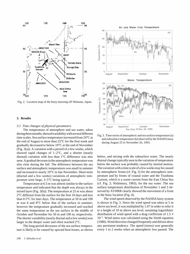
3.1 Time changes of physical parametersThe temperature of atmosphere and sea water, taken

during three months, showed variability with several differenttime scales. Sea surface temperature increased from 24°C atthe end of August to more than 25°C for the first week andgradually decreased to below 19°C at the end of November(Fig. 3(a)). A variation with a period of a few weeks, whichshowed rapid changes of 1–2°C, and a shorter (nearlydiurnal) variation with less than 1°C difference was alsoseen. A gradual decrease in the atmospheric temperature wasalso clear during the fall. The difference between the seasurface and atmospheric temperatures was small in summerand increased to nearly 10°C to late November. Short-term(diurnal and a few weeks) variations of atmospheric tem-perature were large, 3–5°C being typical.

Temperature at 6.5 m was almost similar to the surfacetemperature and indicated that the depth was always in themixed layer (Fig. 3(b)). The temperature at 25 m was about2°C different from the surface for the first 10 days and lessthan 0.5°C for later days. The temperature at 50 m and 100m was 6 and 8°C below that of the surface in summer;however the temperature gradually increased and reachedthe same temperature as the sea surface in the middle ofOctober and November for 50 m and 100 m, respectively.The shorter variability (nearly diurnal and a few weeks) waslarger in the deeper water and often reached 2°C.

The long-period decreases of the sea surface tempera-ture is likely to be caused by upward heat losses, as shown

below, and mixing with the subsurface water. The nearlydiurnal change typically seen in the variation of temperaturebelow the surface was probably caused by inertial motion.The variation with a time scale of a few weeks may be causedby atmospheric fronts (cf. Fig. 5) for the atmospheric tem-perature and by fronts of coastal water and the TsushimaCurrent, which is a warm current from the East China Sea(cf. Fig. 2; Nishimura, 1983), for the sea water. The seasurface temperature distribution of November 1 and 3 ob-served by AVHRR clearly showed the movement of a frontat the buoy location (Fig. 4).

The wind speed observed by the NASDA buoy systemis shown in Fig. 5. Since the wind speed was taken at 5 mabove sea level, it was multiplied by 1.07 in order to refer itto a height of 10 m above sea level, assuming logarithmicdistribution of wind speed with a drag coefficient of 1.5 ×10–3. Wind stress was calculated using the Smith equation(1980). Wind direction changed frequently and did not showany persistent tendency. The speed (stress) rose generallyevery 1 to 2 weeks when an atmospheric low passed. The

Fig. 2. Location map of the buoy mooring off Shimane, Japan.

Fig. 3. Time series of atmospheric and sea surface temperature (a)and subsurface temperature (b) observed by the NASDA buoyduring August 25 to November 26, 1993.


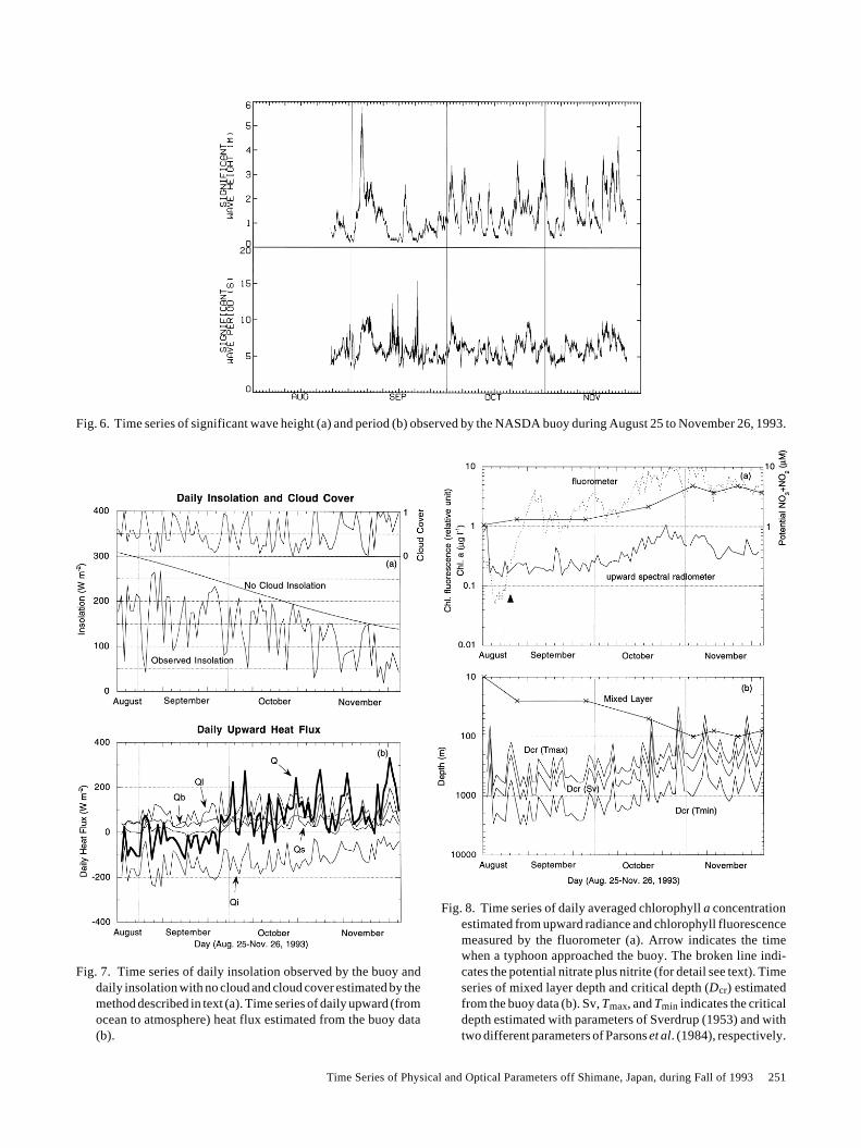
speed increased due to the monsoon in November withfluctuations having a 2–4 day period. The speed was nearly20 m s–1 and the stress exceeded 1 N m–2 on September 3–4 when a typhoon passed this area. Time changes of waveheight and periods corresponded to the variation of windspeed (Fig. 6). Wave heights greater than 5 m were recordedon September 4, when a typhoon approached the buoy. Inlate October and November, relatively high waves of 2 to 4m were observed when the winter monsoon blew.

Using these buoy data, heat flux was calculated byprocedures listed in the Appendix, mostly following Endoh(1992). Total heat flux, Q, was estimated as the sum of longwave radiation, Qb, short wave radiation, Qi, latent heat, Ql,and sensible heat Qs. By definition, the short wave radiationcorresponds to the observed insolation and is relativelylarger during September and decreased in November (Fig.7). Long wave radiation, latent heat and sensible heat mostlyshowed that the heat transferred from ocean to atmosphere.The total heat flux showed heating of the sea surface duringSeptember and cooling for the rest of the time. This temporalchange of heat flux showed that the decrease of the seasurface temperature and deepening of the mixed layer iscaused by the decrease of insolation and increase of windvelocity from the summer to winter.

3.2 Time changes of optical parametersThis is the first long-term experiment on the optical part

of the buoy system, and there were some difficulties inobtaining complete data. First, some of the clearer systems

did not function properly during the deployment. Second,the sensitivity of the optical system was not sufficient foraccurate determination of chlorophyll a from the upwardradiation. Furthermore, water samples for chlorophyll ameasurements could be taken only when the buoy wasdeployed and recovered, and underwater optical measure-ments from the ship, coincident with the buoy measurements,were not available. The first two problems were specificallyserious for 6.8-m radiometers, and it was impossible to usethe data. It was originally planned to use two radiometersplaced at 1.8 m and 6.8 m to extrapolate surface upwardradiance. Thus, here we estimated chlorophyll a from theradiance data from 1.8 m normalized by the downwardirradiance at the same depth. The error for chlorophyll acaused by using only data from 1.8 m is at present unknown.Monitoring the cleaner system of the fluorometer also indi-cated trouble with the system after the typhoon on September4.

The three-band algorithm developed by Kishino et al.(1995) was used for the estimation of chlorophyll a con-centrations from the observed upward radiance. The formulafor calculation of chlorophyll a concentration was

CHL = 0.2924((R4 + R5)/R3)3.520,

where CHL is chlorophyll a concentration (µg l–1), and R3,R4 and R5 are the upward radiance normalized by downwardirradiance integrated for OCTS band 3 (480–550 nm), 4(510–530 nm), and 5 (555–575 nm), respectively.

Fig. 4. Sea surface temperature observed by AVHRR around the buoy location on November 1 (left) and November 3 (right). Brightand dark color indicates low and high sea surface temperature, respectively. White indicates land and cloud.


The time series of chlorophyll a concentration obtainedby radiometer and chlorophyll fluorescence obtained byfluorometer is shown in Fig. 8. There was some noise mostlycaused by the low sensitivity even with the 1.8-m radiometerdata. Thus, a daily average of the data was taken afternoticeable noises were removed by visual inspection. Theobserved chlorophyll fluorescence increased during twoweeks after the typhoon (September 4) by about a factor of30. This increase was probably caused by bio-fouling afterthe trouble with the cleaner system. Time changes of chlo-rophyll a concentration and fluorescence were similar be-fore and after the typhoon. Both chlorophyll a concentrationand chlorophyll fluorescence decreased by about a factor of3 after 2–3 days from the buoy’s deployment. Both signals

were steady during late September, gradually increased inOctober, and decreased in November.

Water samples were also taken when the buoy wasdeployed and recovered, and chlorophyll a concentrationswere measured by HPLC. The surface concentrations were0.18 µg l–1 for August 25 and 0.47 µg l–1 for November 26.The concentration at the end of the experiments was similarto the value estimated by radiometer (0.4 µg l–1). However,the radiometer overestimated the initial chlorophyll a con-centration (0.8 µg l–1), and concentration in the water samplewas very similar to the value (0.2 µg l–1) estimated by theradiometer after the rapid drop of chlorophyll a after 2–3days from the buoy’s deployment. A rapid drop of chloro-phyll fluorescence was also observed and this coincided

Fig. 5. Time series of wind speed (a, b) observed by the NASDA buoy and wind stress (c) calculated from the data during August 25to November 26, 1993.


Fig. 6. Time series of significant wave height (a) and period (b) observed by the NASDA buoy during August 25 to November 26, 1993.

Fig. 7. Time series of daily insolation observed by the buoy anddaily insolation with no cloud and cloud cover estimated by themethod described in text (a). Time series of daily upward (fromocean to atmosphere) heat flux estimated from the buoy data(b).

Fig. 8. Time series of daily averaged chlorophyll a concentrationestimated from upward radiance and chlorophyll fluorescencemeasured by the fluorometer (a). Arrow indicates the timewhen a typhoon approached the buoy. The broken line indi-cates the potential nitrate plus nitrite (for detail see text). Timeseries of mixed layer depth and critical depth (Dcr) estimatedfrom the buoy data (b). Sv, Tmax, and Tmin indicates the criticaldepth estimated with parameters of Sverdrup (1953) and withtwo different parameters of Parsons et al. (1984), respectively.


with the increase of sea surface temperature on August 27,indicating a sudden change of water mass. AVHRR seasurface temperature images (cf. Fig. 4) in this area showedthe presence of frontal structures near the buoy system, andthe rapid drop of the chlorophyll a concentration wasprobably caused by the movement of the front. Comparisonof time series of sea surface temperature (Fig. 3) and chloro-phyll a concentration (Fig. 8) show a correspondence of lowtemperature and high chlorophyll a concentration in timeperiods with a scales of a few weeks. It is possible that thediscrepancy between the chlorophyll a concentrations in thewater sample and from the buoy radiometer may be the resultof sampling from different water masses separated by thefront.

The gradual increase of chlorophyll a concentrationduring October and the maximum at the end of October maybe explained in terms of the time change of mixed layerdepth. Nitrate plus nitrite concentrations observed near thebuoy system on deployment showed low concentration (~1µM) in the surface mixed layer and increased linearly from30 m to 10 µM at 100 m. Nitrate plus nitrite concentrationwithout phytoplankon uptake (hereafter, potential nitrateplus nitrate) in the mixed layer can be calculated from themixed layer depth estimated from the temperature timeseries (Fig. 8), if the high nitrate plus nitrite subsurface wateris assumed to be entrained into the mixed layer with verticalmixing. The potential nitrate plus nitrite concentration in-creased in October and reached to 5 µM in mid-November.The increase of nitrate plus nitrite concentration correspondedto the increase of chlorophyll a concentration in the mixedlayer. However, the maximum of the chlorophyll a con-centration occurred in early November and the concentrationgradually decreased during November. The nitrate plusnitrite concentration in the surface water (0–40 m) was high(3 µM) at the end of the experiment, and nutrient limitationcould not be explained from the nitrate plus nitrite con-centration.

It is expected that the decrease of insolation and in-crease of mixed layer depth may be cause by light limitationon phytoplankton growth. Sverdrup (1953) theorized thetiming of the spring bloom, in what is known as the criticaldepth theory. The critical depth is the depth where integratedprimary production balances with the integrated respirationand/or death of phytoplankton. Spring bloom initiates whenwinter deep mixed layer become shallower than the criticaldepth. Recent works related to the critical depth theory arereviewed by Ishizaka (1996). This theory can be applied tothe fall bloom observed by the buoy system; however, thetheory may explain the peak of the bloom before the deepwinter mixed layer halts the phytoplankton growth ratherthan the initiation of bloom.

Parsons et al. (1984) simplified Sverdrup’s equation asfollows:

Dcr = Io/Ic·1/k

where Dcr is the critical depth, Io is irradiance just below thesea surface, Ic is the compensation depth, and k is the at-tenuation coefficient. Sverdrup (1953) used 20% of the totalinsolation as I0, while Parsons et al. (1984) used 50%, takingaccount of the absorption of red light at several meters belowthe sea surface. Sverdrup (1953) and Parsons et al. (1984) alsoused different compensation irradiance, 0.15 gcal cm–1hr–1

(1.7 W m–2) and 0.002–0.009 ly min–1 (1.4–6.3 W m–2),respectively. In this study we used the parameters of bothSverdrup (1953) and Parsons et al. (1984). The attenuationcoefficient at 490 nm wavelength, k490 (m–1), was used for k,which is estimated from the three-band algorithm (Kishinoet al., 1995) as follows:

k490 = 0.005957((R1 + R4)/R2)4.364,

where the notation is similar to the equation for chlorophylla described above, except 1 and 2 stand for the OCTS band1 (402–422 nm) and band 2 (433–453 nm). This equation issimilar to the algorithm for chlorophyll a as described above,and the resultant time change of attenuation coefficient wasalso similar to the variation of chlorophyll a.

The estimated time change of critical depth is shown inFig. 8. The critical depth gradually shallowed from summerto winter, and this is mainly caused by the decrease ofinsolation and increase of k. The depth of the mixed layer wasshallower than the critical depth during the summer to fall;however the critical depth shallowed and the mixed layerdeepened to October and at least the shallowest estimate ofcritical depth became shallower than the mixed layer early inNovember, when the chlorophyll a concentration started todecrease. This possibly indicates the light limitation ofphytoplankton growth with the decrease of insolation,deepening of mixed layer, and self shading caused by highchlorophyll a concentration during the fall bloom. Thisconclusion is consistent with the results of recent globalverification of the Sverdrup theory with CZCS data (Obataet al., 1996).

3.3 Comparisons of buoy data with satellite dataSince the purpose of the buoy development was veri-

fication of OCTS and NSCAT on ADEOS, we next tried theverification of available satellite data with the buoy data.Figure 9 shows the comparison between the buoy data andthe multi-channel sea surface temperature (MCSST) ofdaytime NOAA-12/AVHRR. The average of 5 × 5 pixels istaken from geometrically corrected and visually cloud-freeimages of NOAA-12/AVHRR, and the standard deviationwas used to check the homogeneity around the buoy (Sakaidaand Kawamura, 1992). The presence of cloud was determinedby visual inspection. MCSST was estimated by followingequation and parameters (NOAA/NESDIS, 1991).


MCSST = a*T11 + b*(T11 – T12)+ c*(T11 – T12)*(sec – 1) + d

where a, b, c, and d are constants of 1.008574, 2.452585,0.823990, –275.717, respectively, T11 and T12 are bright-ness temperatures (Kelvin) of AVHRR channels 4 and 5,respectively, and sec is the secant of the satellite zenithangle. Buoy data from 1 m which was within one hour of thesatellite overpass were chosen, and two nearest buoy datawere interpolated by time to obtain the temperature forcomparison to the satellite data. The number of data setsobtained for the comparison was 14. It is shown that MCSSTusing the above coefficients have a root mean square (RMS)error of 0.42 °C, and the error is similar to the value (0.49°C)reported for the other data sets around Japan (Sakaida andKawamura, 1992). The small error indicates that the differ-ence between 1-m depth buoy sensor and satellite skintemperature was a minimum during the observation.

We compared the wind data of the buoy with the ERS-1/AMI scatterometer data processed by the Jet PropulsionLaboratory (Frelich and Dunbar, 1993). We also used datafrom three additional buoys located in the Japan Sea (37°45′N, 134°23′ E, JMA21002), off Shikoku (29°00′ N, 135°00′E, JMA21004), and in the East China Sea (28°10′ N, 126°20′E, JMA22001) placed by the Japan Meteorological Agency(JMA) (Fig. 2). Table 2 indicates the number of data duringthe observation of the NASDA buoy which were useful forcomparison with ERS-1. Because observation times of theJMA buoy were every 3-hours from midnight and becauseobservation times of ERS-1 were 10:30 a.m. and 10:30 p.m.(JST), the lag times were considerably longer than that of theNASDA buoy with a data interval of 1 hour. Distances to thesatellite pass from the buoy were similar for every buoysystem.

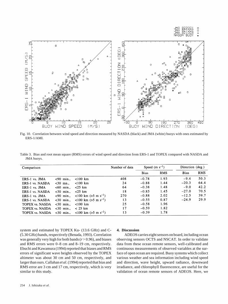
Wind speed and direction taken by NASDA and JMAbuoy were compared with ERS-1/AMI scatterometer data(Table 3). Scatterometer data observed in the innermost

three cells in the swath were excluded from the comparison,because it has been reported that the wind direction ob-served by the ERS-1 scatterometer is not accurate at lowincidence angles (Quilfen and Bentamy, 1994). All the datawith time lags <90 min. and distances <100 km are shown inFig. 10, and data of the JMA taken during two years fromJanuary 1, 1992, to December 31, 1993, were included.Generally ERS-1 data correlated well with NASDA andJMA buoy data, and no significant differences between therelationships of ERS-1 data to NASDA and JMA buoy datawere observed. The speed estimated by ERS-1 was smallerthan that of the buoys for the lower speed region, which hasbeen suggested previously (Ebuchi, 1994; Graber, 1994).Large errors in the direction estimation were also noticed,especially in the NASDA buoy data; however, the errorswere mostly for the time of low wind speed when both buoymeasurements and satellite estimation was poor.

The NASDA buoy wind speed data were also compared(Table 3) with data of TOPEX/POSEIDON (Benada, 1993).The distance between the satellite and buoy was shorter thanthat of ERS-1 because TOPEX obtains only data from nadirand because the swath coverage of the sensor was narrower.The biases of the TOPEX were smaller than ERS-1 and theRMS errors were larger. This indicates that the ERS-1algorithm may include systematic error and that TOPEXmay have random error. However, it is difficult to comparethe errors because the principle of those satellite sensors isdifferent.

Tables 4 and 5 indicate the statistics of comparisons ofsignificant wave heights measured by the NASDA buoy

Fig. 9. Correlation between SST measured by NASDA buoy anddaytime MCSST of NOAA-12/AVHRR.

Table 2. Numbers of data points taken by NASDA and JMA buoywhich coincide with observation of ERS-1 during the observa-tion of NASDA buoy. Numbers in parenthesis are numbers ofthe JMA buoys. Time lag indicates that the observation timesbetween the buoy and the satellite. Distance indicates thedistance between the buoy position and the satellite pass.

NASDA(21002)

JMA(21004) (22001)

Time lag<15 min. 8 0 0 0<30 min. 24 0 0 0<45 min. — 0 0 3<60 min. — 0 0 16<75 min. — 5 0 24<90 min. — 25 26 24

Distance<25 km 18 21 18 18<50 km 23 23 20 20<75 km 23 24 22 23

<100 km 24 25 26 24


system and estimated by TOPEX Ku- (13.6 GHz) and C-(5.30 GHz) bands, respectively (Benada, 1993). Correlationwas generally very high for both bands (r > 0.96), and biasesand RMS errors were 0–8 cm and 8–19 cm, respectively.Ebuchi and Kawamura (1994) reported that biases and RMSerrors of significant wave heights observed by the TOPEXaltimeter was about 30 cm and 50 cm, respectively, andlarger than ours. Callahan et al. (1994) reported that bias andRMS error are 3 cm and 17 cm, respectively, which is verysimilar to this study.

4. DiscussionADEOS carries eight sensors on board, including ocean

observing sensors OCTS and NSCAT. In order to validatedata from these ocean remote sensors, well-calibrated andcontinuous measurements of observed variables at the sur-face of open ocean are required. Buoy systems which collectvarious weather and sea information including wind speedand direction, wave height, upward radiance, downwardirradiance, and chlorophyll fluorescence, are useful for thevalidation of ocean remote sensors of ADEOS. Here, we

Fig. 10. Correlation between wind speed and direction measured by NASDA (black) and JMA (white) buoys with ones estimated byERS-1/AMI.

Table 3. Bias and root mean square (RMS) errors of wind speed and direction from ERS-1 and TOPEX compared with NASDA andJMA buoys.


have shown that the buoy system is useful to verify seasurface temperature, wind velocity and direction, and waveheight observed by satellite. The buoy system still requiresimprovement in the optical measurements for ocean colorremote sensing.

Validation of sea surface temperature, wind speed anddirection, and wave height observed by satellite is not new;the consistency between this study and previous studiesindicates that the NASDA buoy system is useful for theverification of those parameters. However, an increase inthe number of buoys will definitely make the satellite esti-mation of those variables more certain. A high frequency ofNASDA buoy observation will reduce the time lag betweenthe satellite and buoy data.

Table 4. Averages, standard deviations (SD), RMS errors, mean errors and correlation coefficients of wave height from TOPEX Ku-band and NASDA buoy. Units are m. WA, SA, NV stand for weighted average, simple average, and nearest value, respectively.Distance indicates the distance between the buoy location and the satellite pass.

Distance TOPEX Buoy RMS Bias Correlation Data number

Average SD Average SD

30 km WA 0.90 0.39 0.89 0.32 0.10 0.01 0.98 530 km SA 0.88 0.40 0.89 0.32 0.08 0.02 1.00 530 km NV 0.87 0.39 0.89 0.32 0.08 0.02 0.99 550 km WA 1.18 0.71 1.23 0.79 0.17 0.05 0.98 1150 km SA 1.17 0.70 1.23 0.79 0.16 0.06 0.99 1150 km NV 1.15 0.71 1.23 0.69 0.19 0.08 0.98 11


Table 5. Same as Table 4, except (TOPEX C-band).

Distance TOPEX Buoy RMS Bias Correlation Data number

Average SD Average SD



Observation of optical properties by the buoy system ismuch more difficult than other variables. For example,many spikes of chlorophyll a were seen in the raw data,mostly caused by system noise under low radiance condi-tions. The low sensitivity of the radiometer was certainly aproblem in the red light region. This is caused since theintegration times for blue and red light were same for thisexperiment. It is possible to increase the sensitivity bychanging the integration times for 400–600 nm and 600–800nm regions of these radiometers; thus the sensitivity to redlight will be increased in the next experiment.

Another problem was that three of the five cleanersystems failed during the three-month experiment. Thereasons for the problem with the cleaner system are not


known; however, one of the causes may be that the fivecleaner systems operated in the same time for this experi-ment. The simultaneous operation of the cleaner systemsmight have resulted in a lack of power. The operation timeof the cleaner system will be changed to sequential, ratherthan simultaneous, for the next experiment.

Furthermore, during this experiment, the water samplesfor chlorophyll a measurements could be taken only whenthe buoy was deployed and recovered. Also, we could notmake underwater optical measurements from the ship, co-incidental with the buoy measurements. Thus, verificationof optical signals taken by the buoy system was not sufficientduring this experiment. Subsequent experiments will requireplanning of more intensive verification of the optical systemof the buoy itself. However, the similar behavior of chlo-rophyll a concentration from the radiometer and chlorophyllfluorescence from the fluorometer indicates that the generalpattern of chlorophyll a is probably correct. Agreements ofthe explanations with simple calculations of nutrient inputinto the mixed layer and of the critical depth to the increaseand decrease of chlorophyll concentrations also indicatethat the general pattern was correct.

The results of this experiment already showed that thebuoy system will be useful for verification of wind speedand direction measured by NSCAT and sea surface tem-perature of OCTS. The ocean color part of the system is stillunderdeveloped, but the experiment made clear that severalpoints have to be improved. The buoy system was reassembledand deployed for three more months in the Suruga Bay (cf.Fig. 2) in early 1995, and more field verifications wereconducted at the time, the results being more successful(Kishino et al., 1996). The buoy system was further deployedto the the Yamato Bank located in the center of the Japan Seafrom August, 1996, for verification of ADEOS. Developmentof the optical buoy system is essential for the verification ofthe ocean satellite sensors, and the time series data obtainedby buoy system are also quite useful in understanding thetime variation of the physical and biological parameters inthe ocean.

AcknowledgementsThe TOPEX/POSEIDON altimeter data were provided

by the Physical Oceanography Distributed Active ArchiveCenter at the Jet Propulsion Laboratory. The ERS-1scatterometer data were also provided by the NASA PO-DAAC at JPL as one of the activities of the ADEOS/NSCATScience Working Team. We thank the members of theRemote Sensing Technology Center and the Japan WeatherAssociation for their help in developing and operating thebuoy. We also thank the Marine Biological Research Institutefor their technical help during the cruises, and K. Suzuki andN. Handa of Nagowa University for their pigment analysis.Special thanks are extended to the members of the ShimaneRegional Fisheries Center for providing their data. We also

thank M. Endoh, A. Harashima, H. Nagata for their helpfuldiscussion. This study was partially supported from theGlobal Environment Research Fund of the EnvironmentalAgency. The buoy system was supported by the NationalSpace Developmental Agency of Japan.

AppendixHeat flux was calculated mostly following Endoh (1992).

Total heat flux, Q, was estimated as the sum of long waveradiation, Qb, short wave radiation, Qi, latent heat, Ql, andsensible heat Qs:

Q = Qb + Qi + Ql + Qs,

Qb = 0.985σTs4(0.39 – 0.05ea

0.5)(1 – 0.6nc2),

Qi = (1 – αs)Qobs,

Ql = ClvρaCeu(qs – qa),

Qs = ρaCpCHu(Ts – Ta),

where σ (0.567 × 10–8 W m–2K–4) is the Boltzmann con-stant, Clv is the latent heat of vaporization of water (2.5 × 106

J kg–1K–1), Ce and CH are Dalton and Stanton numbers(1.3 × 10–3), and Cp is the specific heat of atmosphere(1.005 × 103 J kg–1K–1). αs is albedo of the sea surface and0.1 was used.

Atmospheric temperature (Ta), sea surface temperature(Ts), wind velocity (v), solar isolation (Qobs), atmosphericpressure (p), and relative humidity (U) were obtained by thebuoy. Saturation vapor pressure (ea), saturation specifichumidity (qs) and specific humidity (qa) can be calculated asfollows (Gill, 1982):

Log10(ew) = (0.7859 + 0.03477Ta)/(1 + 0.00412Ta),

ea = 0.98(1 + 10–6p(4.5 + 0.0006Ta2))ew,

qs = 0.62197/(p/ea – 1 + 0.62197),

qa = Uqs/(1 – qs + Uqs).

There was no data of cloud coverage, nc, from the buoy.Therefore, this was estimated from the ratio of Qobs andpredicted insolation under the clear sky, Qi0, from theSmithsonian formula (Reed, 1977):

Qi0 = A0 + A1cosφ + B1sinφ + A2cos2φ + B2sin2φ,

A0 = –15.82 + 326.87cosL,

A1 = 9.63 + 192.44cos(L + 90),


B1 = –3.27 + 108.70sinL,

A2 = –0.64 + 7.80sin2(L – 45),

B2 = –0.50 + 14.42cos2(L – 5),

φ = (t – 21) (360/365),

where L (deg) and t (days) are the latitude and date of theyear, respectively. The cloud coverage was estimated fromQobs = Qi0(1 – 0.7nc).

ReferencesBenada, R. (1993): PO.DAAC.MERGED GDR (TOPEX/

POSEIDON) USERS HANDBOOK, Rep. JPL D-8944, JetPropul. Lab., Pasadena, California, 122 pp.

Callahan, P. S., C. S. Morris and S. V. Hsiano (1994): Comparisonof TOPEX/POSEIDON σ0 and significant wave height dis-tribution to Geosat. J. Geophys. Res., 99, 25015–25024.

Dickey, T., J. Marra, T. Granata, C. Langdon, M. Hamilton, J.Wiggert, D. Siegel and A. Bratkovich (1991): Concurrent highresolution bio-optical and physical time series observations inthe Sargasso Sea during the spring of 1987. J. Geophys. Res.,96, 8643–8663.

Ebuchi, N. (1994): Validation of wind vectors observed by ADEOS-NSCAT. “NASA Scatteromter Science Working Team Meet-ing Report”, 1–3 June 1994, Kona, Hawaii, p. 144–147.

Ebuchi, N. and H. Kawamura (1994): Validation of wind speedsand significant wave height observed by the TOPEX altimeteraround Japan. J. Oceanogr., 50, 479–487.

Endoh, M. (1992): Basic observation of exchanges of energybetween atmosphere and ocean. Technical Report of Meteo-rological Research Institute, 30, 63–73 (in Japanese).

Evans, R. H. and H. R. Gordon (1994): Coastal zone color scanner“system calibration”: A retrospective examination. J. Geophys.Res., 99, 7293–7307.

Freilich, M. H. and R. S. Dunbar (1993): Derivation of satellitewind model functions using operational surface wind analy-sis: an altimeter example. J. Geophys. Res., 98, 14633–14649.

Fukuchi, M., H. Hattori, H. Sasaki and T. Hoshiai (1988): Aphytoplankton bloom and associated processes observed witha long-term moored system in Antarctic waters. Mar. Ecol.Prog. Ser., 45, 279–288.

Fukushima, H. and J. Ishizaka (1993): Special features and ap-plications of CZCS data in Asian waters. p. 213–236. In:Ocean Colour: Theory and Applications in a Decade of CZCSExperience, ed. by V. Barale and P. M. Schlittenhardt, KluwerAcademic.

Gill, A. E. (1982): Atmosphere-Ocean Dynamics. Academic Press,662 pp.

Gordon, H. R. and A. Y. Morel (1983): Remote Assessment of OceanColor for Interpretation of Satellite Visible Imagery.Springer-Verlag, 114 pp.

Gordon, H. R., D. K. Clark, J. W. Brown, O. B. Brown, R. H.Evans and W. W. Broenkow (1983): Phytoplankton pigmentconcentrations in the Middle Atlantic Bight: Comparison ofship determinations and CZCS estimates. Appl. Opt., 22, 20–36.

Graber, H. C. (1994): Intercomparison of ERS-1 scatteromterwind speeds at buoys. “NASA Scatteromter Science WorkingTeam Meeting Report”, 1–3 June 1994, Kona, Hawaii, p. 165–181.

Ichikawa, M., M. Shimanuki, K. Okada, H. Yamada, and T. Noda(1992): Development of a Buoy System for Monitoring Ma-rine Weather an Marine Life Abundance. Proceeding ofPORSEC’92, 886–891.

Ishizaka, J. (1996): Spatial and temporal variability of phyto-plankton: more than 40 years since the critical depth theory.Kaiyo Monthly, Extra Volume 10, 170–174 (in Japanese).

Ishizaka, J. and A. Harashima (1991): CZCS data number aroundJapan and surface chlorophyll data number simultaneouslyobserved by ship. Sora to Umi, 13, 1–8 (in Japanese with Englishabstract).

Ishizaka, J., H. Fukushima, M. Kishino, T. Saino and M. Takahashi(1992): Phytoplankton pigment distributions in regional up-welling around the Izu Peninsula detected by Coastal ZoneColor Scanner on May 1982. J. Oceanogr., 48, 305–327.

Japan Marine Fisheries Resources Exploitation Center (1990):Report of the Research for Offshore Fishing Ground Devel-opment, Yamato Bank, Japan Sea. Japan Marine FisheriesResources Exploitation Center, Chiyoda, Tokyo, 216 pp. (inJapanese).

Japan Marine Fisheries Resources Exploitation Center (1991):Report of the Research for Offshore Fishing Ground Devel-opment, Yamato Bank, Japan Sea. Japan Marine FisheriesResources Exploitation Center, Chiyoda, Tokyo, 267 pp. (inJapanese).

Kishino, M., T. Ishimaru, K. Furuya, T. Oishi and K. Kawasaki(1995): Development of Underwater Algorithm. Institute ofPhysical and Chemical Research (Riken). Wako, Saitama, 90pp. (in Japanese).

Kishino, M., J. Ishizaka, S. Saitoh, Y. Senga and M. Utashima(1996): Verification plan of OCTS atmospheric correctionand phytoplankton pigment by moored optical buoy system. J.Geophys. Res. (submitted).

Matsumura, S., H. Masuko, H. Kawamura, M. Kishino, I. Asanuma,S. Saitoh, M. Shimamuki and M. Utashima (1992): Devel-opment of ADEOS sea-truth moored buoy system. Proceed-ings of Symposium for “Autonomous Bio-optical Ocean Ob-serving System”.

McClain, E. P., W. G. Pichel and C. C. Walton (1985): Comparativeperformance of AVHRR-based multichannel sea surfacetemperatures. J. Geophys. Res., 90, 11587–11601.

Mueller, J. L. and R. W. Austin (1995): Ocean optics protocols forSeaWiFS Validation, Revision 1. NASA Tech. Memo. 104566,Vol. 25, 67 pp.

Nishimura, S. (1983): Okhotsk Sea, Japan Sea, East China Sea. p.375–401. In: Estuaries and Enclosed Seas, ed. by B. H.Ketchum, Elsevier, Amsterdam.

NOAA/NESDIS (1991): NOAA-12 Multi-Channle Sea SurfaceTemperature Daytime Equations Regression Output,NOAA.SAT.OPS.

Obata, A., J. Ishizaka and M. Endoh (1996): Global verification ofcritical depth theory for phytoplankton bloom with climato-logical in situ temperature and satellite ocean color data. J.Geophys. Res., 101, 20657–20667.

Parsons, T. R., M. Takahashi and B. Hargrave (1984): Biological


Oceanographic Processes. 3rd edition. Pergamon Press, 330pp.

Quilfen, Y. and A. Bentamy (1994): Calibration/validation ofERS-1 scatterometer precision products. Proc. IGRASS 1994,Pasadena, 954–947.

Reed, R. K. (1977): On estimating Insolation over the ocean. J. Phys.Oceanogr., 7, 482–485.

Saitoh, S., M. Ichikawa, K. Okada and Y. Isoda (1992): Satelliteand moored buoy observations of polar frontal system over theYamato Rise in the Japan Sea. Proceeding of PORSEC’92,1016–1021.

Sakaida, F. and H. Kawamura (1992): Estimation of sea surfacetemperatures around Japan using the Advanced Very High

Resolution Radiometer (AVHRR)/NOAA-11. J. Oceanogr.,48, 179–192.

Smith, R. C. and K. S. Baker (1982): Oceanic chlorophyll concen-trations as determined by satellite (CZCS). Mar. Biol., 66, 269–279.

Smith, R. C., K. J. Walters and K. S. Baker (1991): Opticalvariability and pigment biomass in the Sargasso Sea as de-termined using deep-sea optical mooring data. J. Geophys. Res.,96, 8665–8686.

Smith, S. D. (1980): Wind stress and heat flux over the ocean ingale-force winds. J. Phys. Oceanogr. 10, 709–726.

Sverdrup, H. U. (1953): On conditions for the vernal blooming ofphytoplankton. J. Cons. Explor. Mer, 18, 287–295.

time series of physical and optical parameters off shimane

Documents