Time Series Analysis with SAS R©and RSamuel T. Croker, Independent Consultant

ABSTRACT

When you need to analyze time series data but all you have is Base SAS R©then you are faced with thedecision of how to conduct the analysis outside of SAS. This usually requires you to break the workflow intoseveral different steps, which increases both the work and potential for errors. One attractive solution is touse SAS for all data preparation and reporting while using R to conduct the analysis and data visualization.R is open source statistical computing and graphics software available for Windows, UNIX/LINUX and MacOS X. The key to the simplicity of this technique is that all of the programming can be done within a SASprogram. This technique should please both SAS and R enthusiasts and can be extended well beyond theboundaries of time series analysis.

INTRODUCTION

SAS has very powerful and useful techiniques for solving time series modeling and forecasting problems.But what do you do when you do not have a license for SAS/ETS, IML or High Performance Forecasting?R is a great alternative for conducting analysis under these conditions. “R is a language and environmentfor statistical computing and graphics.” R is open source software that is a close relative to S-Plus. Since itis open source, there are numerous “bleeding edge” techniques that are not available in SAS or any otherstatistical software. Of course you should use caution when using such techniques in analysis as applica-bility and accuracy may be suspect. You should weigh out the advantages and disadvantages carefully andconsider what the impact of an incorrect conclusion would be.

WHY USE BOTH SAS AND R?

Both SAS and R have their own advantages and disadvantages. Data manipulation is much easier in SASwhile generation of graphics can be easier in R. Also, R has many statistical features that SAS has notimplemented. Developing your own statistical routines may be easier in R than SAS, particularly if youonly have Base SAS. Although the new PROTO and FCMP procedures in SAS 9.2 may invalidate this laststatement.

The key motivation for this demonstration is the need to consider a more complex time series forecastingmodel that can be done with SAS/STAT and SAS/ETS is not available. The key disadvantage in using SASand R is that the R routines used may not have been subjected to the same level of scrutiny as the SASprocedures. This is not a trivial disadvantage and must be considered very carefully.

COMPARING SAS/ETS AND R FOR TIME SERIES ANALYSIS

INDIVIDUAL SAS AND R ELEMENTS

THE SAS PART

Data manipulation is much easier in SAS than in R. Assuming that only Base SAS is licensed, then youdo not have access to SAS/ACCESS features that allow writing to databases. So the data will need tobe written to a flat file that R can then import easily. R does not require that a time series object be timeindexed as SAS does, but this means that the time series has to be adjusted before sending it over to R.First you have to make sure that the time series is complete, meaning that it is composed of equally timespaced observations with no missing values.

One effective way to make sure that a time series is complete without using the EXPAND or TIMESERIESprocedures is to merge a complete time sequence to your data then aggregate to the level desired. Ifyou have transactional data that is dense at the hourly level but not at the minute level then it would beappropriate to aggregate to the hourly level. This can easily be done with the MEANS procedure: First,create a SAS DATESTAMP value that only goes down to the hour:

1

Paper ST-146

data have;set have;tx_datestamp=DHMS(mdy(month,day,year),hour,0,0);

run;

proc means data=have NWAY NOPRINT;class year month day hour;output out=want

sum(transaction_value)=hourly_value;run;

This will sum up all of the transaction value variables to the hour on the day, month and year thatthey occurred, but missing hourly values will not be accounted for. It may be more appropriate to take theaverage or median instead of the sum depending on the type of variable that you are aggregating.

To ensure that the time series is complete in terms of the missing hourly observations, first create a datasetthat has an hourly observation for every possible observation in the WANT dataset.

Next, calculate the minimum and maximum dates. the SELECT INTO tool in PROC SQL is handy for doingthis as shown below, but there are other methods as well. In this case the select statement will returntwo columns corresponding to the minimum and maximum dates of the series and the into : stores theresults in the macro variables startdate and enddate.

proc sql noprint;select

min(tx_datestamp),max(tx_datestamp)into

:startdate,:enddate

from WANT;quit;

Then, create the date sequence with correctly formatted missing values. All that this data step does iscreate a template data set with every expected date/time (no missing values) at the correct interval withzeros for the value. If you want to have a different default value for missing values then substitute the zerowith this value. SAS recognizes DTHOUR as an interval of one hour applied to a datetime variable. You mayremember that dates and times in SAS are represented internally by numeric values. For datetime variablesthis integer representation is the number of seconds since Jan 1, 1960. To increment by one hour you couldalso use by 3600 in place of by dthour.

data hourly_template;hourly_value=0;do &startdate to &enddate by dthour;output;end;run;

In this example a missing value is a structural zero. This means that missing = 0 and assumes that themissing values were not due to a measurement malfunction or some other error.

Finally, merge the complete hourly template to the existing hourly sums. The resulting dataset should haveall of the data from the WANT dataset with missing dates filled in with zeros.

data finalseriesmerge want (in=y1)

hourly_template (in=y2);

2

if y1;by hourly_value;run;

Again, if SAS/ETS is available then PROC TIMESERIES or PROC EXPAND will handle this problem withmuch less code.

A BRIEF INTRODUCTION OF TIME SERIES ANALYSIS WITH R

There are a few ways of integrating R into a SAS programming framework but it is perhaps best to keep it assimple as possible. The method described here will create an R program using put statements in the datastep, written out to a file. Then the R program will be called using the X command. This is the simplest wayto call R by executing the R command line via the SAS X command, which accesses the operating systemshell.

For the sake of simplicity the R functions utilized are shown in the most basic state.

Plotting the Time Series Attributes The R functions used below all act upon R time series objects. Rtime series objects do not have to have a time index and can be simply a vector of observations. It is up tothe user to ensure that they are comprised of equally spaced and complete observations. The library()function ensures that the R tseries library is loaded. This library contains a time series object called airwhich is the classic airline passenger data frequently referenced in the literature of time series analysis. Tolook at the time series itself you can use the tsplot(tsobject) function.

library(tseries)air <- AirPassengersts.plot(air)acf(air)pacf(air)

Time

air

1950 1952 1954 1956 1958 1960

100

200

300

400

500

600

0.0 0.5 1.0 1.5

−0.

20.

00.

20.

40.

60.

81.

0

Lag

AC

F

Series air

0.5 1.0 1.5

−0.

50.

00.

51.

0

Lag

Par

tial A

CF

Series air

Figure 1: Results from R ts.plot, acf and pacf Functions

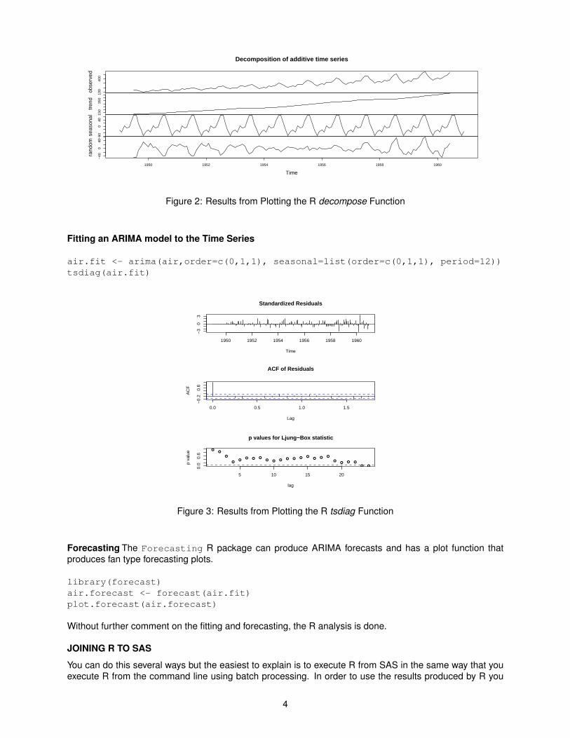
For classical additive decomposition you can use the decompose function along with the plot function.The resulting window was stretched to 900 x 300 pixels before saving.

plot(decompose(air))

Without explanation, this series looks to need a single difference and appears to have a seasonal compo-nent at a lag of 12. Tentative ARIMA fitting is done using the arima R function. The model that will be fit willbe an ARIMA(0, 1, 1) × (0, 1, 1)12. The SAS documentation has examples from many different proceduresfor analyzing this time series and can be found by searching the SAS documentation for SASHELP.AIR.There are also many different options in R for fitting time series models and only the seasonal ARIMA modeldescribed above will be covered here.

3

100

400

obse

rved

150

350

tren

d

−60

040

seas

onal

−40

040

1950 1952 1954 1956 1958 1960

rand

om

Time

Decomposition of additive time series

Figure 2: Results from Plotting the R decompose Function

Fitting an ARIMA model to the Time Series

air.fit <- arima(air,order=c(0,1,1), seasonal=list(order=c(0,1,1), period=12))tsdiag(air.fit)

Standardized Residuals

Time

1950 1952 1954 1956 1958 1960

−3

03

0.0 0.5 1.0 1.5

−0.

20.

6

Lag

AC

F

ACF of Residuals

●●

●

●●

● ● ●● ● ● ● ● ● ●

● ● ●

●● ● ●

● ●

5 10 15 20

0.0

0.6

p values for Ljung−Box statistic

lag

p va

lue

Figure 3: Results from Plotting the R tsdiag Function

Forecasting The Forecasting R package can produce ARIMA forecasts and has a plot function thatproduces fan type forecasting plots.

library(forecast)air.forecast <- forecast(air.fit)plot.forecast(air.forecast)

Without further comment on the fitting and forecasting, the R analysis is done.

JOINING R TO SAS

You can do this several ways but the easiest to explain is to execute R from SAS in the same way that youexecute R from the command line using batch processing. In order to use the results produced by R you

4

Forecasts from ARIMA(0,1,1)(0,1,1)12

1950 1952 1954 1956 1958 1960 1962

100

300

500

700

Figure 4: Results from Plotting the R plot.forecast Function

have to save the output from R in such a way that it can be used by SAS if this is desired.

Writing the R Program The initial R download also comes with a base set of packages but not all. Pack-ages are pieces of software that usually correspond to one type of analysis or research. Packages willcontain one or more libraries, which in turn contain the functions, data sets and other objects. You will seethe library R function in the code below. This function loads the ancillary library into memory but youmust first install the package from CRAN. The simplest way to do this is with the R Package Installer whichis located in the main menu under Packages or Packages and Data. This menu varies depending on whatoperating system or R version that you are using but is intuitive.

Calling the R Program

options xwait xsync;

/* three methods: *//* 1. Call R directly - Some errors are not reported to log */x "’C:\Program Files\R\R-2.6.2\bin\r.exe’

--no-save --no-restore <""&rsourcepath\source\tsdiag.r"">""&rsourcepath\output\tsdiag.out""";

/* 2. Execute via the rterm utility --errors not reported to log show in terminal*/

x c:\r\rspawn <c:\R\source\tsdiag.r> c:\R\output\tsdiag.out;/* where rspawn.bat is only:

rterm.exe --no-save --no-restoreexit

*//* 3. From data step */data _null_;

call system("rterm --no-save --no-restore<c:\R\source\tsdiag.r> c:\R\output\tsdiag.out");

run;

Returning Results to SAS

/* include the R log in the SAS log */

data _null_;infile "&rsourcepath\output\tsdiag.out";

5

file log;input;put ’R LOG: ’ _infile_;

run;

/* include the image in the sas output.Specify a file if you are not using autogenerated html output */

ods html;data _null_;

file print;put "<IMG SRC=’" "&rsourcepath\output\plot.png" "’ border=’0’>";put "<IMG SRC=’" "&rsourcepath\output\acf.png" "’ border=’0’>";put "<IMG SRC=’" "&rsourcepath\output\pacf.png" "’ border=’0’>";put "<IMG SRC=’" "&rsourcepath\output\spect.png" "’ border=’0’>";put "<IMG SRC=’" "&rsourcepath\output\fcst.png" "’ border=’0’>";

run;ods html close;

You might find the first approach the easiest to debug.

AN INTEGRATED EXAMPLE

All of the R output including source, logs and graphics will be stored in a single directory for simplicity. Inpractice it is better to put these into a file structure that makes sense for your application. For example, itmay be necessary to create sub-directories for source, output and logs.

The R source code can be written and saved separately, or it can be written out from SAS. The onlyadvantage from writing it from SAS is that all of the programming can be done from a single interface-theSAS Editor of your choice. This will be the method used here.

filename congtrez url’http://waterdata.usgs.gov/nwis/uv?cb_00065=on&format=rdb&period=31&site_no=02169810’;

data congaree_trez;infile congtrez dlm=’09’x;length agency $10 site $10 obsdatetime 8 stage 8;informat obsdatetime anydtdtm16.;format obsdatetime datetime28.

obsdate mmddyy10.;input agency @;if agency ˜= ’USGS’ then delete;input site $ obsdatetime stage;obsdate=datepart(obsdatetime);obshour=hour(obsdatetime);

run;

proc means data=congaree_treznwaynoprint;class agency site obsdate obshour;output out=congaree_trez_hourly_avg

mean(stage)=hourly_mean_stage;run;

\%let rsourcepath=c:\r_out;

6

data _null_;set congaree_trez_hourly_avg;/*write out only the hourly data

for simplicity - you can make thisas detailed as you want*/

file "&rsourcepath.\congaree_trez_hourly.dat";put hourly_mean_stage;

run;

data _null_;file "&rsourcepath.\tsdiag.r";fcst=tranwrd("&rsourcepath\fcst.png",’\’,’\\’);diag=tranwrd("&rsourcepath\plot.png",’\’,’\\’);spect=tranwrd("&rsourcepath\spect.png",’\’,’\\’);acf=tranwrd("&rsourcepath\acf.png",’\’,’\\’);pacf=tranwrd("&rsourcepath\pacf.png",’\’,’\\’);

put "library(forecast)";put "cong_trez <- read.table(’c:\\r_out\\congaree_trez_hourly.dat’)";

put ’cong_trez.ts <- ts(cong_trez)’;put ’cong_trez.fit <- arima(cong_trez.ts,order=c(1,1,0))’;/* redirect graphs to a png file */put ’png(filename="’ diag ’")’;put ’tsdiag(cong_trez.fit,6)’;put ’dev.off()’;

put ’cong_trez.fcst<-forecast.Arima(cong_trez.fit)’;

put ’png(filename="’ fcst ’")’;put ’plot.forecast(cong_trez.fcst)’;put ’dev.off()’;

put ’png(filename="’ acf ’")’;put ’acf(cong_trez.ts)’;put ’dev.off()’;

put ’png(filename="’ pacf ’")’;put ’pacf(cong_trez.ts)’;put ’dev.off()’;

put ’png(filename="’ spect ’")’;put ’spectrum(cong_trez.ts)’;put ’dev.off()’;

run;

options xwait xsync;

/* three methods: *//* 1. Call R directly - Some errors are not reported to log */x "’C:\Program Files\R\R-2.7.1\bin\r.exe’

--no-save --no-restore <""&rsourcepath\tsdiag.r"">""&rsourcepath\tsdiag.out""";

/* include the R log in the SAS log */

7

data _null_;infile "&rsourcepath\tsdiag.out";file log;input;put ’R LOG: ’ _infile_;

run;

/* include the image in the sas output.Specify a file if you are not using autogenerated html output */

ods html;data _null_;

file print;put "<IMG SRC=’" "&rsourcepath\plot.png" "’ border=’0’>";put "<IMG SRC=’" "&rsourcepath\acf.png" "’ border=’0’>";put "<IMG SRC=’" "&rsourcepath\pacf.png" "’ border=’0’>";put "<IMG SRC=’" "&rsourcepath\spect.png" "’ border=’0’>";put "<IMG SRC=’" "&rsourcepath\fcst.png" "’ border=’0’>";

run;ods html close;

CONCLUSION

Time series analysis with R from SAS is not an impossible task if you are willing to accept the method ofwriting out the R code from a SAS program, calling the code and then returning the results into SAS. Thisis very useful when working in an environment where SAS/ETS is not available and can even smooth overcolleagues who are hesitant to work with the R interface and prefer to code in SAS.

REFERENCESBox, George E.P., Gwilym M. Jenkins and Gregory C. Reinsel. 1994. Time Series Analysis:Forecasting and Control, 3rd ed. Upper Saddle River, NJ: Prentice-Hall.

Holland, Philip R. “SAS to R to SAS” PhUSE Proceedings. October 2005.<http://www.hollandnumerics.co.uk/pdf/SAS2R2SAS_paper.pdf>

Holland, Chris P., Yan Zhu “Stellar Graphs Using SAS (but not necessarily SAS/GRAPH” PharmaSUGProceedings. May 2006.<http://www.lexjansen.com/pharmasug/2006/technicaltechniques/tt17.pdf>

Shumway, Robert H. and David S. Stoffer. 2006. Time Series Analysis and Its Applications with RExamples, 2nd ed. New York: Springer Science+Business Media, LLC.

SOFTWARE RESOURCESThe R Project for Statistical Computing <http://www.R-project.org/> (Accessed March 25,2008).

R Full Reference Manual R: A Language and Environment for Statistical Computing<http://cran.r-project.org/doc/manuals/fullrefman.pdf> (Accessed March 25,2008).

R tseries Package tseries: Time series analysis and computational finance<http://cran.r-project.org/web/packages/tseries/index.html> (Accessed March25, 2008).

R forecasting Package forecasting: Bundle of forecast, fma, Mcomp, expsmooth<http://cran.r-project.org/web/packages/forecasting/index.html> (AccessedMarch 25, 2008).

8

CONTACT INFORMATION

I value and encourage your comments and questions! You can contact the author at:

Name: Samuel T. CrokerE-Mail: scoyote at scoyote.net

SAS and all other SAS Institute Inc. product or service names are registered trademarks or trademarks ofSAS Institute Inc. in the USA and other countries. R© indicates USA registration. Other brand and productnames are trademarks of their respective companies.

9