time series analysis - tanujit chakraborty's blog
TRANSCRIPT

Time Series Analysis
Samarjit Das
Economic Research Unit
Indian Statistical Institute
Kolkata-700108

2
What is Time Series?
A Time series is a set of observations, each one being
recorded at a specific time. (Annual GDP of a country, Sales
figure, etc)
A discrete time series is one in which the set of time points at
which observations are made is a discrete set. (All above
including irregularly spaced data)
Continuous time series are obtained when observations are
made continuously over some time intervals. It is a
theoretical Concept. (Roughly, ECG graph).
A discrete valued time series is one which takes discrete
values. (No of accidents, No of transaction etc.).

3
Few Time series Plots
Annual GDP of USA

4
A discrete time series is one in which the setof time points at which
observations are made is a discrete set. (All above including
irregularly spaced data)

5
Continuous time series are obtained when observations are made
continuously over some time intervals. (ECG graph).

6
A discrete valued time series is one which takes discrete values.
(No of accidents, No of transaction etc.).
Time series plot on car accident in U.K.

7
Continuous time series data (Stock returns):
-0.4
-0.3
-0.2
-0.1
0
0.1
0.2
0.3
0.4
0.5
1801
18
08
1815
18
22
1829
18
36
1843
18
50
1857
18
64
1871
18
78
1885
18
92
1899
19
06
1913
19
20
1927
19
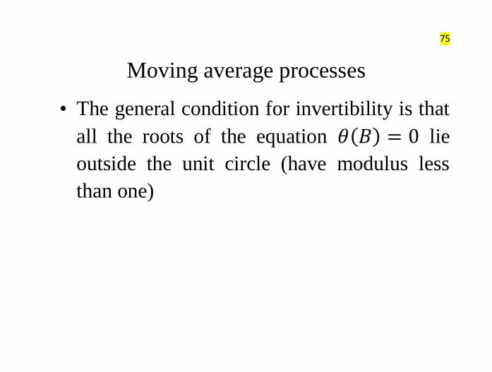
34
1941
19
48
1955
19
62
1969
19
76
1983
19
90
1997
20
04
Stock Returns
Stock Returns

8
Time series data (Number of sunspots) showing cycles:
0
50
100
150
200
250
300
350
400
1/1/
1950
1/1/
1953
1/1/
1956
1/1/
1959
1/1/
1962
1/1/
1965
1/1/
1968
1/1/
1971
1/1/
1974
1/1/
1977
1/1/
1980
1/1/
1983
1/1/
1986
1/1/
1989
1/1/
1992
1/1/
1995
1/1/
1998
1/1/
2001
1/1/
2004
1/1/
2007
1/1/
2010
Sunspots
Sunspots

9
Quarterly Sales of Ice-cream
Q1-Dec-Jan
10
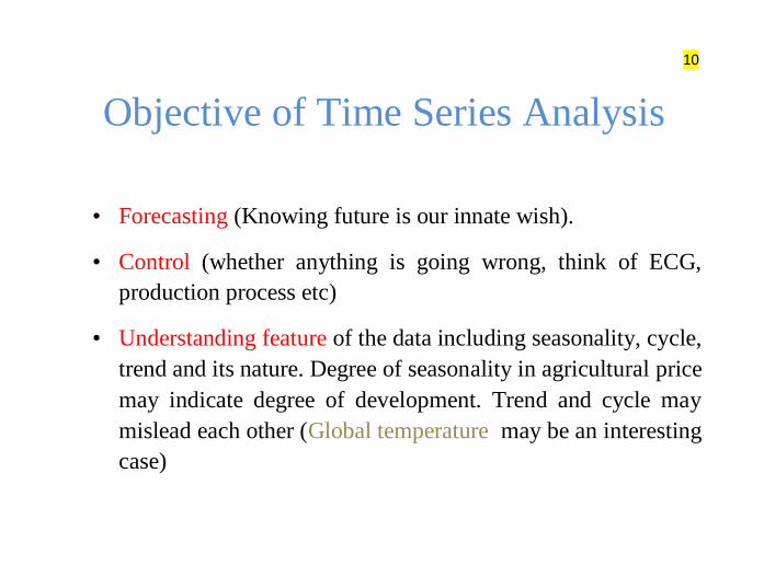
Objective of Time Series Analysis
• Forecasting (Knowing future is our innate wish).
• Control (whether anything is going wrong, think of ECG,
production process etc)
• Understanding feature of the data including seasonality, cycle,
trend and its nature. Degree of seasonality in agricultural price
may indicate degree of development. Trend and cycle may
mislead each other (Global temperature may be an interesting
case)

11
Objective
• Description: Plot the data. Try to feel the data.
Some descriptive statistics may be calculated to
get some ideas about the data.
• Explanation: Deeper understanding of the
mechanism that generated the time series.

12
Stochastic processes Approach
• Time series are an example of a stochastic or random
process
• A stochastic process is a statistical phenomenon that
evolves in time according to probabilistic laws.
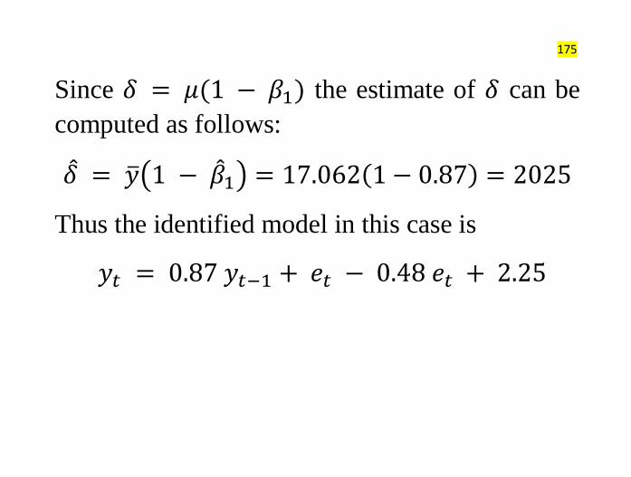
• Mathematically, a stochastic process is an indexed
collection of random variables

13
Stochastic processes
• We are concerned only with processes
indexed by time, either discrete time or
continuous time processes such as
Or

14
Stochastic Process
• A stochastic process is a collection
of random variables or a process that
develops in time according to probabilistic
laws.
• The theory of stochastic processes gives us a
formal way to look at time series variables.

15
DEFINITION
Sample Space Index Set
• For a fixed , is a random variable.
• For a given is called a sample function or a
realization as a function of

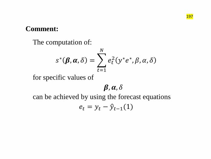
16
Stochastic Process
• Time series is a realization or sample function from a certain
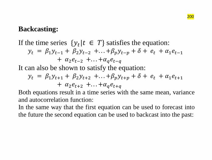
stochastic process.
• A time series is a set of observations generated sequentially in
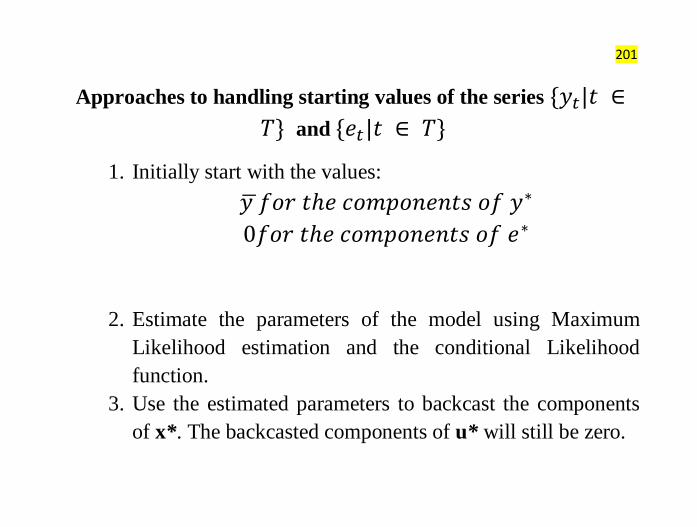
time. Therefore, they are dependent to each other. This means
that we do NOT have random sample.
• We assume that observations are equally spaced in time.
• We also assume that closer observations might have stronger
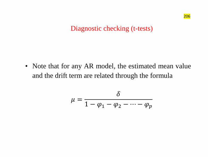
dependency.

17
JOINT PDF OF A TIME SERIES
• Remember that

18
JOINT PDF OF A TIME SERIES
• For the observed time series, say we have two
points, and .
• The marginal pdfs:
• The joint pdf:

19
JOINT PDF OF A TIME SERIES
• Since we have only one observation for each r.v.
, inference is too complicated if distributions
(or moments) change for all (i.e. change over
time). So, we need a simplification.
0
5
10
15
1 2 3 4 5 6 7 8 9 10 11 12
Y4
Y6 r.v.

20
JOINT PDF OF A TIME SERIES
• To be able to identify the structure of the series,
we need the joint pdf of However,
we have only one sample (realization). That is,
one observation from each random variable.
• This is in complete contrast to that of a cross-
section/survey data. For cross section data, for a
given population, we have a random sample.
Based on the sample we try to infer about the
population.

21
JOINT PDF OF A TIME SERIES
In Time series, each random variable has one
distribution/population. And from each
population we have just one observation. So
inference is not feasible unless we have some
strong restrictive assumptions.
• Therefore, it is very difficult to identify the joint
distribution. Hence, we need an assumption to
simplify our problem. This simplifying
assumption is known as STATIONARITY.

22
STATIONARITY
• The most vital and common assumption in time
series analysis.
• The basic idea of stationarity is that the
probability laws governing the process do not
change with time.
• The process is in statistical equilibrium.

23
Why does Stationarity Assumption work?
• Now, suppose each distribution has same mean. In that
case the common mean could be estimated based on
the realization of size ‘n’.
• We can visualize the fact in the following way---
Suppose we have 10 identical machines producing some
item, say, bulb. Suppose each machine is run for one hour.
Now it is easy to visualize that total (average) output by 10
machines is same as that of total (average) output by a
single machine running for 10 hours.
24
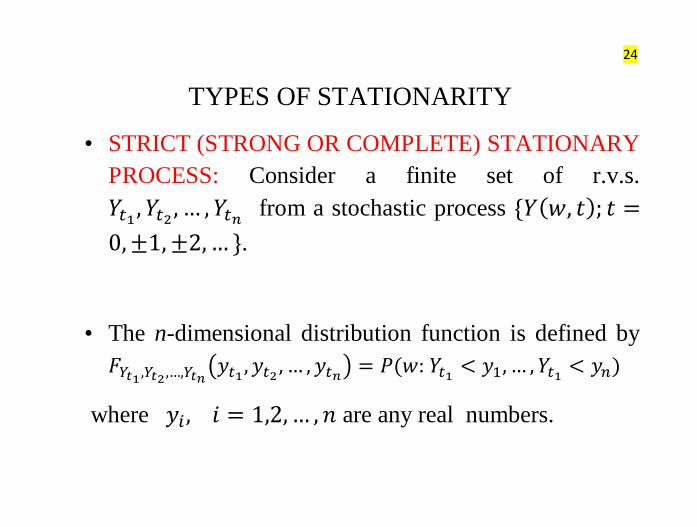
TYPES OF STATIONARITY
• STRICT (STRONG OR COMPLETE) STATIONARY
PROCESS: Consider a finite set of r.v.s.
from a stochastic process
.
• The n-dimensional distribution function is defined by
where are any real numbers.

25
STRONG STATIONARITY
• A process is said to be first order stationary in distribution,
if its one dimensional distribution function is time-invariant,
i.e.,
for any and .
• Second order stationary in distribution if
for any and .
• nth
order stationary in distribution if
for any and .

26
STRONG STATIONARITY
order stationarity in distribution = strong
stationarity
Shifting the time origin by an amount “ ” has
no effect on the joint distribution, which must
therefore depend only on time intervals between
not on absolute time, .

27
STRONG STATIONARITY
• So, for a strong stationary process
i.
ii.
Expected value of a series is constant over time, not a function of time
iii.
The variance of a series is constant over time, homoscedastic
iv.
Not constant, not depend on time, depends on time interval, which we
call “lag”, .

28
STRONG STATIONARITY
Affected from time lag, .
0
10
20
1 2 3 4 5 6 7 8 9 10 11 12

29
STRONG STATIONARITY
v.
Let and ,
Remark: We have assumed the existence of 2nd
order moments.
It is usually impossible to verify a distribution particularly a
joint distribution function from an observed time series. So,
we use weaker sense of stationarity.

30
WEAK STATIONARITY
• WEAK (COVARIANCE) STATIONARITY OR
STATIONARITY IN WIDE SENSE: A time series is
said to be covariance stationary if its first and second
order moments are unaffected by a change of time
origin.
• That is, we have constant mean and variance with
covariance and correlation beings functions of the time
difference only.

31
WEAK STATIONARITY
From, now on, when we say “stationary”, we imply weak
stationarity.

32
EXAMPLE
• Consider a time series {Yt} where
and . Is the process stationary?

33
EXAMPLE
• MOVING AVERAGE: Suppose that is
constructed as
And . Is the process stationary?

34
EXAMPLE
• RANDOM WALK
where .. Is the process stationary?

35
EXAMPLE
• Suppose that time series has the form
where and are constants and is a weakly stationary
process with mean and autocovariance function . Is
stationary?

36
EXAMPLE
where .. Is the process stationary?

37
STRONG VERSUS WEAK STATIONARITY
• Strict stationarity means that the joint distribution only depends on the
‘difference’ h, not the time (t1, . . . , tk).
• Finite variance is not assumed in the definition of strong stationarity,
therefore, strict stationarity does not necessarily imply weak
stationarity. For example, processes like i.i.d. Cauchy is strictly
stationary but not weak stationary.
• A nonlinear function of a strict stationary variable is still strictly
stationary, but this is not true for weak stationary. For example, the
square of a covariance stationary process may not have finite variance.
• Weak stationarity usually does not imply strict stationarity as higher
moments of the process may depend on time t.

38
STRONG VERSUS WEAK STATIONARITY
• If process is a Gaussian time series, which means
that the distribution functions of are all
multivariate Normal, weak stationary also implies
strict stationary. This is because a multivariate Normal
distribution is fully characterized by its first two
moments.

39
STRONG VERSUS WEAK STATIONARITY
• For example, a white noise is stationary but may not be
strict stationary, but a Gaussian white noise is strict
stationary. Also, general white noise only implies
uncorrelation while Gaussian white noise also implies
independence. Because if a process is Gaussian,
uncorrelation implies independence. Therefore, a
Gaussian white noise is just .

40
Measure of Dependence--Autocovariance
• Because the random variables comprising the process
are not independent, we must also specify their
covariance

41
Autocorrelation
• It is useful to standardize the autocovariance
function (acvf)
• Consider stationary case only
• Use the autocorrelation function (acf)

42
Autocorrelation
• More than one process can have the same acf
• Properties are:
for stationary series

43
Autocorrelation
Autocorrelation refers to the correlation of a time series with its
own past and future values.
Autocorrelation is also sometimes called “lagged correlation” or
“serial correlation”, which refers to the correlation between
members of a series of numbers arranged in time.
Positive autocorrelation might be considered a specific form of
“persistence”, a tendency for a system to remain in the same state
from one observation to the next.
For example, the likelihood of tomorrow being rainy is greater if
today is rainy than if today is dry.

44
Autocorrelations (contd.)
• A graph of the correlation values is called a
“correlogram”
• Ideally, to obtain a useful estimate of the
autocorrelation function, at least 50 observations
are needed
• Generally, The estimated autocorrelations would
be calculated up to lag no larger than N/4

45
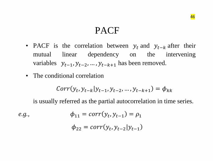
Partial Autocorrelation(PAC)
As a complementary to ACF tool, we introduce the partial autocorrelation
function, which denotes the partial correlation between and after
adjusting for . Let
where denotes linear regression of on . The quantity
are the residuals, i.e. what’s left, after linear regression using the lagged
observations.
• .
•
•
•
•
46
PACF
• PACF is the correlation between and after their
mutual linear dependency on the intervening
variables has been removed.
• The conditional correlation
is usually referred as the partial autocorrelation in time series.
e.g.,

47
CALCULATION OF PACF
1. REGRESSION APPROACH: Consider a model
from a zero mean stationary process where denotes the
coefficients of and is the zero mean error term which
is uncorrelated with
• Multiply both sides by

48
CALCULATION OF PACF
and taking the expectations
diving both sides by
Pacf

49
CALCULATION OF PACF
• For j=1,2,…,k, we have the following system of
equations
….

50
CALCULATION OF PACF
• Using Cramer’s rule successively for

51
CALCULATION OF PACF
1
1
1
1
1
1321
2311
1221
1321
2311
1221
kkk
kk
kk
kkkk
k
k
kk

52
CALCULATION OF PACF
2. Levinson and Durbin’s Recursive Formula:
Where

53
Some Popular Stochastic
Processes

54
1. White Noise:

55
White noise
• This is a purely random process, a sequence
of uncorrelated random variables
• Has constant mean and variance
• Also

56
An Illustrative plot of a white noise series

57
2. Random Walk -- A Non-stationary
Process

58
Random walk
• Start with being white noise or
purely random
• is a random walk if

59
Random walk
• The random walk is not stationary
• First differences are stationary

60
An Illustrative plot of a Random Walk

61
Some Other nonstationary series

62
Some nonstationary series (cont.)

63
Some nonstationary series (cont.)

64
3. Moving Average
Processes

65
MOVING AVERAGE PROCESSES • Suppose you win 1 Dollar if a fair coin shows a head
and lose 1 Dollar if it shows tail. Denote the outcome
on toss t by at.
• The average winning from the 4 tosses:
Moving
average process

66
MOVING AVERAGE PROCESSES • Notice that the observed series is autocorrelated
even though the generating series is uncorrelated.
• The series is the weighted aggregation of some
uncorrelated random variables.
• In Economics, the generating series, , is called the
random shock.
• Random shocks are generally unobserved and are
thought to be some unobserved economic activity.

67
MOVING AVERAGE PROCESSES
Consider a simple example:
Let be the return in stock market. Assume theta is
positive. So a good news from yesterday or a positive
activity in yesterday has a positive impact on today’s return.

68
Moving average processes • Start with being white noise or purely random,
mean zero, s.d.
• is a moving average process of order (written
MA( ) if for some constants we have
Usually

69
Moving average processes
• The mean and variance are given by
70
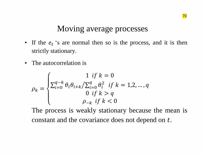
Moving average processes
• If the ‘s are normal then so is the process, and it is then
strictly stationary.
• The autocorrelation is
The process is weakly stationary because the mean is
constant and the covariance does not depend on .

71
Moving average processes
• Note the autocorrelation cuts off at lag
• For the MA(1) process with

72
Moving average processes
• In order to ensure there is a unique MA process
for a given acf, we impose the condition of
invertibility
• This ensures that when the process is written in
series form, the series converges
• For the MA(1) process , the
condition is

73
Check that
and
Both have the same autocorrelation function
The value of is same for
The 1
st one is invertible but
2nd
one is NOT.

74
Moving average processes
• For general processes introduce the backward
shift operator .
• Then the MA( ) process is given by
75
Moving average processes
• The general condition for invertibility is that
all the roots of the equation lie
outside the unit circle (have modulus less
than one)

76
MA: Stationarity
• Consider an MA(1) process without drift:
• It can be shown, regardless of the value of, that

77
MA: Stationarity
• For an MA(2) process

78
MA: Stationarity
• In general, MA processes are stationarity regardless of the
values of the parameters, but not necessarily “invertible”.
• An MA process is said to be invertible if it can be converted
into a stationary AR process of infinite order.
• In order to ensure there is a unique MA process for a given
acf, we impose the condition of invertibility.
• Therefore, invertibility condition for MA process servers two
purposes: (a) it is useful to represent an MA process as an
(infinite order) AR process; and (b) it ensures that for a given
ACF, there is an unique MA process.
79
4. Autoregressive Process

80
Autoregressive processes
• Assume is purely random with mean zero
and s.d.
• Then the autoregressive process of order or
AR( ) process is

81
Autoregressive processes
• The first order autoregression is
• Provided it may be written as an infinite
order MA process
• Using the backshift operator we have

82
Autoregressive processes
• From the previous equation we have

83
Autoregressive processes
• Then , and if

84
Autoregressive processes
• The AR(p) process can be written as

85
Autoregressive processes
• This is for
for some
This gives as an infinite MA process, so it has mean
zero

86
Autoregressive processes
• Conditions are needed to ensure that various
series converge, and hence that the variance
exists, and the autocovariance can be defined
• Essentially these are requirements that the
become small quickly enough, for large

87
Autoregressive processes
• The may not be able to be found
however.
• The alternative is to work with the
• The acf is expressible in terms of the
roots of the auxiliary
equation

88
Autoregressive processes
• Then a necessary and sufficient condition for
stationarity is that for every
• An equivalent way of expressing this is that the roots
of the equation
must lie outside the unit circle.

89
AR: Stationarity
• Suppose follows an AR(1) process without drift.
• Is stationarity?
• Note that

90
Stationarity
• Without loss of generality, assume that . Then
.
• Assuming that t is large, i.e., the process started a long
time ago, then
.1|| that provided ,)1(
)var( 12
1
2
ty It can
also be shown that provided that the same condition is
satisfied, )var()1(
)cov( 12
1
2
1t
ss
stt yyy

91
Stationarity
• Suppose the model is an AR(2) without drift,
i.e.,
• It can be shown that for yt to be stationary,
• The key point is that AR processes are not
stationary unless appropriate prior conditions
are imposed on the parameters.
tttt yyy 2211
1 || and 1 ,1 21221

92
5. Autoregressive and Moving
Average (ARMA) Processes
93
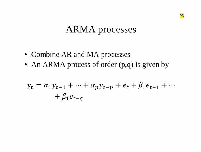
ARMA processes
• Combine AR and MA processes
• An ARMA process of order (p,q) is given by

94
ARMA processes • Alternative expressions are possible using the
backshift operator
Where

95
ARMA processes • An ARMA process can be written in pure MA or
pure AR forms, the operators being possibly of
infinite order
• Usually the mixed form requires fewer
parameters

96
6. ARIMA—Integrated ARMA

97
ARIMA processes • General autoregressive integrated moving
average processes are called ARIMA processes
• When differenced say d times, the process is an
ARMA process
• Call the differenced process . Then Wt is an
ARMA process and

98
ARIMA processes
• Alternatively specify the process as
Or
• This is an ARIMA process of order (p,d,q)

99
ARIMA processes
• The model for is non-stationary because the
AR operator on the left hand side has d roots on
the unit circle
• is often
• Random walk is ARIMA
• Can include seasonal terms

100
Non-zero mean • We have assumed that the mean is zero in the
ARIMA models
• There are two alternatives
— mean correct all the terms in the
model
— incorporate a constant term in the model
101
ACF and PACF for some
useful Models

102
Summary of the Behavior of autocorrelation and partial
autocorrelation functions
Behavior of autocorrelation and partial autocorrelation functions
Model AC PAC Autoregressive of order p
Dies down Cuts off
after lag p
Moving Average of order q
Cuts off after
lag q
Dies down
Mixed Autoregressive-Moving Average of order (p,q)
Dies down Dies down
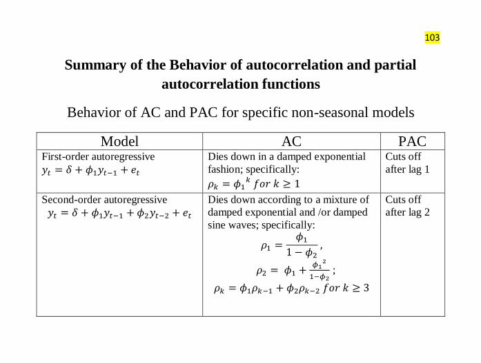
103
Summary of the Behavior of autocorrelation and partial
autocorrelation functions
Behavior of AC and PAC for specific non-seasonal models
Model AC PAC First-order autoregressive
Dies down in a damped exponential
fashion; specifically:
Cuts off
after lag 1
Second-order autoregressive
Dies down according to a mixture of
damped exponential and /or damped
sine waves; specifically:
;
Cuts off
after lag 2

104
Summary of the Behavior of autocorrelation and partial
autocorrelation functions
Behavior of AC and PAC for specific non-seasonal models
Model AC PAC First-order moving average
Cuts off after lag 1; specifically:
Dies down in a
fashion dominated
by damped
exponential decay
Second-order moving average
Cuts off after lag 2; specifically:
Dies down
according to a
mixture of damped
exponentials and
/or damped sine
waves

105
Summary of the Behavior of autocorrelation and partial
autocorrelation functions
Behavior of AC and PAC for specific non-seasonal models
Model AC PAC Mixed autoregressive-moving
average of order (1,1)
Dies down in a damped
exponential fashion;
specifically:
Dies down in a
fashion dominated
by damped
exponential decay

106
Theoretical ACs and PACs (cont.)

107
AR(1) PROCESS

108
AR(2) PROCESS
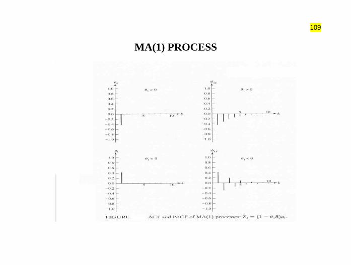
109
MA(1) PROCESS

110
MA(2) PROCESS
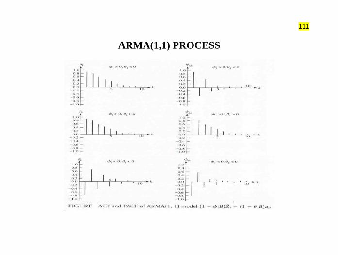
111
ARMA(1,1) PROCESS

112
ARMA(1,1) PROCESS (contd.)

113
Non-stationary
0
0.5
1
0 3 6 9 12 15 18 21 24 27 30
Stationary
0
0.5
1
0 3 6 9 12 15 18 21 24 27 30
114
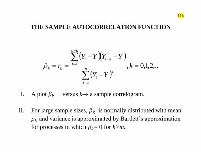
THE SAMPLE AUTOCORRELATION FUNCTION
,..2,1,0,ˆ
1
2
1
k
YY
YYYY
rn
t
t
kt
kn
t
t
kk
I. A plot versus k a sample correlogram.
II. For large sample sizes, is normally distributed with mean
and variance is approximated by Bartlett’s approximation
for processes in which = 0 for k>m.

115
THE SAMPLE AUTOCORRELATION FUNCTION
22
2
2
1 22211
ˆmk
nVar
I. In practice, i’s are unknown and replaced by their sample
estimates, . Hence, we have the following large-lag
standard error of :
22
2
2
1ˆˆ2ˆ2ˆ21
1m
ns
k
116
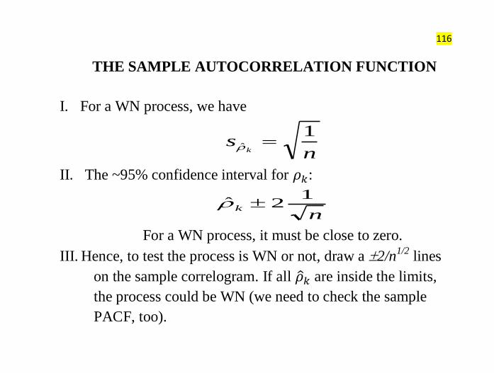
THE SAMPLE AUTOCORRELATION FUNCTION
I. For a WN process, we have
ns
k
1ˆ
II. The ~95% confidence interval for :
nk
12ˆ
For a WN process, it must be close to zero.
III. Hence, to test the process is WN or not, draw a 2/n1/2
lines
on the sample correlogram. If all are inside the limits,
the process could be WN (we need to check the sample
PACF, too).

117
THE SAMPLE PARTIAL AUTOCORRELATION
FUNCTION
.1,,2,1,ˆˆˆˆ
ˆˆ1
ˆˆˆ
ˆ
ˆˆ
,1,1
1
1
,1
1
1
,1
111
kjwhere jkkkkjkkj
k
j
jkjk
k
j
jkjkk
kk
I. For a WN process, n
Var kk
1ˆ
II. 2/n1/2
can be used as critical limits on to test the
hypothesis of a WN process.

118
Sample Partial Autocorrelation Function (SPAC)
I. may intuitively be thought of as the sample
autocorrelation of time series observations separated by a
lag k time units with the effects of the intervening
observations eliminated.
II. The standard error of is
.
III. The statistic is
.

119
Box-Jenkins Methodology
(ARIMA Models)

120
Box-Jenkins Methodology (ARIMA Models)
I. The Box-Jenkins methodology refers to a set of procedures
for identifying and estimating time series models within
the class of autoregressive integrated moving average
(ARIMA) models.
II. ARIMA models are regression models that use lagged
values of the dependent variable and/or random
disturbance term as explanatory variables.
III. ARIMA models rely heavily on the autocorrelation pattern
in the data
IV. This method applies to both non-seasonal and seasonal
data.

121
Box-Jenkins Methods--A five-step iterative
procedure
I. Stationarity Checking and Differencing
II. Model Identification
III. Parameter Estimation
IV. Diagnostic Checking
V. Forecasting

122
Step One: Stationarity checking

123
Non-Stationary
Not-stationary = Non-stationary, when
distribution (parameters) changes over time.
Various important examples are:
Deterministic trend and Stochastic trend.

124
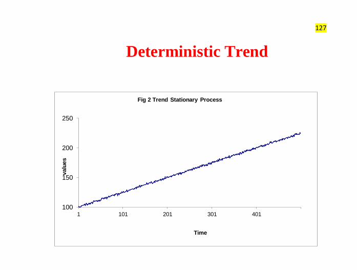
Deterministic Trend (TSP)
See that mean changes over time.
One can apply OLS to estimate the model
parameters.

125
Stochastic Trend (DSP)—Unit Root Process
This process is known as random walk.

126
Stochastic Trend
This process is known as random walk with drift.
127
Deterministic Trend
100
150
200
250
1 101 201 301 401
valu
es
Time
Fig 2 Trend Stationary Process

128
Stochastic Trend
90
100
110
120
130
1 101 201 301 401
Valu
es
Time
Figure 1: Pure Random Walk

129
Stochastic Trend
100
200
300
400
500
600
700
1 101 201 301 401
Valu
es
Time
Fig 3: Random Walk with Drift

130
Non Stationary Process
-15
-10
-5
0
5
10
15
20
1 11 21 31 41 51 61 71 81 91
Random walk with drift
stationary process
Random walk

131
TSP VS DSP
tjtj
m
j
tt eyyty
1
1 .
,
))]([(
)()(
1
0
2/12
1
0ˆ
drrW
rdWrW
t
dm
dm
Distribution (under the null of unit root) is non-standard, NOT t-
distribution or normal
This test is known as Augmented Dickey-Fuller Test (ADF).

132
Decision
I. and implies series is purely stationary.
II. and implies series is purely non-stationary,
non-stationary is due to deterministic trend.
III. and implies series is non-stationary, and
non-stationary is due to stochastic trend.

133
Differencing
I. Often non-stationary series can be made stationary through
differencing.
Examples:
stationary is7.0
but ,stationarynot is 7.07.1 )2
stationary is
but ,stationarynot is )1
11
21
1
1
ttttt
tttt
tttt
ttt
ewyyw
eyyy
eyyw
eyy

134
Differencing I. Differencing continues until stationarity is achieved.
The differenced series has n-1 values after taking the first-
difference, n-2 values after taking the second difference,
and so on.
II. The number of times that the original series must be
differenced in order to achieve stationarity is called the
order of integration, denoted by d.
III. In practice, it is almost never necessary to go beyond
second difference, because real data generally involve only
first or second level non-stationarity.

135
Differencing
I. Backward shift operator, B
II. B, operating on has the effect of shifting the data back
one period.
III. Two applications of B on shifts the data back two
periods.
IV. m applications of B on shifts the data back m periods.

136
Differencing
I. The backward shift operator is convenient for describing
the process of differencing.
II. In general, a dth-order difference can be written as
III. The backward shift notation is convenient because the
terms can be multiplied together to see the combined
effect.

137
I. If the process is non-stationary then first differences of the
series are computed to determine if that operation results
in a stationary series.
II. The process is continued until a stationary time series is
found.
III. This then determines the value of d.
IV. Sometimes, transformations, like log or some variance
stabilizing transformations are made before ‘Differencing.
138
Step Two: Model
Identification
139
Identification
Determination of the values of p and q.

140
To determine the value of p and q we use the graphical
properties of the autocorrelation function and the partial
autocorrelation function.
Again recall the following.
Auto-correlation function
Partial Autocorrelation function
Cuts off
Cuts off
Infinite. Tails off.
Dam ped Expone ntia ls
and/or Cosine wave s
Infinite. Tails off.
Infinite. Tails off.Infinite. Tails off.
Dom inated by dam ped
Exponentials & Cosine
waves.
Dom inated by dam ped
Exponentials & Cosine wave s
Dam ped Expone ntia ls
and/or Cosine wave safter q-p.
after p-q.
Process MA(q) AR(p) ARMA(p,q)
Properties of the ACF and PACF of MA, AR and ARMA Series

141
Summary: To determine p and q.
Use the following table.
MA(q) AR(p) ARMA(p,q)
ACF Cuts after q Tails off Tails off
PACF Tails off Cuts after p Tails off
Note: Usually p + q ≤ 4. There is no harm in over identifying the
time series. (Allowing more parameters in the model than
necessary. We can always test to determine if the extra parameters
are zero.)
142
Examples

143
2001000
16
17
18
Example A: "Uncontrolled" Concentration, Two-Hourly Readings:
Chemical Process

144
The data:
1 17.0 41 17.6 81 16.8 121 16.9 161 17.1 2 16.6 42 17.5 82 16.7 122 17.1 162 17.1 3 16.3 43 16.5 83 16.4 123 16.8 163 17.1 4 16.1 44 17.8 84 16.5 124 17.0 164 17.4 5 17.1 45 17.3 85 16.4 125 17.2 165 17.2 6 16.9 46 17.3 86 16.6 126 17.3 166 16.9 7 16.8 47 17.1 87 16.5 127 17.2 167 16.9 8 17.4 48 17.4 88 16.7 128 17.3 168 17.0 9 17.1 49 16.9 89 16.4 129 17.2 169 16.7 10 17.0 50 17.3 90 16.4 130 17.2 170 16.9 11 16.7 51 17.6 91 16.2 131 17.5 171 17.3 12 17.4 52 16.9 92 16.4 132 16.9 172 17.8 13 17.2 53 16.7 93 16.3 133 16.9 173 17.8 14 17.4 54 16.8 94 16.4 134 16.9 174 17.6 15 17.4 55 16.8 95 17.0 135 17.0 175 17.5 16 17.0 56 17.2 96 16.9 136 16.5 176 17.0 17 17.3 57 16.8 97 17.1 137 16.7 177 16.9 18 17.2 58 17.6 98 17.1 138 16.8 178 17.1 19 17.4 59 17.2 99 16.7 139 16.7 179 17.2 20 16.8 60 16.6 100 16.9 140 16.7 180 17.4 21 17.1 61 17.1 101 16.5 141 16.6 181 17.5 22 17.4 62 16.9 102 17.2 142 16.5 182 17.9 23 17.4 63 16.6 103 16.4 143 17.0 183 17.0 24 17.5 64 18.0 104 17.0 144 16.7 184 17.0 25 17.4 65 17.2 105 17.0 145 16.7 185 17.0 26 17.6 66 17.3 106 16.7 146 16.9 186 17.2 27 17.4 67 17.0 107 16.2 147 17.4 187 17.3 28 17.3 68 16.9 108 16.6 148 17.1 188 17.4 29 17.0 69 17.3 109 16.9 149 17.0 189 17.4 30 17.8 70 16.8 110 16.5 150 16.8 190 17.0 31 17.5 71 17.3 111 16.6 151 17.2 191 18.0 32 18.1 72 17.4 112 16.6 152 17.2 192 18.2 33 17.5 73 17.7 113 17.0 153 17.4 193 17.6 34 17.4 74 16.8 114 17.1 154 17.2 194 17.8 35 17.4 75 16.9 115 17.1 155 16.9 195 17.7 36 17.1 76 17.0 116 16.7 156 16.8 196 17.2 37 17.6 77 16.9 117 16.8 157 17.0 197 17.4 38 17.7 78 17.0 118 16.3 158 17.4 39 17.4 79 16.6 119 16.6 159 17.2 40 17.8 80 16.7 120 16.8 160 17.2

145
18 9018 6018 3018 0017 70
0
10 0
20 0
Example B: Annual Sunspot Numbers
(179 0-186 9)

146
The
Data:
Example B: Sunspot Numbers: Yearly
1770 101 1795 21 1820 16 1845 40 1771 82 1796 16 1821 7 1846 64 1772 66 1797 6 1822 4 1847 98 1773 35 1798 4 1823 2 1848 124 1774 31 1799 7 1824 8 1849 96 1775 7 1800 14 1825 17 1850 66 1776 20 1801 34 1826 36 1851 64 1777 92 1802 45 1827 50 1852 54 1778 154 1803 43 1828 62 1853 39 1779 125 1804 48 1829 67 1854 21 1780 85 1805 42 1830 71 1855 7 1781 68 1806 28 1831 48 1856 4 1782 38 1807 10 1832 28 1857 23 1783 23 1808 8 1833 8 1858 55 1784 10 1809 2 1834 13 1859 94 1785 24 1810 0 1835 57 1860 96 1786 83 1811 1 1836 122 1861 77 1787 132 1812 5 1837 138 1862 59 1788 131 1813 12 1838 103 1863 44 1789 118 1814 14 1839 86 1864 47 1790 90 1815 35 1840 63 1865 30 1791 67 1816 46 1841 37 1866 16 1792 60 1817 41 1842 24 1867 7 1793 47 1818 30 1843 11 1868 37 1794 41 1819 24 1844 15 1869 74

147
3002001000
300
400
500
600
700 Daily IBM Common Stock Closing Prices
May 17 1961-November 2 1962
Day
Price($)

148
Example C: IBM Common Stock Closing Prices: Daily (May 17 1961- Nov 2 1962)
460 471 527 580 551 523 333 394 330 457 467 540 579 551 516 330 393 340 452 473 542 584 552 511 336 409 339 459 481 538 581 553 518 328 411 331 462 488 541 581 557 517 316 409 345 459 490 541 577 557 520 320 408 352 463 489 547 577 548 519 332 393 346 479 489 553 578 547 519 320 391 352 493 485 559 580 545 519 333 388 357 490 491 557 586 545 518 344 396 492 492 557 583 539 513 339 387 498 494 560 581 539 499 350 383 499 499 571 576 535 485 351 388 497 498 571 571 537 454 350 382 496 500 569 575 535 462 345 384 490 497 575 575 536 473 350 382 489 494 580 573 537 482 359 383 478 495 584 577 543 486 375 383 487 500 585 582 548 475 379 388 491 504 590 584 546 459 376 395 487 513 599 579 547 451 382 392 482 511 603 572 548 453 370 386 487 514 599 577 549 446 365 383 482 510 596 571 553 455 367 377 479 509 585 560 553 452 372 364 478 515 587 549 552 457 373 369 479 519 585 556 551 449 363 355 477 523 581 557 550 450 371 350 479 519 583 563 553 435 369 353 475 523 592 564 554 415 376 340 479 531 592 567 551 398 387 350 476 547 596 561 551 399 387 349 478 551 596 559 545 361 376 358 479 547 595 553 547 383 385 360 477 541 598 553 547 393 385 360 476 545 598 553 537 385 380 366 475 549 595 547 539 360 373 359 473 545 595 550 538 364 382 356 474 549 592 544 533 365 377 355 474 547 588 541 525 370 376 367 474 543 582 532 513 374 379 357 465 540 576 525 510 359 386 361 466 539 578 542 521 335 387 355 467 532 589 555 521 323 386 348 471 517 585 558 521 306 389 343 Read downwards

149
Chemical Concentration data:
20 010 00
16
17
18
Example A: "Uncontro lled" Concentratio n, Two-Ho urly Rea dings:
Chemica l Pro cess
par Summary Statistics
d N Me an Std. Dev.
0 197 17.062 0.398
1 196 0.002 0.369
2 195 0.003 0.622

150
ACF and PACF for Chemical
concentration DATA
h10 20 30 40
hr
-1.0
0.0
1.0
x t
-1
0
1
10 20 30 40
kk
^
x t
k

151
ACF and PACF for Chemical
concentration DATA
-1.0
0.0
1.0hr
10 20 30 40h
x t
-1.0
0.0
1.0
kk
^x t
10 20 30 40k

152
ACF and PACF for Chemical
concentration DATA
-1.0
0.0
1.0
10 20 30 40h
x t2
hr
-1.0
0.0
1.0
10 20 30 40
kk
k
x t2
^

153
Possible Identifications
1. d = 0, p = 1, q= 1
2. d = 1, p = 0, q= 1

154
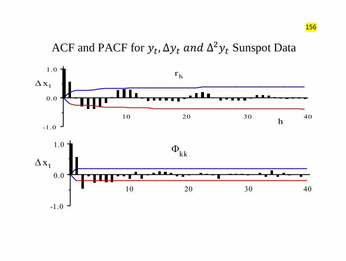
Sunspot Data:
18 9018 6018 3018 0017 70
0
10 0
20 0
Example B: Annual Sunspot Numbers
(179 0-186 9)
Summary Statistics for the Sunspot Data

155
ACF and PACF for Sunspot Data
-1.0
0.0
1.0
rh
h
10 20 30 40
x t
-1.0
0.0
1.0
x t
kk
10 20 30 40k
156
ACF and PACF for Sunspot Data
-1.0
0.0
1.0
x t
10 20 30 40h
rh
-1.0
0.0
1.0
x t
10 20 30 40
kk

157
ACF and PACF for Sunspot Data
-1.0
0.0
1.0
x t2
rh
10 20 30 40h
-1.0
0.0
1.0
10 20 30 40
kk
k
x t2

158
Possible Identification
1. d = 0, p = 2, q= 0

159
IBM stock data:
Summary Statistics
30 020 010 00
30 0
40 0
50 0
60 0
70 0 Daily IBM Commo n Stock Clo sing Prices
Ma y 17 19 61-November 2 196 2
Day
Price($)

160
ACF and PACF for (IBM Stock Price
Data)
-1.0
0.0
1.0
x t
rh
10 20 30 40h
-1.0
0.0
1.0
10 20 30 40k
kkx t

161
-1.0
0.0
1.0
rhx t
10 20 30 40h
-1.0
0.0
1.0
x t
kk
10 20 30 40k

162
-1.0
0.0
1.0rh2
x t
10 20 30 40h
-1.0
0.0
1.0
2 x t
kk
10 20 30 40k

163
Possible Identification
1. d = 1, p =0, q= 0
164
Step Three: Parameter
Estimation

165
Preliminary Estimation
Using the Method of moments
Equate sample statistics to
population parameters

166
Estimation of parameters of an MA( ) series
The theoretical autocorrelation function in terms the
parameters of an MA( ) process is given by.
To estimate , we solve the system of equations:
167
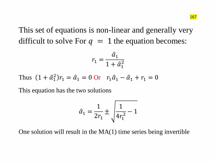
This set of equations is non-linear and generally very
difficult to solve For the equation becomes:
Thus Or
This equation has the two solutions
One solution will result in the MA(1) time series being invertible

168
For the equations become:

169
Estimation of parameters of an ARMA
series
We use a similar technique.
Namely Obtain an expression for in terms
; of and set up
equations for the estimates of ;
by replacing by .

170
Estimation of parameters of an ARMA(p,q)
series
Example: The ARMA(1,1) process
The expression for and in terms of
and are:
Further

171
Thus the expression for the estimates of
and are :
And

172
Hence
and
Or
This is a quadratic equation which can be solved

173
Example (Chemical Concentration Data)
the time series was identified as either an
ARIMA time series or an ARIMA
series.
If we use the first identification then series is
an ARMA series.

174
Identifying the series is an ARMA series.
The autocorrelation at lag is and the
autocorrelation at lag is . Thus the estimate
of is Also the quadratic equation
which has the two solutions -0.48 and -2.08. Again we
select as our estimate of to be the solution -0.48,
resulting in an invertible estimated series.
175
Since the estimate of can be
computed as follows:
Thus the identified model in this case is

176
If we use the second identification then series
– is an MA series. Thus the estimate of is:
The value of .
Thus the estimate of
is:
The estimate of , corresponds to an invertible
time series. This is the solution that we will choose.

177
The estimate of the parameter is the sample mean.
Thus the identified model in this case is:
Or
(An ARIMA model).
This compares with the other identification:
(An ARIMA model)

178
Preliminary Estimation
of the Parameters of an AR(p) Process

179
The regression coefficients and the auto
correlation function satisfy the Yule-Walker
equations:
And

180
The Yule-Walker equations can be used to estimate
the regression coefficients using the
sample auto correlation function by replacing
with .
And

181
Example
Considering the data in example 1 (Sunspot Data) the time series
was identified as an time series.
The autocorrelation at is and the autocorrelation
at is .
The equations for the estimators of the parameters of this series are
which has solution
Since then it can be estimated as follows:

182
Thus the identified model in this case is

183
Maximum Likelihood Estimation
of the parameters of an
ARMA(p,q) Series

184
The method of Maximum Likelihood Estimation
selects as estimators of a set of parameters
, the values that maximize
where is the joint
density function of the observations .
is called the Likelihood function.

185
It is important to note that:
finding the values - - to maximize
is equivalent to finding the
values to maximize
is called the log-Likelihood
function.

186
Again let be identically distributed
and uncorrelated with mean zero. In addition
assume that each is normally distributed.
Consider the time series defined by
the equation:

187
Assume that are observations on
the time series up to time .
To estimate the parameters
; , by the method
of Maximum Likelihood estimation we need to
find the joint density function of

188
We know that are independent
normal with mean zero and variance .
Thus the joint density function of is
is given by.

189
It is difficult to determine the exact density function of
from this information however if we assume
that starting values on the process
and starting values on the
process have been
observed then the conditional distribution of
given
and can easily be determined.

190
The system of equations :

191
can be solved for:
(The jacobian of the transformation is 1)

192
Then the joint density of x given and is given by:

193
Let:
= “conditional likelihood function”

194
“conditional log likelihood function” =

195
The values that maximize
and
That minimize
With

196
Comment:
The minimization of:
Requires a iterative numerical minimization procedure
to find:
• Steepest descent
• Simulated annealing
• etc
197
Comment:
The computation of:
for specific values of
can be achieved by using the forecast equations

198
Comment:
The minimization of :
assumes we know the value of starting values of the
time series and
Namely and .

199
Approaches:
1. Use estimated values
2. Use forecasting and backcasting equations to estimate
the values:
200
Backcasting:
If the time series satisfies the equation:
It can also be shown to satisfy the equation:
Both equations result in a time series with the same mean, variance
and autocorrelation function: In the same way that the first equation can be used to forecast into
the future the second equation can be used to backcast into the past:
201
Approaches to handling starting values of the series
and
1. Initially start with the values:
2. Estimate the parameters of the model using Maximum
Likelihood estimation and the conditional Likelihood
function.
3. Use the estimated parameters to backcast the components
of x*. The backcasted components of u* will still be zero.

202
4. Repeat steps 2 and 3 until the estimates stablize.
This algorithm is an application of the E-M algorithm
This general algorithm is frequently used when there are missing
values.
The E stands for Expectation (using a model to estimate the missing
values)
The M stands for Maximum Likelihood Estimation, the process
used to estimate the parameters of the model.

203
Some Examples using:
• Minitab
• Statistica
• S-Plus
• SAS

204
Step Four: Diagnostic Checking

205
Diagnostic Checking • Often it is not straightforward to determine a single
model that most adequately represents the data
generating process, and it is not uncommon to estimate
several models at the initial stage. The model that is
finally chosen is the one considered best based on a set
of diagnostic checking criteria. These criteria include
(1) t-tests for coefficient significance
(2) residual analysis
(3) model selection criteria
206
Diagnostic checking (t-tests)
• Note that for any AR model, the estimated mean value
and the drift term are related through the formula

207
Portmanteau test
• Box and Peirce proposed a statistic which
tests the magnitudes of the residual
autocorrelations as a group
• Their test was to compare below with the
Chi-Square with – – when fitting
an ARMA model

208
Portmanteau test
• Box & Ljung discovered that the test was
not good unless n was very large
• Instead use modified Box-Pierce or
Ljung-Box-Pierce statistic—reject model
if is too large

209
Residual Analysis
• If an ARMA(p,q) model is an adequate
representation of the data generating process,
then the residuals should be uncorrelated.
• Portmanteau test statistic:

210
Model Selection Criteria • Akaike Information Criterion (AIC)
• Schwartz Bayesian Criterion (SBC)
where likelihood function
number of parameters to be
estimated,
number of observations.
• Ideally, the and should be as small as
possible

211
AIC
• The Akaike Information Criterion is a
function of the maximum likelihood plus
twice the number of parameters
• The number of parameters in the formula
penalizes models with too many
parameters
212
Parsimony
• Once principal generally accepted is that models
should be parsimonious—having as few
parameters as possible
• Note that any ARMA model can be represented
as a pure AR or pure MA model, but the number
of parameters may be infinite
213
Parsimony
• AR models are easier to fit so there is a
temptation to fit a less parsimonious AR model
when a mixed ARMA model is appropriate
• Ledolter & Abraham (1981) Technometrics
show that fitting unnecessary extra parameters, or
an AR model when a MA model is appropriate,
results in loss of forecast accuracy

214
REASONS FOR USING A PARSIMONIOUS
MODEL
• Fewer numerical problems in estimation.
• Easier to understand the model.
• With fewer parameters, forecasts less sensitive to
deviations between parameters and estimates.
• Model may applied more generally to similar
processes.
• Rapid real-time computations for control or other
action.
• Having a parsimonious model is less important if the
realization is large.

215
REASONS NEEDING A LONG
REALIZATION • Estimate correlation structure (i.e., the ACF and PACF)
functions and get accurate standard errors.
• Estimate seasonal pattern (need at least 4 or 5 seasonal
periods).
• Approximate prediction intervals assume that parameters are
known (good approximation if realization is large).
• Fewer estimation problems (likelihood function better
behaved).
• Possible to check forecasts by withholding recent data .
• Can check model stability by dividing data and analyzing
both sides.

216
Step Four: Forecasting

217
FORECASTING

218
FORECASTING FROM AN ARMA MODEL
THE MINIMUM MEAN SQUARED ERROR FORECASTS
Observed time series, . n: the forecast origin

219
FORECASTING FROM AN ARMA
MODEL

220
FORECASTING FROM AN ARMA MODEL
• The stationary ARMA model for is
Or
• Assume that we have data and we want to
forecast (i.e., steps ahead from forecast origin
). Then the actual value is
221
FORECASTING FROM AN ARMA MODEL
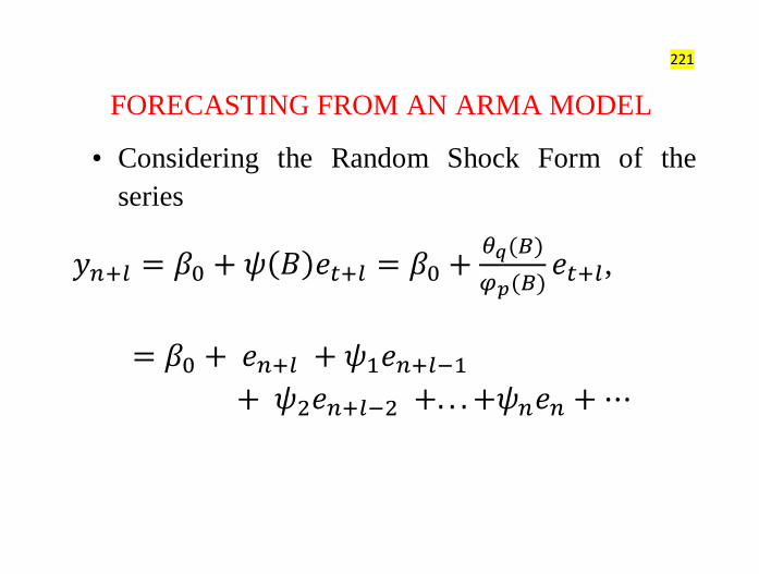
• Considering the Random Shock Form of the
series
,

222
FORECASTING FROM AN ARMA MODEL
• Taking the expectation of , we have
Where

223
FORECASTING FROM AN ARMA MODEL
The forecast error:
The expectation of the forecast error:
So, the forecast in unbiased.
The variance of the forecast error:

224
FORECASTING FROM AN ARMA MODEL
One step-ahead

225
FORECASTING FROM AN ARMA MODEL
Two step-ahead

226
FORECASTING FROM AN ARMA MODEL
Note that,
That’s why ARMA (or ARIMA) forecasting is useful
only for short-term forecasting.

227
PREDICTION INTERVAL FOR A 95% prediction interval for is
For one step-ahead this simplifies to
For one step-ahead this simplifies to

228
UPDATING THE FORECASTS
• Let’s say we have observations at time
and find a good model for this
series and obtain the forecast for ,
and so on. At , we observe
the value of Now, we want to
update our forecasts using the original
value of and the forecasted value of
it.

229
UPDATING THE FORECASTS The forecast error is
We can also write this as

230
UPDATING THE FORECASTS

231
Forecast of an AR(1) process
The forecast decays geometrically as l increases
n
l
n
nnn
nnn
nnn
nnn
nttt
ylyl
yyE
eyyl
yyE
eyyl
lyeyy
)(any for
)|(
2
)|(
1
?)(
2
2
212
1
11
1

232
Forecast of an AR(p) process
You need to calculate the previous forecasts l-1,l-2,….
)(ˆ........)2(ˆ)1(ˆ)(ˆany for
........)1(ˆ)|()2(ˆ
........2
........)|()1(ˆ
........1
?,.....),|()(ˆ
........
21
2212
222112
11211
111211
1
2211
plylylylyl
yyyyEy
eyyyyl
yyyyEy
eyyyyl
yyyEly
eyyyy
npnnn
pnpnnnnn
npnpnnn
pnpnnnnn
npnpnnn
nnlnn
tptpttt

233
Forecast of a MA(1)
That is the mean of the process
1 ttt eey
?)|()(ˆ nlnn IyEly
0)(ˆ1
02ˆ
2
)()1(ˆ
1
122
1
11
lyl
y
eeyl
eyEy
eeyl
n
n
nnn
nnn
nnn
nn yLe 1)1(

234
Forecast of a MA(q)
nq
q
n
n
lq
qlll
nlnn
t
q
qt
yBB
e
ql
qleBBBIyEly
eBBBy
....1
1 where
0
)....()|()(ˆ
)......1(
1
2
21
2
21

235
Forecast of an ARMA(1,1)
)1(ˆ....)2(ˆ)1(ˆ)(ˆ2
)()1(ˆ)2(ˆ2
1
1 re whe)1(ˆ1
)1()1(
12
11
n
l
nnn
nnnn
nnnnn
lnlnlnln
tt
ylylylyl
eyyyl
yB
Beeyyl
eeyy
eByB

236
Forecast of an ARMA(p,q)
)(ˆ....)1(ˆ)(ˆ)(ˆ....)1(ˆ)(ˆ
..........
)()(
11
1111
qleleleplylyly
eeeyyy
eByB
nqnnnpnn
qlnqlnlnplnplnln
tqtp
0)1(ˆ)(ˆ
10)(ˆ
0)(ˆ
1.....),|()(ˆ
1
1
jyeeje
jje
jyjy
jyyyEjy
jnjnjnn
n
jnn
nnjnn

237
Example: ARMA(2,2)
1211211
121!1211
22112211
ˆˆ)|()1(ˆ
1
nnnnnnn
nnnnnn
tttttt
eeyyIyEy
eeeyyyl
eeeyyy
)1(ˆˆ
)(
)(ˆ
)1(ˆ
)0(ˆ
where
211
2
2
1
nnn
nn
nn
nn
yye
yB
Be
yy
yy

238
Updating forecasts
Suppose you have information up to time n, such that
When new information comes, can we update the previous
forecasts?
)(ˆ),......2(ˆ),1(ˆ lyyy nnn
11
1
1
1
0
1
11
0 0
111
1
0
)1()(ˆ
)1(ˆ)(ˆ
)(ˆ)1(ˆ.3
)()1(
)1(.2
)(ˆ)(.1
nlnn
nlnn
nlnlnnln
nlnnl
l
j
jlnjn
l
j
l
j
jlnjjlnjn
l
j
jlnjnlnn
elyly
elyly
elyylyy
eleel
eel
elyyl

239
Problems
P1: For each of the following models:
(a) Find the l-step ahead forecast of Zn+l
(b) Find the variance of the l-step ahead forecast error for l=1, 2, and 3.
P2: Consider the IMA(1,1) model :
(a) Write down the forecast equation that generates the forecasts
(b) Find the 95% forecast limits produced by this model (c)Express the forecast as a weighted average of previous
observations.
tt
tt
tt
eyBBiii
yBBii
eyBi
)1)(-(1 )(
e )1( )(
)-(1 )(
1
2
21
1
tt eByB )1()1(

240
FORECASTS OF THE TRANSFORMED SERIES
• If you use variance stabilizing transformation, after the
forecasting, you have to convert the forecasts for the
original series.
• If you use log-transformation, you have to consider the
fact that
nnnn yyyEyyyE ln,,lnlnexp,, 11

241
FORECASTS OF THE TRANSFORMED
SERIES
If X has a normal distribution with mean and variance
2,
Hence, the minimum mean square error forecast for the
original series is given by
.2
expexp2
yE
nn ylny where
2
1ˆexp nn Vary
nn yyyE ,,1 nn yyyVar ,,1
2

242
MEASURING THE FORECAST ACCURACY

243
MEASURING THE FORECAST ACCURACY

244
MEASURING THE FORECAST ACCURACY

245
References
1. Analysis of time series, J. D. Hamilton
2. Introduction to time series analysis, Brockwell and
Davis.
3. Time series analysis, Brockwell and Davis.
4. Time Series Analysis: Forecasting and Control, Box
and Jenkins, G.C. Reinsel

246
Softwares
1. SAS
2. SPSS
3. STATA
4. Eviews
5. TSP
6. R

247
Thank You