time series analysis of gaza strip shoreline using remote sensing and...
TRANSCRIPT

Time Series Analysis of Gaza Strip Shoreline
using Remote Sensing and GIS
التحليل الزهي لشبطئ قطبع غزة ببستخدام االستشعبر عي بعد
وظن الوعلىهبث الجغرافيت
Mahmoud Shihda Adwan
Supervised by
Dr. Maher A. El-Hallaq
Assistant Professor of Surveying and Geomatics
A Thesis Submitted in Partial Fulfillment
of Requirements for the Degree of
Master in Civil Engineering.
March/2016
The Islamic University–Gaza
Research and Postgraduate Affairs
Faculty of Engineering
Master of Civil Engineering
Infrastructure
زةــغ – تــالهيــــــت اإلســـــــــبهعـالج
البحث العلوي والدراسبث العليبشئىى
الهدســـــــــــــــــــتت ــــــــــــــــــــليـك
الهدست الوديـــــــــــــتر ـــــــهبجستي
البيــــــــــــــــــــت التحتيـــــــــــــــــــت


i
DEDICATION
To the good soul of my resting father…
To my beloved mother who is the most helpful in this work…
To my wife, beautiful daughters and the sweet son for their unlimited support…
To my brothers Ahmed and Mohammed…
To those who provide me with their support to achieve this thesis successfully….
To my teachers who did all their best in helping me to finish this thesis…
To all martyrs of Palestine…
To all who loved Palestine as a home land and Islam as faith a way of life…
To all of them,
I dedicate this work.

ii
ACKNOWLEDGEMENT
First of all, I would like to express the deepest appreciation to Allah for everything that
has been given to me. I would also like to thank my mother for her continuous
encouragement.
In addition, I would like to express my gratitude to my supervisor Dr. Maher El-Hallaq
for his useful comments, remarks and engagement through the learning process of this
master thesis. Furthermore, I would like to thank my committee members, Dr.
Alaeddinne Ajamassi and Dr. Jawad El-Agha, who accept to examine this thesis.
Special thanks to Eng. Wesam Elashqar, who helped me in GIS and kindly supported
me through this thesis. Also, I wouldn’t forget Mr. Muain Abu Amsha for his help in
producing this work.
Finally, I would like to give my thanks to everybody supported me during my master
degree.
iii
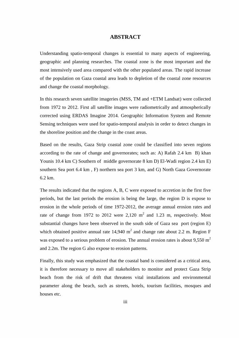
ABSTRACT
Understanding spatio-temporal changes is essential to many aspects of engineering,
geographic and planning researches. The coastal zone is the most important and the
most intensively used area compared with the other populated areas. The rapid increase
of the population on Gaza coastal area leads to depletion of the coastal zone resources
and change the coastal morphology.
In this research seven satellite imageries (MSS, TM and +ETM Landsat) were collected
from 1972 to 2012. First all satellite images were radiometrically and atmospherically
corrected using ERDAS Imagine 2014. Geographic Information System and Remote
Sensing techniques were used for spatio-temporal analysis in order to detect changes in
the shoreline position and the change in the coast areas.
Based on the results, Gaza Strip coastal zone could be classified into seven regions
according to the rate of change and governorates; such as: A) Rafah 2.4 km B) khan
Younis 10.4 km C) Southern of middle governorate 8 km D) El-Wadi region 2.4 km E)
southern Sea port 6.4 km , F) northern sea port 3 km, and G) North Gaza Governorate
6.2 km.
The results indicated that the regions A, B, C were exposed to accretion in the first five
periods, but the last periods the erosion is being the large, the region D is expose to
erosion in the whole periods of time 1972-2012, the average annual erosion rates and
rate of change from 1972 to 2012 were 2,120 m2 and 1.23 m, respectively. Most
substantial changes have been observed in the south side of Gaza sea port (region E)
which obtained positive annual rate 14,940 m2 and change rate about 2.2 m. Region F
was exposed to a serious problem of erosion. The annual erosion rates is about 9,550 m2
and 2.2m. The region G also expose to erosion patterns.
Finally, this study was emphasized that the coastal band is considered as a critical area,
it is therefore necessary to move all stakeholders to monitor and protect Gaza Strip
beach from the risk of drift that threatens vital installations and environmental
parameter along the beach, such as streets, hotels, tourism facilities, mosques and
houses etc.

iv
هلخص الدراست
إ فه ازغشاد اىبخ خالي فزشاد اض اخزفخ او ب س ازح )اضىب( ؼذ اه اجىات اهذسخ
اسبحخ ه اطمخ األوثش أهخ واسزخذاب مبسخ غ ابطك واجغشافخ واجحىس ازخططخ. إ اطمخ
اؼبخ األخشي, حش إ االصدبد اسشغ ف ازؼذاد اسىب ف اطمخ اسبحخ غضح ؤد ا اسزضاف
اصبدس اسبحخ وازغش ف شى اسبح.
ا ػب 2:83 ػب (+MSS, TM, ETM)ف هزا اجحش ر جغ سجؼخ شئبد مش اصبػ الذسبد
ERADAS Imagine, ثذاخ و اشئبد اسزخذخ ر رصححهب إشؼبػب وجىب ثبسزخذا ثشبج 3123
, ر اسزخذا ظ اؼىبد اجغشافخ ورمبد االسزشؼبس ػ ثؼذ زح اضىب وره الوزشبف 2014
زغش ف شى اسبح. ولذ ث ازح أبط ازآو واالصدبد ػ طىي ازغشاد ف ىلغ اخظ اسبح, وا
سبح لطبع غضح.
ثبء ػ زبئج اجحش ر رمس سبح لطبع غضح إ سجؼخ بطك حست ؼذالد ازغش واحبفظبد إ طمخ
9ثطىي (C)اىسط و, طمخ جىة احبفظخ 21.5ثطىي (B)و, طمخ خبىس 3.5( ثطىي Aسفح )
و, طمخ شبي بء غضح 7.5ثطىي (E)و, طمخ جىة بء غضح 3.5ثطىي (D)و, طمخ واد غضح
(F) و, وأخشا طمخ شبي غضح 4ثطىي(G) و. 7.3ثطىي
رزؼشض إ رؼبظ ف اطمخ اسبحخ وره ف افزشاد A, B, Cولذ خصذ زبئج اجحش إ أ ابطك
رزؼشض إ Dازآو أصجح هى اسبئذ, اطمخ 3123إ 3119اخس األو, و ى ف افزشح األخشح
زش. 2.34زش شثغ و 3231ثؼذي ربلص سى ػ احى ازب 3123إ 2:83رؤو ف افزشح ثؤوهب
از رزؼشض ضبدح سىخ ثؼذي (E)ش األوثش جىهشخ هى ف ابحخ اجىثخ بء اصبد ف اطمخ وازغ
رزؼشض ا حش ف اشبطئ ثشى وجش و (F)زش, ووزه اطمخ 3.3زش شثغ وؼذي رغش حىا 25:51
زش :2.5زش شثغ و 5531ثؼذي رآورزؼشض ا (G)اطمخ زش. و 3.32زش شثغ و 661:ثؼذي سى
.ف اسخ
اششظ اسبح ؼزجش طمخ حشجخ جذا زه اضشوس رحشن وبفخ اجهبد فمذ أوذد اذساسخ ثؤوأخشا
ػ طىي شالجخ وحبخ شبطئ لطبع غضح خطش االجشاف از هذد اشافك احىخ واؼب اجئخ اؼخ
اشىاسع وافبدق واالبو اسبحخ واسبجذ واجىد اخ. اشبطئ ث

v
TABLE OF CONTENTS
DEDICATION ................................................................................................................. i
ACKNOWLEDGEMENT .............................................................................................. ii
ABSTRACT .................................................................................................................... iii
الدراست هلخص ...................................................................................................................... iv
TABLE OF CONTENTS ............................................................................................... v
LIST OF TABLES ......................................................................................................... ix
LIST OF FIGURES ........................................................................................................ x
1 CHAPTER 1: INTRODUCTION .......................................................................... 1
1.1 Background ....................................................................................................... 1
1.2 Significance of Shoreline Studies ..................................................................... 1
1.3 Research Problem ............................................................................................. 1
1.4 Research Aim and Objectives ........................................................................... 2
1.5 Methodology ..................................................................................................... 2
1.6 Research Structure ............................................................................................ 3
2 CHAPTER 2: LITERATURE REVIEW ............................................................. 4
2.1 Scope ................................................................................................................. 4
2.2 Introduction ....................................................................................................... 4
2.3 Sediment Transport ........................................................................................... 4
2.3.1 Cross-shore Transport ................................................................................. 4
2.3.2 Alongshore Transport ................................................................................. 5
2.4 Definition of Shoreline ..................................................................................... 6

vi
2.5 Factors that Influence Shoreline Position Change ............................................ 6
2.6 Change Detection Definitions ........................................................................... 6
2.7 Development of Change Detection over Time ................................................. 7
2.8 Time Series Analysis Definition ....................................................................... 7
2.9 Remote Sensing ................................................................................................ 8
2.10 Shoreline Data Acquisition Techniques ........................................................... 8
2.11 Previous Coastal Studies ................................................................................... 9
2.12 Previous Studies about Gaza Strip Coast ........................................................ 16
2.13 Conclusion ...................................................................................................... 17
3 CHAPTER 3: THE STUDY AREA .................................................................... 18
3.1 Scope ............................................................................................................... 18
3.2 Historical Background .................................................................................... 18
3.3 Location and Geography ................................................................................. 18
3.4 Climate ............................................................................................................ 20
3.4.1 Air Temperature ........................................................................................ 20
3.4.2 Rainfall ...................................................................................................... 20
3.4.3 Wind Speed ............................................................................................... 21
3.4.4 Air Humidity ............................................................................................. 21
3.4.5 Solar Radiation ......................................................................................... 21
3.5 Topography ..................................................................................................... 21
3.6 Geology ........................................................................................................... 21
3.7 Gaza Beach Physical conditions ..................................................................... 22

vii
3.7.1 Geometry of the seabed (bathymetry) ...................................................... 22
3.7.2 Water Level and Tides .............................................................................. 24
3.7.3 Wind and Wave ........................................................................................ 24
3.7.4 Caostal Geology ........................................................................................ 26
3.7.5 Coast and Seabed Characteristics ............................................................. 27
3.8 Gaza Coastal Erosion ...................................................................................... 28
3.8.1 Natural Causes of Erosion ........................................................................ 28
3.8.2 Man-made Causes of Erosion ................................................................... 29
4 CHAPTER 4: METHODOLOGY ...................................................................... 31
4.1 Scope ............................................................................................................... 31
4.2 Methodology Framework ............................................................................... 31
4.3 Data Collection and Preparation ..................................................................... 33
4.3.1 Data Collection ......................................................................................... 33
4.3.2 Image Subset ............................................................................................. 34
4.3.3 Image Pre-Processing ............................................................................... 34
4.3.3.1 Geometric Correction ......................................................................... 34
4.3.3.2 Radiometric Correction ....................................................................... 34
4.3.3.3 Black Gaps Removing ........................................................................ 35
4.4 Supervised Classification ................................................................................ 37
4.5 Shoreline Extraction ....................................................................................... 39
4.6 Change Detection Analysis ............................................................................. 41
4.6.1 Area Variation ........................................................................................... 41
4.6.2 Shoreline Change Rate Computation ........................................................ 42

viii
5 CHAPTER 5: RESULTS AND DISCUSSION .................................................. 45
5.1 Scope ............................................................................................................... 45
5.2 Introduction ..................................................................................................... 45
5.3 Area Change Analysis .................................................................................... 47
5.3.1 Region A (Rafah Governorate) ................................................................. 47
5.3.2 Region B (Khan-Younis Governorate) ..................................................... 48
5.3.3 Region C (Southern of Middle Governorate) ........................................... 49
5.3.4 Region D (El-Wadi) .................................................................................. 50
5.3.5 Region E (Southern Sea Port) ................................................................... 51
5.3.6 Region F (Northern Sea Port) ................................................................... 52
5.3.7 Region G (North Governorate) ................................................................. 54
5.4 Shoreline Change Rate Analysis ..................................................................... 55
5.4.1 Region A (Rafah Governorate) ................................................................. 55
5.4.2 Region B (Khan-Younis Governorate) ..................................................... 56
5.4.3 Region C (Southern of Middle Governorate) ........................................... 57
5.4.4 Region D (El-Wadi) .................................................................................. 58
5.4.5 Region E (Southern Sea Port) ................................................................... 58
5.4.6 Region F (Northern Sea Port) ................................................................... 59
5.4.7 Region G (North of Gaza) ........................................................................ 59
6 CHAPTER 6: CONCLUSION AND RECOMMENDATIONS ....................... 63
6.1 Conclusion ...................................................................................................... 63
6.2 Recommendations ........................................................................................... 63
REFERENCES .............................................................................................................. 65
APPENDIX A: Satellite Landsat Images Subset from 1972-2012 ........................... 69
ix
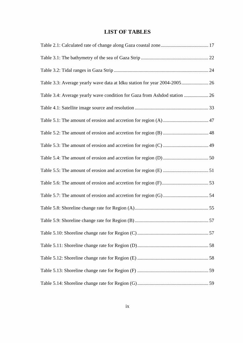
LIST OF TABLES
Table 2.1: Calculated rate of change along Gaza coastal zone ....................................... 17
Table 3.1: The bathymetry of the sea of Gaza Strip ....................................................... 22
Table 3.2: Tidal ranges in Gaza Strip ............................................................................. 24
Table 3.3: Average yearly wave data at Idku station for year 2004-2005 ...................... 26
Table 3.4: Average yearly wave condition for Gaza from Ashdod station .................... 26
Table 4.1: Satellite image source and resolution ............................................................ 33
Table 5.1: The amount of erosion and accretion for region (A) ..................................... 47
Table 5.2: The amount of erosion and accretion for region (B) ..................................... 48
Table 5.3: The amount of erosion and accretion for region (C) ..................................... 49
Table 5.4: The amount of erosion and accretion for region (D) ..................................... 50
Table 5.5: The amount of erosion and accretion for region (E) ..................................... 51
Table 5.6: The amount of erosion and accretion for region (F) ...................................... 53
Table 5.7: The amount of erosion and accretion for region (G) ..................................... 54
Table 5.8: Shoreline change rate for Region (A) ............................................................ 55
Table 5.9: Shoreline change rate for Region (B) ............................................................ 57
Table 5.10: Shoreline change rate for Region (C) .......................................................... 57
Table 5.11: Shoreline change rate for Region (D) .......................................................... 58
Table 5.12: Shoreline change rate for Region (E) .......................................................... 58
Table 5.13: Shoreline change rate for Region (F) .......................................................... 59
Table 5.14: Shoreline change rate for Region (G) .......................................................... 59

x
LIST OF FIGURES
Figure 1.1: Methodology flowchart .................................................................................. 3
Figure 2.1: a) High wave energy b) Low wave energy .................................................... 5
Figure 2.2: Longshore Current Diagram ........................................................................... 5
Figure 3.1: Gaza coastline in the Mediterranean Context .............................................. 19
Figure 3.2: Gaza Strip location ....................................................................................... 19
Figure 3.3: The average temperature of Gaza Strip between 1990-2009 ....................... 20
Figure 3.4: The bathymetric map of the sea of Gaza Strip ............................................. 23
Figure 3.5: Significant wave height vs. direction at Idku station for year 2004-2005 ... 25
Figure 3.6: Significant wave period vs. direction at Idku station for year 2004-2005 ... 25
Figure 3.7: Seabed characteristics .................................................................................. 28
Figure 3.8: Erosion problem along Beach Camp shoreline ............................................ 29
Figure 3.9: The two groins built in 1972 ........................................................................ 30
Figure 3.10: The detacher breakwaters built in 1978 ..................................................... 30
Figure 3.11: The Fishing Port built in 1994.................................................................... 30
Figure 4.1: The methodology followed in this research ................................................ 32
Figure 4.2: Noise reduction of satellite image ................................................................ 35
Figure 4.3: Black gaps removing model ......................................................................... 36
Figure 4.4: Black gap removing of satellite image ........................................................ 36
Figure 4.5: Steps for supervised classification ............................................................... 37
Figure 4.6: Supervised classification and vectorization ................................................. 38

xi
Figure 4.7: Convert polygon feature to line feature ........................................................ 39
Figure 4.8 : Extraction of shoreline ................................................................................ 39
Figure 4.9: Gaza Strip shorelines from 1972-2012 ......................................................... 40
Figure 4.10: Append two different shoreline ................................................................. 41
Figure 4.11: Change in Areas between 2002-2008 ......................................................... 41
Figure 4.12: Transect locations and change-rate using the DSAS ................................. 43
Figure 4.13: Transects cast by DSAS software .............................................................. 44
Figure 5.1: Gaza coastal zone classification ................................................................... 46
Figure 5.2: Average change rate for region A ................................................................ 48
Figure 5.3: Average change rate for region (B) .............................................................. 49
Figure 5.4: Average change rate for region (C) .............................................................. 50
Figure 5.5: Average change rate for region (D) .............................................................. 51
Figure 5.6: Average change rate for region (E) .............................................................. 52
Figure 5.7: Average change rate for region (F) .............................................................. 53
Figure 5.8: Average change rate for region (G) .............................................................. 54
Figure 5.9: Shoreline Change between 1972-2012 in region (A) ................................... 56
Figure 5.10: Annual shoreline change rate 1972-1984 ................................................... 60
Figure 5.11: Annual shoreline change rate 1984-1990 ................................................... 60
Figure 5.12: Annual shoreline change rate 1990-1998 ................................................... 60
Figure 5.13: Annual shoreline change rate 1998-2002 ................................................... 61
Figure 5.14: Annual shoreline change rate 2002-2008 ................................................... 61
Figure 5.15: Annual shoreline change rate 2008-2012 ................................................... 61

xii
LIST OF ABBREVIATIONS
AOI
Interest
Areas of Interest
AVHRR
Advanced
Very High
Resolution
Radiometer
Advanced Very High Resolution Radiometer
CTM Coastal Terrain Models
DN Digital Number
DSAS Digital Shoreline Analysis System
EPR End Point Rate
ERDAS Earth Resources Data Analysis System
ETM+
Enhanced
Thematic
Mapper Plus
Enhanced Thematic Mapper Plus
GeoTIFF Geostationary Earth Orbit Tagged Image File Format
GIS Geographic Information System
GPS Global Positioning System
HWM High Water Mark
IR Infra Red
IRS India Remote Sensing Satellite
ISODATA
Iterative Self
Iterative Self-Organizing Data Analysis Technique
LISS-III Linear Imaging Self-Scanning Sensor-III
LRR Linear Regression Rate
MODIS Moderate Resolution Imaging Spectroradiometer
MRSO Malaysian Rectified Skew Orthomorphic
MSL Mean Sea Level
MSS
Multispectral
Scanner
Multispectral Scanner
NDVI
Normalized
Difference
Vegetation
Index
Normalized Difference Vegetation Index
NOAA National Oceanic and Atmospheric Administration
NSM Net Shoreline Movement
PCA Principal Components Analysis
RS Remote Sensing
SLC-off Scan Line Corrector Failure
TM Thematic Mapper

xiii
TST Tasseled Cap Transformation
USGS U.S. Geological Survey
UTM Universal Transverse Mercator
WLR Weighted Linear Regression

1
1 CHAPTER 1: INTRODUCTION
1.1 Background
The coastal zone is the most important and the most intensively used area compared
with the other populated areas. The rapid increase of the population on and near the
coastal areas leads to an increase of coastal resources exploitation. Thus, coastal zone
areas are under great pressure from both the human activates and geomorphologic
coastal processes. In some parts along the coast of the Gaza Strip, coastal erosion is
considered a threat to buildings, roads and other installations located directly on the
coast. This is clearly seen along the coast of the city of Gaza. Erosion in the coast
occurs in the form of beach erosion. Beach erosion is the consequence of sea waves
breaking upon the coast, thereby flooding and scouring the area as it ebbs and removing
part of the unconsolidated sands. In case of higher waves, the flooding water arrives at
the Coarse sand (Kurkar) cliff removing parts of sandstone or clay beds (Abualtayef et
al., 2013).
1.2 Significance of Shoreline Studies
Change information of the earth’s surface is becoming more and more important in
monitoring the local, regional and global resources and environment. The large
collection of past and present remote sensing imagery makes it possible to analyze
spatio-temporal pattern of environmental elements and impact of human activities in
past decades (Jianya et al., 2008).
Coastal behavior must be understood in order to avoid the mistakes of the past and
ensure that the best uses will be selected for each place. Every step toward a better
understanding of the dynamics of the Gaza Strip coastal systems and forecasting its
changes with the purpose of assisting in future developments will be one more step in
the right direction.
1.3 Research Problem
The main problem is there is no studies on the Gaza strip coastal zone so the result
which obtain in this research can be used by the concerned authorities to protect the
beach from erosion. Coastal erosion is evidenced by collapsed trees, buildings, roads
and other structures, including groins which prompting the need for immediate and local
2
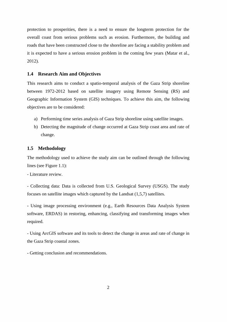
protection to prosperities, there is a need to ensure the longterm protection for the
overall coast from serious problems such as erosion. Furthermore, the building and
roads that have been constructed close to the shoreline are facing a stability problem and
it is expected to have a serious erosion problem in the coming few years (Matar et al.,
2012).
1.4 Research Aim and Objectives
This research aims to conduct a spatio-temporal analysis of the Gaza Strip shoreline
between 1972-2012 based on satellite imagery using Remote Sensing (RS) and
Geographic Information System (GIS) techniques. To achieve this aim, the following
objectives are to be considered:
a) Performing time series analysis of Gaza Strip shoreline using satellite images.
b) Detecting the magnitude of change occurred at Gaza Strip coast area and rate of
change.
1.5 Methodology
The methodology used to achieve the study aim can be outlined through the following
lines (see Figure 1.1):
- Literature review.
- Collecting data: Data is collected from U.S. Geological Survey (USGS). The study
focuses on satellite images which captured by the Landsat (1,5,7) satellites.
- Using image processing environment (e.g., Earth Resources Data Analysis System
software, ERDAS) in restoring, enhancing, classifying and transforming images when
required.
- Using ArcGIS software and its tools to detect the change in areas and rate of change in
the Gaza Strip coastal zones.
- Getting conclusion and recommendations.

3
Figure 1.1: Methodology flowchart
1.6 Research Structure
This research is oriented into six chapters;
Chapter One is intended to give a brief overview of significance of shoreline studies,
research problem, aim and objectives, general methodology as well as the structure of
this thesis.
Chapter Two gives an overview about the study area location, geography, geology,
topography, physical conditions of Gaza Strip beach such as geometry etc. Finally Gaza
coastal erosion is discussed.
In chapter Three, sediment transport, shoreline, factor that influence shoreline, change
detection and spatio-temporal analysis are defined. An overview of the change detection
methods over time is discussed. Then, case studies about coastal change detection and
Gaza shoreline are summarized from previous literatures.
In Chapter Four, methodology is described in details; image pre-processing, supervised
classification, shoreline extraction and change detection analysis are explained.
Chapter Five lists and discusses change of the Gaza Strip shoreline shape.
At the end, Chapter Six gives a general conclusion and recommendations.
Literature Review
Data Collection & Preparation
Data Extraction
Data Analysis
Conclusion &
Recommendations

4
2 CHAPTER 2: LITERATURE REVIEW
2.1 Scope
In this chapter, sediment transport, shoreline, factors that influence shoreline position
change, change detection and spatio temporal analysis (time series analysis for spatial
scenes), are defined. Then, change detection development over time, remote sensing and
shoreline data acquisition techniques are overviewed. After that, methods and case
studies about shoreline change detection are summarized from previous literatures.
Finally, previous studies about Gaza Strip shoreline are summarized from previous
literatures.
2.2 Introduction
The study of historical shoreline data can be useful to identify the predominant coastal
processes operating in specific coastal locations using change rates as an indicator of
shoreline dynamics. The real importance of such studies is to avoid decisions based on
insufficient knowledge, wrong assessments or arbitrary decisions, leading to losses in
resources and infrastructure that could have been prevented.
2.3 Sediment Transport
Sediment is any particulate matter that can be transported by fluid flow and which
eventually is deposited as a layer of solid particles on the bed or bottom of a body of
water or other liquid. Sediment, moved by waves and wind, may be academically
divided into cross-shore and alongshore sediment transport. Sediment movement can
result in erosion or accretion (removal or addition of volumes of sand). Erosion
normally results in shoreline recession (movement of the shoreline inland), accretion
causes the shoreline to move out to sea. (Matar et al., 2012)
2.3.1 Cross-shore Transport
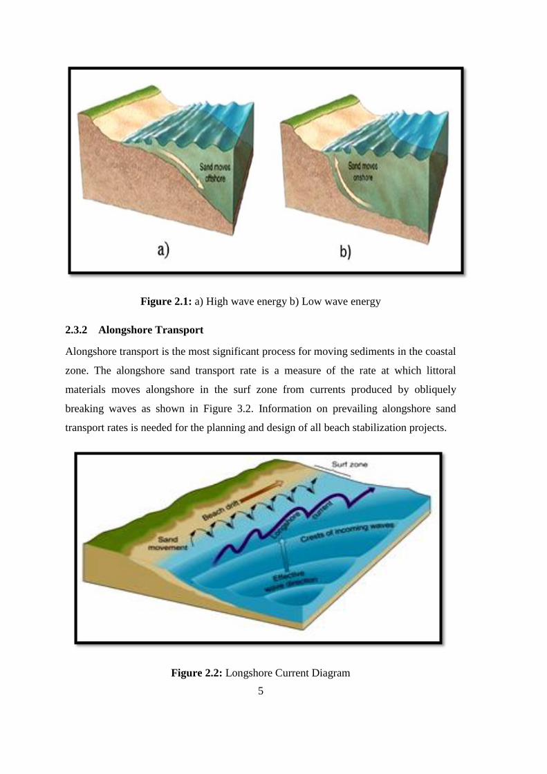
If wave energy is high the sediments carried offshore and stored as sandbar as shown in
Figure 3-1-a. And If wave energy is low the sediments carried onshore from sandbar to
buildup of sand as shown in Figure 3.1-b.
5
Figure 2.1: a) High wave energy b) Low wave energy
2.3.2 Alongshore Transport
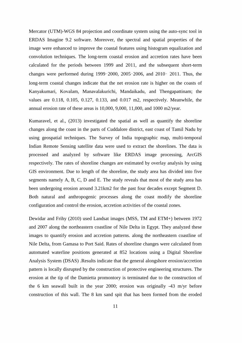
Alongshore transport is the most significant process for moving sediments in the coastal
zone. The alongshore sand transport rate is a measure of the rate at which littoral
materials moves alongshore in the surf zone from currents produced by obliquely
breaking waves as shown in Figure 3.2. Information on prevailing alongshore sand
transport rates is needed for the planning and design of all beach stabilization projects.
Figure 2.2: Longshore Current Diagram

6
2.4 Definition of Shoreline
An idealized definition of shoreline is that it coincides with the physical interface of land
and water (Dolan, et al., 1980). Despite its apparent simplicity, this definition is in practice
a challenge to apply. In reality, the shoreline position changes continually through time,
because of cross-shore and alongshore sediment movement in the littoral zone and
especially because of the dynamic nature of water levels at the coastal boundary (e.g.,
waves, tides, storm surge etc.). The shoreline must therefore be considered in a temporal
sense, and the time scale chosen will depend on the context of the investigation. For
example, the study for the purpose of investigating long-term shoreline change, sampling
every 10–20 years may be adequate. The instantaneous shoreline is the position of the land
water interface at one instant in time. As has been noted by several authors (List and Farris,
1999; Morton, 1991; Smith and Zarillo, 1990). The shoreline is a time dependent
phenomenon that may exhibit substantial short-term variability (Morton, 1991), and this
needs to be carefully considered when determining a single shoreline position. Over a
longer, engineering time scale, such as 100 years, the position of the shoreline has the
potential to vary by hundreds of meters or more (Komar, 1998).
2.5 Factors that Influence Shoreline Position Change
The transport of material along the coast is linked to natural forces such as waves, tidal
movements, long and cross-shore currents, and wind. (Anders and Byrnes, 1991)
discuss five of the primary factors that may change shoreline position: 1) wave and
current processes, 2) sea level change, 3) sediment supply, 4) coastal geology and
morphology, and 5) human intervention.
2.6 Change Detection Definitions
Singh (1989) define change detection as the process of identifying differences in the
state of an object or phenomenon by observing it at different time. Another definition of
change detection is a technology ascertaining the changes of specific features within a
certain time interval. It provides the spatial distribution of features and qualitative and
quantitative information of features changes (Kandare, 2000). Simply, U.S. Department
of Defense defines change detection as an image enhancement technique that compares
two images of the same area from different time periods. Identical picture elements are
eliminated, leaving signatures that have undergone change.

7
2.7 Development of Change Detection over Time
Change detection history starts with the history of Remote Sensing. Thereafter, the
development of change detection is closely associated with military technology during
World Wars I and II and the strategic advantage provided by temporal information
acquired by Remote Sensing. The civilian applications development of digital change
detection era really started with the launch of Landsat-1 in July 1972. However, the
development was limited by data processing technology capacities and followed closely
the development of computer technologies (Théau, 2012).
2.8 Time Series Analysis Definition
Data gathered sequentially in time are called a time series. Environmental modeling,
meteorology, hydrology, the Advanced Spaceborne Thermal Emission and Reflection
Radiometer Global Digital Elevation Model (ASTGTM-DEM) graphics and
engineering are some examples in which spatio-temporal (time series of spatial scenes)
arise. The simplest form of data used in time series is a longish series of continuous
measurements at equally spaced time points. That is, observations are made at distinct
points in time, these time points being equally spaced and, the observations may take
values from a continuous distribution. Assume that the series 𝑋𝑋𝑡𝑡runs throughout time,
that is(𝑋𝑋𝑡𝑡)𝑡𝑡=0±1±2±3…, but is only observed at times 𝑡𝑡= 1, . . . , 𝑛𝑛 (Reinert,
2010).
Time series analysis is a technology ascertaining the changes of specific features within
a certain time interval. It provides the spatial distribution of features and qualitative and
quantitative information of features changes (Kandare, 2000).
There are, obviously, numerous reasons to record and to analyze the data of a time
series. Among these is the wish to gain a better understanding of the data generating
mechanism, the prediction of future values or the optimal control of a system. The
characteristic property of a time series is the fact that the data are not generated
independently, their dispersion varies in time, they are often governed by a trend and
they have cyclic components. Statistical procedures that suppose independent and
identically distributed data are, therefore, excluded from the analysis of time series. This

8
requires proper methods that are summarized under time series analysis (Falk, et al.,
2011).
The quantitative analysis for identifying the characteristics and processes of surface
changes are carried through from the different periods of remote sensing data. It
involves the type, distribution and quantity of changes, that is the ground surface types,
boundary changes and trends before and after the changes (Shaoqing, 2008) .
Time series analysis is mainly used for temporal trajectory analysis. In contrast to bi-
temporal change detection, the temporal trajectory analysis is mostly based on low
spatial resolution images such as Advanced Very High Resolution Radiometer
(AVHRR) and Moderate Resolution Imaging Spectroradiometer (MODIS), which have
a high temporal resolution. The trade-off of using these images, however, is the lost of
spatial details that makes auto-classification very difficult, so that the temporal
trajectory analysis is commonly restricted in, for example, vegetation dynamics in large
areas, or change trajectories of individual land cover classes. Quantitative parameters
such as Normalized Difference Vegetation Index (NDVI) or area of given land cover
class are often used as the dependent variables for the establishment of change
trajectories (Jianya et al., 2008).
2.9 Remote Sensing
Over the last decade, a range of airborne, satellite, and land-based remote sensing
techniques have become more generally available to the coastal scientist, coastal
engineer, and coastal manager. Depending on the specific platform that is used, derived
shorelines may be based on the use of visually discernible coastal features, digital image
processing analysis, or a specified tidal datum.
2.10 Shoreline Data Acquisition Techniques
Various data acquisition techniques have been developed to map the position and shape
of shoreline over time (Thieler and Danforth, 1994). They include ground surveys,
aerial photography and satellite imagery.
Ground surveys maximize the contact between the researcher and the coast. They are
the most reliable technique for studying small processes in small areas. But this

9
technique requires long periods of time, can only collect a limited number of sampling
positions, and generally they provide a coarse spatial resolution.
Remote sensing technique allows for observation and measurement of coastline without
direct contact. Aerial photographs can provide two or three-dimensional measurements,
and have the advantage of covering much larger areas than ground survey method.
Aerial photographs should be considered as historical records, since they represent
objects at a given location at a precise time. But they also have some disadvantages,
since they can only be taken on daylight and through clear skies (which makes them
weather dependent), cannot properly represent objects in motion, and they require
rectification to compensate for image distortions (Ritchie et al, 1988).
Over the last three decades there has been an increasing use of satellite imagery.
Landsat and Spot and one-meter resolution Ikonos satellite images can be used to
generate relatively accurate Coastal Terrain Models (CTM) (Li, 1998). By using radar
images, data can be collected from high altitude and any time of day or night, and
atmospheric conditions are no longer a deterrent.
An automated method for shoreline extraction from raster images was developed by Liu
and Jezek (2003), who implemented a new technique based on the Canny edge detector
algorithm. This method proved to be a reliable tool to extract shoreline along extensive
coasts. Currently, the high temporal resolution and increasing spatial resolution of
remote sensing systems are available for detecting and monitoring shoreline movements
(White and El Asmar, 1999). Although remote sensing can easily delineate the shoreline
in some places, wet tidal areas still represent a problem, and conventional field-based
surveying remains as the most reliable approach to determine shoreline position change
over short time scales (Ryu et al. 2002).
2.11 Previous Coastal Studies
Mageswaran et al., (2015) study was carried out along the Nagapattinam district of
Tamil Nadu, India using multi-temporal satellite images from 1978 to 2013. The long-
term coastal erosion and accretion rates have been calculated using Digital Shoreline
Analysis System (DSAS). Linear Regression Rate (LRR) statistical method is applied to
estimate the shoreline change rate. The results of the analysis shows that erosion is

10
dominant in Sirkali, Tharangambadi, Karaikal (Puducherry State) and Nagapattinam
taluks, while Thiruthuraipundi taluk is undergoing accretion. Both natural and
anthropogenic processes along the coast control the erosion and accretion activities of
the coastal zones. The present study demonstrates that combined use of satellite imagery
and statistical methods can be a reliable method for shoreline change analysis.
Aedla et al. (2015) use an automatic shoreline detection method using histogram
equalization and adaptive thresholding techniques is developed. The shoreline of
Netravati-Gurpur river mouth area along Mangalore coast, West Coast of India have
been extracted from Indian Remote Sensing Satellite (IRS P6) LISS-III (2005, 2007 and
2010) and IRS R2 LISS-III (2013) satellite images using developed automatic shoreline
detection method. The delineated shorelines have been analyzed using Digital Shoreline
Analysis System (DSAS), a GIS Software tool for estimation of shoreline change rates
through two statistical techniques such as, End Point Rate (EPR) and Linear Regression
Rate (LRR). The Bengre spit, Northern sector of Netravati- Gurpur river mouth is
under accretion an average of 2.95 m/yr (EPR) and 3.07 m/yr (LRR) and maximum
accretion obtained is 8.51 m/yr (EPR) and 8.69 m/yr (LRR). Southern sector, the Ullal
spit is under erosion an average of -0.56 m/yr (EPR) and -0.59 m/yr (LRR).
(Alemayehu et al., 2014) find the trend of shoreline changes, and the factors attributed
to the changes. Aerial photographs of 1969 and 1989 and a recent satellite image of
2010 were used to digitize the shoreline of Watamuarea in Kenya. The Digital Shoreline
Analysis System (DSAS) in ArcGIS environment was used to create transects and
statistical analyses for the shoreline. Several Global Positioning System (GPS) points
were taken in October 2013 and 2014 during ground truthing following the High Water
Mark (HWM). The 9.8 km long Watamu shoreline was divided into 245 transects with
40 meter spacing in order to calculate the change rates. The rates of shoreline change
were calculated using the End Point Rate (EPR), Net Shoreline Movement (NSM), and
Weighted Linear Regression (WLR) statistic in DSAS.
According to Kaliraj et al (2013) , the multitemporal Landsat TM and ETM+ images
acquired from 1999 to 2011 are used as primary data source for shoreline extraction.
The Survey of India topographical maps (1:25,000) are used for preparation of the base
map. The images were geometrically corrected by applying the Universal Transverse
11
Mercator (UTM)-WGS 84 projection and coordinate system using the auto-sync tool in
ERDAS Imagine 9.2 software. Moreover, the spectral and spatial properties of the
image were enhanced to improve the coastal features using histogram equalization and
convolution techniques. The long-term coastal erosion and accretion rates have been
calculated for the periods between 1999 and 2011, and the subsequent short-term
changes were performed during 1999–2000, 2005–2006, and 2010– 2011. Thus, the
long-term coastal changes indicate that the net erosion rate is higher on the coasts of
Kanyakumari, Kovalam, Manavalakurichi, Mandaikadu, and Thengapattinam; the
values are 0.118, 0.105, 0.127, 0.133, and 0.017 m2, respectively. Meanwhile, the
annual erosion rate of these areas is 10,000, 9,000, 11,000, and 1000 m2/year.
Kumaravel, et al., (2013) investigated the spatial as well as quantify the shoreline
changes along the coast in the parts of Cuddalore district, east coast of Tamil Nadu by
using geospatial techniques. The Survey of India topographic map, multi-temporal
Indian Remote Sensing satellite data were used to extract the shorelines. The data is
processed and analyzed by software like ERDAS image processing, ArcGIS
respectively. The rates of shoreline changes are estimated by overlay analysis by using
GIS environment. Due to length of the shoreline, the study area has divided into five
segments namely A, B, C, D and E. The study reveals that most of the study area has
been undergoing erosion around 3.21km2 for the past four decades except Segment D.
Both natural and anthropogenic processes along the coast modify the shoreline
configuration and control the erosion, accretion activities of the coastal zones.
Dewidar and Frihy (2010) used Landsat images (MSS, TM and ETM+) between 1972
and 2007 along the northeastern coastline of Nile Delta in Egypt. They analyzed these
images to quantify erosion and accretion patterns. along the northeastern coastline of
Nile Delta, from Gamasa to Port Said. Rates of shoreline changes were calculated from
automated waterline positions generated at 852 locations using a Digital Shoreline
Analysis System (DSAS) .Results indicate that the general alongshore erosion/accretion
pattern is locally disrupted by the construction of protective engineering structures. The
erosion at the tip of the Damietta promontory is terminated due to the construction of
the 6 km seawall built in the year 2000; erosion was originally -43 m/yr before
construction of this wall. The 8 km sand spit that has been formed from the eroded

12
zones at the promontory tip before construction of the seawall is now under erosional
processes due to deficiency of sediment supply. Further west and prior to protection of
Ras El Bar resort, erosion (-10 m/yr) is spatially replaced by a formation of salient
accretion (15 m/yr) following emplacement of the detached breakwaters between 1991
and 2002. However, local adverse erosion has been resulted in at the western end of the
breakwater system, averaging -5 m/yr. This erosion has resulted from the interruption of
the westerly longshore sediment transport by these breakwaters. The seasonal reversal
of the North-NorthEast (NNE) waves is responsible for generating of this westward-
flowing longshore current along Ras El Bar coastline.
Remote sensing and GIS techniques was used by Mousavi et al. (2007) to determine the
morphological changes of Sefidrud delta, Iran over the last three decades (1975–2005).
Landsat MSS, TM and ETM+ and IRS data for the period of 1975 to 2005 was
processed. The data were georeferenced with respect to 1:25,000 topographic maps. All
the required datasets were registered to the IRS-Pan image. The data were then imported
into GIS environment for analyzing and possible change detection. The updated features
were digitized on screen and overlaid with the previous data. The obtained results
demonstrated that the land area eroded at an average rate of 215.6 m/yr. The Caspian
Sea level raised 2.6 m from 1975–2005, affecting the coast of Sefidrud delta
promontory. It was observed that its promontory moved to eastward about 2 km as a
maximum shoreline change over the last three decades. They emphasized the use of
geospatial information for coastline change detection.
Zakariya, et al., (2006) used Landsat 5 (1996) and Landsat 7 (2002) images to detect
shoreline areas, and the Terengganu River mouth, Malaysia. Both images were
geometrically corrected and transformed and then connected to the same spatial location
and projection. The Iterative Self-Organizing Data Analysis Technique (ISODATA)
was then used to delineate the inter-tidal zone and land and water areas. Unsupervised
classification on hue, intensity and saturation imagery with ISODATA produced
different ranges of values for the different coastal features. Spatial analysis of the
changes within a GIS permitted the detection of erosion and accretion at different
scales. Between 1996 and 2002 there was more accretion than erosion in the study area.

13
Changes along the Guamare coastline, Rio Grande do Norte State, Brazil were studied
by Grigio, et al., (2005) with remote sensing and geographic information systems
techniques. Images from Landsat 5 TM and Landsat 7 ETM+ were utilized, and the
Normalized Difference Water Index (NDWI) was computed. The authors found that the
use of the NDWI index method in Band 3 produced a large enhancement in the
submerged and emerged areas, providing a better definition of water bodies and tidal
channels. The resulting NDWI image compositions for the years 1989, 1998, 2000 and
2001 provided the required delimitation of the coastline. The results indicated that in the
time period 1998–2001 the accretion and erosion processes of the coastline were more
intense when compared with those of the earlier 1989–1998 period. In 2000–2001
erosion prevailed, contributing 78.1% of the total alteration of the coastline. GIS and
remote sensing were found to be useful to evaluate evolution of the coastline.
Muslim et al. (2004) utilizes multi-temporal satellite imagery to monitor shoreline
changes from 1992 to 2009 at Seberang Takir, Terengganu, Malaysia through the use of
image processing algorithm and statistical analysis. All the imagery was geo-rectified to
the Malaysian Rectified Skew Orthomorphic (MRSO) projection and analysis was done
to detect spatially significant areas with erosion and accretion along the shoreline and
detect potential sources of the changes. The shoreline was divided into 16 sited and
shoreline changes at the sites were determined based on satellite sensor imagery.
Preliminary result show erosion occurring near to human activities Northeast of Kuala
Terengganu shoreline while southwest of Kuala Terengganu was subjected more to
accretion.
A combination of field surveys, aerial photographs, and SPOT satellite images were
used by Fromard et al. (2004) to study coastal changes along the coast of French Guiana
for the period 1951-1999. SPOT 3 images for 1991, 1993 and 1997 and a SPOT 4
image for 1999 were geometrically corrected and exported into a geographical
information systems. Synthetic digital maps were then produced by combining the data
from the various sources in the GIS. Net accretion was observed for the period 1951
1966. Between 1966 and 1991 erosion occurred, and this was then followed by an
accretion phase. The integrated approach followed by the authors allowed them to state
that the French Guiana coastline was unstable and continuously changing.

14
Siddiqui and Maajid (2004) uses Principal Component Analysis (PCA) on Landsat MSS
and TM data to evaluate coastal changes between 1973 and 1998 in Pakistan. The multi-
temporal PCA analysis results were integrated with each other in a GIS environment.
The multi-temporal Landsat data used in this study were found to be useful for
monitoring and mapping the coastal land accretion and erosion processes. The study
provided the most recent database of the coastal environment along the coastal belt of
Karachi.
Alves et al. (2003) utilizes Landsat 5 TM imagery for monitoring and evaluating coastal
morphodynamic changes along the northeast coast of Brazil. Images for 1989 and 1998
were used to identify changes in erosional and depositional states marked by changes in
coastal geometry. In analyzing the images emphasis was placed on simple contrast
stretched false colour composites which revealed good reflectance contrast between
clear and turbid water areas. The authors were successful in evaluating different
morphodynamic areas along the coast, including beaches and dune fields. Erosion was
found to be predominant over the ten-year imaging period.
Noernberg and Marone (2003) extracts shoreline positions by employing the
Normalized Difference Water Index (NDWI) algorithm along the Brazilian coast. The
combination of Landsat imagery and the NDWI enhanced the differences in pixel
resolution between land and water. Reflectance of water was maximized at the visible
end of the electromagnetic spectrum, and minimized within the near-infrared spectrum.
Soil and vegetation land cover generated the highest reflectance in the near-infrared
portion of the spectrum.
Twelve Landsat 7 ETM+ scenes from Louisiana and Delaware were acquired by Scott
et al. (2003). The scenes were then mosaicked together to form a continuous scene, and
then processed with ERDAS Imagine. The Tasseled Cap Transformation (TCT) was
then used to extract shorelines. The TCT was chosen over other methods because it was
efficient and consistent in classifying pixels. The TCT recombined spectral information
of six ETM+ bands into three principal view components. Of the three principle view
components (i.e., brightness, greenness, and wetness) the wetness component was
exploited to differentiate land from water. The results demonstrated that shoreline data
could be defined by increasing the temporal resolution of image data sources, even if

15
the spatial resolution was decreased. The claim was made that it was possible to
accurately relate extracted shoreline data to elevation values obtained from coastal tide
observation stations.
As the spatial and temporal resolutions of satellite images have significantly improved
in recent years, the applicability of the images to coastal zone monitoring has become
more promising. Scott et al. (2002) demonstrated that Landsat 7 Thematic Mapper data
could be used to accurately extract land-water boundaries. The southern Louisiana
coastline in the winter of 2000 was classified into land and open water using the
ERDAS implementation of the tasseled cap algorithm. The land-water interface was
then traced. Though the 30-m spatial resolution is comparatively low given the dynamic
nature of the coastal region, this drawback is compensated by high color resolution, the
increased temporal resolution and decreased cost. The land-water boundary derived
from this method is equivalent in accuracy of the vector shoreline published by National
Oceanic and Atmospheric Administration (NOAA).
Landsat TM imagery was used by White and El Asmar (1999) to delineate shoreline
positions along the Nile Delta, Egypt. A segmentation algorithm permitted the
identification of known pixels of open water, referred to as ―seeds‖ to determine a
common spectral reflectance class for water. The segmentation technique merged
similar neighbouring pixels into a water classification, and proceeded to expand in a
homogenous grouping in all directions until dissimilar pixels were detected. Results
from the segmentation approach demonstrated differences in land and water areas along
the Delta. Shoreline positions were then mapped.
Li et al. (1998) used GIS application to study shoreline changes along the coast in the
state of Pinnang, Malaysia. The erosion conditions were mapped and monitored by
aerial mapping techniques, as well as a coastal geographic information systems was
developed to support modernized shoreline monitoring and management. It consists of
three components, shoreline erosion monitoring, coastal engineering management and
coastal inventory. The data involved was spatial data, time series data, social and
economic data and aerial photographs. The results showed that integration of spatial and
time series data proved a successful technique to monitor and manage the coastline.
16
2.12 Previous Studies about Gaza Strip Coast
According to Abualtayef et al., (2013) change detection analysis was used to compute
the spatial and temporal change of Gaza shoreline between 1972 and 2010. The study
area is extended from Wadi Gaza, 4 km to the south of fishing harbor, to Alsodania
area, 3 km to the north of the harbor. The study findings showed that the sediment
balance of beach area tended to be negative. This observation is based on the advance of
the waterline towards the sea to the south of fishing harbor by an average 0.75 m/year
and based on the treat of the waterline towards the land to the north of fishing harbor by
an average 1.15 m/year. Gaza fishing harbor caused a serious damage to the Beach
Camp shoreline, especially after removing six detached breakwaters. The impact of
harbor construction has extended to 2.6 km to the north and less than 2.4 km to the
south of harbor.
Abualtayef, et al., (2012) utilizes MSS, TM and ETM+ Landsat images from 1972 to
2010 to detect changes of coastal area in Gaza city to provide future database in coastal
management studies. The analysis was carried out using image processing technique
(ERDAS) and Geographical Information System platform. They applied a post
classification change detection matrix using ERDAS Imagine to estimate the amount of
change between the several dates. Then digital shoreline analysis was used to calculate
the rate of change along the Gaza coastal zone. Using ERDAS and GIS tools, the area
enclosed between four intervals is counted and the computation results of erosion and
accretion rates along Gaza coastal zone. The results showed that shoreline was
advanced south of the Gaza fishing harbor and the annual beach growth rate was 15,900
m2. On the downdrift side of the harbor, the shoreline was retreating and beaches erode
at an annual rate of -14,000 m2. While the average annual accretion and erosion rates
from 1972 to 2010 were 5.3 m and 4.7 m, respectively.
Abu-Alhin & Niemeyer (2009) use a series of Landsat ETM+ images (30m resolution),
Landsat TM-5 imagery (30m), SPOT-5 panchromatic imagery (5m) for long-term
evaluation use remote sensing and geographic information systems (GIS) to monitor
and analyze the coastline dynamics during the last two decades using medium
resolution satellite images. Tasselled Cap Transformation, Band Ratio and NDVI were
used in order to automatically extract the coastline. Accuracy assessment was performed
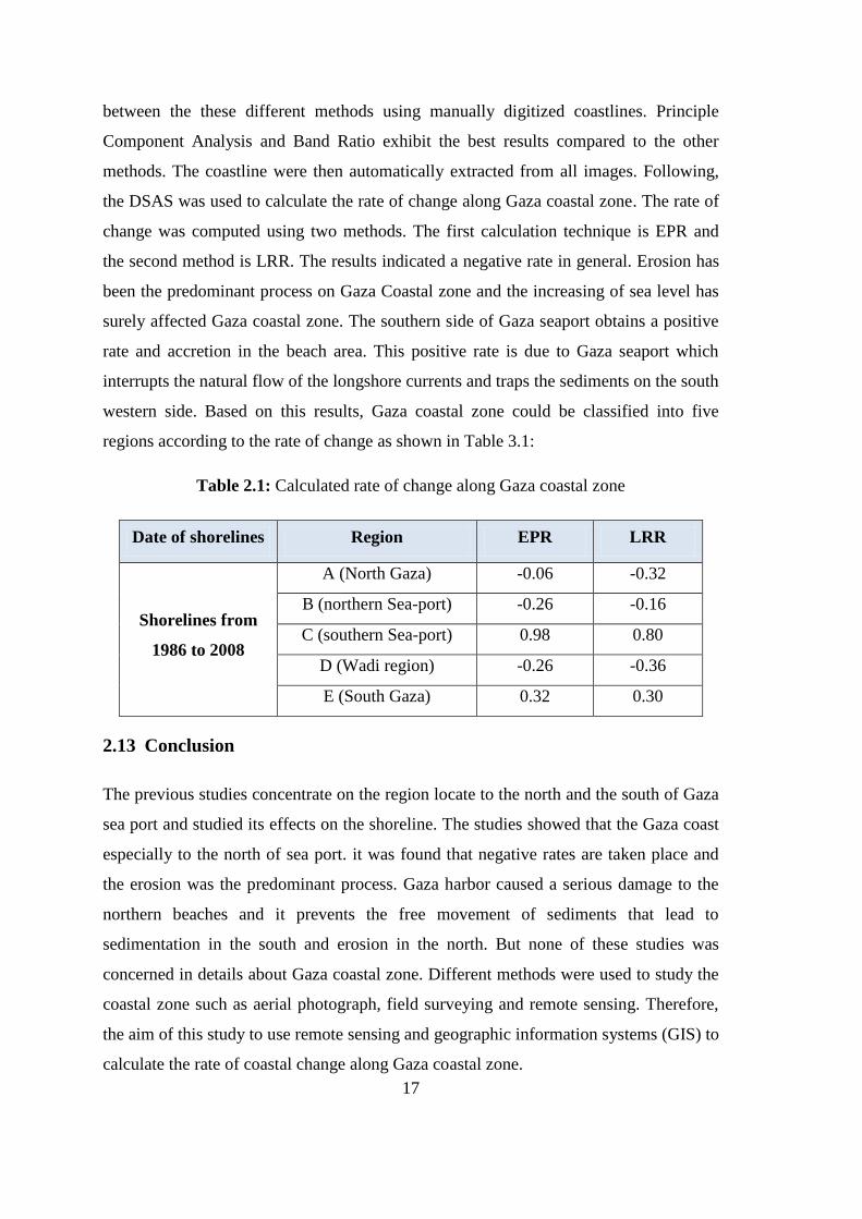
17
between the these different methods using manually digitized coastlines. Principle
Component Analysis and Band Ratio exhibit the best results compared to the other
methods. The coastline were then automatically extracted from all images. Following,
the DSAS was used to calculate the rate of change along Gaza coastal zone. The rate of
change was computed using two methods. The first calculation technique is EPR and
the second method is LRR. The results indicated a negative rate in general. Erosion has
been the predominant process on Gaza Coastal zone and the increasing of sea level has
surely affected Gaza coastal zone. The southern side of Gaza seaport obtains a positive
rate and accretion in the beach area. This positive rate is due to Gaza seaport which
interrupts the natural flow of the longshore currents and traps the sediments on the south
western side. Based on this results, Gaza coastal zone could be classified into five
regions according to the rate of change as shown in Table 3.1:
Table 2.1: Calculated rate of change along Gaza coastal zone
Date of shorelines Region EPR LRR
Shorelines from
1986 to 2008
A (North Gaza) -0.06 -0.32
B (northern Sea-port) -0.26 -0.16
C (southern Sea-port) 0.98 0.80
D (Wadi region) -0.26 -0.36
E (South Gaza) 0.32 0.30
2.13 Conclusion
The previous studies concentrate on the region locate to the north and the south of Gaza
sea port and studied its effects on the shoreline. The studies showed that the Gaza coast
especially to the north of sea port. it was found that negative rates are taken place and
the erosion was the predominant process. Gaza harbor caused a serious damage to the
northern beaches and it prevents the free movement of sediments that lead to
sedimentation in the south and erosion in the north. But none of these studies was
concerned in details about Gaza coastal zone. Different methods were used to study the
coastal zone such as aerial photograph, field surveying and remote sensing. Therefore,
the aim of this study to use remote sensing and geographic information systems (GIS) to
calculate the rate of coastal change along Gaza coastal zone.
18
3 CHAPTER 3: THE STUDY AREA
3.1 Scope
This chapter consists of eight sections. It involves location and geography which
discusses the position of the study area according to WGS84 coordinate system. Gaza
Strip climate is then reviewed temporally and quantitatively. After that, Gaza Strip
geology and topography is discussed in the fifth and sixth sections. Then Gaza beach
physical conditions such as geometry, water level, tide, wind, wave and geology of
seabed are discussed in the seventh section. Finally Gaza coastal erosion is discussed in
the eighth section.
3.2 Historical Background
The coastline of the Gaza Strip forms only a small section of a larger concave system (a
―litoral cell‖) that extends from Alexandria at the west side of the Nile Delta, via Port
Said, Bardawil Lagoon, El Arish, Gaza, ―Ashqelon‖, and ―Tel Aviv‖ to the Bay of
Haifa. This litoral cell forms the South East (SE) corner of the Levantine Basin (Figure
2.1). This entire coastline, including the coastline of the Gaza Strip, has been shaped
over the last 15,000 years by the Nile river and especially its sediment yield originating
from Africa’s mountains. The Nile sand moves along the entire concave coastline in an
anticlockwise direction, generally in a North East (NE) direction. Within this concave
SE corner of the Mediterranean, the relatively short 42 km Gaza coastline is almost
straight (Ali, 2002).
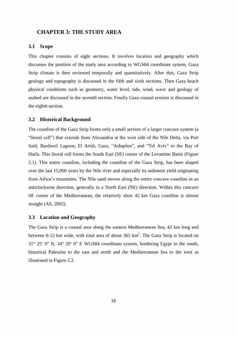
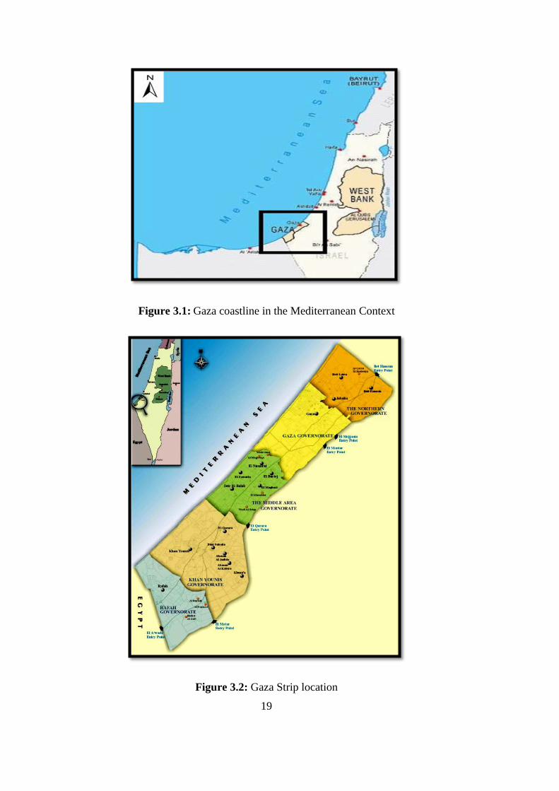
3.3 Location and Geography
The Gaza Strip is a coastal area along the eastern Mediterranean Sea, 42 km long and
between 6-12 km wide, with total area of about 365 km2. The Gaza Strip is located on
31° 25ʹ 0ʺ N, 34° 20ʹ 0ʺ E WGS84 coordinate system, bordering Egypt to the south,
historical Palestine to the east and north and the Mediterranean Sea to the west as
illustrated in Figure 2.2.
19
Figure 3.1: Gaza coastline in the Mediterranean Context
Figure 3.2: Gaza Strip location

20
3.4 Climate
3.4.1 Air Temperature
The area has a Mediterranean dry summer subtropical climate with mild winter, this is
because of its locations as transitional zone between semi-humid Mediterranean climate
and arid desert climate. The mean monthly lowest temperature in January is 15.10 C
and the highest in August is 28.30 C, with the mean annual temperature of 21.70 C (see
Figure 2.3) (3122 ,اجب).
The sea affects temperature nearby because of the moderating effect a large body of
water has on climate. During the winter, sea temperature tend to be higher than land
temperature, and vice versa during the summer months. This is the result of the water's
mass and specific heat capacity.
Figure 3.3: The average temperature of Gaza Strip between 1990-2009
3.4.2 Rainfall
The rainfall occurs in the winter period, which is between Octobers to March, and the
mean annual rainfall varies 350-400 mm per year (PNA-MEA, 2000).
0
5
10
15
20
25
30
35
Min Temp Avg Temp Max Temp
21
3.4.3 Wind Speed
The wind velocity with northwest direction at 2 meter above the surface in the summer
is about 1.5 m/s, which is less than that's during winter months where velocity reaches
values of 2.8 m/s (PNA-MEA, 2000).
3.4.4 Air Humidity
The daily relative humidity varies between 66% in the night to 86% at the daytime in
summer and between 53% to 81% respectively in winter (Matar et al., 2012).
3.4.5 Solar Radiation
The mean annual solar radiation is about 2200 J.cm2
day-1
. The mean monthly values in
winter are about one third of the mean monthly values in summer. These values are
applicable for the whole area since Gaza Strip is too small to have a distinct climate
(Matar et al., 2012).
3.5 Topography
Topography refers to the altitude of the land surface. Gaza Strip is a coastal foreshore
plain gradually sloping westward toward the sea allowing for surface run-off to
reinfiltrates the soil. A sandy beach stretches all along the coast, bound in the east by a
ridge of sand dunes known as coarse sand (Kurkar) ridges. This alternating sequence of
permeable and impermeable layers serves as a natural catchment area for rainfall and
renders the sand favorable for growing crops. The topography in the Gaza Strip is
influenced by the ancient coarse sand ridges, which run parallel to the present coastal
line. The altitude of the Gaza Strip land surface ranges between zero meters at the shore
line to about 90 meters above mean sea level (MSL) in some places. The height
increases towards the east from 20 to 90 meters above the sea level (Matar et al., 2012).
3.6 Geology
The Gaza Strip is a shore plain gradually sloping to the west. It is underlain by a series
of geological formations from the Mesozoic to the Quaternary. The main formations
known were composed in the last two system periods, Tertiary formation called ―Saqiya
formation‖ of about 1200-meter thickness, and the Quaternary deposits in the Gaza
Strip are of about 160 meters thickness and cover Saqiya formation (Matar et al., 2012).
22
3.7 Gaza Beach Physical conditions
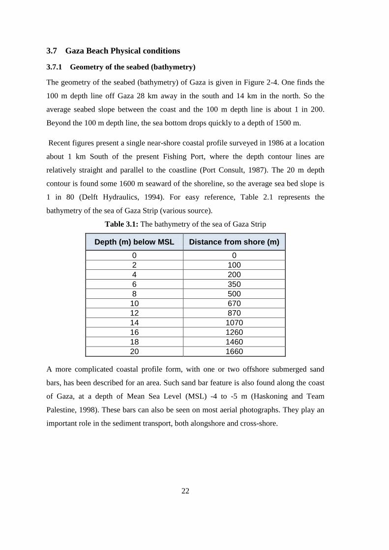
3.7.1 Geometry of the seabed (bathymetry)
The geometry of the seabed (bathymetry) of Gaza is given in Figure 2-4. One finds the
100 m depth line off Gaza 28 km away in the south and 14 km in the north. So the
average seabed slope between the coast and the 100 m depth line is about 1 in 200.
Beyond the 100 m depth line, the sea bottom drops quickly to a depth of 1500 m.
Recent figures present a single near-shore coastal profile surveyed in 1986 at a location
about 1 km South of the present Fishing Port, where the depth contour lines are
relatively straight and parallel to the coastline (Port Consult, 1987). The 20 m depth
contour is found some 1600 m seaward of the shoreline, so the average sea bed slope is
1 in 80 (Delft Hydraulics, 1994). For easy reference, Table 2.1 represents the
bathymetry of the sea of Gaza Strip (various source).
Table 3.1: The bathymetry of the sea of Gaza Strip
Depth (m) below MSL Distance from shore (m)
0 0
2 100
4 200
6 350
8 500
10 670
12 870
14 1070
16 1260
18 1460
20 1660
A more complicated coastal profile form, with one or two offshore submerged sand
bars, has been described for an area. Such sand bar feature is also found along the coast
of Gaza, at a depth of Mean Sea Level (MSL) -4 to -5 m (Haskoning and Team
Palestine, 1998). These bars can also be seen on most aerial photographs. They play an
important role in the sediment transport, both alongshore and cross-shore.
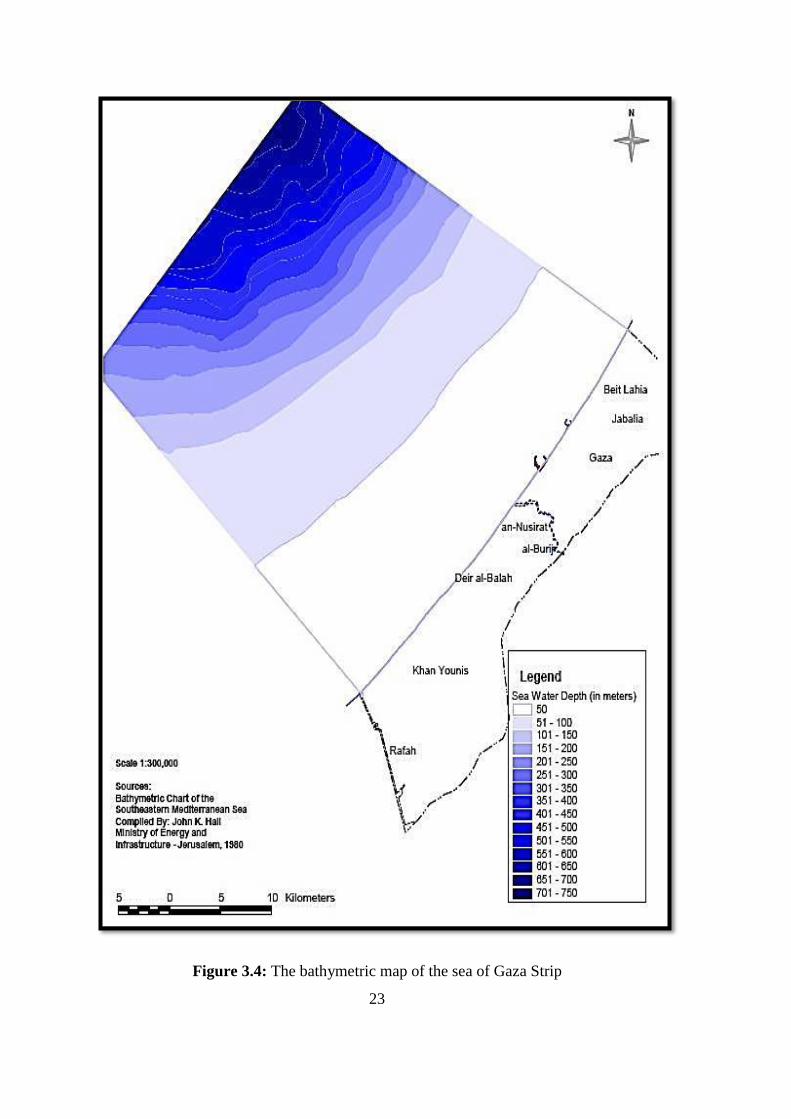
23
Figure 3.4: The bathymetric map of the sea of Gaza Strip

24
3.7.2 Water Level and Tides
The astronomical tidal range in the Mediterranean is small. From the Admiralty Tide
Tables of 1988 the following tidal levels were found in Table 2.2 (D. Hydraulic, 1994).
Table 3.2: Tidal ranges in Gaza Strip
Tide level Value(m)
HAT + 0.45
MHWS + 0.35
MHWN + 0.15
MSL 0
MLWN -0.15
MLWS -0.25
LAT -0.35
Where,
HAT: Highest Astronomical Tide.
MHWS: Mean High Water Springs.
MHWN: Mean High Water Neaps.
MLWS: Mean Low Water Springs.
MLWN: Mean Low Water Neaps.
LAT: Lowest Astronomical Tide.
Extreme water level variations are commonly caused by barometric pressure variations,
rather than by tides. These meteorological variations may often have more effect on the
sea level than tides. The design water level along the eastern Mediterranean coast is
taken as MSL + 1 m, which corresponds approximately with a water level which is
being exceeded once in 50 years (Matar et al, 2012).
3.7.3 Wind and Wave
The wave rose for year 2004-2005 at IDKU station in Egypt is illustrated in Figures 2.5
and 2.6 (Seif, 2011). Summary of wave conditions derived from IDKU station are
shown in Tables 2.3. Table 2.4 shows the presented wave scenarios for Gaza data
derived from Ashdod measurements (D. Hydraulic,1994). The waves in Gaza Strip are
considered swell waves, resulting from the wind, although there are some other waves
resulting from other climatic conditions but in small effects. The dominated waves are
from West-NorthWest (WNW) direction along year.
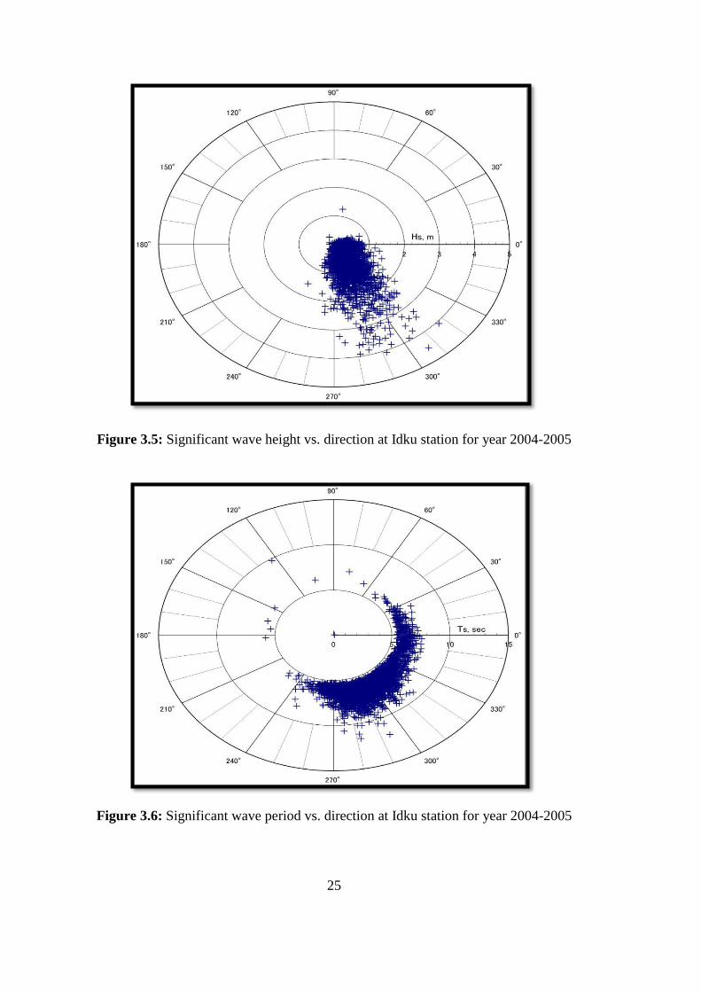
25
Figure 3.5: Significant wave height vs. direction at Idku station for year 2004-2005
Figure 3.6: Significant wave period vs. direction at Idku station for year 2004-2005

26
Table 3.3: Average yearly wave data at Idku station for year 2004-2005
Wave scenario
Hs [m] Ts [s] Direction
[deg.North]
Duration
[days]
H ≤ 1.0 m 0.5 6.3 284 289.0
1.0 > H ≤ 2.0 m 1.3 7.1 295 63.0
2.0 > H ≤3.0 m 2.4 8.0 293 10.0
3.0 > H ≤ 4.0 m 3.4 8.8 292 2.7
H < 4.0m 4.2 9.4 305 0.3
Hs: significant wave height; Ts: significant wave period; Direction is the wave direction; H: wave height
Table 3.4: Average yearly wave condition for Gaza from Ashdod station
Wave scenario
Hs [m] Ts [s] Direction
[deg.North]
Duration
[days]
H ≤ 1.0 m 0.67 5.9 342.0 197.1
1.0 > H ≤ 2.0 m 1.00 6.5 275.0 159.8
2.0 > H ≤3.0 m 2.25 7.9 323.0 1.80
3.0 > H ≤ 4.0 m 3.50 8.8 290.0 3.32
3.0 > H ≤ 4.0 m 3.55 8.8 268.8 2.92
Hs: significant wave height; Ts: significant wave period; Direction is the wave direction; H: wave height
3.7.4 Caostal Geology
Grabowski and Poort 1994 showed that the deposits of the Holocene and the Pleistocene
in Gaza terrestrial area are approximately 160 m thick, covering the underlying Pliocene
sediments. These deposits consist of marine kurkar formation, shell fragments and
quartz sands cemented together. Calcareous sandstone is also found in some areas. It
was found that the marine kurkar forms a good ground water aquifer where most of the
groundwater of Gaza Strip is extracted from this layer. The thickness of the marine
kurkar varies between 10 m and 100 m with a tendency thicker near the coast. The
formation of the continental kurkar is varied from friable to very hard, depending on the
degree of cementation. Alluvial and wind blown sand deposits are found on top of the
(Pleistocene) kurkar formations reaching a thickness of 25 m.
27
According to (Grabowski and Poort, 1994) four types of alluvial deposits can be
distinguished:
1. Sand dunes are oriented in the south near Rafah, mainly East-NorthEast (ENE)
to West-SouthWest (WSW). The north dunes become sporadic with scattered
sand in a zone of 2 to 3 km from the coast.
2. Wadi fillings consisting of sandy loess and gravel beds, which can reach a
thickness of 10 to 20 m.
3. Alluvial and aeolian deposits of varying thickness. In the northern part from the
Wadi Gaza aluvial deposits are widely distributed and are dominated by heavy,
loamy clay.
4. Beach formation consisting of a fairly thin layer of sand and shell fragments.
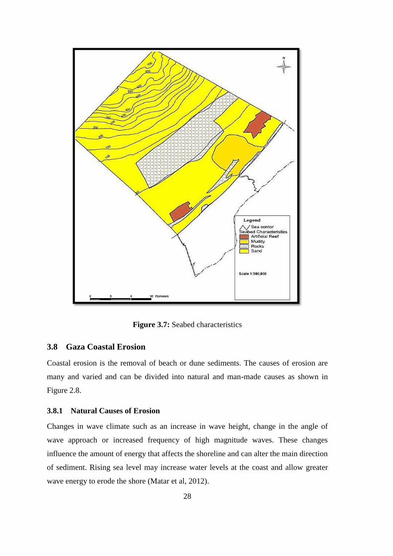
3.7.5 Coast and Seabed Characteristics
Going from sea to land, the coastal profile can be divided into the seabed, the beach, the
dune face or Kurkar (coarse sand) cliffs, and the adjacent body of the dune or cliff
plateau. The coastal profile does not only consist of sand, but locally also erosion
resistant formations of rock and Kurkar (coarse sand) protrude, on the seabed, on the
beach, and in the cliffs (Sogreah, 1996).
On the beach and near the waterline of the Gaza shoreline on many places Kurkar
(coarse sand) outcrops and rocky ridges can be seen. These hard ridges are important
coastal features in that they form natural breakwaters which tend to mitigate an eroding
trend. Where these hard layers are covered only by a relatively thin layer of sand, a
retreating coastal profile will gradually consist of an increasing amount of erosion-
resistant surface , as shown in Figure 2.7.
Defining the erodibility and composition of the steep Kurkar (coarse sand) cliffs along
the Gaza coastline is another important challenge. These cliffs themselves are to an
uncertain extent able to retard an erosion tendency. If they are attacked by waves and
locally collapse, the eroded coarse sand (Kurkar) material will feed the beach with a
mixture of very fine to very coarse sediment. The fines will soon be transported to deep
water, whereas the coarse particles will act as an armour layer, protecting the freshly
exposed coarse sand (Kurkar) cliff face during some time.
28
Figure 3.7: Seabed characteristics
3.8 Gaza Coastal Erosion
Coastal erosion is the removal of beach or dune sediments. The causes of erosion are
many and varied and can be divided into natural and man-made causes as shown in
Figure 2.8.
3.8.1 Natural Causes of Erosion
Changes in wave climate such as an increase in wave height, change in the angle of
wave approach or increased frequency of high magnitude waves. These changes
influence the amount of energy that affects the shoreline and can alter the main direction
of sediment. Rising sea level may increase water levels at the coast and allow greater
wave energy to erode the shore (Matar et al, 2012).
29
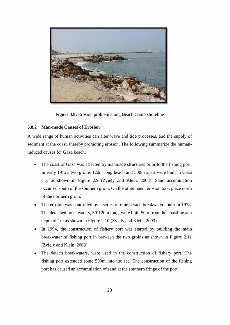
Figure 3.8: Erosion problem along Beach Camp shoreline
3.8.2 Man-made Causes of Erosion
A wide range of human activities can alter wave and tide processes, and the supply of
sediment at the coast, thereby promoting erosion. The following summarize the human-
induced causes for Gaza beach:
The coast of Gaza was affected by manmade structures prior to the fishing port.
In early 1972's two groins 120m long beach and 500m apart were built in Gaza
city as shown in Figure 2.9 (Zviely and Klein, 2003). Sand accumulation
occurred south of the southern groin. On the other hand, erosion took place north
of the northern groin.
The erosion was controlled by a series of nine detach breakwaters built in 1978.
The detached breakwaters, 50-120m long, were built 50m from the coastline at a
depth of 1m as shown in Figure 2.10 (Zviely and Klein, 2003).
In 1994, the construction of fishery port was started by building the main
breakwater of fishing port in between the two groins as shown in Figure 2.11
(Zviely and Klein, 2003).
The detach breakwaters, were used in the construction of fishery port. The
fishing port extended some 500m into the sea. The construction of the fishing
port has caused an accumulation of sand at the southern fringe of the port.

30
Figure 3.9: The two groins built in 1972
Figure 3.10: The detacher breakwaters built in 1978
Figure 3.11: The Fishing Port built in 1994
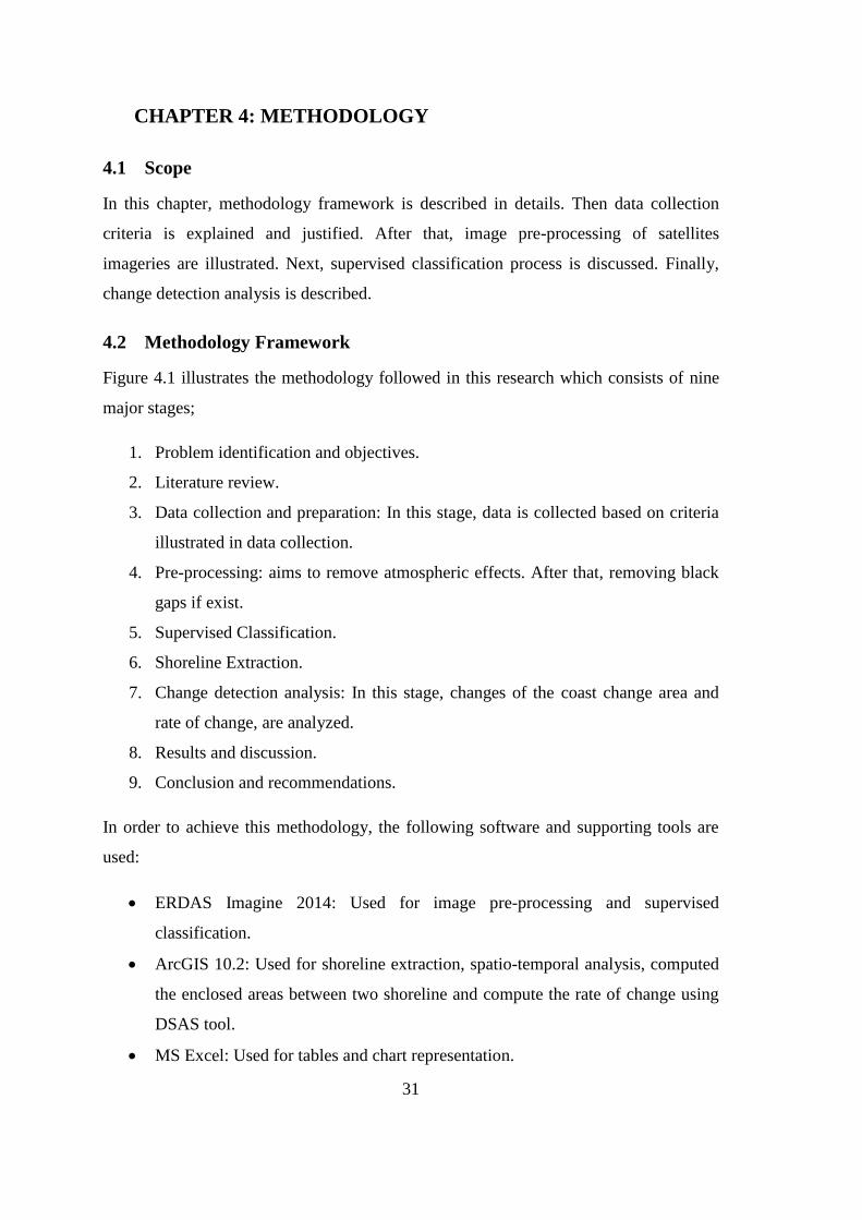
31
4 CHAPTER 4: METHODOLOGY
4.1 Scope
In this chapter, methodology framework is described in details. Then data collection
criteria is explained and justified. After that, image pre-processing of satellites
imageries are illustrated. Next, supervised classification process is discussed. Finally,
change detection analysis is described.
4.2 Methodology Framework
Figure 4.1 illustrates the methodology followed in this research which consists of nine
major stages;
1. Problem identification and objectives.
2. Literature review.
3. Data collection and preparation: In this stage, data is collected based on criteria
illustrated in data collection.
4. Pre-processing: aims to remove atmospheric effects. After that, removing black
gaps if exist.
5. Supervised Classification.
6. Shoreline Extraction.
7. Change detection analysis: In this stage, changes of the coast change area and
rate of change, are analyzed.
8. Results and discussion.
9. Conclusion and recommendations.
In order to achieve this methodology, the following software and supporting tools are
used:
ERDAS Imagine 2014: Used for image pre-processing and supervised
classification.
ArcGIS 10.2: Used for shoreline extraction, spatio-temporal analysis, computed
the enclosed areas between two shoreline and compute the rate of change using
DSAS tool.
MS Excel: Used for tables and chart representation.
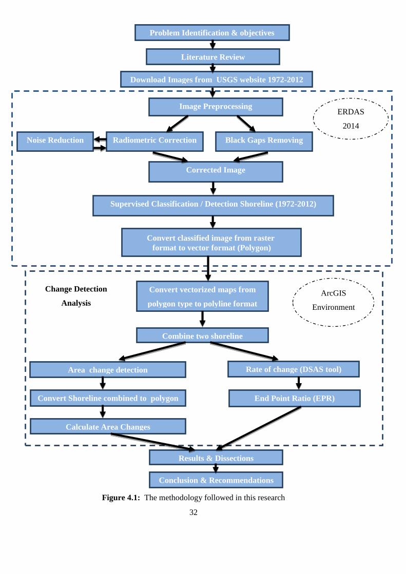
32
Figure 4.1: The methodology followed in this research
Problem Identification & objectives
Literature Review
Download Images from USGS website 1972-2012
Change Detection
Analysis
Convert vectorized maps from
polygon type to polyline format
Combine two shoreline
Area change detection Rate of change (DSAS tool)
Convert Shoreline combined to polygon
Calculate Area Changes
End Point Ratio (EPR)
ArcGIS
Environment
Image Preprocessing
Radiometric Correction Black Gaps Removing
Corrected Image
Noise Reduction
Supervised Classification / Detection Shoreline (1972-2012)
Convert classified image from raster
format to vector format (Polygon)
ERDAS
2014
Results & Dissections
Conclusion & Recommendations

33
4.3 Data Collection and Preparation
4.3.1 Data Collection
In this research, the data is mainly Landsat remotely sensed imageries downloaded from
U.S. Geological Survey (USGS) website – Landsat archive from 1972 to 2012.
The first criterion in data collection is to download even-year imageries, the time
between two image is not less than 4 year, including the oldest and newest Landsat
archived imageries, 1972 and 2012. The second criterion is to give TM imagery a
priority over ETM+ and/or MSS since TM sensor life span is longer than ETM+
(approx. 23 years) so consistent data will be collected. In contrast, Landsat ETM+
imageries have the problem of the Scan Line Corrector Failure (SLC-off) which
presented in black gaps. Moreover, Landsat ETM+ has the only advantage of the
panchromatic band existence. However, the resolution in the multispectral bands in
ETM+ is the same of TM, 30 m.
The third criterion is reducing the pre-processing by downloading all imageries in the
same date, month of September is chosen to avoid clouds in the scene. In case of
September imagery does not match the listed criteria, the closest imagery to September
matching the listed criteria will be downloaded. The fourth criterion is downloading a
full-bands imagery in a Geostationary Earth Orbit Tagged Image File Format
(GeoTIFF). In case of GeoTIFF does not available, the closest imagery to September
matching the listed criteria will be downloaded. The fifth criterion is downloading free
clouds scenes, at least above the study area. In case of cloud existence above the study
area, the closest imagery to September matching the listed criteria will be downloaded.
Based on these criteria, seven imageries are downloaded as illustrated in Table 4.1.
Table 4.1: Satellite image source and resolution
Image Source Date Resolution
(mxm) Image Source Date
Resolution
(mxm)
Landsat1 MSS 22-10-1972 60 x 60 Landsat5 TM 25-05-2002 30 x 30
Landsat5 TM 24-05-1984 30 x 30 Landsat7 ETM+ 26-09-2008 30 x 30
Landsat5 TM 14-09-1990 30 x 30 Landsat7 ETM+ 18-09-2012 30 x 30
Landsat5 TM 22-10-1998 30 x 30

34
4.3.2 Image Subset
A subset image was created from each image, which covers only the study area on each
date (1972-2012) by using ERDAS Imagine 2014 as shown in Appendix A1-7.
4.3.3 Image Pre-Processing
Preprocessing of image data often will include radiometric correction, geometric
correction and removing black gaps.
4.3.3.1 Geometric Correction
The images are projected to the Universal Transverse Mercator (UTM), with a spheroid
and datum of WGS 84. Landsat images were geometrically certificated.
To correct the geometric distortions, one should apply two steps, geo-referencing and
resampling using ArcGIS 10.2 or ERDAS 2014. After correcting the coordinate
system, the spatial characteristics of pixels may be changed. So resampling should be
applied to obtain a new image more pronounced in which all pixels are correctly
positioned within the terrain coordinate system to more accurate feature extraction
methods.
4.3.3.2 Radiometric Correction
Since digital sensors record the intensity of electromagnetic radiation from each spot
viewed on the Earth’s surface as a Digital Number (DN) for each spectral band, the
exact range of DN that a sensor utilizes depends on its radiometric resolution. For
example, a sensor such as Landsat MSS measures radiation on a 0-63 DN scale even as
Landsat TM and ETM+ measure it on a 0-255 scale (Green, et al., 2000). Radiometric
correction involves the processing of digital images to improve the fidelity of the
brightness value magnitudes. Any image contains radiometric errors and inconsistencies
will be referred to as "noise" these errors should be corrected before the extraction and
analysis of information from the image.
The sources of radiometric noise and therefore, the appropriate types of radiometric
corrections, partially depend on the sensor and mode of imaging used to capture the
digital image data such as satellite image, optical scanners, sensors and others.
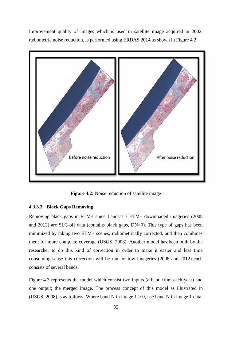
35
Improvement quality of images which is used in satellite image acquired in 2002,
radiometric noise reduction, is performed using ERDAS 2014 as shown in Figure 4.2.
Figure 4.2: Noise reduction of satellite image
4.3.3.3 Black Gaps Removing
Removing black gaps in ETM+ since Landsat 7 ETM+ downloaded imageries (2008
and 2012) are SLC-off data (contains black gaps, DN=0). This type of gaps has been
minimized by taking two ETM+ scenes, radiometrically corrected, and then combines
them for more complete coverage (USGS, 2008). Another model has been built by the
researcher to do this kind of correction in order to make it easier and less time
consuming sense this correction will be run for tow imageries (2008 and 2012) each
consists of several bands.
Figure 4.3 represents the model which consist two inputs (a band from each year) and
one output; the merged image. The process concept of this model as illustrated in
(USGS, 2008) is as follows: Where band N in image 1 > 0, use band N in image 1 data,

36
Otherwise, use band N in image 2. In other words, Image 2 data will fill the gaps in
Image 1. Black gap removing of satellite image acquired in 2008 shown in Figure 4.4.
Figure 4.3: Black gaps removing model
Figure 4.4: Black gap removing of satellite image
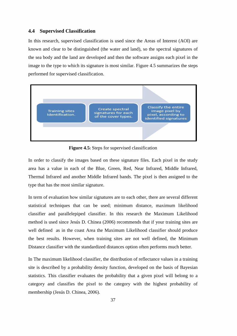
37
4.4 Supervised Classification
In this research, supervised classification is used since the Areas of Interest (AOI) are
known and clear to be distinguished (the water and land), so the spectral signatures of
the sea body and the land are developed and then the software assigns each pixel in the
image to the type to which its signature is most similar. Figure 4.5 summarizes the steps
performed for supervised classification.
Figure 4.5: Steps for supervised classification
In order to classify the images based on these signature files. Each pixel in the study
area has a value in each of the Blue, Green, Red, Near Infrared, Middle Infrared,
Thermal Infrared and another Middle Infrared bands. The pixel is then assigned to the
type that has the most similar signature.
In term of evaluation how similar signatures are to each other, there are several different
statistical techniques that can be used; minimum distance, maximum likelihood
classifier and parallelepiped classifier. In this research the Maximum Likelihood
method is used since Jesús D. Chinea (2006) recommends that if your training sites are
well defined as in the coast Area the Maximum Likelihood classifier should produce
the best results. However, when training sites are not well defined, the Minimum
Distance classifier with the standardized distances option often performs much better.
In The maximum likelihood classifier, the distribution of reflectance values in a training
site is described by a probability density function, developed on the basis of Bayesian
statistics. This classifier evaluates the probability that a given pixel will belong to a
category and classifies the pixel to the category with the highest probability of
membership (Jesús D. Chinea, 2006).
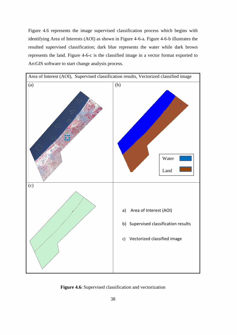
38
Figure 4.6 represents the image supervised classification process which begins with
identifying Area of Interests (AOI) as shown in Figure 4-6-a. Figure 4-6-b illustrates the
resulted supervised classification; dark blue represents the water while dark brown
represents the land. Figure 4-6-c is the classified image in a vector format exported to
ArcGIS software to start change analysis process.
Area of Interest (AOI), Supervised classification results, Vectorized classified image
(a)
(b)
(c)
a) Area of Interest (AOI)
b) Supervised classification results
c) Vectorized classified image
Figure 4.6: Supervised classification and vectorization
Water
Land

39
4.5 Shoreline Extraction
All most ArcGis 10.2 can extract the shoreline by using Arc Toolbox to convert the
polygon feature to line feature as shown in Figure 4.7, then the user should use editor
toolbar to remove the edge lines as shown in Figure 4.8, the remaining line which
separate two classify cluster represent shoreline. Finally user should repeat these step to
extract all shoreline Figure 4.9 show Gaza Strip shorelines from 1972-2012.
Figure 4.7: Convert polygon feature to line feature
Figure 4.8 : Extraction of shoreline
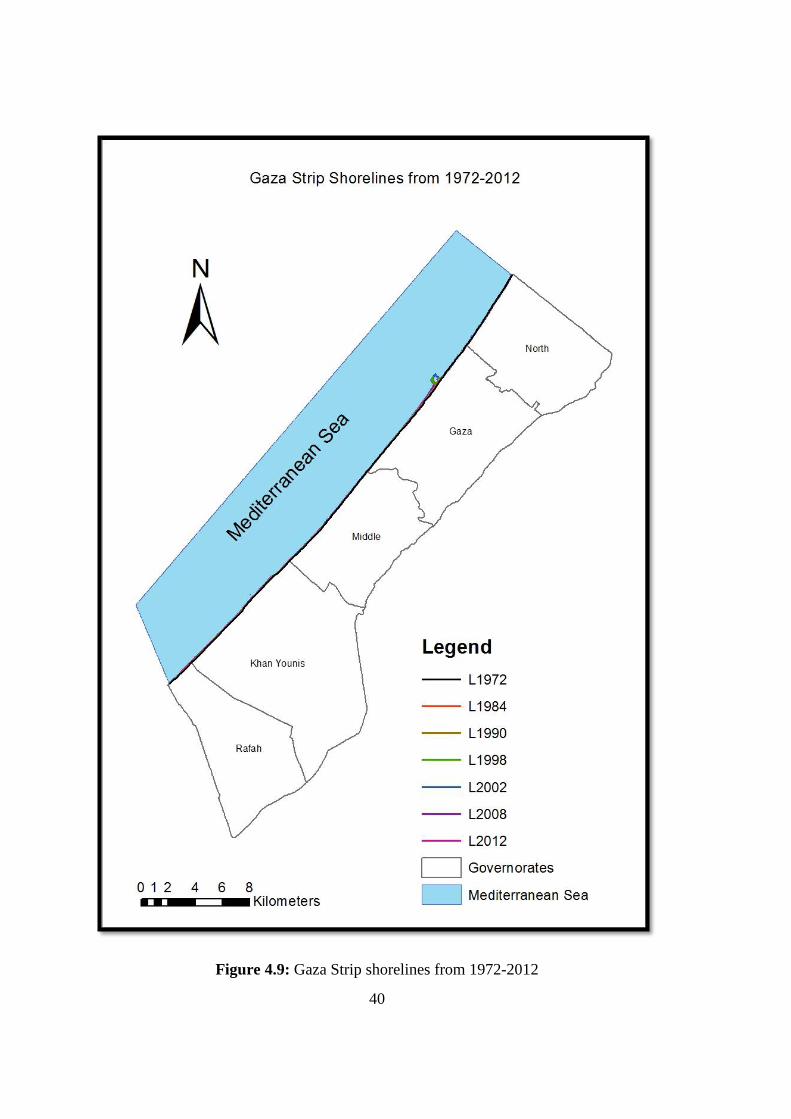
40
Figure 4.9: Gaza Strip shorelines from 1972-2012

41
4.6 Change Detection Analysis
In this stage, area and change rate detection analyses are done using ArcGIS tools.
4.6.1 Area Variation
In order to calculate the change in areas between different date, the ArcGIS tools was
used. First two different shorelines (line feature) should be appended in one feature
class by using Arc Toolbox as shown in Figure 4.10. Then by using Arc Toolbox to
convert feature to polygon to detect the change in areas. Figure 4.11 illustrate the
change in areas between 2002-2008.
Figure 4.10: Append two different shoreline
Figure 4.11: Change in Areas between 2002-2008
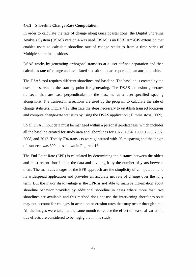
42
4.6.2 Shoreline Change Rate Computation
In order to calculate the rate of change along Gaza coastal zone, the Digital Shoreline
Analysis System (DSAS) version 4 was used. DSAS is an ESRI Arc-GIS extension that
enables users to calculate shoreline rate of change statistics from a time series of
Multiple shoreline positions.
DSAS works by generating orthogonal transects at a user-defined separation and then
calculates rate-of-change and associated statistics that are reported in an attribute table.
The DSAS tool requires different shorelines and baseline. The baseline is created by the
user and serves as the starting point for generating. The DSAS extension generates
transects that are cast perpendicular to the baseline at a user-specified spacing
alongshore. The transect intersections are used by the program to calculate the rate of
change statistics. Figure 4.12 illustrate the steps necessary to establish transect locations
and compute change-rate statistics by using the DSAS application ( Himmelstoss, 2009).
So all DSAS input data must be managed within a personal geodatabase, which includes
all the baseline created for study area and shorelines for 1972, 1984, 1990, 1998, 2002,
2008, and 2012. Totally 794 transects were generated with 50 m spacing and the length
of transects was 300 m as shown in Figure 4.13.
The End Point Rate (EPR) is calculated by determining the distance between the oldest
and most recent shoreline in the data and dividing it by the number of years between
them. The main advantages of the EPR approach are the simplicity of computation and
its widespread application and provides an accurate net rate of change over the long
term. But the major disadvantage is the EPR is not able to manage information about
shoreline behavior provided by additional shoreline in cases where more than two
shorelines are available and this method does not use the intervening shorelines so it
may not account for changes in accretion or erosion rates that may occur through time.
All the images were taken at the same month to reduce the effect of seasonal variation,
tide effects are considered to be negligible in this study.

43
Figure 4.12: Transect locations and change-rate using the DSAS
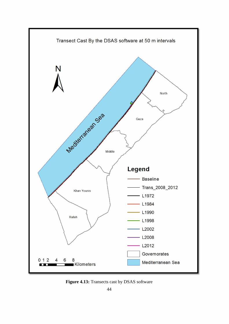
44
Figure 4.13: Transects cast by DSAS software

45
5 CHAPTER 5: RESULTS AND DISCUSSION
5.1 Scope
This chapter contains a detailed description of the steps of the methodology of the
research and illustrates the results of the detected changes in areas and rate of change of
the Gaza Strip coast over time.
5.2 Introduction
The shoreline in the study area has never been constant and shows a continuous
changing pattern . Both the spatial and temporal variations in the deposition and
accretion have been observed in the study area. The temporal intervals (being 1972
to 1984, 1984 to 1990, 1990 to 1998, 1998 to 2002, 2002 to 2008 and 2008 to 2012)
used in the study for assessing the changes have not been uniform. Based on the
results, Gaza Strip coastal zone could be classified into seven regions according to the
rate of change and governorates; such as: A) Rafah 2.4 km B) khan Younis 10.4 km C)
Southern of middle governorate 8 km D) El-Wadi region 2.4 km E) southern Sea port
6.4 km , F) northern sea port 3 km, and G) north Gaza governorate 6.2 km, as shown in
Figure 5.1.
The analysis of historical shoreline displacement is the understanding of the past, in
order to associate it with the present, and make forecasts about future shoreline
positions.

46
Figure 5.1: Gaza coastal zone classification
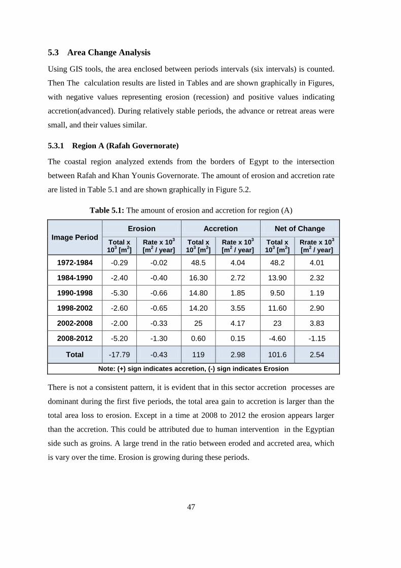
47
5.3 Area Change Analysis
Using GIS tools, the area enclosed between periods intervals (six intervals) is counted.
Then The calculation results are listed in Tables and are shown graphically in Figures,
with negative values representing erosion (recession) and positive values indicating
accretion(advanced). During relatively stable periods, the advance or retreat areas were
small, and their values similar.
5.3.1 Region A (Rafah Governorate)
The coastal region analyzed extends from the borders of Egypt to the intersection
between Rafah and Khan Younis Governorate. The amount of erosion and accretion rate
are listed in Table 5.1 and are shown graphically in Figure 5.2.
Table 5.1: The amount of erosion and accretion for region (A)
Image Period Erosion Accretion Net of Change
Total x 10
3 [m
2]
Rate x 103
[m2 / year]
Total x 10
3 [m
2]
Rate x 103
[m2 / year]
Total x 10
3 [m
2]
Rrate x 103
[m2 / year]
1972-1984 -0.29 -0.02 48.5 4.04 48.2 4.01
1984-1990 -2.40 -0.40 16.30 2.72 13.90 2.32
1990-1998 -5.30 -0.66 14.80 1.85 9.50 1.19
1998-2002 -2.60 -0.65 14.20 3.55 11.60 2.90
2002-2008 -2.00 -0.33 25 4.17 23 3.83
2008-2012 -5.20 -1.30 0.60 0.15 -4.60 -1.15
Total -17.79 -0.43 119 2.98 101.6 2.54
Note: (+) sign indicates accretion, (-) sign indicates Erosion
There is not a consistent pattern, it is evident that in this sector accretion processes are
dominant during the first five periods, the total area gain to accretion is larger than the
total area loss to erosion. Except in a time at 2008 to 2012 the erosion appears larger
than the accretion. This could be attributed due to human intervention in the Egyptian
side such as groins. A large trend in the ratio between eroded and accreted area, which
is vary over the time. Erosion is growing during these periods.

48
In general Rafah coastal area is being exposed to increase in the coastal areas at a rate
of 2,540 m2/year.
Figure 5.2: Average change rate for region A
5.3.2 Region B (Khan-Younis Governorate)
The coastal region analyzed extends from Rafah and Khan Younis Governorate. The
amount of erosion and accretion rate are listed in Table 5.2 and are shown graphically in
Figure 5.3.
Table 5.2: The amount of erosion and accretion for region (B)
Image period Erosion Accretion Net of Change
Total x 10
3 [m
2]
Rate x 103
[m2 / year]
Total x 10
3 [m
2]
Rate x 103
[m2 / year]
Total x 10
3 [m
2]
Rate x 103
[m2 / year]
1972-1984 -1.50 -0.13 178.08 14.84 176.58 14.72
1984-1990 -26.80 -4.47 58.00 9.67 31.20 5.20
1990-1998 -36.30 -4.54 51.15 6.39 14.85 1.86
1998-2002 -31.70 -7.93 35.30 8.83 3.60 0.90
2002-2008 -48.60 -8.10 82.20 13.70 33.60 5.60
2008-2012 -60.10 -15.03 12.70 3.18 -47.40 -11.85
Total -205.00 -5.13 417.43 10.44 212.43 5.31
Note: (+) sign indicates accretion, (-) sign indicates Erosion
0.00 1.00 2.00 3.00 4.00 5.00
1972-1984
1984-1990
1990-1998
1998-2002
2002-2008
2008-2012
Avreage Change rate 103 m2 /y
Region (A) / Average Change in Area (103 m2/year)
Erosion
Accretion
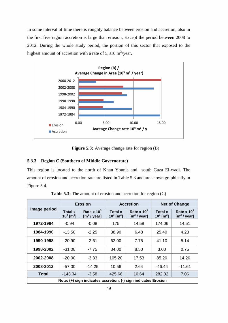
49
In some interval of time there is roughly balance between erosion and accretion, also in
the first five region accretion is large than erosion, Except the period between 2008 to
2012. During the whole study period, the portion of this sector that exposed to the
highest amount of accretion with a rate of 5,310 m2/year.
Figure 5.3: Average change rate for region (B)
5.3.3 Region C (Southern of Middle Governorate)
This region is located to the north of Khan Younis and south Gaza El-wadi. The
amount of erosion and accretion rate are listed in Table 5.3 and are shown graphically in
Figure 5.4.
Table 5.3: The amount of erosion and accretion for region (C)
Image period Erosion Accretion Net of Change
Total x 10
3 [m
2]
Rate x 103
[m2 / year]
Total x 10
3 [m
2]
Rate x 103
[m2 / year]
Total x 10
3 [m
2]
Rate x 103
[m2 / year]
1972-1984 -0.94 -0.08 175 14.58 174.06 14.51
1984-1990 -13.50 -2.25 38.90 6.48 25.40 4.23
1990-1998 -20.90 -2.61 62.00 7.75 41.10 5.14
1998-2002 -31.00 -7.75 34.00 8.50 3.00 0.75
2002-2008 -20.00 -3.33 105.20 17.53 85.20 14.20
2008-2012 -57.00 -14.25 10.56 2.64 -46.44 -11.61
Total -143.34 -3.58 425.66 10.64 282.32 7.06
Note: (+) sign indicates accretion, (-) sign indicates Erosion
0.00 5.00 10.00 15.00
1972-1984
1984-1990
1990-1998
1998-2002
2002-2008
2008-2012
Avreage Change rate 103 m2 / y
Region (B) / Average Change in Area (103 m2 / year)
Erosion
Accretion

50
Figure 5.4: Average change rate for region (C)
In the first five intervals the accretion is larger than the erosion. Except the last interval
between 2008-2012 is exposed to erosion larger than accretion. . During the whole
study period, the portion of this sector that exposed to the highest amount of accretion
with a rate of 7,000 m2 / year.
5.3.4 Region D (El-Wadi)
This region is located in the north of the Middle and Gaza governorates. The amount of
erosion and accretion rate are listed in Table 5.4 and are shown graphically in Figure
5.5.
Table 5.4: The amount of erosion and accretion for region (D)
Image period
Erosion Accretion Net of Change
Total x 10
3 [m
2]
Rate x 103
[m2 / year]
Total x 10
3 [m
2]
Rate x 103
[m2 / year]
Total x 10
3 [m
2]
Rate x 103
[m2 / year]
1972-1984 -21.00 -1.75 5.6 0.47 -15.40 -1.28
1984-1990 -35.00 -5.83 1.00 0.17 -34.00 -5.67
1990-1998 -23.44 -2.93 2.00 0.25 -21.44 -2.68
1998-2002 -21.90 -5.48 0.64 0.16 -21.26 -5.32
2002-2008 -0.45 -0.08 26.40 4.40 25.95 4.33
2008-2012 -19.80 -4.95 1.20 0.30 -18.60 -4.65
Total -121.59 -3.04 36.84 0.92 -84.75 -2.12
Note: (+) sign indicates accretion, (-) sign indicates Erosion
0.00 5.00 10.00 15.00 20.00
1972-1984
1984-1990
1990-1998
1998-2002
2002-2008
2008-2012
Avreage Change rate 103 m2 / y
Region (C) / Average Change in Area (103 m2 / year)
Erosion
Accretion

51
Figure 5.5: Average change rate for region (D)
The results show negative rates in general, which means that erosion was the
predominant process. Except the intervals 2002 to 2008 which show positive rates. The
main causes of erosion in this region due to Gaza valley (Gaza-Wadi). In general El-
Wadi region is being exposed to decrease in the coastal areas at a rate of 2,120 m2/year.
5.3.5 Region E (Southern Sea Port)
This region is located to the north of El-Wadi region to the south side of Gaza sea port.
The amount of erosion and accretion rate are listed in Table 5.5 and are shown
graphically in Figure 5.6.
Table 5.5: The amount of erosion and accretion for region (E)
Image Period Erosion Accretion Net of Change
Total x 10
3 [m
2]
Rate x 103
[m2 / year]
Total x 10
3 [m
2]
Rate x 103
[m2 / year]
Total x 10
3 [m
2]
Rate x 103
[m2 / year]
1972-1984 -0.10 -0.01 220 18.33 219.90 18.33
1984-1990 -12.50 -2.08 36.12 6.02 23.62 3.94
1990-1998 -16.00 -2.00 77.00 9.63 61.00 7.63
1998-2002 -2.20 -0.55 81.50 20.38 79.30 19.83
2002-2008 -5.30 -0.88 158.70 26.45 153.40 25.57
2008-2012 -5.70 -1.43 66.00 16.50 60.30 15.08
Total -41.80 -1.04 639.32 15.98 597.52 14.94
Note: (+) sign indicates accretion, (-) sign indicates Erosion
0.00 1.00 2.00 3.00 4.00 5.00 6.00
1972-1984
1984-1990
1990-1998
1998-2002
2002-2008
2008-2012
Avreage Change rate 103 m2 / y
Region (D) / Average Change in Area (103 m2 / year)
Erosion
Accretion

52
Figure 5.6: Average change rate for region (E)
It is evident that in this region accretion processes are dominant during the whole
periods, the total area gain to accretion is the largest where the erosion process is very
small. This could be attributed due to human activities such as: groins which built at the
early of seventy and Gaza sea port which completely constructed in 1998. These
structures have interrupted the prevailing north-ward flowing alongshore current;
consequently, its load of sediment has been deposited south of the structures. In
general this region is being exposed to increase in the coastal areas at a rate of 14,940
m2/year.
The results have proved again the expectation of previous studies, where the positive
rate have appeared in the southern side of the Gaza sea port.
5.3.6 Region F (Northern Sea Port)
This region extends from the north side of Gaza sea port to the North Governorate. The
amount of erosion and accretion rate are listed in Table 5.6 and are shown graphically in
Figure 5.7.
0.00 10.00 20.00 30.00
1972-1984
1984-1990
1990-1998
1998-2002
2002-2008
2008-2012
Avreage Change rate 103 m2 / y
Region (E) / Average Change in Area (103 m2 / year)
Erosion
Accretion

53
Table 5.6: The amount of erosion and accretion for region (F)
Image Period Erosion Accretion Net of Change
Total x 10
3 [m
2]
Rate x 103
[m2 / year]
Total x 10
3 [m
2]
Rate x 103
[m2 / year]
Total x 10
3 [m
2]
Rate x 103
[m2 / year]
1972-1984 -196.00 -16.33 ---- ---- -196.00 -16.33
1984-1990 -18.00 -3.00 4.50 0.75 -13.50 -2.25
1990-1998 -35.60 -4.45 2.00 0.25 -33.60 -4.20
1998-2002 -38.00 -9.50 10.00 2.50 -28.00 -7.00
2002-2008 -71.60 -11.93 0.50 0.08 -71.10 -11.85
2008-2012 -57.98 -14.50 18.00 4.50 -39.98 -10.00
Total -417.18 -10.43 35.00 0.88 -382.18 -9.55
Note: (+) sign indicates accretion, (-) sign indicates Erosion
Figure 5.7: Average change rate for region (F)
The results show negative rates in general, which means that erosion was the
predominant process this region . Gaza Sea port caused a serious damage to the northern
beach especially after removing the nine detached breakwaters. The study show that the
erosion is growing during this periods, and these pattern of change will treat the public
and private property. This study show the average rate of erosion about 9,550 m2/y.
0.00 5.00 10.00 15.00 20.00
1972-1984
1984-1990
1990-1998
1998-2002
2002-2008
2008-2012
Avreage Change rate 103 m2 / y
Region (F) / Average Change in Area (103 m2 / year)
Erosion
Accretion

54
The results have proved again the expectation of previous studies, where the negative
rate have appeared in the northern side of the coastal zone
5.3.7 Region G (North Governorate)
This region is located from the north side of Gaza governorate to the northern border of
Gaza strip. The amount of erosion and accretion rate are listed in Table 5.7 and are
shown graphically in Figure 5.8.
Table 5.7: The amount of erosion and accretion for region (G)
Image Period
Erosion Accretion Net of Change
Total x 10
3 [m
2]
Rate x 103
[m2 / year]
Total x 10
3 [m
2]
Rate x 103
[m2 / year]
Total x 10
3 [m
2]
Rate x 103
[m2 / year]
1972-1984 -75.50 -6.29 3.6 0.30 -71.90 -5.99
1984-1990 -28.00 -4.67 5.10 0.85 -22.90 -3.82
1990-1998 -40.00 -5.00 8.00 1.00 -32.00 -4.00
1998-2002 -35.00 -8.75 16.00 4.00 -19.00 -4.75
2002-2008 -31.20 -5.20 10.23 1.71 -20.97 -3.50
2008-2012 -34.23 -8.56 24.32 6.08 -9.91 -2.48
Total -243.93 -6.10 67.25 1.68 -176.68 -4.42
Note: (+) sign indicates accretion, (-) sign indicates Erosion
Figure 5.8: Average change rate for region (G)
0.00 2.00 4.00 6.00 8.00 10.00
1972-1984
1984-1990
1990-1998
1998-2002
2002-2008
2008-2012
Avreage Change rate 103 m2 / y
Region (G) / Average Change in Area (103 m2 / year)
Erosion
Accretion
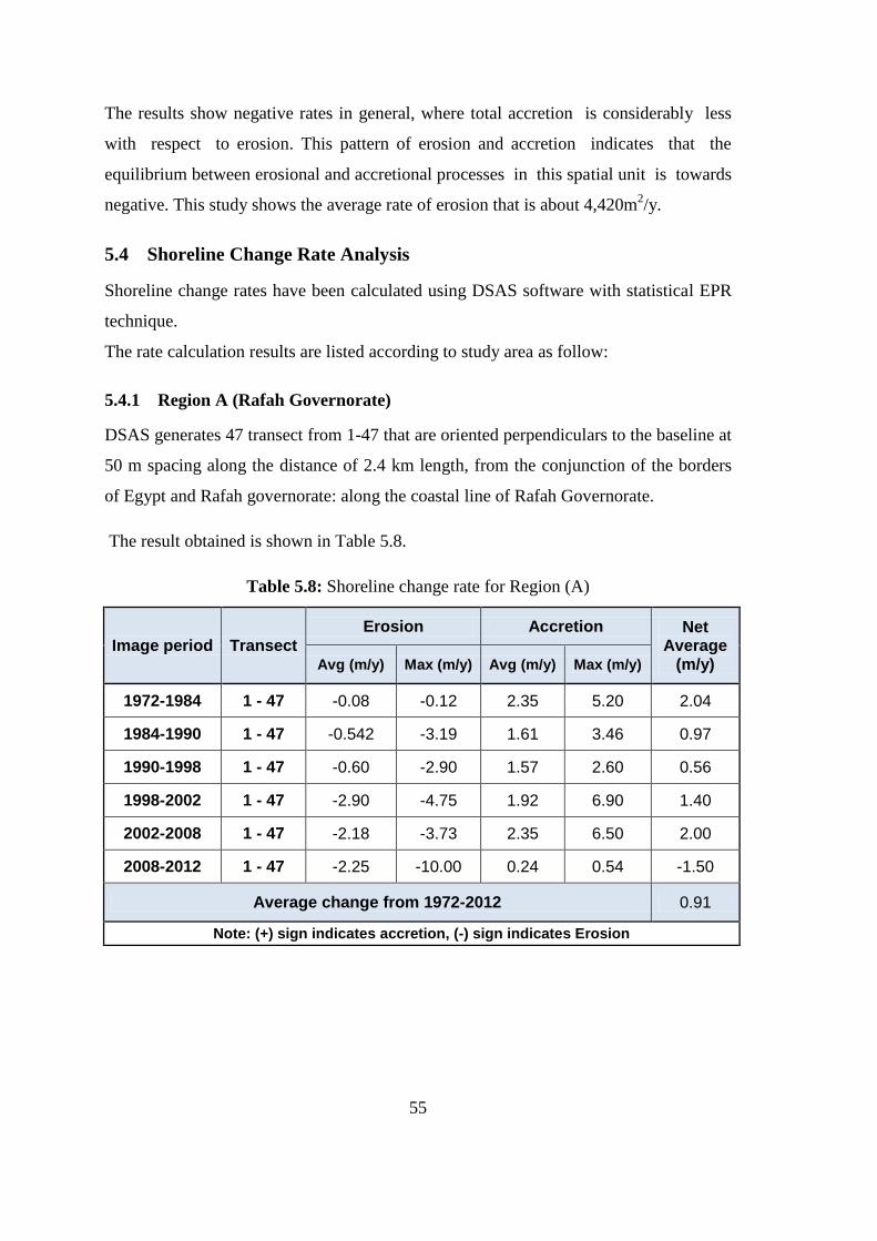
55
The results show negative rates in general, where total accretion is considerably less
with respect to erosion. This pattern of erosion and accretion indicates that the
equilibrium between erosional and accretional processes in this spatial unit is towards
negative. This study shows the average rate of erosion that is about 4,420m2/y.
5.4 Shoreline Change Rate Analysis
Shoreline change rates have been calculated using DSAS software with statistical EPR
technique.
The rate calculation results are listed according to study area as follow:
5.4.1 Region A (Rafah Governorate)
DSAS generates 47 transect from 1-47 that are oriented perpendiculars to the baseline at
50 m spacing along the distance of 2.4 km length, from the conjunction of the borders
of Egypt and Rafah governorate: along the coastal line of Rafah Governorate.
The result obtained is shown in Table 5.8.
Table 5.8: Shoreline change rate for Region (A)
Image period Transect Erosion Accretion Net
Average (m/y) Avg (m/y) Max (m/y) Avg (m/y) Max (m/y)
1972-1984 1 - 47 -0.08 -0.12 2.35 5.20 2.04
1984-1990 1 - 47 -0.542 -3.19 1.61 3.46 0.97
1990-1998 1 - 47 -0.60 -2.90 1.57 2.60 0.56
1998-2002 1 - 47 -2.90 -4.75 1.92 6.90 1.40
2002-2008 1 - 47 -2.18 -3.73 2.35 6.50 2.00
2008-2012 1 - 47 -2.25 -10.00 0.24 0.54 -1.50
Average change from 1972-2012 0.91
Note: (+) sign indicates accretion, (-) sign indicates Erosion
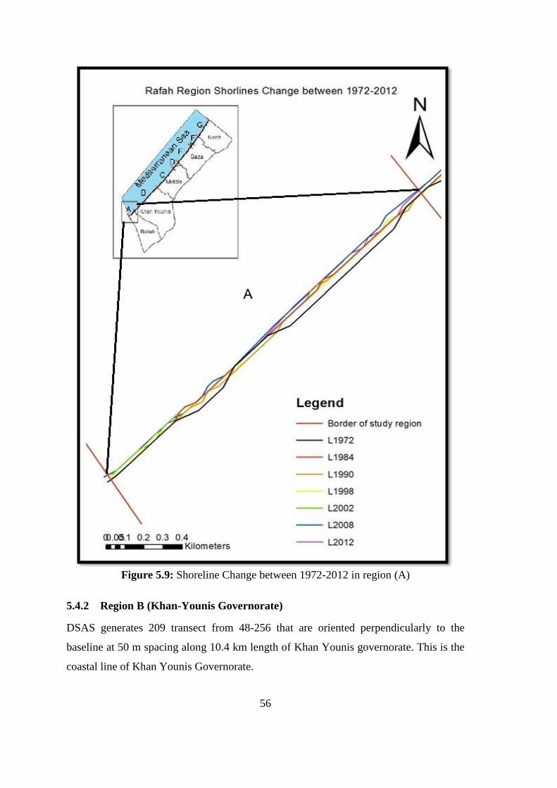
56
Figure 5.9: Shoreline Change between 1972-2012 in region (A)
5.4.2 Region B (Khan-Younis Governorate)
DSAS generates 209 transect from 48-256 that are oriented perpendicularly to the
baseline at 50 m spacing along 10.4 km length of Khan Younis governorate. This is the
coastal line of Khan Younis Governorate.

57
The result obtained is shown in Table 5.9.
Table 5.9: Shoreline change rate for Region (B)
Image period Transect Erosion Accretion Net
Average (m/y) Avg (m/y) Max(m/y) Avg (m/y) Max(m/y)
1972-1984 48 - 256 -0.17 -0.85 2.30 5.47 2.12
1984-1990 48 - 256 -1.14 -3.56 1.30 5.66 0.47
1990-1998 48 - 256 -0.71 -3.90 1.50 2.61 0.18
1998-2002 48 - 256 -3.00 -6.90 1.32 7.80 0.04
2002-2008 48 - 256 -0.40 -1.23 2.67 7.00 2.50
2008-2012 48 - 256 -2.15 -6.40 0.63 5.00 -1.18
Average Change from 1972-2012 0.69
Note: (+) sign indicates accretion, (-) sign indicates Erosion
5.4.3 Region C (Southern of Middle Governorate)
DSAS generates 159 transect from 257-415 that are oriented perpendicularly to the
baseline at 50 m spacing along 8 km length of South of the Middle Governorate. The
result obtained is shown in table 5.10.
Table 5.10: Shoreline change rate for Region (C)
Image period Transect Erosion Accretion Net
Average (m/y) Avg (m/y) Max(m/y) Avg (m/y) Max(m/y)
1972-1984 257-415 -0.12 -0.73 2.73 6.70 2.50
1984-1990 257-415 -0.83 -3.5 1.16 4.30 0.42
1990-1998 257-415 -0.56 -2.70 1.78 4.32 0.73
1998-2002 257-415 -2.50 -7.00 2.00 7.12 0.06
2002-2008 257-415 -0.90 -3.45 2.80 7.30 2.27
2008-2012 257-415 -3.30 9.80 0.98 6.70 -1.74
Average Change from 1972-2012 0.71
Note: (+) sign indicates accretion, (-) sign indicates Erosion
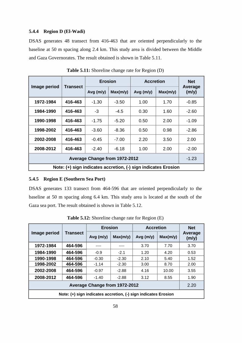
58
5.4.4 Region D (El-Wadi)
DSAS generates 48 transect from 416-463 that are oriented perpendicularly to the
baseline at 50 m spacing along 2.4 km. This study area is divided between the Middle
and Gaza Governorates. The result obtained is shown in Table 5.11.
Table 5.11: Shoreline change rate for Region (D)
Image period Transect Erosion Accretion Net
Average (m/y) Avg (m/y) Max(m/y) Avg (m/y) Max(m/y)
1972-1984 416-463 -1.30 -3.50 1.00 1.70 -0.85
1984-1990 416-463 -3 -4.5 0.30 1.60 -2.60
1990-1998 416-463 -1.75 -5.20 0.50 2.00 -1.09
1998-2002 416-463 -3.60 -8.36 0.50 0.98 -2.86
2002-2008 416-463 -0.45 -7.00 2.20 3.50 2.00
2008-2012 416-463 -2.40 -6.18 1.00 2.00 -2.00
Average Change from 1972-2012 -1.23
Note: (+) sign indicates accretion, (-) sign indicates Erosion
5.4.5 Region E (Southern Sea Port)
DSAS generates 133 transect from 464-596 that are oriented perpendicularly to the
baseline at 50 m spacing along 6.4 km. This study area is located at the south of the
Gaza sea port. The result obtained is shown in Table 5.12.
Table 5.12: Shoreline change rate for Region (E)
Image period Transect Erosion Accretion Net
Average (m/y) Avg (m/y) Max(m/y) Avg (m/y) Max(m/y)
1972-1984 464-596 ---- ---- 3.70 7.70 3.70
1984-1990 464-596 -0.9 -2.1 1.20 4.20 0.53
1990-1998 464-596 -0.30 -2.30 2.10 5.40 1.52
1998-2002 464-596 -1.14 -2.30 3.00 8.70 2.00
2002-2008 464-596 -0.97 -2.88 4.16 10.00 3.55
2008-2012 464-596 -1.40 -2.88 3.12 8.55 1.90
Average Change from 1972-2012 2.20
Note: (+) sign indicates accretion, (-) sign indicates Erosion
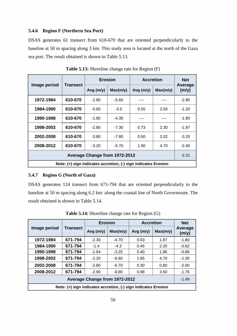
59
5.4.6 Region F (Northern Sea Port)
DSAS generates 61 transect from 610-670 that are oriented perpendicularly to the
baseline at 50 m spacing along 3 km. This study area is located at the north of the Gaza
sea port. The result obtained is shown in Table 5.13.
Table 5.13: Shoreline change rate for Region (F)
Image period Transect Erosion Accretion Net
Average (m/y) Avg (m/y) Max(m/y) Avg (m/y) Max(m/y)
1972-1984 610-670 -2.80 -5.60 ---- ---- -2.80
1984-1990 610-670 -0.65 -3.5 0.55 2.50 -1.20
1990-1998 610-670 -1.80 -4.30 ---- ---- -1.80
1998-2002 610-670 -2.80 -7.30 0.73 2.30 -1.87
2002-2008 610-670 -3.80 -7.80 0.50 2.02 -3.20
2008-2012 610-670 -3.20 -5.70 1.90 4.70 -2.40
Average Change from 1972-2012 -2.21
Note: (+) sign indicates accretion, (-) sign indicates Erosion
5.4.7 Region G (North of Gaza)
DSAS generates 124 transect from 671-794 that are oriented perpendicularly to the
baseline at 50 m spacing along 6.2 km: along the coastal line of North Governorate. The
result obtained is shown in Table 5.14.
Table 5.14: Shoreline change rate for Region (G)
Image period Transect Erosion Accretion Net
Average (m/y) Avg (m/y) Max(m/y) Avg (m/y) Max(m/y)
1972-1984 671-794 -2.30 -4.70 0.63 1.87 -1.80
1984-1990 671-794 -1.4 -4.3 0.45 2.20 -0.62
1990-1998 671-794 -1.64 -3.25 0.40 1.86 -0.86
1998-2002 671-794 -2.20 -6.60 1.85 4.70 -1.30
2002-2008 671-794 -2.80 -6.70 0.30 0.80 -2.60
2008-2012 671-794 -2.90 -8.80 0.98 3.50 -1.76
Average Change from 1972-2012 -1.49
Note: (+) sign indicates accretion, (-) sign indicates Erosion

60
The results which obtained above presented graphically in the following Figures from
5.10 to 5.15:
Figure 5.10: Annual shoreline change rate 1972-1984
Figure 5.11: Annual shoreline change rate 1984-1990
Figure 5.12: Annual shoreline change rate 1990-1998
-10
-5
0
5
10
0 50 100 150 200 250 300 350 400 450 500 550 600 650 700 750 800
Rat
e o
f C
han
ge (
m/y
)
Transect Number
Annual shoreline change rate 1972-1984 North
(B)
North
(E)
North
(D)
North
(C) (A)
(G) (F)
-8
-6
-4
-2
0
2
4
6
8
0 50 100 150 200 250 300 350 400 450 500 550 600 650 700 750 800
Rat
e o
f C
han
ge (
m/y
)
Transect Number
Annual shoreline change rate 1984-1990 North
-6
-4
-2
0
2
4
6
0 50 100 150 200 250 300 350 400 450 500 550 600 650 700 750 800
Rat
e o
f C
han
ge (
m/y
)
Transect Number
Annual shoreline change rate 1990-1998 North
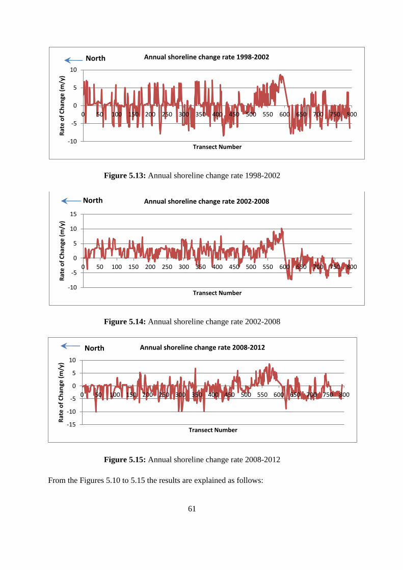
61
Figure 5.13: Annual shoreline change rate 1998-2002
Figure 5.14: Annual shoreline change rate 2002-2008
Figure 5.15: Annual shoreline change rate 2008-2012
From the Figures 5.10 to 5.15 the results are explained as follows:
-10
-5
0
5
10
0 50 100 150 200 250 300 350 400 450 500 550 600 650 700 750 800
Rat
e o
f C
han
ge (
m/y
)
Transect Number
Annual shoreline change rate 1998-2002 North
-10
-5
0
5
10
15
0 50 100 150 200 250 300 350 400 450 500 550 600 650 700 750 800
Rat
e o
f C
han
ge (
m/y
)
Transect Number
Annual shoreline change rate 2002-2008 North
-15
-10
-5
0
5
10
0 50 100 150 200 250 300 350 400 450 500 550 600 650 700 750 800
Rat
e o
f C
han
ge (
m/y
)
Transect Number
Annual shoreline change rate 2008-2012 North
62
For regions A, B, C they exposed to accretion in the first five periods, but the last
periods the erosion is being the large this is attributed to human activities especially the
groins which the Egyptian governorate build near to the Rafah borders.
Region D is expose to erosion in a whole periods of time, this unbalance due to the
influence of Gaza Valley.
Most substantial changes have been observed in the south side of Gaza sea port which
obtained positive rate, where Gaza seaport interrupts the natural movement of the
sediments along the coast.
Finally the region F,G , are expose to a serious problem of erosion especially the beach
camp.
63
6 CHAPTER 6: CONCLUSION AND RECOMMENDATIONS
6.1 Conclusion
Analysis of satellite Landsat images for the Mediterranean coast of Gaza strip for the
years from 1972 to 2012 have indicated shoreline changes in response to erosion and
accretion patterns. Based on the results, Gaza coastal zone could be classified into seven
regions according to the rate of change and governorates.
In this research seven satellite imageries (MSS, TM and +ETM Landsat) are collected
from 1972 to 2012. First all satellite images are radiometrically and atmospherically
Corrected using ERDAS Imagine 2014. Geographic Information system and Remote
Sensing techniques are used for spatio-temporal analysis in order to detect changes in
the shoreline position and the change in the coast areas. The analyses identified the
erosion and accretion patterns along the Gaza strip coast.
The results indicate that the regions A, B, C they expose to accretion in the first five
periods, but the last periods the erosion is being the large, the region D is expose to
erosion in a whole periods of time 1972-2012, the average annual erosion rates and rate
of change from 1972 to 2012 were 2,120 m2 and 1.23 m, respectively. Most substantial
changes have been observed in the south side of Gaza sea port (region E) which
obtained positive annual rate 14,940 m2 and change rate a bout 2.2 m. Region F expose
to a serious problem of erosion. The annual erosion rates is a bout 9,550 m2 and 2.2m.
Finally region G also expose to erosion patterns.
6.2 Recommendations
The study is greatly depends on the accuracy of environmental data and this leads to
uncertainty of the results from quantitative point of view. Therefore the following
recommendations should be taken into consideration for future study to enhance the
results:
Supporting researches and projects in this field from Palestinian universities.
Utilization of the result of this research in order to find strategies and solutions
to keep Gaza shoreline ―alive‖.
64
The stockholders should make periodic check on the critical region such as the
north of Gaza sea port and the south governorate of Gaza Strip which face a
serious problem.
Protect northern beach of Gaza city and Rafah which expose to a real threat and
could form a serious problem to structures which are near the beach such as:
Roads, restaurants, mosque and hotels.
Field measurements of wave characteristics should be carried out, which is
greatly affect the morphodynamic for Gaza coastal waters.
Bathometric survey should be carried out in regular basis to quantify
morphologic changes.
Recent satellite images are required to monitor the temporal shoreline changes.
To make the analysis more accurate, future studies should also consider tide
data, and data should be collected more frequently so that the change in the
shoreline can be observed more clearly.
Further studies will be carried out in order to calculate the volumetric change in
the southern side of Gaza sea port.
Using overlay analysis by using GIS environment to estimate the rate of
shoreline changes.
The study on the impact of marine tongue on the Egyptian border to the Gaza
Strip at the Rafah beach.
65
REFERENCES
Abu-Alhin, K., Niemeyer, I., 2009. Calculation of erosion and accretion rates along
Gaza coastal zone using remote sensing and geographic information system. 4th
EARSeL Workshop Remote Sensing of the Coastal Zone, Chania, Greece.
Abualtayef, M. Ghabayen, S. Abu Foul, A. Seif, A. Abd Rabou, A. Matar, O., 2013.
Mitigation measure for Gaza coastal erosion. J. Coastal Development Vol. 16 (2):135-
146.
Abualtayef, M. Ghabayen, S. Abu Foul, A. Seif, A. Kuroiwa, M. Matsubara, Y. Matar,
O., 2012. The impact pf Gaza fishing harbour on the Mediterranean coast of Gaza. J.
Coastal Development Vol. 16 (1):1-10.
Aedla, R. Dwarakish, G. S. Reddy, D. V., 2015. Automatic shoreline detection and
change detection analysis of Netravati Gurpur River mouth using histogram
equalization and adaptive thresholding techniques. (ICWRCOE), Aquatic Procedia 4 (
2015 ) 563 – 570.
Alemayehu, F. Richard, O. Kinyanjui, M. J., Oliverv,W., 2014. Assessment of
Shoreline Changes in the Period 1969-2010 in Watamuarea, Kenya.14(6).
Ali, M., 2002. The coastal zone of Gaza Strip-Palestine management and problems.
Presentation for Mama first kick-off meeting 11-13 March Paris.
Alves, A.L., Amaro, V.E., and Vital, H., 2003. Multitemporal analysis of multispectral
Landsat 5 Thematic Mapper images for monitoring and evaluation of coastal
morphodynamic on the Northeastern Coast of Brazil. Journal of Coastal Research, SI
(35) 279–283.
Anders F. and M. Byrnes. 1991. Accuracy of shoreline change rates determined from
maps and aerial photographs. Shore and Beach 59: 17-26.
Delft Hydraulics, 1994. Port of Gaza, basic engineering study, Final report, Part 11,
Coastal impact study, prepared for the Palestinian National Authority and the Ministry
of Economic affairs, the Netherlands, Sep. 1994
Dewidar, M.K. and Frihy, E.O., 2010. Automated techniques for quantification of beach
change rates using Landsat series along the North-eastern Nile Delta, Egypt. Journal of
Oceanography and Marine Science, 1(2): 28–39.
Dolan, R., Hayden, B.P., May, P., and May, S.K., 1980. The reliability of shoreline
change measurements from aerial photographs. Shore and Beach, 48(4), 22–29.
Falk, Michael, et al. 2011. A First Course on Time Series Analysis. University of
W• urzburg: s.n., 2011.

66
Frihy, O.E., Nasr, S.M., Hattab, M.M.EL and Raey, M.E.L., 1994, Remote sensing of
beach erosion along the Rosetta Promontory Northwestern Nile Delta, Egypt,
International Journal of Remote Sensing, 15 (8), 1649-1660.
Fromard, F., Vega, C., and Proisy, C., 2004. Half a century of dynamic coastal change
affecting mangrove shorelines of French Guiana. A case study based on remote sensing
data analyses and field surveys. Marine Geology, 208: 265–280.
Grabowski & Poort, 1994. Port of Gaza. Basic Engineering Study, Part 10,
Environmental study, Final, Nov. 1994.
Green, Edmund P., et al. 2000. Remote Sensing Handbook for Tropical Coastal
Management. 2000.
Grigio, A.M., Amaro, V.E., Vital, H., and Diodato, M.A., 2005. A method for coastline
evolution analysis using GIS and remote sensing – A case study from the Guamare City,
Northeast Brazil. Journal of Coastal Research, SI (42): 412–421.
Haskoning and Team Palestine, 1998. Beach Camp shore protection project: preparation
for detailed design and tender document, June 1998.
Himmelstoss, E.A., Zichichi, J.L., and Ergul, Ayhan. 2009 Digital Shoreline Analysis
System (DSAS) version 4.0 — An ArcGIS extension for calculating shoreline change:
U.S. Geological Survey Open-File Report 2008-1278. *updated for version 4.3.
Jesús D. Chinea. 2006. Supervised classification. Universidad de Puerto Rico, Recinto
Universitario de Mayagüez. [Online] 2006. [Cited: 3 7, 2013.]
http://www.uprm.edu/biology/profs/chinea/gis/lectesc/tut4_3.pdf.
Jianya, Gong, et al. 2008. A review of multi-temporal remote sensing data change
detection algorithms. Hong Kong : The International archives of the photogrammetry,
remote sensing and spatial information sciences, 2008. Vol. XXXVII.
Kaliraj, S., Chandrasekar, N., Magesh, N. S., 2013. Evaluation of coastal erosion and
accretion processes along the southwest coast of Kanyakumari, Tamil Nadu using
geospatial techniques. Arabian Journal of Geosciences ISSN 1866-7511.
Kandare, Kaja. 2000. The time series change detection methods of remote sensing.
2000.
Komar, P.D., 1998. Beach processes and sedimentation. Upper Saddle River, New
Jersey: Prentice Hall Inc., 544p.
Kumaravel, S. Ramkumar, T. Gurunanam, B. Suresh, M. and Dharanirajanm, K., 2013
An application of remote sensing and GIS based shoreline change studies – A case
study in the cuddalore district, east coast of Tamilnadu, South India. International
journal of innovative technology and exploring Engineering (IJITEE) ISSN: 2278-3075,
Volume-2, Issue-4
Li R. 1998. Potential of high-resolution satellite imagery for national mapping
products. Photogrammetric Engineering and Remote Sensing 64(12):1165-1169.
67
LIST, J H. and Farris, A. S., 1999. Large-scale shoreline response to storms and fair
weather. Proceedings of the Coastal Sediments ’99 (Long Island, New York), pp. 1324–
1337.
Liu H. and K. Jezek. 2003. Automated extraction of coastline from satellite imagegery
by integrating Canny edge detector and locally adaptive thresholding method.
International Journal of Remote Sensing (in press).
Mageswaran, T., Ram M. V., Chenthamil S. S., Arumugam T., Tune U., and Kankara
R.S., 2015.Assessment of shoreline changes along Nagapattinam coast using geospatial
techniques. International journal of geomatics and geosciences Volume 5, No 4.
Matar, O., R. Alhourani, I. Alsheikh and S. Matar.2012. Mitigation measure for Gaza
coastal erosion. B.Sc. thesis, Islamic University, Gaza, Palestine.
Morton, R.A., 1991. Accurate shoreline mapping: past, present, and future. Proceedings
of the Coastal Sediments ’91 (Seattle, Washington), pp. 997–1010.
Mousavi, S.R., Shabani, M., Pasha, M., Rezaei, M., Yadollahi, A.K., 2007.
Morphological changes of Sefidrud delta, north Iran, using remote sensing and GIS
techniques. Proceedings of the 3rd International Conference on Recent Advances in
Space Technologies, RAST 2007, pp. 687–691.
Muslim, A.M., Ismail, K.L., Khalil, I., Razman, N., Zain, K., 2004. Detection of
shoreline changes at Kuala Terengganu, Malaysia from multi-temporal Satellite Sensor.
Palestinian National Authority, Ministry of Environmental affairs. Gaza Coastal and
Marine Environmental Protection and Management Action Plan, 2000.
Port Consult, 1987. Assistance to the fishermen, Gaza Strip. Final report of study on
fishery port - Gaza, Sept. 1987. Portconsult, Consulting Engineers A/S, Copenhagen.
Reinert, Gesine. 2010. Time Series. 2010.
Ritchie W., M. Wood, R. Wright and D. Tait. 1988. Surveying and Mapping for Field
Scientists. Longman, Harlow: New York.
Ryu J-H., J-S. Won and K. Min. 2002. Waterline extraction from Landsat TM data in
tidal flat. Remote Sensing of Environment 83: 442-456.
Scott, J., Reed, M. and Moore L., 2002. Using Landsat 7 images to derive a land-water
boundary in Southern Louisiana, technical report, Mid-Continent mapping Center, U.S.
Geological Survey
Scott, J.W., Moore, L.R., Harris, W.H. and Reed, M.D., 2003. Using Landsat 7
Enhanced Thematic Mapper Tasseled Cap Transformation to extract shoreline. U.S.
Geological Survey Open-File Report of 03-272.
Seif, A.,2011. Numerical simulation of 3D morphodynamic around coastal structures
using quasi-3D nearshore current model. Doctorate thesis, Tottori university, 2011.
68
Shaoqing, Zhang. 2008. The comparative study of three methods of remote sensing
image change detection. china : s.n.
Siddiqui, M.N., and Maajid, S., 2004. Monitoring of geomorphological changes for
planning reclamation work in coastal area of Karachi, Pakistan. Advances in Space
Research, 33, 1200–1205.
Singh, A. 1989. Digital change detection techniques using remotely-sensed data. s.l.
:Taylor & Francis, 1989.
Smith, G.L. and Zarillo, G.A., 1990. Calculating long-term shoreline recession rates
using aerial photographic and beach profiling techniques. Journal of Coastal Research,
6(1), 111–120.
Sogreah. Gaza Port- Part II Layout Report, Section II Site Conditions Study. Soghreah
Ingenieri, 1996.
Théau, Jérôme. 2012. Change detection. [ed.] David M. Danko Wolfgang Kresse.
Springer Handbook of Geographic Information. New york : Springer, 2012, 7.
Thieler E.R. and W. Danforth. 1994. Historical shoreline mapping (I): Techniques and
reducing positioning errors. Journal of Coastal Research 10(3): 549-563.
Wang, Y., and Koopmans, B.N., 1993, The topographic mapping of the tidal flats using
remote sensing and GIS techniques: A case study in the Wadden Sea area, Netherland,
Proceedings of International Symposium of Operationalization of Remote Sensing, 193-
203.
White K., El Asmar H., 1999. Monitoring changing position of coastlines using
thematic Mapper imagery, an example from the Nile Delta. Geomorphology 29: 93-105.
White, K., and El Asmar, H.M., 1999. Monitoring changing position of coastlines using
thematic mapper imagery, an example from the Nile delta. Geomorphology, 29: 93–
105.
Zakariya, R., Rosnan, Y., Saidin, S.A., Yahaya, M.H., Kasawani, I., and Lokman, H.,
2006. Shoreline detection and changes for Terengganu River mouth from satellite
imagery (Landsat 5 and Landsat 7). Journal of Sustainability Science and Management,
1 (1): 47–57.
Zviely, D. and M. Klein. 2003. The environmental impact of the Gaza Strip coastal
constructions. J.Coast.Res.Vol. 19 (4):1122-1127.
https://en.wikipedia.org/wiki/Longshore_drift
.ؼخ اإلسالخ غضح, فسطاجب سبح لطبع غضح "دساسخ جىىسفىجخ".سسبخ بجسزش, .3122هجخ. اجب,

69
APPENDIX A: Satellite Landsat Images Subset from 1972-2012
Figure A1: Subset for 1972

70
Figure A2: Subset for 1984

71
Figure A3: Subset for 1990
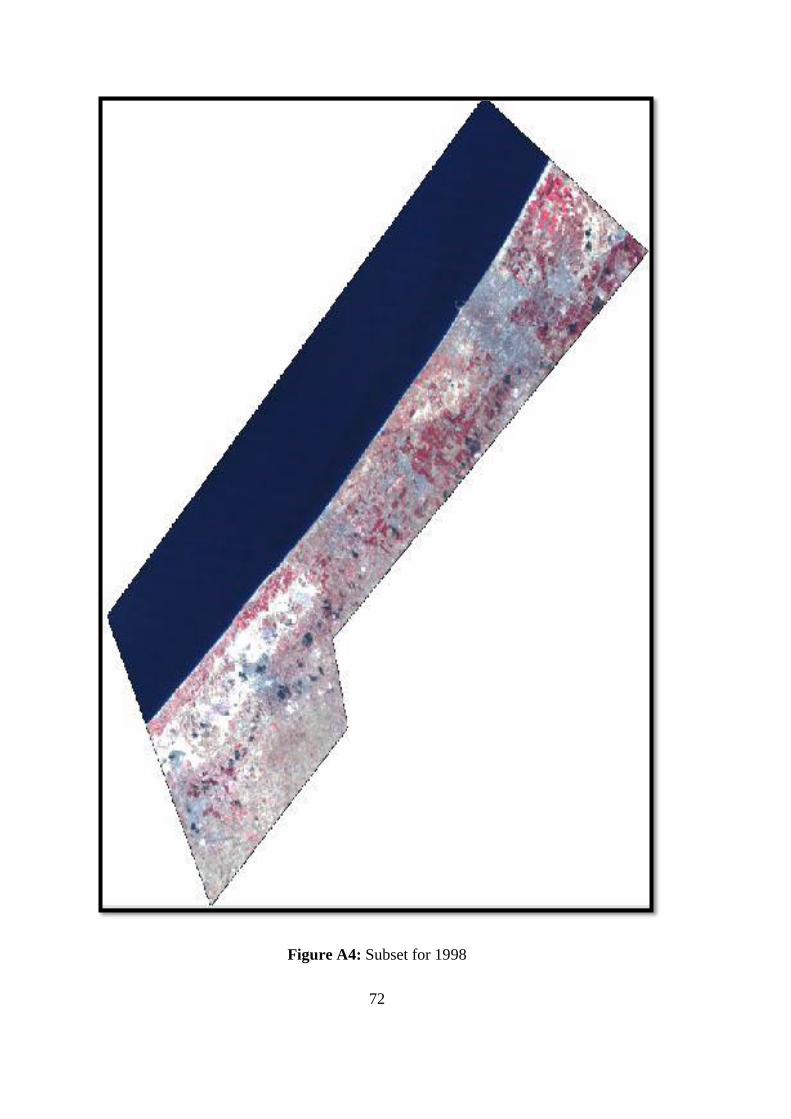
72
Figure A4: Subset for 1998

73
Figure A5: Subset for 2002

74
Figure A6: Subset for 2008

75
Figure A7: Subset for 2012