time response of linear dynamical systems in state space form

Lecture – 18

Time Response of Linear Dynamical Systems in State Space Form

Dr. Radhakant PadhiAsst. Professor

Dept. of Aerospace EngineeringIndian Institute of Science - Bangalore

ADVANCED CONTROL SYSTEM DESIGN Dr. Radhakant Padhi, AE Dept., IISc-Bangalore

2

Solution of Linear Differential Equations

Linear systems:Systems that obey the “Principle of superposition”.

Uniqueness Theorem:There is only one solution for linear systems.


3

Solution of Homogeneous Linear Differential Equation: Scalar caseSystem dynamics:Solution:

Initial condition:

Hence,

00 )(, xtxaxx ==( )

( )

/ln lnln /

at

dx x a dtx a t cx c a t

x e c

=

= +

=

=0 0

0 0,at atx e c c e x−= =

0)( 0)( xetx tta −=


4

Note:2 2 3 3

12! 3!

at a t a te at= + + + +

0

0

If 0, then the solution is( ) at

tx t e x

=

=

Solution of Homogeneous Linear Differential Equation: Scalar case


5

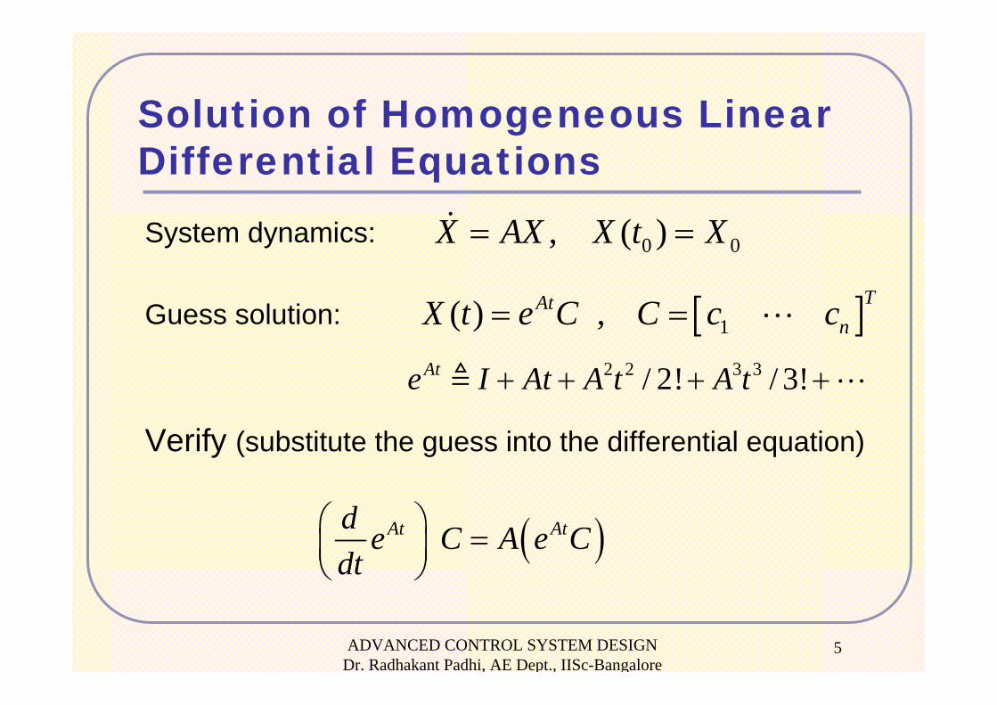
Solution of Homogeneous Linear Differential EquationsSystem dynamics:

Guess solution:

Verify (substitute the guess into the differential equation)

0 0, ( )X AX X t X= =

[ ]1( ) , TAtnX t e C C c c= =

2 2 3 3/ 2! / 3!Ate I At A t A t+ + + +

( )At Atd e C A e Cdt

⎛ ⎞ =⎜ ⎟⎝ ⎠


6

Solution of Homogeneous Linear Differential EquationsA Result:

i.e.

( ) ( ) ( )( )

2 2 3 3

2 3 2

2 2 3 3

/ 2! / 3!

0 2 / 2! 3 / 3!

/ 2! / 3!

At

At

At

e I At A t A td e A A t A tdt

A I At A t A t

Ae

= + + + +

= + + + +

= + + + +

=

( ) ( )At AtAe C A e C=

Therefore ( ) is 'a' solution.Hence, ( ) is 'the' solution.

At

At

X t e CX t e C

=

=


7

Solution of Homogeneous Linear Differential Equations

Applying the initial condition

Another result:(easy to show from definition)

Taking

Thus

Finally

0

0

0

1

0

At

At

X e C

C e X−

=

⎡ ⎤= ⎣ ⎦

( ) 0 0( )0 0

At A t tAtX t e e X e X− −= =

( )1 2 1 2A t t At Ate e e+ =

1 0 2 0 and ,t t t t= = − 0 0At AtI e e−=0 0

1At Ate e− −⎡ ⎤ =⎣ ⎦


8

Non-homogeneous system:

Solution contains two parts:• Homogeneous solution• Particular solution

Homogeneous solution:

Particular solution:

00 )(, XtXBUAXX =+=

( ) ( )AtpX t e C t=

0( )0( ) A t t

hX t e X−=

Solution of Non-homogeneous Linear Differential Equations


9

1

1

( )

( ) ( ) ( )

( )

tAt At A

pt

tA t

t

X t e C t e e BU d

e BU d

τ

τ

τ τ

τ τ

−

−

= =

=

∫

∫


1

( ) ( )

At At Atp

At

tA

t

X e C Ae C Ae C BU

C e BU

C t e BU dτ τ τ

−

−

= + = +

=

= ∫


10

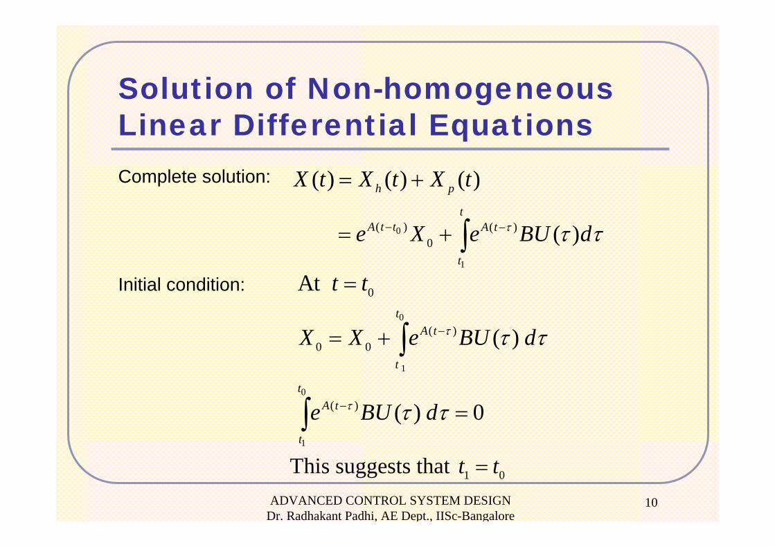
Complete solution:

Initial condition:

0

1

( ) ( )0

( ) ( ) ( )

( )

h p

tA t t A t

t

X t X t X t

e X e BU dτ τ τ− −

= +

= + ∫

0

1

0

1

0

( )0 0

( )

At

( )

( ) 0

tA t

t

tA t

t

t t

X X e BU d

e BU d

τ

τ

τ τ

τ τ

−

−

=

= +

=

∫

∫1 0This suggests that t t=



11

Complete solution:

The integral term in the forced system solution is a convolution integral.

Note: If is in feedback form

τττ dBUeXetXt

t

tAttA )()(0

0 )(0

)( ∫ −− +=

( )0( )

0( ) CL

CL

A t t

X A BK X A X

X t e X−

= − =

=

U ( )U K X= −



12

Solution of Non-homogeneous Linear Differential Equations:Some Comments

0

0

The solution results do not demand that .They are equally valid even if .

t tt t

≥≤

The integral term in the forced system solution is a "convolution integral".i.e. The contribution of input ( ) is the convolution of ( ) with .Hence, the function has the role of "impulse r

At

At

U t U t e Be B esponse" of the system

whose output is ( ) and input is ( ).X t U t

The solution for output ( ) is also readily available from ( ) and ( ) :( ) ( ) ( )

Y t X t U tY t CX t DU t= +


13

Example: Motion of a car without frictionThe equation of motion is

( )

0

0

( )1/ ( ) Assumption: is constant.

0 1 0( ), (0)

0 0 1/A B

m x f tx m f t m

v xxx x

X f t Xvv v m

=

=

⎡ ⎤⎡ ⎤ ⎡ ⎤ ⎡ ⎤ ⎡ ⎤= = + = ⎢ ⎥⎢ ⎥ ⎢ ⎥ ⎢ ⎥ ⎢ ⎥⎣ ⎦ ⎣ ⎦ ⎣ ⎦ ⎣ ⎦ ⎣ ⎦


14

Example: Motion of a car without friction

( )0

0

22

( )

( )

( ) ( )

1 0 0 1 10 1 0 0 0 12!

10 1

1 0 10 1 1/ 1

tAt A t

At

A t

A t

X t e X e B f d

tte I At A t

te

t te B

m m

τ

τ

τ

τ τ

τ

τ τ

−

−

−

= +

⎡ ⎤ ⎡ ⎤ ⎡ ⎤= + + + = + =⎢ ⎥ ⎢ ⎥ ⎢ ⎥

⎣ ⎦ ⎣ ⎦ ⎣ ⎦−⎡ ⎤

= ⎢ ⎥⎣ ⎦

− −⎡ ⎤ ⎡ ⎤ ⎡ ⎤= =⎢ ⎥ ⎢ ⎥ ⎢ ⎥⎣ ⎦ ⎣ ⎦ ⎣ ⎦

∫


15

Example: Motion of a car without friction

0 0 00 0

0 00 0

1 1( ) ( ) ( ) ( )( )( ) 1 1( ) ( )

t t

t t

x v t t f d x v t t f dm mx t

v tv f d v f d

m m

τ τ τ τ τ τ

τ τ τ τ

⎡ ⎤ ⎡ ⎤+ + − + −⎢ ⎥ ⎢ ⎥⎡ ⎤ ⎢ ⎥ ⎢ ⎥= =⎢ ⎥ ⎢ ⎥ ⎢ ⎥⎣ ⎦ + +⎢ ⎥ ⎢ ⎥

⎢ ⎥ ⎢ ⎥⎣ ⎦ ⎣ ⎦

∫ ∫

∫ ∫

⎥⎥⎦

⎤

⎢⎢⎣

⎡=

⎥⎥⎦

⎤

⎢⎢⎣

⎡

+

−++=⎥⎦

⎤⎢⎣

⎡

at

at

atv

attatvxtvtx 2

0

2

00 21

2)(

)()(

( ) /f t m a=Special case: (constant) and ⎥⎦

⎤⎢⎣

⎡=⎥

⎦

⎤⎢⎣

⎡00

0

0

vx


16

Evaluation of :A Useful Result

Ate

( )( )

( )

0

0

1

0

110

( ) ( )( )

( )

( )

sX s X A X ssI A X s X

X s sI A X

X t L sI A X

−

−−

− =

− =

= −

⎡ ⎤= −⎣ ⎦

0, (0)X A X X X= =Problem:

Solution using Laplace transform:

Solution known:

0( ) AtX t e X=

Comparing the two solutions:

( ) 11Ate L sI A −− ⎡ ⎤= −⎣ ⎦


17

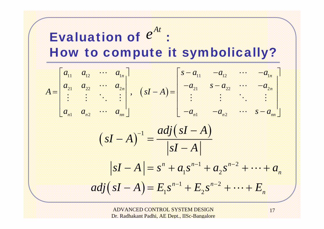
Evaluation of :How to compute it symbolically?

Ate

( )

11 12 1 11 12 1

21 22 2 21 22 2

1 2 1 2

,

n n

n n

n n nn n n nn

a a a s a a aa a a a s a a

A sI A

a a a a a s a

− − −⎡ ⎤ ⎡ ⎤⎢ ⎥ ⎢ ⎥− − −⎢ ⎥ ⎢ ⎥= − =⎢ ⎥ ⎢ ⎥⎢ ⎥ ⎢ ⎥− − −⎣ ⎦ ⎣ ⎦

( ) ( )

( )

1

1 21 2

1 21 2

n n nn

n nn

adj sI AsI A

sI A

sI A s a s a s a

adj sI A E s E s E

−

− −

− −

−− =

−

− = + + + +

− = + + +


18

Symbolic computation ofAte

( )( )( )

( ) ( )

1 21 2

1 21 2

1 21 2

11 2 1 1

n n nn

n nn

n n nn

n nn n n

I s a s a s a

sI A E s E s E

s I a s I a s I a Is E s E AE s E AE AE

− −

− −

− −

−−

+ + + +

= − + + +

+ + + +

= + − + + − −

( )( )( )( )1 2

1 1 2

1 11 2

n nn

n n nn

sI A E s E s EsI A sI A

s a s a s a

− −−

− −

− + + +− − =

+ + + +

Equate the coefficients on both sides…


19

Symbolic computation ofAte

1

2 1 1

3 2 2

1 1n n n

n n

E IE AE a IE AE a I

E AE a IAE a I

− −

=− =− =

− =− =

This suggests a recursive algorithm!(provided are known)1, , na a…

( )1

for 1, ,

i ia Tr AEi

i n

⎛ ⎞= −⎜ ⎟⎝ ⎠= …

Reference: T. Kailath, Linear Systems, Prentice-Hall, 1980.


20

Solution of Linear Time Varying SystemsHomogeneous Linear SystemSolution:

PROPERTIES OF STM

1. It satisfies linear differential equation

2.

3. For any three time instants

),()( τϕϕ ttAt=

∂∂

Itt =),(ϕ

( )X A t X=( ) ( ) ( )( )

,

, :State Transition Matrix (STM)

X t t X

t

ϕ τ τ

ϕ τ

=

3 1 3 2 2 1( , ) ( , ) ( , )t t t t t tϕ ϕ ϕ=


21

Properties of STM4.

1)],([),( −= τϕτϕ tt

)()()()()(

)0(

1 tttt

I

−=

+==

− ϕϕ

τϕτϕϕϕ

5. For time-invariant systems

6. For linear time invariant system( )( , ) A tt e τϕ τ −=


22

Solution: How to determine

0( ) ( , ) ( )X t t t C tϕ=

[ ]

0

10

10 0

0 0 0 0

, [ ( , )]

( ) ( ) ( , ) ( ) ( )

( ) ( ), ( , )

t

t

X AX BU

C C A C BU C t t BUt

C t C t t B U d

X t C t t t I

ϕ ϕ ϕ ϕ

ϕ τ τ τ τ

ϕ

−

−

= +

∂⎡ ⎤ + = + =⎢ ⎥∂⎣ ⎦

⎡ ⎤= + ⎣ ⎦

= =

∫

?)(tC(Method of variation of parameters)

Solution of Linear Time Varying Systems


23

[ ]

0

0

0

10 0 0

0 0 0 0

0 0

( ) ( , ) ( ) ( , ) ( ) ( )

( , ) ( ) ( , ) ( , ) ( ) ( )

( ) ( , ) ( ) ( , ) ( ) ( )

t

t

t

t

t

t

X t t t X t t B U d

t t X t t t t B U d

X t t t X t t B U d

ϕ ϕ τ τ τ τ

ϕ ϕ ϕ τ τ τ τ

ϕ ϕ τ τ τ τ

−⎡ ⎤

= +⎢ ⎥⎢ ⎥⎣ ⎦

= +

= +

∫

∫

∫

Solution of Linear Time Varying Systems


24

time response of linear dynamical systems in state space form

Documents