Time Petri Nets State Space Reduction Using

Dynamic Programming

Louchka Popova-Zeugmann

Department of Computer ScienceHumboldt-Universitat zu Berlin

Unter den Linden 610099 Berlin, Germany

popova@informatik.hu-berlin.de

Abstract. In this paper a parametric description for the state spaceof an arbitrary TPN is given. An enumerative procedure for reducingthe state space is introduced. The reduction is defined as a truncatedmultistage decision problem and solved recursively. A reachability graphis defined in a discrete way by using the reachable integer-states of theTPN.

Keywords: Time Petri Net, dynamic programming, state space reduction, integer-state, reachability graph

1 Introduction

For more than forty years Petri nets have been used in order to describe andstudy concurrent systems. At first sight, time and concurrence do not seem tohave much in common. But if one looks closer, they are often connected, e.g.whenever local time dependencies between actions are relevant. There are endlessexamples from different areas showing this. For this reason, a large variety oftime dependent Petri nets have been introduced and well studied. One of thefirst such nets defined is the Time Petri net (TPN), introduced in [1] in order tostudy recoverability problems in computer systems and to design communicationprotocols.

Time Petri nets (TPN) are derived from classical Petri nets. Additionally,each transition t is associated with a time interval [at, bt] . Here at and bt arerelative to the time, when t was enabled last. When t becomes enabled, it cannot fire before at time units have elapsed, and it has to fire not later than bt timeunits, unless t got disabled in between by the firing of another transition. Thefiring itself of a transition takes no time. The time interval is designed by realnumbers, but the interval bounds are nonnegative rational numbers. It is easy tosee (cf. [2]) that w.l.o.g. the interval bounds can be considered as integers only.Thus, the interval bounds at and bt of any transition t are natural numbers,including zero and at ≤ bt or bt = ∞.

Every possible situation in a given TPN can be described completely by astate z = (m, h), consisting of a (place) marking m and a transition markingh. The (place) marking, which is a place vector (i.e. the vector has as manycomponents as places in the considered TPN), is defined as the marking notionin classical Petri nets. The time marking, which is a transition vector (i.e. thevector has as many components as transitions in the considered TPN), describesthe time circumstances in the considered situation. In general, each TPN hasinfinite number of states. Thus the central problem for analysis of a certain TPNis the knowing of its state space.

In this paper the state space is characterized parametrically and it is shownthat knowledge of the integer-states, i.e. states whose time markings are (non-negative) integers, is sufficient to determine the entire behavior of the net at anypoint in time. While the calculation of a single integer-state is easy, the proofthat knowledge of the integer-states is sufficient for analysing a TPN is difficult.This problem is divided into a finite number of problems, which are solved re-cursively in a manner typical of the methodology of dynamic programming. Aparametrical characterization of the state space has already been introduced in[3].

The new contributions presented in this paper are as follows. We extendthe fundamental property to the case where time is described by nonnegativereals (instead of just rationals). Furthermore, we modify the definition of thereachability graph in the case that infinity is allowed for a latest firing time.This modified definition allows us to obtain a finite reachability graph if andonly if the TPN is bounded. This property previously held only when all lat-est firing times were finite. Additionally, we elaborate the correlation betweenthe above described problem and dynamic programming. Dynamic programmingoriginated as a method for solving decision problems by Bellman, amongst oth-ers, in [4] and later studied in [5], [6] etc. The algorithm, proved here shows thatthe set of all reachable p−markings in a certain TPN is semi-decidable. The lastset is in general not decidable because of the equivalence between TPNs andTuring machines (cf. [7]).

This paper is organised as follows. The next section gives some preliminarydefinitions and remarks. The third section introduces a parametric characteri-zation of the state space. Afterwards, the special meaning of the integer-statesis proved using the method of finite dynamic programming. This is followed byintroducing the reachability graph. In the fourth section some related work issummarized. Finally, the last section gives some remarks including future out-look.

2 Basic Notations and Definitions

As usual, we use the following notations in this paper : N is the set of naturalnumbers, N+ := N\{0}. Q+

0 , res. R+0 , is the set of nonnegative rational numbers,

res. the set of nonnegative real numbers . T ∗ denotes the language of all wordsover the alphabet T , including the empty word e; l(w) is the length of the word

w. ℘(C) denotes the power set of a set C. | D | stands for the number of elementsof a finite set D. C|D| is the cartesian product C × · · · × C

︸ ︷︷ ︸

|D| times

. The ”floor” of a real

number r denoted by brc is the maximum of the set of integers that are notgreater than r, respectively the ”ceiling” of r denoted by dre is minimum of theset of integers that are not smaller than r.

And now the definition of a (classical) Petri net is as follows:

Definition 1 (Petri net). The structure N = (P, T, F, V, mo) is called a Petrinet (PN) iff

(a) P, T, F are finite sets withP ∩T = ∅, P ∪T 6= ∅, F ⊆ (P ×T )∪ (T ×P ) and dom(F )∪ cod(F ) = P ∪T

(b) V : F −→ N+ (weight of the arcs)(c) mo : P −→N (initial marking)

A marking of a PN is a function m : P −→ N, such that m(p) denotes thenumber of tokens at the place p. The pre-sets and post-sets of a transition t

are given by •t := {p | p ∈ P ∧ (p, t) ∈ F} and t• := {p | p ∈ P ∧ (t, p) ∈ F},respectively. Each transition t ∈ T induces the marking t− and t+, defined asfollows:

t−(p) =

{V (p, t) ,iff (p, t) ∈ F

0 ,iff (p, t) 6∈ Ft+(p) =

{V (t, p) ,iff (t, p) ∈ F

0 ,iff (t, p) 6∈ F

Moreover, ∆t denotes t+ − t−. A transition t ∈ T is enabled (may fire) ata marking m iff t− ≤ m (e.g. t−(p) ≤ m(p) for every place p ∈ P ). When anenabled transition t at a marking m fires, this yields a new marking m′ given by

m′(p) := m(p)+∆t(p) and denoted by mt

−→ m′. Thus, the dynamical behaviorof a classical PN is characterized by firing transitions that leads to change of themarkings.

Example 1.

tt t

P P

P1

1 2

3

43

N : 1

2

t

2

Fig. 1. N1 - a (classical) Petri net

A marking m is a reachable one in N if there is a transition sequence whichcan fire starting at m0 and ending at m. The set of all markings reachable in N

is denoted by RN .

Definition 2 (Time Petri net). The structure Z = (P, T, F, V, mo, I) is calleda Time Petri net (TPN) iff:

(a) S(Z) := (P, T, F, V, mo) is a PN.(b) I : T −→ Q+

0 × (Q+0 ∪ {∞}) and I1(t) ≤ I2(t) for each t ∈ T , where

I(t) = (I1(t), I2(t)).

A TPN is called finite Time Petri net (FTPN) iff I : T −→ Q+0 × Q+

0 .

I is the interval function of Z, I1(t) and I2(t) the earliest firing time of t

(eft(t)) and the latest firing time of t (lft(t)), respectively. It is not difficultto see (cf. [3]) that considering TPNs with I : T −→ N×(N∪{∞}) will not resultin a loss of generality. Therefore, only such time functions I will be consideredsubsequently. Furthermore, conflict is used in the strong sense: two transitionst1 and t2 are in conflict iff Ft1 ∩ Ft2 6= ∅. The PN S(Z) is referred to as theskeleton of Z.

Within this approach, the definition of a state is of fundamental importancefor the ensuing theory. A state is characterized by a marking together withthe momentary local time for enabled transitions or the sign ] for the disabledtransitions.

Example 2.

tt t

P P

P1

1 2

3

43

Z : 1

2

t[2,4] [2,3][1,5]

2[0,3]

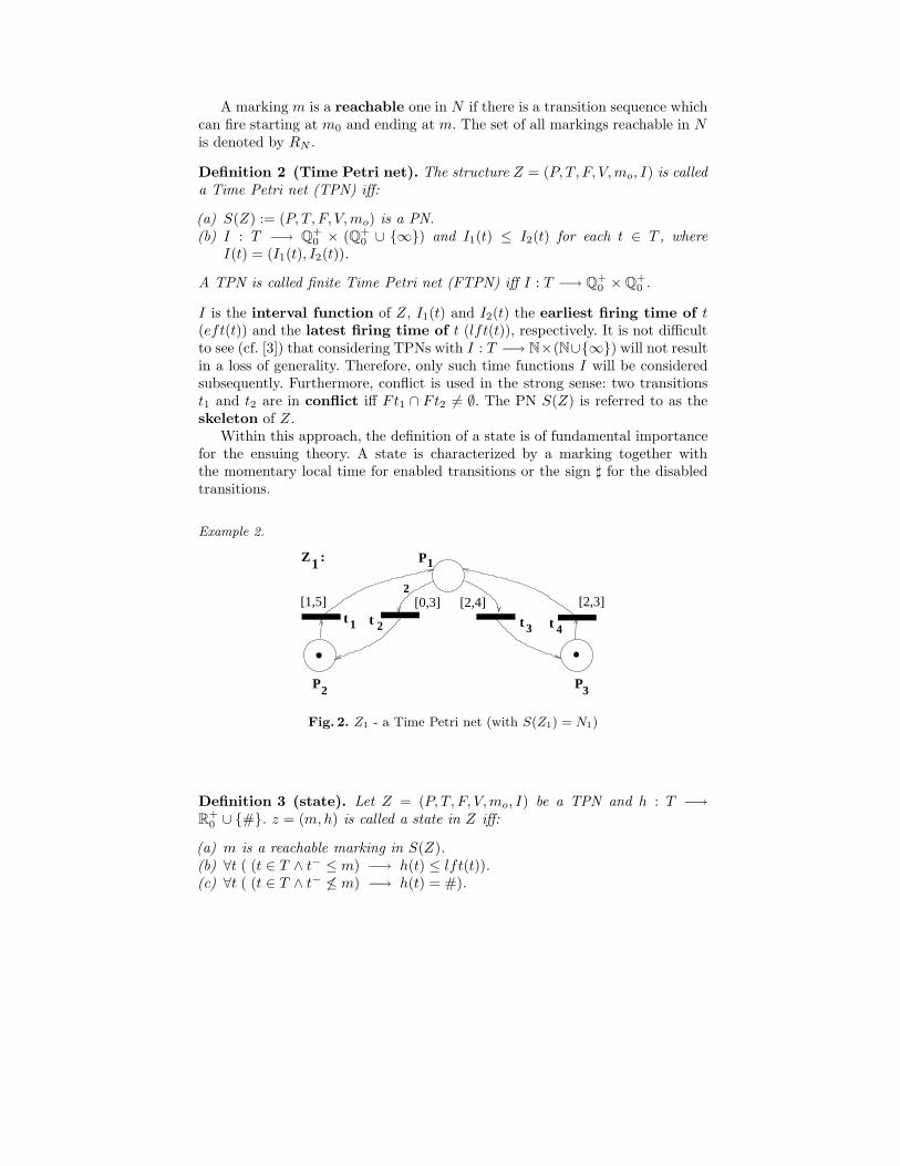
Fig. 2. Z1 - a Time Petri net (with S(Z1) = N1)

Definition 3 (state). Let Z = (P, T, F, V, mo, I) be a TPN and h : T −→R+

0 ∪ {#}. z = (m, h) is called a state in Z iff:

(a) m is a reachable marking in S(Z).(b) ∀t ( (t ∈ T ∧ t− ≤ m) −→ h(t) ≤ lft(t)).(c) ∀t ( (t ∈ T ∧ t− 6≤ m) −→ h(t) = #).

Interpretation of the notion “state” is as follows: within the net, each transitiont has a clock h(t). If t is enabled at a marking m, the clock of t h(t) showsthe time elapsed since t became most recently enabled. If t is disabled at m,the clock does not work (indicated by h(t) = #). Thus, the vector h which is avector of clocks is actually a transition marking and the already defined notion“marking” is in fact a place marking. In the following we call the places markingm a p-marking and the transitions marking h a t-marking.

The state zo := (mo, ho) with ho(t) :=

{0 iff t− ≤ m0

# iff t− 6≤ m0is set as the initial

state of the TPN Z.

Example 3.

The initial state in Z1 , compare Fig. 2, is z0 = ( (0, 1, 1)︸ ︷︷ ︸

p−marking

, (0, ], ], 0)︸ ︷︷ ︸

t−marking

).

Now the dynamic aspects of TPNs – changing from one state into another byfiring a transition or by time elapsing – can be introduced:

Definition 4 (state changing). Let Z = (P, T, F, V, mo, I) be a TPN, t be atransition in T and z = (m, h), z′ = (m′, h′) be two states. Then

(a) the transition t is ready to fire in the state z = (m, h), denoted by zt

−→ ,iff

(i) t− ≤ m and(ii) eft(t) ≤ h(t).

(b) the state z = (m, h) is changed into the state z′ = (m′, h′) by firing the

transition t, denoted by zt

−→ z′ , iff

(i) t is ready to fire in the state z = (m, h)(ii) m′ = m + ∆t and

(iii) ∀t ( t ∈ T −→ h′(t) :=

# iff t− 6≤ m′

h(t) iff t− ≤ m ∧ t− ≤ m′ ∧ Ft ∩ F t = ∅0 otherwise

).

(c) the state z = (m, h) is changed into the state z′ = (m′, h′) by the time

elapsing τ ∈ R+0 , denoted by z

τ−→ z′, iff

(i) m′ = m and(ii) ∀t ( t ∈ T ∧ h(t) 6= # −→ h(t) + τ ≤ lft(t) ) i.e. the time elapsing τ is

possible, and

(iii) ∀t ( t ∈ T −→ h′(t) :=

{h(t) + τ iff t− ≤ m′

# iff t− 6≤ m′ ).

The state z = (m, h) is called an integer state iff h(t) is an integer for eachenabled transition t in m.

Example 4.In the net Z1, in the initial state, the transitions t1 and t4 are enabled, but neithert1 nor t4 may fire because of their time restrictions. Thus, z0 can change into

another state only as time elapses. For example, the change of states z01.3−→ z1

is feasible, where z1 is given by m1 = m0 and h1 = (1.3, ], ], 1.3). Furthermore,

z1 can change into the state z2 with z11.0−→ z2, where the state z2 is given by

m2 = m1 and h2 = (2.3, ], ], 2.3). In z2 the transition t4 can fire, yielding thestate z3 with: m3 = (1, 1, 0) and h3 = (2.3, ], 0.0, ]). Now, as time progressesby 2, state z3 changes into the state z4, with m4 = m3, h4 = (4.3, ], 2.0, ]).Subsequently, t1 can fire and z4 is changed into a state z5 with m5 = (2, 0, 0)and h5 = (], 0.0, 2.0, ]). Afterwards t2 is ready to fire. Firing t2 at z5 leads toz6 = (m6, h6) with m6 = (0, 1, 0) and h6 = (0.0, ], ], ]). Thus, the sequence

zo1.3−→ z1

1.0−→ z2

t4−→ z32.0−→ z4

t1−→ z5t2−→ z6 is executable in Z1. The initial

state and the states z5 and z6 are integer states, whereas the states z1, z2, z3 andz4 are not.

Definition 5 (reachable state, state space). Let Z = (P, T, F, V, mo, I) bea TPN.

(a) The state z = (m, h) is called reachable in Z (starting at z0), iff there existstates z1, z

′1, ..., zn, z′n, transitions t1, ..., tn and times τi ∈ R+

0 , i = 1, ..., n

and it holds

z0τ1−→ z1

t1−→ z′1τ2−→ z2

t2−→ z′2...τn−→ zn

tn−→ z′n.

(b) The set StSp(Z) of all reachable states in Z is called the state space of Z.

It is easy to see that the set of all reachable p-markings in a TPN Z is the set{m | (m, h) ∈ StSp(Z)}, which will be denoted with RZ .

The sequence of transitions (t1, ..., tn) can fire in Z starting at z0, becausethere is a sequence (τ1, t1, ..., τn, tn). We denote such a transition sequenceσ = (t1, ..., tn) feasible. The sequence σ(τ) = (τ1, t1, ..., τn, tn) which is a con-crete execution of σ in Z is called a (feasible) run of σ. It is clear that in agiven TPN the state changes are achieved by alternating series of time elapsingand firing. Obviously, for a given run the transition sequence is well defined andfor a given transition sequence there are infinitely many runs in general.

It is clear that the state space of a TPN is in general infinite and densein terms of the time. On the one hand the set of reachable p-markings can beinfinite. On the other hand, for a fixed p-marking the set of t-markings can beinfinite. Nevertheless, it is possible to pick up some “essential” states only, sothat qualitative and quantitative analysis is possible. In [3] it is shown, that theessential states are the integer states.

The state space can be considered as the union of all sets Cσ, which aredefined below recursively:

Definition 6 (state class). Let Z = (P, T, F, V, mo, I) be a TPN and σ be afeasible transition sequence. The set Cσ is called a state class, iff

Basis: Ce := {z | ∃τ(τ ∈ R+0 ∧ z0

τ−→ z)}

Step: Let Cσ be already defined. Then Cσt is derived from Cσ by firing t

( denoted by Cσt

−→ Cσt ), iff

Cσt := {z | ∃z1∃z2∃τ(z1 ∈ Cσ ∧ τ ∈ R+0 ∧ z1

t−→ z2

τ−→ z)}.

In other words, the state class Ce is the set of all reachable states in Z that onegets after firing the empty transition sequence e at the initial state and afterwardsall states that are reachable by state changing with all possible elapses of time.That is why, sometimes C0 stands for Ce. Obviously, it holds StSp(Z) =

⋃

σ

Cσ.

3 Fundamental Property

The properties of a Petri net, both the classical one as well as the TPN, canbe divided into two parts: There are static properties, like being pure, ordinary,free choice, extended simple, conservative, etc., and there are dynamic propertieslike being bounded, live, reachable, and having place- or transitions invariants,deadlocks, etc. While it is easy to prove the static behavior of a net using only thestatic definition, the dynamic behavior depends on both the static and dynamicdefinitions and is quite complicated to prove. That means that in order to getgood knowledge of the dynamical behavior of the net, the set of all possiblesituations reachable for the net have to be known, i.e. the state space must beknown. As already mentioned, this set is in general infinite and therefore hardto handle.

Nevertheless, it is possible to pick up some “essential” states only, so thatqualitative and quantitative analysis is possible. In [3] it is shown, that theessential states are the integer-states.

The aim of this section is to justify the reduction of the state space of acertain TPN to a set of all its reachable integer-states as an adequate set fortesting dynamical properties. To do this we use dynamic programming.

Notions, notations, definitions and approach referring to dynamic programingare used similar to [5]. We consider the problem as a non-optimization problemjust like the abstract dynamic programming model considered in chapter 14.3 in[5] and solve it.

3.1 Parametric Description of the State Space

Let Z be an arbitrary TPN with the initial state z0 = (m0, h0). Let σ =(t1, ..., tn) be a feasible transition sequence in Z and let σ(τ) = (τ1, t1, ..., τn, tn)be a certain run. Obviously after firing σ(τ) a fix reachable state zσ(τ) is yielded.When the times τ = (τ1, ..., τn) are given parametrically with X = (x1, ..., xn)then the achieved state zσ(X) = (mσ(X), hσ(X)) is a parametrical one. It is easyto see that the p-marking mσ(X) does not depend on X . It depends only on σ.

However, the t-marking hσ(X) depends on σ as well as on the parameter X . Fur-thermore, it is clear that for a concrete value of X with the additional conditionthat the refering run is feasible, the t-marking hσ(X) is well defined. Hence, anunique parametric state zσ := zσ(X) can be assigned to each transition sequenceσ , i.e. we can consider a function between the set of all transition sequences inZ and the set of all reachable states, defined parametrically. In order to makecertain that σ is feasible we consider the parametric state zσ together with a setof conditions for the values of X . Thus, we can consider the state space as thecodomain of this function in connection with a set of certain additional condi-tions. It is clear that the codomain of this function is the parametric descriptionof the state space of the TPN.

In order to define and investigate this function it is convenient to transferthe subject matter into the terminology of a first-order predicate calculus. Ingeneral this terminology is used similar to [8]. Let Z be an TPN and let S :={f2, A2, $, ut, vt|t ∈ T } be a set of a symbols where f2 is a binary functionsymbol, A2 is a binary relation symbol, $ and ut, vt for each transition t areconstant symbols (for short: K := {$, ut, vt|t ∈ T } ). Furthermore, we considerthe S-structure D := [D, ω] with D := R+

0 ∪ {]} as a domain and

ω(f2) := +, ω(A2) :=≤, ω(ut) := eft(t), ω(vt) := lft(t), ω($) := ].

Here, + is a binary operation on D, which coincides with the well-known additionin R+

0 . In this context, it is not necessary to specify + any further. Similarconsiderations apply to ≤.

Let SUM be the union of the set of all terms, in which each variable ap-pears at most once and constants do not appear at all, and the set whichconsists only of the constant symbol $. COND denotes the set of all formu-lae A2termitermj where termi ∈ SUM \{$} and termj ∈ K \ {$}, or vice versa;the term in {termi, termj} ∩ (SUM \{$}) is denoted by s(A2termitermj), theone in {termi, termj}∩ (K \ {$}) with r(A2termitermj). Let β be an arbitraryassignment for the set of variables XS := {xi | i ∈ N} into the domain D. Underthe interpretation I := (D, β) , the value of a term with respect to β (which isan element in D) will be denoted by JtermKβ . In the following all used interpre-tations I = (D, β) consists of the same S-structure D, i.e. the interpretationsdiffer to each other in the assignment β only. Thus, the assertion ” β satisfy aformula c ” means that the interpretation I = (D, β) satisfy c.

Definition 1. Let Z = [P, T, F, V, m0, I] be a TPN. The function δ : T ∗ −→

RZ × SUM|T | ×℘(COND) is partially defined by induction:

Basis: δ(e) := [me, Σe, Be] where

(a) me = m0

(b) Σe(t) :=

{

x0 iff t− ≤ me

$ otherwise

(c) Be := {A2Σe(t)vt|t− ≤ me}.

Step: Let σ be a transition sequence and assume that δ(σ) has been definedas [mσ, Σσ, Bσ]. For a transition t with Σσ(t) 6= $, δ(σt) = [mσt, Σσt, Bσt] isdefined as follows:

(a) mσt := mσ + ∆(t),

(b) Σσt(t) :=

$ iff t− 6≤ mσt

xl(σ)+1 iff (t− 6≤ mσ ∧ t− ≤ mσt)∨

(t− ≤ mσ ∧ t− ≤ mσt ∧ Ft ∩ F t 6= ∅)

f2 Σσ(t)xl(σ)+1 otherwise

(c) Bσt := Bσt ∪ {A2utΣσ(t)} ∪ {A2Σσt(t)vt | t− ≤ mσt}

With regard to the interpretation of the symbols for functions, predicatesand constants in the logic defined above, the following notational conventionsfor terms in SUM \{$}, formulae in COND, and constants will be used for reasonsof convenience and increased readability:

x1 + · · · + xn := f2 . . . f2x1x2 . . . xn,

term1 ≤ term2 := A2term1term2,

and instead of constant symbols their interpretation under ω.

Obviously, there is a close connection between the state classes and the map-ping δ defined above: Cσ = {(mσ, Σσ(t)) | Bσ}.

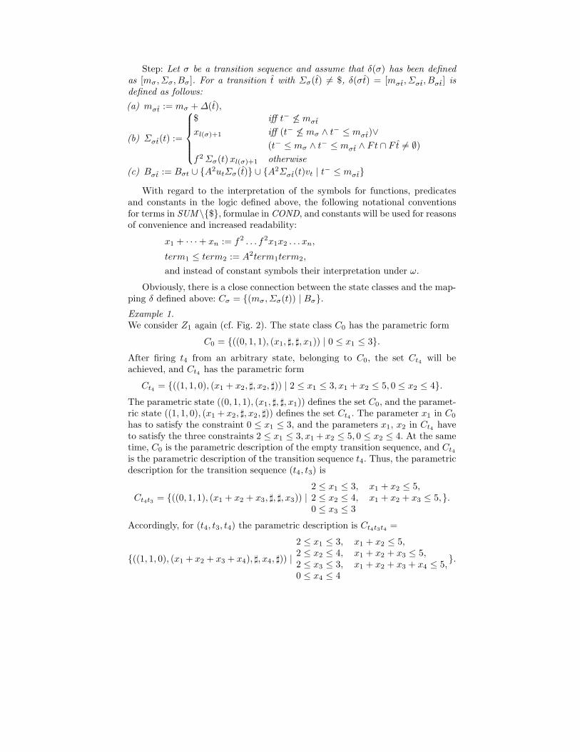
Example 1.We consider Z1 again (cf. Fig. 2). The state class C0 has the parametric form

C0 = {((0, 1, 1), (x1, ], ], x1)) | 0 ≤ x1 ≤ 3}.

After firing t4 from an arbitrary state, belonging to C0, the set Ct4 will beachieved, and Ct4 has the parametric form

Ct4 = {((1, 1, 0), (x1 + x2, ], x2, ])) | 2 ≤ x1 ≤ 3, x1 + x2 ≤ 5, 0 ≤ x2 ≤ 4}.

The parametric state ((0, 1, 1), (x1, ], ], x1)) defines the set C0, and the paramet-ric state ((1, 1, 0), (x1 + x2, ], x2, ])) defines the set Ct4 . The parameter x1 in C0

has to satisfy the constraint 0 ≤ x1 ≤ 3, and the parameters x1, x2 in Ct4 haveto satisfy the three constraints 2 ≤ x1 ≤ 3, x1 + x2 ≤ 5, 0 ≤ x2 ≤ 4. At the sametime, C0 is the parametric description of the empty transition sequence, and Ct4

is the parametric description of the transition sequence t4. Thus, the parametricdescription for the transition sequence (t4, t3) is

Ct4t3 = {((0, 1, 1), (x1 + x2 + x3, ], ], x3)) |2 ≤ x1 ≤ 3, x1 + x2 ≤ 5,

2 ≤ x2 ≤ 4, x1 + x2 + x3 ≤ 5,

0 ≤ x3 ≤ 3}.

Accordingly, for (t4, t3, t4) the parametric description is Ct4t3t4 =

{((1, 1, 0), (x1 + x2 + x3 + x4), ], x4, ])) |

2 ≤ x1 ≤ 3, x1 + x2 ≤ 5,

2 ≤ x2 ≤ 4, x1 + x2 + x3 ≤ 5,

2 ≤ x3 ≤ 3, x1 + x2 + x3 + x4 ≤ 5,

0 ≤ x4 ≤ 4

}.

3.2 Properties and Dynamic Programming

For each feasible transition sequence σ with δ(σ) = [mσ, Σσ, Bσ] it is easy toprove that the following holds:

Remark 1. For each state z ∈ Cσ, there is an assignment β : X −→ R+0 such

that: z = (mσ, JΣσKβ) and∧

b∈Bσ

β satisfies b.

Also easy to prove is the converse:

Remark 2. For each assignment β : X −→ R+0 with

∧

b∈Bσ

β satisfies b, the state

z := (mσ, JΣσKβ) is in Cσ.

By induction on σ it can be proved, too, that remark 3, remark 4 and remark5 are true:

Remark 3. For any two transitions ti and tj in Z with Σσ(ti) = xi0+xi1+· · ·+xik

and Σσ(tj) = xj0 + xj1 + · · · + xjl, it follows that ik−r = jl−r for all r =

0, 1, . . . , min{k, l}.

Remark 4. For each transition t ∈ T it is true that: if Σσ(t) = xi + . . .+xj theneach variable xk with i ≤ k ≤ j also appears in Σσ(t).

Remark 5. For each term ∈ SUM , which is a part of a formula b in Bσ, it istrue that: if term = xi + . . . + xj then each variable xk with i ≤ k ≤ j alsoappears in term.

The following theorem supplies the fundamental property of the TPN thatallows one to consider an essential reduced state space.

Theorem 1. Let Z = [P, T, F, V, m0, I] be a TPN, σ a transition sequence of

length n, with δ(σ) = [mσ, Σσ, Bσ] and β : X −→ R+0 an assignment such that

∀c(c ∈ Bσ → β satisfies c). Then there exists an assignment β∗ : X −→ N suchthat:

(1) ∀c(c ∈ Bσ → β∗ satisfies c)(2) ∀t(t ∈ T ∧ t− ≤ mσ → JΣσ(t)Kβ∗ ≤ JΣσ(t)K

β)

(3)q n∑

k=0

xk

yβ∗

≤q n∑

k=0

xk

yβ.

The meaning of the theorem is that if β supplies a feasible run for σ withreal numbers for elapsed time then it is possible to find a further feasible runfor σ with integer time elapses (meaning of (1)). The differences between therespective time elapses in both runs are allways smaller than 1 (follows fromthe construction of β∗ given below). The difference between the clocks of eachenabled transition at mσ after the first run and after the second one is smaller

than 1, too ( meaning of (2)). And finally also the difference between the totaltimes of both runs is smaller than 1 (meaning of (3)).

Idea of the proof: The integer values β∗(x1), β∗(x2), · · · , β∗(xn) defined by

the assignment β∗ will be explicitly constructed out of the given assignment β

by successively transforming each non-integral real number to the nearby integerin (n + 1) steps.

As the default value brc will be taken, in order to ensure that the second andthird property stated in the theorem are satisfied. By doing so, the restrictionyielded by the first property will be somewhat loosened, i.e., temporarily it issufficient that a required condition is “almost” satisfied. This means, that foreach formula c in Bσ, the value of the non-constant term s(c) under the currentassignment will only have to lie in a certain neighbourhood of the initial valueJs(c)K

β.

If, by taking the integer part of the rational value for a certain variable, sucha neighbourhood will be left for at least one condition, dre will be taken instead.The largest part of the proof aims to show that the three requirements statedabove will also be satisfied (with the first one once again “loosened”) in thiscase.

To complete the proof, it then remains to verify, that for the finally con-structed assignment, which takes only integer values, the “loosened” version ofthe first requirement is equivalent to the original one.

Construction of β∗

Let Xσ be the set of all variables which appear in Bσ, i.e. Xσ := {x0, x1, . . . , xn}define a finite sequence of assignments βi : Xσ −→ R+

0 by induction:

Basis: β0 : Xσ −→ R+0 with β0(x) := β(x) for all x ∈ Xσ.

Step: Assume that βi−1 has been defined. In order to describe the construc-tion of βi, the following function is used:

βi(x) :=

{

βi−1(x) iff x 6= xn−(i−1)

bβi−1(x)c otherwise

Now define βi : Xσ −→ R+0 by

βi(x) :=

βi−1(x) iff x 6= xn−i+1

bβi−1(x)c iff x = xn−i+1 ∧ ∀c(c ∈ Bσ → bJs(c)Kβ0c − 1 < Js(c)Kβi

)

dβi−1(x)e otherwise

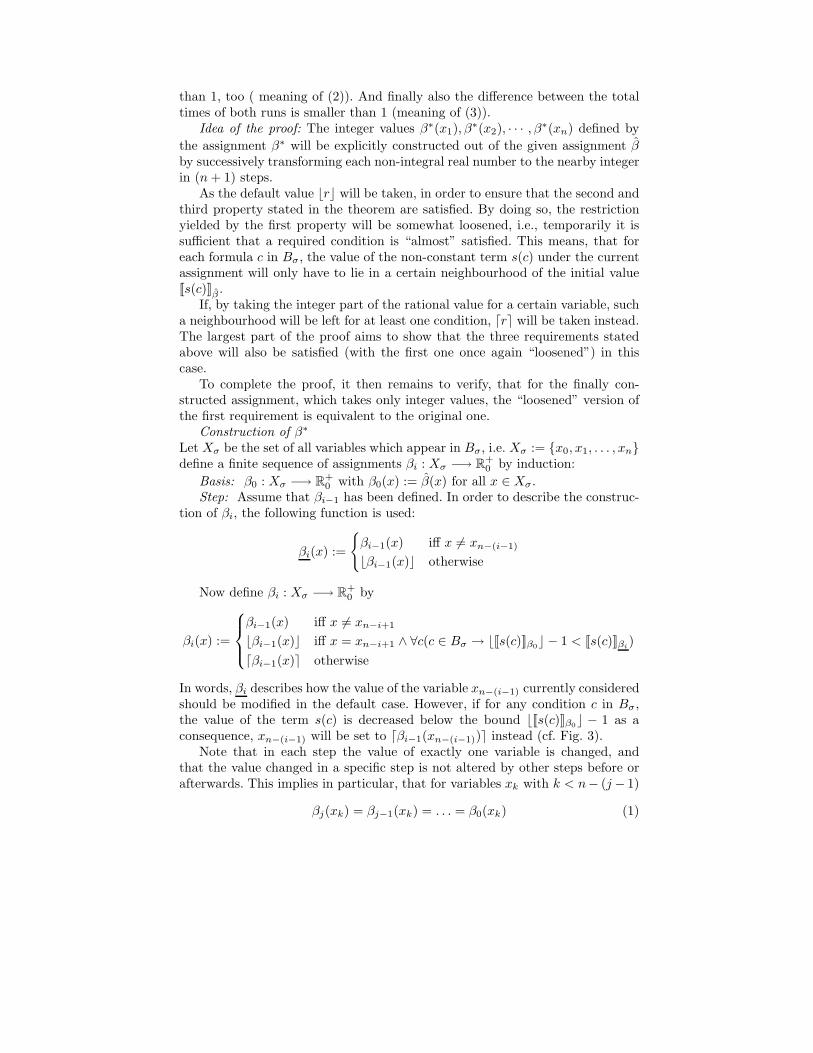
In words, βi describes how the value of the variable xn−(i−1) currently consideredshould be modified in the default case. However, if for any condition c in Bσ,the value of the term s(c) is decreased below the bound bJs(c)Kβ0

c − 1 as aconsequence, xn−(i−1) will be set to dβi−1(xn−(i−1))e instead (cf. Fig. 3).

Note that in each step the value of exactly one variable is changed, andthat the value changed in a specific step is not altered by other steps before orafterwards. This implies in particular, that for variables xk with k < n− (j − 1)

βj(xk) = βj−1(xk) = . . . = β0(xk) (1)

e

bJs(c)Kβ0c − 1 dJs(c)Kβ0

e + 1

dJs(c)Kβ0ebJs(c)Kβ0

c

Js(c)Kβ0

Fig. 3. Position of the real number Js(c)Kβ0and the integers bJs(c)Kβ0

c− 1, bJs(c)Kβ0c,

dJs(c)Kβ0e and dJs(c)Kβ0

e + 1

and that for variables xk with k ≥ n − (j − 1)

βj(xk) = βj+1(xk) = . . . = βn+1(xk) (2)

Furthermore, if β0(xn−(i−1)) is already an integer, then βi leaves xn−(i−1) unal-tered, since for any integer k, k = bkc = dke.

Obviously all values βn+1(x0), βn+1(x1), . . . , βn+1(xn) are integers. Thus

β∗(xj) := βn+1(xj) for each j = 0, 1, . . . , n.

The ensuing tableau points up the successive constructing of β∗ from β:

β β(x0) β(x1) · · · β(xn−j) β(xn−(j−1)) · · · β(xn−1) β(xn)

β := β0 r r · · · r r · · · r r

β1 r r · · · r r · · · r i

β2 r r · · · r r · · · i i...

......

βj r r · · · r i · · · i i...

......

βn r i · · · i i · · · i i

β∗ := βn+1 i i · · · i i · · · i i

The r in the tableau above stands for (nonnegative) real number and i – for(nonnegative) integer.

The following three assertions about this sequence of assignments bundled inthe next lemma are proved by induction for each i:

Lemma 1. For all i ∈ {0, 1, . . . , n + 1} it holds:

(a) ∀c(c ∈ Bσ → Js(c)Kβi∈ ( bJs(c)Kβ0

c − 1, dJs(c)Kβ0e + 1 ) )

(b) ∀t(t ∈ T ∧ t− ≤ mσ → JΣσ(t)Kβi≤ JΣσ(t)Kβ0

)

(c)q n∑

k=0

xk

yβi

≤q n∑

k=0

xk

yβ0

Before starting the proof please note that (a), (b) and (c) from lemma 1supply a finite number of inequalities. Namely (a) derives from each inequalityof V C1 two further inequalities:

Js(c)Kβi≥ bJs(c)Kβ0

c − 1 and

Js(c)Kβi≤ dJs(c)Kβ0

e + 1,

(b) supplies at most as many inequalities as the number of transitions in theTPN and (c) delivers one inequality.

And as a last discussion before starting the proofs let us consider the asser-tion of the theorem 1 more precisely and elaborate the connection to dynamicprogramming. The theorem 1 solves the following problem :

Input: a TPN, a transition sequence σ = (t1, . . . , tn) anda sequence of (n + 1) real numbers,

(β(x0), β(x1), · · · , β(xn)) subject to a certain finiteset V C1 of conditions.

Output: a sequence of (n + 1) integers,(β∗(x0), β

∗(x1), · · · , β∗(xn)) subject to V C.

Thus, let now consider the solving of the output as the problem P∗, thatmeans:

Problem P∗: Compute a sequence of (n + 1) integers,(β∗(x0), β

∗(x1), · · · , β∗(xn)) subject to V C∗2.

The solution strategy for the problem P∗ is a typical dynamic programming’sone:

In the following disquisition about the connection between solving the prob-lem P∗ and dynamic programming (DP) we use certain notions and notationstypical for both the theory of DP, and the theory of TPN. However, the meaningsof the notions state, state space, transition function etc. are different betweenthe two theories. The meaning of these should however be clear from the context.Once again, DP notions and notations used here are the same as those in [5].

Thus, the target problem, now is Problem P∗.The set of solutions of this problem zo is set of all sequences of integers

(β∗(x0), β∗(x1), · · · , β∗(xn)) subject to V C.

1 V C is derived from the set of formulae Bσ where relation- and function symbols areinterpreted, i.e. V C is a finite set of inequalities with the variables x0, x1, . . . , xn.Thus (β(x0), β(x1), · · · , β(xn)) subject to the finite set V C means that the realnumbers β(x0), β(x1), · · · , β(xn) satisfy all inequalities of V C. The semantics of thisis that the run σ(β) = (β(x0), t1, β(x1), t2, · · · , tn, β(xn) ) is a feasible one in theTPN.

2 V C∗ is the union of the set V C and the finite set of inequalities supply by (a), (b)and (c). The semantics of this is that if the run σ(β) is feasible one in the TPN,than the run σ(β∗) is feasible in the TPN, too, and the set of all transitions whichare ready to fire after the run σ(β∗) is the same as the set of all transitions whichare ready to fire after the run σ(β).

The state space (for P∗) is the set S = {0, 1, . . . , n}.The family of the modified problems P∗(s), s∈S are obviously the problems

Problem P∗(s): Compute a sequence of (n + 1) numbers,(βs(x0), β

s(x1), · · · , βs(xn) withβs(x0), β

s(x1), · · · , βs(xn−s)) are reals andβs(xn−(s−1)), · · · , βs(xn) are integerssubject to V C∗.

The existence of the assignment βs for each s is verified by lemma 1.

The set of its critical states is the singleton So = {n}.

The set of its terminal states is the singleton St = {0}.

Thus the set of non-terminal states is S′′ = S \ St = {1, 2, . . . , n}.The T-linker LT has the form LT(z(so)) = zo = z(so).The transition function t is defined as

t(s) := s - 1, s ∈ S′′.

And lastly the linker L is clearly given by

z(s) = L(s, {(s′,z(s′)) | s′ ∈ t(s)}), ∀s ∈ S′′

= L(s, z(t(s)))

= L(s,z(s-1)) := βs

and βs is defined as in the constuction of β∗.

Now we are going to verify Lemma 1. The subsequent example 3.1 illustratesthe use of DP for a concrete TPN.

Proof of Lemma 1:Induction on i:Basis: For i = 0, all three assertions are trivially true.Step: Assume that the assertions have been justified for each of 1, . . . , i, and

consider the case i + 1. If βi(xn−i) ∈ N, then βi+1 = βi and all assertions followimmediately from the induction hypothesis. Therefore, it may be assumed thatβi(xn−i) is not an integer.

Two cases need to be considered:

Case 1: βi+1(xn−i) = bβi(xn−i)cHence, it holds:

βi+1(x) ≤ βi(x) for each x ∈ Xσ. (3)

to (a):Let b be any condition (i.e. a formula) in Bσ. If xn−i does not appear in s(b),then Js(b)Kβi+1

= Js(b)Kβi, and the first assertion follows from the induction

hypothesis. Hence, assume that xn−i is in s(b).

Since βi+1(x) ≤ βi(x) for each x ∈ Xσ, it is evident that

Js(b)Kβi+1≤ Js(b)Kβi

By the induction hypothesis, Js(b)Kβi< dJs(b)Kβ0

e + 1, so the previous in-equality becomes

Js(b)Kβi+1< dJs(b)Kβ0

e + 1 (4)

As βi+1(xn−i) has been set to bβi(xn−i)c, the corresponding criteria in thedefinition of βi+1

∀c(c ∈ Bσ → bJs(c)Kβ0c − 1 < Js(c)Kβi+1

)

has been fulfilled. Since βi+1 = βi+1, it follows for the condition b in partic-ular:

bJs(b)Kβ0c − 1 < Js(b)Kβi+1

(5)

Because b was chosen arbitrarily, the inequalities (4) and (5) combine provethe first assertion in the case i + 1, and therefore complete the inductionstep.to (b):The inequality (3) leads immediately to

JΣσ(t)Kβi+1≤ JΣσ(t)Kβi

for each transition t which is enabled after the firing of σ, and because ofthe induction hypothesis

JΣσ(t)Kβi≤ JΣσ(t)Kβ0

the second assertion (b) is proved.to (c):The inequality (3) instantaneously yields (c).

Case 2: βi+1(xn−i) = dβi(xn−i)ei.e. a formula c exists in Bσ, such that

Js(c)Kβi+1≤ bJs(c)Kβ0

c − 1 (6)

and thus xn−i does appear in c.Further it is true in this case that:

βi(x) ≤ βi+1(x) for each x ∈ Xσ. (7)

to (a):Let b be any formula in Bσ again. Then it holds:

bJs(b)Kβ0c − 1 < Js(b)Kβi

ind. hypothesis

≤ Js(b)Kβi+1because of (7) (8)

On the other hand, it is true for the formula c:

Js(c)Kβi+1= Js(c)Kβi

− βi(xn−i) + βi+1(xn−i)

= Js(c)Kβi− βi(xn−i) + dβi(xn−i)e

= Js(c)Kβi− βi(xn−i) + bβi(xn−i)c + 1

= Js(c)Kβi+1+ 1

≤ bJs(c)Kβ0c because of (6)

i.e.

Js(c)Kβi+1≤ bJs(c)Kβ0

c (9)

and therefore Js(c)Kβi+1≤ Js(c)Kβ0

is true, too. (10)

Because of (8) and (9) assertion (a) holds for the formula c.Now suppose that

Js(b)Kβi+1≥ dJs(b)Kβ0

e + 1 (11)

which in particular implies

Js(b)Kβi+1≥ Js(b)Kβ0

+ 1. (12)

Let jc and kc be the minimal and maximal variable index which appears ins(c), respectively. Refering to Remark 5. above it is clear that

s(c) = xjc+ xjc+1 + . . . + xn−i + xn−(i−1) + . . . + xkc

. (13)

Similarly, there are indices jb and kb such that

s(b) = xjb+ xjb+1 + . . . + xn−i + xn−(i−1) + . . . + xkb

. (14)

Hence, it holds for the indices n − i, kc and kb:

n − i ≤ kc and n − i ≤ kb

i.e. n − kc < i + 1 and n − kb < i + 1

The values of the variables according to the two assignments β0 and βi+1

are:

βi+1(xjc) · · · βi+1(xn−(i+1))

︸ ︷︷ ︸

βi+1 = β0

↑ ↑real real

βi+1(xn−i) · · · βi+1(xkc)

︸ ︷︷ ︸

βi+1 6= β0

↑ ↑int. real

(15)

According to the definition (construction) of β∗ it is clear, that the assign-ment βi+1 changes the value of the variable xn−i and the assignment βn−r

changes the value of xr+1.Hence, refering to (13), (10) may be rewritten as

(βi+1(xjc) − β0(xjc

))+

(βi+1(xjc+1) − β0(xjc+1)) + . . .+

(βi+1(xn−i) − β0(xn−i)) + (βi+1(xn−i+1) − β0(xn−i+1)) + . . .+

(βi+1(xkc) − β0(xkc

)) ≤ 0

(16)

and refering to (15), (16) may be rewritten as

(βi+1(xn−i) − β0(xn−i) + (βi+1(xn−i+1) − β0(xn−i+1)) + . . .+

(βi+1(xkc) − β0(xkc

)) ≤ 0(17)

Similarly, (12) and (14) yield

(βi+1(xn−i) − β0(xn−i)) + (βi+1(xn−i+1) − β0(xn−i+1)) + . . .+

(βi+1(xkb) − β0(xkb

)) ≥ 1(18)

Three sub-cases need to be considered:

Case 2.1: kc = kb

Then it holds:

1 ≤ Js(b)Kβi+1− Js(b)Kβ0

because of (12)

= Js(c)Kβi+1− Js(c)Kβ0

because of (17) and 18

≤ 0 because of (10)

Clearly, this is a contradiction.

Case 2.2: kc < kb

In this case the two terms s(c) and s(b) have the form:

s(c) = xjc+ · · · +xn−i+ · · · + xkc

s(b) = xjb+ · · · +xn−i+ · · · + xkc

+ · · · + xkb

Because of (1) and (2) this leads to the following values of the variablesin s(b) according to the assignments β0, βn−kc

and βn+1 :

s(b) =

β0=βn−kc

︷ ︸︸ ︷

xjb+ · · ·+

︸ ︷︷ ︸

βi+1 = βn−kc

↑ ↑real real

xn−i + · · · + xkc︸ ︷︷ ︸

βi+1 6= βn−kc

↑ ↑int. real

β0 6=βn−kc

︷ ︸︸ ︷

+ · · · + xkb︸ ︷︷ ︸

βi+1 = βn−kc

↑ ↑int. int.

. (19)

Now consider the values of the term s(b) according to the assignmentsβi+1 and βn−kc

.

Because of (19), βo and βn−kcagree on all variables with indices not

greater then kc. That is way inequality (17) leads to

(βi+1(xn−i) − βn−kc(xn−i)+

(βi+1(xn−i+1) − βn−kc(xn−i+1)) + . . . +

(βi+1(xkc) − βn−kc

(xkc)) ≤ 0

(20)

Thus (19) and (20) yield

Js(b)Kβi+1− Js(b)Kβn−kc

≤ 0 (21)

But (11) and (21) then yield

Js(b)Kβn−kc≥ dJs(b)Kβ0

e + 1

which contradicts the induction hypothesis for n−kc, then n−kc < i+1.Case 2.3: kc > kb

Now the two terms s(c) and s(b) have the form:

s(c) = xjc+ · · · +xn−i+ · · · + xkb

+ · · · xkc

s(b) = xjb+ · · · +xn−i+ · · · + xkb

Analogosly to Case 2.2 this leads to the following values of the variablesin s(b) according to the assignments β0, βn−kb

and βn+1 :

s(c) =

β0=βn−kb

︷ ︸︸ ︷

xjb+ · · · +

︸ ︷︷ ︸

βi+1 = βn−kb

↑ ↑real real

xn−i + · · · + xkb︸ ︷︷ ︸

βi+1 6= βn−kb

↑ ↑int. real

β0 6=βn−kb

︷ ︸︸ ︷

+ · · · + xkc︸ ︷︷ ︸

βi+1 = βn−kb

↑ ↑int. int.

. (22)

Now the term s(c) will be evaluated by the assignments βi+1 and βn−kb

and afterwards Js(b)Kβi+1and Js(b)Kβn−k

bwill be compared:

Because of (22), βi+1 and βn−kbagree on all variables with indices smaller

than n − i and also agree on all variables with indices greater than kb.That is why the inequality (18) leads to

(βi+1(xn−i) − βn−kb(xn−i)+

(βi+1(xn−i+1) − βn−kb(xn−i+1)) + . . . +

(βi+1(xkb) − βn−kb

(xkb)) ≥ 1

(23)

Hence, (23) together with (13) show that

Js(c)Kβi+1− Js(c)Kβn−k

b≥ 1 (24)

But (9) and (24) then yield

Js(c)Kβn−kb≤ bJs(c)Kβ0

c − 1

which contradicts the induction hypothesis for n−kb, then n−kb < i+1.

The assumption (11) has led to a contradiction in all three sub-cases. There-fore the following inequality must hold:

Js(b)Kβi+1< dJs(b)Kβ0

e + 1 (25)

Because b was chosen arbitrarily, (8) and (25) prove the first assertion (a).

to (b):Let t be a transition which is not disabled after the firing of σ. If xn−i does

not appear in Σσ(t), then JΣσ(t)Kβi+1= JΣσ(t)Kβi

, and JΣσ(t)Kβi+1≤ JΣσ(t)Kβ0

follows from the induction hypothesis. Therefore, assume that xn−i does appearin Σσ(t).

By the construction of Σσ (cf. remark 3), xn appears in every componentwhich is not $. Referring to remark 4, this implies that there is an index jt suchthat

Σσ(t) = xjt+ xjt+1 + . . . + xn−i + xn−(i−1) + . . . + xn (26)

Because of (19), βi+1 and βn−kcagree on all variables with indices smaller

than n − i and on all variables with indices greater than kc.Hence, (20) together with (26) show that

JΣσ(t)Kβi+1− JΣσ(t)Kβn−kc

≤ 0 (27)

Using the induction hypothesis for n − kc, (27) yields

JΣσ(t)Kβi+1≤ JΣσ(t)Kβ0

Since t was chosen arbitrarily, the second assertion (b) is also proved.to (c):Again, because of (19), βi+1 and βn−kc

agree on all variables with indicessmaller than n − i and on all variables with indices greater than kc it followsfrom (20):

q n∑

k=0

xn

yβi+1

≤q n∑

k=0

xn

yβn−kc

But by the induction hypothesis for n − kc,

q n∑

k=0

xn

yβn−kc

≤q n∑

k=0

xn

yβ0

which, together with the previous inequality, proves the third assertion (c):

q n∑

k=0

xn

yβi+1

<q n∑

k=0

xn

yβ0

.

With it the lemma 1 is proved. �

Proof of theorem 1:It is obvious, that (a), (b) and (c) lead to the validation of the assertions of

the theorem 1: It is immediately clear, that property (2) is the same as (b) andresp. (3) is the same as (c) for setting β∗ := βn+1 .

Consider a condition c in Bσ. Since β∗ assigns only integers to the variables,Js(c)Kβ∗ is also an integer. The first assertion in lemma 1 implies that

Js(c)Kβ∗ ∈ (bJs(c)Kβ0c − 1, dJs(c)Kβ0

e + 1)

But the only integers in the interval (bJs(c)Kβ0c−1, dJs(c)Kβ0

e+1) are bJs(c)Kβ0c

and dJs(c)Kβ0e.

r(c) is a constant symbol, which is interpreted by ω as an integer, namelyeft(t) or lft(t) for some transition t. Clearly, if for a given real number r and aninteger i, the inequalities r ≤ i or i ≤ r hold, then brc ≤ i or i ≤ brc are alsofulfilled, respectively, and the same applies to dre.

Therefore, for both possible values bJs(c)Kβ0c and dJs(c)Kβ0

e of Js(c)Kβ∗ , itfollows that β∗ satisfies c.

Since c was chosen arbitrarily, β∗ satisfies all conditions in Bσ, so that prop-erty (1) stated in the theorem follows from lemma 1(a) and hence theorem 1 isproved. �

The next proposition immediately follows from theorem 1:

Corollary 1. Let z = (m, h) be an arbitrary reachable state in a TPN Z. Thenthe state z := (m, bhc) is also reachable in Z.

Proof: The existence of z := (m, bhc) follows immediately from theorem 1(2).�

The next theorem can be proved analogously to theorem 1.

Theorem 2. Let Z = [P, T, F, V, m0, I] be a TPN, σ a transition sequence of

length n, with δ(σ) = [mσ, Σσ, Bσ] and β : X −→ R+0 an assignment such that

∀c(c ∈ Bσ → β satisfies c). Then there exists an assignment β∗ : X −→ N suchthat:

(a) ∀c(c ∈ Bσ → β∗ satisfies c)(b) ∀t(t ∈ T ∧ t− ≤ mσ → JΣσ(t)Kβ∗ ≥ JΣσ(t)K

β)

(c)q n∑

k=0

xk

yβ∗

≥q n∑

k=0

xk

yβ

Corollary 2. Let z = (m, h) be an arbitrary reachable state in a TPN Z. Thenthe state z := (m, dhe) is also reachable in Z.

Proof: The existence of z := (m, dhe) follows immediately from theorem 2(2).�

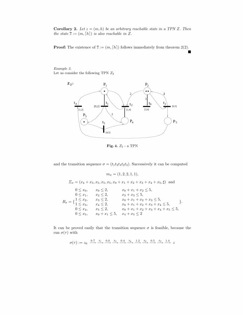
Example 2.

Let us consider the following TPN Z2

[1,2]

[4,5]

[1,4] [3,6][0,5]

t[0,2]

t t t

P

P1

3

P2

5

P

P4

3

t

t2 64 1

5

2

2

3

22

Z :2

Fig. 4. Z2 - a TPN

and the transition sequence σ = (t1t3t4t2t3). Successively it can be computed

mσ = (1, 2, 2, 1, 1),

Σσ = (x4 + x5, x5, x5, x5, x0 + x1 + x2 + x3 + x4 + x5, ]) and

Bσ = {

0 ≤ x0, x0 ≤ 2, x0 + x1 + x2 ≤ 5,

0 ≤ x1, x2 ≤ 2, x2 + x3 ≤ 5,

1 ≤ x2, x3 ≤ 2, x0 + x1 + x2 + x3 ≤ 5,

1 ≤ x3, x4 ≤ 2, x0 + x1 + x2 + x3 + x4 ≤ 5,

0 ≤ x4, x5 ≤ 2, x0 + x1 + x2 + x3 + x4 + x5 ≤ 5,

0 ≤ x5, x0 + x1 ≤ 5, x4 + x5 ≤ 2

}.

It can be proved easily that the transition sequence σ is feasible, because therun σ(τ) with

σ(τ) := z00.7−→

t1−→0.0−→

t3−→0.4−→

t4−→1.2−→

t2−→0.5−→

t3−→1.4−→ z

is a feasible one in Z2. This is the case, since the values 0.7, 0.0, 0.4, 1.2, 0.5,

1.4 assign to the variables x1, x2, x3, x4, x5 (with an assignment β) satisfy Bσ.

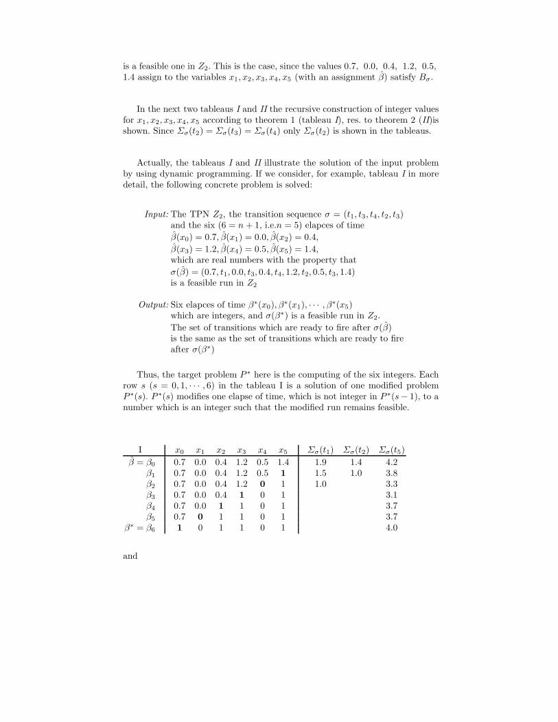
In the next two tableaus I and II the recursive construction of integer valuesfor x1, x2, x3, x4, x5 according to theorem 1 (tableau I), res. to theorem 2 (II)isshown. Since Σσ(t2) = Σσ(t3) = Σσ(t4) only Σσ(t2) is shown in the tableaus.

Actually, the tableaus I and II illustrate the solution of the input problemby using dynamic programming. If we consider, for example, tableau I in moredetail, the following concrete problem is solved:

Input: The TPN Z2, the transition sequence σ = (t1, t3, t4, t2, t3)and the six (6 = n + 1, i.e.n = 5) elapces of time

β(x0) = 0.7, β(x1) = 0.0, β(x2) = 0.4,

β(x3) = 1.2, β(x4) = 0.5, β(x5) = 1.4,which are real numbers with the property that

σ(β) = (0.7, t1, 0.0, t3, 0.4, t4, 1.2, t2, 0.5, t3, 1.4)is a feasible run in Z2

Output: Six elapces of time β∗(x0), β∗(x1), · · · , β∗(x5)

which are integers, and σ(β∗) is a feasible run in Z2.

The set of transitions which are ready to fire after σ(β)is the same as the set of transitions which are ready to fireafter σ(β∗)

Thus, the target problem P ∗ here is the computing of the six integers. Eachrow s (s = 0, 1, · · · , 6) in the tableau I is a solution of one modified problemP ∗(s). P ∗(s) modifies one elapse of time, which is not integer in P ∗(s− 1), to anumber which is an integer such that the modified run remains feasible.

I x0 x1 x2 x3 x4 x5 Σσ(t1) Σσ(t2) Σσ(t5)

β = β0 0.7 0.0 0.4 1.2 0.5 1.4 1.9 1.4 4.2β1 0.7 0.0 0.4 1.2 0.5 1 1.5 1.0 3.8β2 0.7 0.0 0.4 1.2 0 1 1.0 3.3β3 0.7 0.0 0.4 1 0 1 3.1β4 0.7 0.0 1 1 0 1 3.7β5 0.7 0 1 1 0 1 3.7

β∗ = β6 1 0 1 1 0 1 4.0

and

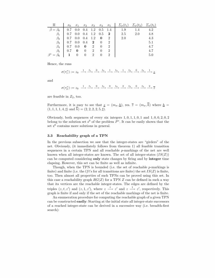
II x0 x1 x2 x3 x4 x5 Σσ(t1) Σσ(t2) Σσ(t5)

β = β0 0.7 0.0 0.4 1.2 0.5 1.4 1.9 1.4 4.2β1 0.7 0.0 0.4 1.2 0.5 2 2.5 2.0 4.8β2 0.7 0.0 0.4 1.2 0 2 2.0 4.3β3 0.7 0.0 0.4 2 0 2 5.1β4 0.7 0.0 0 2 0 2 4.7β5 0.7 0 0 2 0 2 4.7

β∗ = β6 1 0 0 2 0 2 5.0

Hence, the runs

σ(τ∗1 ) := z0

1−→

t1−→0

−→t3−→

1−→

t4−→1

−→t2−→

0−→

t3−→1

−→ z

and

σ(τ∗2 ) := z0

1−→

t1−→0

−→t3−→

0−→

t4−→2

−→t2−→

0−→

t3−→2

−→ z

are feasible in Z2, too.

Furthermore, it is easy to see that z = (mσ, h), res. z = (mσ, h) where h =(1, 1, 1, 1, 4, ]) and h) = (2, 2, 2, 2, 5, ]).

Obviously, both sequences of every six integers 1, 0, 1, 1, 0, 1 and 1, 0, 0, 2, 0, 2belong to the solution set z0 of the problem P ∗. It can be easily shown that theset z0 contains more solutions in general.

3.3 Reachability graph of a TPN

In the previous subsection we saw that the integer-states are “girders” of thenet. Obviously, (it immediately follows from theorem 1) all feasible transitionsequences in a certain TPN and all reachable p-markings of the net are wellknown when all integer-states are known. The set of all integer-states (IS(Z))can be computed considering only state changes by firing and by integer timeelapsing. However, this set can be finite as well as infinite.

Though, when the TPN is bounded (i.e. the set of reachable p-markings isfinite) and finite (i.e. the lft’s for all transitions are finite) the set IS(Z) is finite,too. Then almost all properties of such TPNs can be proved using this set. Inthis case a reachability graph RG(Z) for a TPN Z can be defined in such a waythat its vertices are the reachable integer-states. The edges are defined by the

triples (z, t, z′) and (z, 1, z′), where zt

−→ z′ and z1

−→ z′, respectively. Thisgraph is finite if and only if the set of the reachable markings of the net is finite.

An enumeration procedure for computing the reachable graph of a given TPNcan be constructed easily: Starting at the initial state all integer-state successorsof a reached integer-state can be derived in a successive way (i.e. breadth-firstsearch):

Basis)z0 ∈ RG(Z)

Step)Let z be in RG(Z) already.1. for i=1 to n do

if zti−→ z′ possible in Z (cf. def 4) then z′ ∈ RG(Z) end

2. if z1

−→ z′ possible in Z (cf. def 4) then z′ ∈ RG(Z)

The reachability graph defined above can be reduced: 1st stage – all verticesthat have input and output edges labeled with time only can be ignored. Theirinput edges are merged with their output edges (each input edge with eachoutput one) and labeled with the sum of both labels. A further reduction canbe accomplished as follow: 2nd stage – all vertices which have input edges withtime only can be ignored, too. Their input edges are merged with their outputedges labeled with the both labels (from the input and from the output edges).However the second reduction decreases the number of vertices but the labels ofthe merged edges are more complex then the remained labels. For more see e.g.[2] or [9]. From now on we are going to use the notion reachability graph in thesense of (double) reduced reachability graph.

Unfortunately, the reachability graph defined above is not finite if there is atransition t with lft(t) = ∞, even though the net is bounded. Nonetheless, thetime after reaching the eft(t) is not important for t actually. Thus, when theclock h(t) reaches the eft, i.e. h(t) = eft(t) than it is not necessary to incrementthe time for this transition anymore (even though the time is going on). That iswhy we modify the definition 4(c)(iii) as follows:

(iii)′ ∀t ( t ∈ T −→ h′(t) :=

h(t) + τ iff t− ≤ m′ ∧ eft(t) ≥ h(t) + τ

eft(t) iff t− ≤ m′ ∧ eft(t) < h(t) + τ

# iff t− 6≤ m′).

It can be proved by induction that in a TPN a transition sequence is feasibleaccording to definition 4(c)(iii) if and only if it is feasible according to definition4′. The crucial advantage of the modified reachable graph which is obtained byusing the modified definition 4′ is the property from above: it is finite if and onlyif the TPN is bounded.

Furthermore, it is easy to see that in the case of a finite TPN both definitionsdeliver the same set of reachable integer-states, i.e. the modified definition 4′ isa consistent extension of definition 4 if the class of considered TPNs is extended.

The enumeration procedure for computing the reachable graph of a givenTPN defined above can be performed using the modified definition 4′. The resultis the modified reachability graph. This graph can be reduced in the same manneras RG(Z), too.

Example 3.

Let us consider the finite TPN Z2. The full reachability graph RG(1)(Z2) aswell as the reduced reachability graphs RG(2)(Z2) (1st stage of reduction) andRG(Z2) (2nd stage of reduction) are illustrated below:

[0,1]

[0,1]

[2,3]

t1

t

t

2

3

P

P

1 P

P3

2

4

Z :2

z zz0

z5

z6

1 z2 z3 4

t 1

t1 t

t

2

3

3

21

1t

t

1 1

z7

1

Fig. 5. Z2 and its full reachability graph RG(1)(Z2)

z zz0

z5

z6

1 z2 z3 4

t 1

t1 t

t

2

3

3

21

1t

t

1

2

zz0 1 z

3

1t

3

1 , t 1

1 , t

2

2

3 , t

2 , t

Fig. 6. The reduced reachability graphs RG(2)(Z2) and RG(Z2)

m0 = (1, 0, 1, 0) h1 = (], 0, ])T h5 = (1, 1, ])T z1 = (m1, h1) z4 = (m2, h4)m1 = (0, 1, 1, 0) h2 = (], 2, ])T h6 = (], ], 3)T z2 = (m1, h2) z5 = (m0, h5)m2 = (0, 1, 0, 1) h3 = (], ], 0)T z0 = (m0, h0) z3 = (m2, h3) z6 = (m1, h6)h0 = (0, 0, ])T h4 = (], ], 1)T

Finally, we modify the finite TPN Z2 to Z3. The TPN Z3 arises from Z2 by changingthe lft(t2) to ∞. Thus, the net Z3 is not finite. Its reduced reachability graph RG(Z3)according to def. 4′ is to be seen bellow:

zz0 1 z

3

1t

3

1 , t 1

3 , t

22 , t

Fig. 7. The reachability graph RG(Z3)

And as a last remark here note that the set of all reachable integer-statesof a certain TPN is finite, if the set of reachable markings of its skeleton – thetimeless net – is finite. The other direction is not true in general.

4 Related

Time Petri nets were introduced in the early seventies as already mentioned.Berthomieu and Menasche in [10] res. Berthomieu and Diaz in [11] provide amethod for analyzing the qualitative behavior of the net. They divide the statespace in state classes which are described by a marking and time domain given byinequalities. The reachability graph that they defined consists of these classes asvertices and edges labeled by transitions. Thus, the edges of this graph containessential time information (systems of inequalities). This is in contrast to thereachability graph used in this paper, which is an usual weighted digraph, andthe time appears explicitly as weights on some edges. The reachability graphdefined in [11] has also the property that the graph is finite iff the TPN isbounded. A similar definition for a reachability graph for a TPN delivers [12].

A new direction of investigation was started at the beginning of the ninetieswith the deployment of timed automata. Several authors, i.e. recently in [13],[14] etc., translate a given TPN into a timed automata and then analyse thetimed automata in order to gain knowledge about the TPN. In this case wellproved algorithms in the area of timed automata (mainly for model checking)can be used.

Only few papers are published connecting the theory of Petri Nets and dy-namic programming. Mostly, they consider quantitative properties of systems,e.g. [15].

5 Conclusions

In this paper a methodology that deploys dynamic programming in order toreduce the state space of a TPN is used. Thus, an enumeration procedure cancompute a reachability graph for a given TPN. While the graph is a usual di-rected weighted graph, the behaviour of the net can be studied by means ofprevalent methods of graph theory. This is especially fruitful if the consideredTPN is bounded. Now in order to accomplish quantitative analysis effective al-gorithms can be used, e.g., for computing minimal and maximal time length ofruns, existence of a certain run with a given time length, etc.

The author would like to thank Doratha Drake for many discussions inpreparing this paper.

References

1. Merlin, P.M.: A Study of the Recoverability of Computing Systems. PhD thesis,University of California, Computer Science Dept., Irvine (1974)

2. Popova, L.: On Time Petri Nets. J. Inform. Process. Cybern. EIK 27(1991)4 (1991)227–244

3. Popova-Zeugmann, L., Schlatter, D.: Analyzing Path in Time Petri Nets. Funda-menta Informaticae (FI) 37, IOS Press, Amsterdam (1999) 311–327

4. Bellman, R.: Dynamic programming. Princeton University Press, Princeton, NewJersey (1957)

5. Sniedovich, M.: Dynamic programming. Marcel Dekker, New York (1992)6. Bertsekas, D.: Dynamic programming and optimal control, Vol. I, 2nd edition.

Athena Scient., Belmont, Mass. (2000)7. Popova-Zeugmann, L.: Zeit-Petri-Netze. PhD thesis, Humboldt-Universitat zu

Berlin (1989)8. Ebbinghaus, H.D., Flumm, J., Thomas, W.: Mathematical Logic. Springer-

Verlag, New York-Berlin-Heidelberg-London-Paris-Tokyo- Hong Kong-Barcelona-Budapest (1994)

9. Popova-Zeugmann, L., Werner, M.: Extreme runtimes of schedules modelled bytime petri nets. Fundamenta Informaticae (FI) 67, IOS Press, Amsterdam (2005)163–174

10. Berthomieu, B., Menasche, M.: An Enumerative Approach for Analyzing TimePetri Nets. In: Proceedings IFIP Congress. (1983)

11. Berthomieu, B., Diaz, M.: Modeling and Verification of Time Dependent SystemsUsing Time Petri Nets. In: Advances in Petri Nets 1984. Volume 17, No. 3 of IEEETrans. on Software Eng. (1991) 259–273

12. Boucheneb, H., Berthelot, G.: Towards a simplified building of time petri netreachability graphs. In: Proceedings of Petri Nets and Performance Models PNPM93, Toulouse France, IEEE Computer Society Press (1993)

13. Cassez, F., Roux, O.H.: Structural translation from time Petri nets to timed au-tomata. In: Fourth International Workshop on Automated Verification of CriticalSystems (AVoCS’04). Electronic Notes in Theoretical Computer Science, London(UK), Elsevier (2004)

14. Penczek, W.: Partial order reductions for checking branching properties of timepetri nets. Proc. of the Int. Workshop on CS&P’00 Workshop, Informatik-BerichteNr.140(2) (2000) 189–202

15. Yee, S., Ventura, J.: A dynamic programming algorithm to determine optimal as-sembly sequences using petri nets. International Journal of Industrial Engineering- Theory, Applications and Practice, Vol.6, No.1 (1999) 27–37