Chapter 5

Time

This thing all things devours:

Birds, beasts, trees, flowers;

Gnaws iron, bites steel;

Grinds hard stones to meal;

Slays king, ruins town,

And beats high mountain down.

— J.R.R. Tolkien, The Hobbit

Reasoning about time and change is ubiquitous in commonsense reasoning. Very few common-

sense problems can be formulated in purely static terms. Temporal reasoning is central in prediction,

planning, and most kinds of explanation.

A temporal representation must address a number of issues, depending on the application. In

virtually all applications, it must be possible to represent change; the occurrence of events; con-

straints on the possible states of the world; and causal laws. Many applications require, in addition,

the ability to represent quantitative relations among times and durations, to distinguish between

past, present, and future, to compare hypothetical courses of events, or to reason about continuous

time.

5.1 Situations

The first task of a temporal representation is to represent facts that are temporally limited, such

as “At 9:00, John was on the bus,” or “From 1789 to 1797, George Washington was President.”

As we have discussed in section 2.6, constructs like, “At 9:00 . . . ” or “From 1789 to 1797 . . . ”

are extensional sentence operators. They commute with boolean operators and with the existential

quantifier (subject to a qualification described below), and they do not self-imbed. “At 9:00, Tim

was not on the bus,” is synonymous with “It is not the case that, at 9:00, Tim was on the bus.” “At

9:00, there was someone on the bus,” is synonymous with “There is someone who was on the bus at

9:00.” “At 10:00, it was the case that, at 9:00 Tim was on the bus,” is not a particularly meaningful

144

or useful construction. Therefore, there is a straightforward representation of these statements in a

first-order language.

Our representation is based on the use of situations. A situation is a snapshot of the universe

at an instant. It constitutes one possible way that the world could be at an instant. By considering

situations to be entities, we can include them as arguments to first-order predicates and functions.

As discussed in section 2.6, there are two general techniques for representing time-varying facts

using situations. In the first, the situation is made an extra argument to every time-varying relation

and time-varying term. For example, to represent the statement, “The radio was turned on at 9:00,”

we would use a predicate “turned on(O,S)”, meaning that appliance O is turned on in situation

S. The above statement would then be represented as the sentence “turned on(radio23, s900)”.

To represent the sentence, “Kennedy was President of the US at the beginning of 1962,” we would

introduce the function “president(C,S)” mapping a situation S to the person who was President of

country C in S, and we would write the sentence in the form, “kennedy=president(us,s1962)”.

The second representational system reifies time-varying terms as fluents (a generalization of

the “parameters” introduced in section 4.6) and time-varying relations as boolean fluents or states.

In the above examples, “turned on(O)” would be the state of appliance O being turned on, and

“president(C)” would be the fluent of the President of country C over time. The predicate “true in(S,A)”

asserts that state A holds in situation S. The statement “The radio was turned on at 9:00” would

thus be represented in the form “true in(s900, turned on(radio23))”. The function “value in(S, F )”

maps a situation S and a fluent F to the value of F in S. The statement “Kennedy was Pres-

ident of the US at the beginning of 1962 would thus be represented, “kennedy=value in(s1962,

president(us)).”

The second system is less concise than the first, but it is somewhat more expressive, in that it

allows fluents to be treated as entities. Thus, it is possible in the second system to apply functions to

fluents and to quantify over fluents. For example, we can assert that an object o1 moves continuously

using the sentence, “continuous(place(o1))”. Here “place(o1)” is a fluent, and “continuous(F )” is a

predicate taking as its argument a fluent whose value in each situation is a region of space. There

are also difference between the two systems when syntax-dependent types of plausible reasoning,

such as domain closure, are applied.

Similarly, as discussed in section 4.6, we can define functions that map fluents into fluents.

Frequently, this is done by taking a function defined as mapping atemporal objects to atemporal

objects and extending it to a function mapping fluents to fluents; or by taking an atemporal relation

on objects and overloading the same symbol to represent a state-valued function on fluents. For

example, given a function “centroid(R)” that maps a region R to its centroid, we can extend it to

take a region-valued fluent F as argument, and map the fluent F to the trace of the centroid of F

over time. Thus, “centroid(place(o1))” would be a fluent that, in each situation, gives the centroid

of the region in that situation. Similarly, if “inside(R1, R2)” is a predicate meaning that region R1

is inside region R2, we can define a function “inside(F1, F2)” which maps two region-valued fluents

F1 and F2 to the state of F1 being inside F2. Thus, “inside(place(o1),place(o2))” would represent

the state of object o1 being inside o2. We can define these extensions in the axiom schemas below:

Let α(τ1 . . . τk) be a function on atemporal objects. We extend α to be a function on

145

fluents using the rule:

∀S,F1...Fk value in(S, α(F1 . . . Fk)) = α(value in(S, F1) . . . value in(S, Fk))

Let β(τ1 . . . τk) be a predicate on atemporal objects. We extend β to be a function from

fluents to states using the rule:

∀S,F1...Fk true in(S, β(F1 . . . Fk)) ⇔ β(value in(S, F1) . . . value in(S, Fk))

One relation that we do not wish to extend this way is the equality relation; we wish “F1 = F2”

to mean the statement that F1 and F2 are the same fluent rather than denote the state of F1 and

F2 being equal. We introduce the function “eql(F1, F2)” to map two fluents to the state of their

being equal.

true in(S,eql(F1, F2)) ⇔ value in(S, F1) = value in(S, F2)

The use of these conventions can greatly simplify the expression of temporal statements. For

example, the statement, “At 8:30, the husband of the Prime Minister was inside his car,” can be

represented simply as

true in(s830, inside(place(husband of(prime minister)), place(car of(husband of(prime minister))))).

Without the convention of extending functions to fluents, this would have to be represented,

inside(value in(s830, place(value in(s830, husband of(value in(s830, prime minister))))),

value in(s830, place(value in(s830, car of(value in(s830, husband of(value in(s830, prime minister)))))))).

Situations are ordered. The situations that actually occur are totally ordered; hypothetical

situations, to be discussed in situation 5.6, are partially ordered. We can thus use the order relation

S1 < S2, which we will often write “precedes(S1, S2).” The sentence “Kennedy was Senator from

Massachusetts before he was ever President,” can then be represented,

[ ∃S1,S2 true in(S1,senator(kennedy,massachusetts)) ∧

kennedy=value in(S2,president(us)) ] ∧

[ ∃S1∀S2 [true in(S1,senator(kennedy,massachusetts)) ∧

kennedy=value in(S2,president(us)) ] ⇒ S1 < S2 ]

In order to express more detailed arithmetic information about times, while maintaining the

option of using a partially ordered system of situations, we introduce the measure space of clock

times. For example “11:23 A.M. January 9, 1956,” is a clock time. The space of clock times is

an integral measure space; the corresponding differential space consists of length of time durations,

such as “five minutes,” “2.451 years,” and so on. The fluent “clock time” associates each situation

with a clock time. For example, the statement “The temperature in Detroit dropped 15 degrees

within an hour,” can be expressed as follows:

∃S1,S2 precedes(S1, S2) ∧ value in(S2,clock time) − value in(S1,clock time) ≤ hour ∧

value in(S1,temperature(detroit)) − value in(S2,temperature(detroit)) = 15 · degree

146

We can also introduce intervals of situations as entities of the temporal ontology, and apply to

them the language of intervals developed in section 4.2. For example, the sentence “Kennedy was

President throughout 1962,” may be represented

S ∈year 1962 ⇒ kennedy=value in(S,president(us))

In many uses of fluents, it is necessary to allow null values in order to cover times when the

fluent did not exist. For example, there was no President of the US in 1620; thus the term “pres-

ident(us,s1620)” must denote a null value. Similarly, things that we would like to represent by

constants can come into and out of existence. For example, Eisenhower came into existence in 1890

and ceased to exist in 1969. However, if “eisenhower” is used as a constant term, then it denotes

something atemporal which is not restricted to this period. In these cases, it is advisable to introduce

the predicate “present in(O,S)”, which asserts that entity O was around in situation S. Statements

quantifying over objects should then be structured to avoid attributing any time-varying properties

to objects in situations where they do not exist.

The states that we have discussed above are state types. It is sometimes useful to use state

tokens instead, or in addition. For example, suppose that Martin has been twice in the USSR. The

representation above does not allow us to state properties of the two visits; for example, to state

that the first was legal and the second illegal. We need, instead to introduces state tokens instead.

A state token is one particular occurrence of a state type. In our example, we would have two state

tokens, each of the type “in(martin,ussr).”

We introduce two new non-logical symbols: “token of(K,A)”, a predicate meaning that token

K is of type A, and “time of(K)”, a function mapping token K into the interval during which K

took place. (We assume that a state token occurs over an interval; that is, if a state is broken up

into pieces, then each piece is to be consider a token in itself.) These are connected to the predicate

“true in(S,A)” through the following axiom:

true in(S,A) ⇔ ∃K token of(K,A) ∧ S ∈ time of(K)

We can now express the statement, “Martin’s first visit to the USSR was legal but the second

was illegal,” as follows:

token of(visit1, in(martin,ussr)) ∧ token of(visit2, in(martin,ussr)) ∧

before(time of(visit1), time of(visit2)) ∧ legal(visit1) ∧ ¬legal(visit2).

Another use of state tokens, for physical processes, is discussed in section 7.?.

5.2 Events

In addition to the value of states and fluents, a temporal language must allow us to describe the

occurrence of events, such as “Francois sang the Marseillaise,” or “Jake sneezed.” Our representation

for events is very similar to the representation for states.1 We introduce two new ontological sorts,

1Shoham’s [1988] temporal representation makes no distinction whatever.

147

the event token and the event type. We extend the predicate “token of(K,E)” and the function

“time of(K)” to apply to event tokens and types, as well as states. We also introduce the predicate

“occurs(I, E)” to mean that an event of type E occurs during time interval I. This is defined by

the following axiom:

occurs(I, E) ⇔ ∃K token of(K,E) ∧ I = time of(K)

For example, the statement “Francois sang the Marseillaise,” can be represented in the sentence

“occurs(i23, sing(francois, marseillaise))”. The statement “Francois sang the Marseillaise twice,”

can be represented in the form,

∃K1,K2 token of(K1,sing(francois,marseillaise)) ∧ token of(K2,sing(francois,marseillaise))

∧ K1 6= K2

The same event token may be a token of more than one type. For instance, a single event token

may be an instance of the types, “Grace toggles the light switch,” “Grace turned out the light,”

“Grace darkened the room.” The statement “Grace darkened the room by toggling the light switch,”

can thus be partially expressed by stating that a token of both types occurred. (This representation

does not indicate the causal direction between the two event types.)

∃K token of(K,toggle(grace,switch19)) ∧ token of(K,darken(grace,room24))

It can also happen that one token can be part of another. For instance, we might want to say

that Grace’s turning out of the light was part of her going to bed. We represent this using the

predicate “event part(K1,K2)”. The statement that Grace turned off the light as part of going to

bed is then represented,

∃K1,K2 token of(K1,turn off(grace,light38)) ∧ token of(K2, go to bed(grace)) ∧

event part(K1,K2)

The event part relation defines a hierarchy on event tokens. If one token is part of another then

it occurs in a subinterval of time.

event part(K1,K2) ⇒ time of(K1) ⊆ time of(K2).

[ event part(K1,K2) ∧ time of(K1) = time of(K2)] ⇔ K1 = K2.

[ event part(K1,K2) ∧ event part(K2,K3) ] ⇒ event part(K1,K3).

It is often reasonable to consider this hierarchy as reflecting an abstraction hierarchy of event

types. For example, going to bed is a more abstract event type than turning out a light; hence an

event token of the latter may be part of an event token of the former.

5.3 Temporal Reasoning: Blocks World

We will draw many of our examples in this chapter from the simple blocks world illustrated in Figure

5.1. The following rules hold in this world: Blocks are stacked one on top of another, forming towers

148

Block

Block

Block

Y

X

Z

L2

Hand

L1 L3

Locations

Table

Figure 5.1: Blocks World

one block thick. Each tower is based on the table, at a defined horizontal location. The hand can

hold one block at a time. If the hand is empty, it can pick up the top block of a tower directly under

it (at the same horizontal location.) If the hand is holding a block, it can put that block on the top

of the tower under it, or, if there are no blocks under it, it can start a new tower. Every block must

either be in the hand, on the table, or on top of another block.

The apparatus developed in sections 1 and 2 is sufficient to allow us to axiomatize this blocks

world. Table 5.1 shows the non-logical terms that we will use; table 5.2 gives some basic axioms of

the domain.

Axioms BW.3 through BW.12 are state coherence axioms. They constrain the states that can

hold simultaneously in a single situation. BW.13 and BW.14 are precondition axioms, which specify

the states that must hold at the start of an event. Axioms BW.15 through BW.18 are causal axioms,

which constrain events and states at different times. These particular axioms follow a form that is

common for causal axioms: if an event occurs and certain states hold at the beginning of the event,

then other states will hold at the end of the event.

Readers who have seen other axiomatizations of the blocks world may notice a number of minor

differences in the theory here. The first difference is that we use the three events “pickup”, “move”,

“putdown” instead of the single macro-operation “puton(X,Y )”. This is a purely stylistic change,

in order to make a theory with more than one type of event for pedagogical purposes. In planning,

it is obviously more sensible to use “puton(X,Y )”.

The second difference between our theory and others is that we describe the vertical position

of blocks using the state, “beneath(X,Y )” rather than the state “on(X,Y ).” The advantage of

“on(X,Y )” is that it is possible to specify a given situation in a way satisfying the closed-world

assumption using linearly many axioms, while using “beneath(X,Y )” it may require quadratically

many assertions to satisfy the closed-world assumption. The advantage of “beneath(X,Y )” is that it

makes it possible to state a more powerful theory. It is possible to define “on” in terms of “beneath”;

it is not possible to fully define “beneath” in terms of “on” in a first order theory. In fact, the state

149

Sorts: We indicate the sort of a variable by its first letter. We use the following sorts: physicalobjects (X or Y ), horizontal locations (L), state types (A), fluents (F ), event types (E), situations(S), closed intervals (I).Physical objects:

hand — Constanttable — Constantblock(X) — Predicate: X is a block.

States:

beneath(X,Y ) — X is beneath Y , supporting it directly or indirectly.clear(X) — State type of block or hand X being clear.clear table(L) — State type of the table being clear at location L.under hand(X) — State type of block X being the top of the tower under the hand.

Fluents:

place(X) — Location of block or hand X.

Events:

pickup — Constant. Event type of the hand picking up the block underneath.putdown — Constant. Event type of the hand putting down the block that it is holding.move(L) — Function. Event type of the hand moving to location L.

Table 5.1: Non-logical symbols for the blocks world

coherence axioms above are complete for finite sets of blocks, in the sense that any arrangement

of a finite set of blocks consistent with these axioms is physically possible. This condition is not

achievable if “on” is used instead of “beneath.”

The third peculiarity of our theory is that it gives separate precondition axioms, which make the

precondition a necessary condition of the occurrence of the event. It is more common to include the

precondition as part of the antecedent of the conditional of the causal axiom governing the event.

If we took this approach here, we would eliminate axioms BW.13 and BW.14, and modify axiom

BW.15 to include in its antecedent the condition that the hand be clear.

BW.15′ [occurs(I,pickup) ∧ true in(start(I),clear(hand)) ∧ true in(start(I),under hand(X)) ] ⇒

true in(end(I),beneath(hand,X))

Axioms BW.17 and BW.18 already have the precondition built into the antecedent, in order to

identify the object held in the hand.

In this modified theory, it is undefined what happens if an event occurs when its preconditions are

unsatisfied, while in our original theory of table 5.2, it is demonstrable that the event cannot occur

if its preconditions are unsatisfied. The modified theory has the advantage of drawing theorem

proving and planning very close together. In the alternative approach, a sequence of events is a

feasible way to achieve a state if it is provable (modulo the frame axioms to be discussed below) that

at the end of the occurrence of the events, the state will hold. Moreover, the backwards chaining

technique of proving such a theorem is very close to the means-end analysis used for planning. In

our axiomatization, by contrast, a sequence of events is feasible if its occurrence is not inconsistent

with the axioms. Finding such a sequence to achieve a given state involves a mixture of backward

chaining through the causal axioms and forward chaining through the precondition axioms.

150

Atemporal Axioms

BW.1 block(X) ∨ X =table ∨ X =hand. (Domain closure)

BW.2 ¬block(hand) ∧ ¬block(table) ∧ hand 6= table. (Unique names).

State Coherence Axioms

BW.3 ¬[ true in(S,beneath(X, Y )) ∧ true in(S,beneath(Y, X)) ](“Beneath” is anti-symmetric.)

BW.4 [ true in(S,beneath(X, Y )) ∧ true in(S,beneath(Y, Z)) ] ⇒ true in(S,beneath(X, Z))(“Beneath” is transitive.)

BW.5 [true in(S,beneath(table,X)) ∧ true in(S,beneath(table,Y )) ∧

value in(S,place(X)) = value in(S,place(Y ))] ⇒[X = Y ∨ true in(S,beneath(X, Y )) ∨ true in(S,beneath(Y, X)) ](“Beneath” is a total ordering on blocks in the same place above the table.)

BW.6 true in(S,beneath(X, Y )) ⇒ [X=table ∨ value in(S,place(X)) = value in(S,place(Y ))](If X is beneath Y then either X is the table, or the two are at the same horizontal location.)

BW.7 block(X) ⇒ true in(S,beneath(table,X)) ∨̇ true in(S,beneath(hand,X))(Every block is above either the hand or the table, but not both.)

BW.8 [true in(S,beneath(hand,X)) ∧ true in(S,beneath(hand,Y )) ] ⇒ X = Y

(There can be only one block in the hand.)

BW.9 ¬true in(S,beneath(X,table)) ∧ ¬ true in(S,beneath(X,hand))(Nothing is beneath the table or the hand.)

BW.10 true in(S,clear(X)) ⇔ ¬∃Y true in(S,beneath(X, Y )) (Definition of clear.)

BW.11 true in(S, clear table(L)) ⇔ ¬∃X true in(S,beneath(table,X)) ∧ L=value in(S, place(X))(Definition of clear table.)

BW.12 true in(S,under hand(X)) ⇔

[ block(X) ∧ true in(S,clear(X)) ∧ true in(S,beneath(table,X)) ∧

value in(S,place(X)) = value in(S,place(hand)) ](Definition of under hand.)

Preconditions

BW.13 occurs(I,pickup) ⇒

[ true in(start(I),clear(hand)) ∧ ∃X true in(start(I),under hand(X)) ](For a pick-up to occur, the hand must be clear, and there must be a block underneath it.)

BW.14 occurs(I,putdown) ⇒ ∃X true in(start(I),beneath(hand,X))(For a put-down to occur, there must be something in the hand.)

Causal Axioms

BW.15 [occurs(I,pickup) ∧ true in(start(I),under hand(X)) ] ⇒true in(end(I),beneath(hand,X))(If the hand executes a pick-up, and block X is clear under it, then X becomes above the hand.)

BW.16 occurs(I,move(L)) ⇒ L=value in(end(I), place(hand))(After a move to L, the hand is at L.)

BW.17 [occurs(I,putdown) ∧ true in(start(I),beneath(hand,X)) ∧

true in(start(I),under hand(Y )) ] ⇒true in(end(I),beneath(Y, X))(If the hand is holding X, and Y is clear underneath, and the hand executes a put-down, then Y

becomes beneath X.)

BW.18 [occurs(I,putdown) ∧ true in(start(I),beneath(hand,X)) ∧

true in(start(I),clear table(value in(start(I),place(hand)))) ] ⇒true in(end(I),beneath(table,X))(If the hand is holding X, and the table is clear where the hand is, and the hand executes a put-down,then the table becomes beneath X.)

Table 5.2: Blocks World Axioms

151

Hand

XBlock

Hand

L2L1 L3

Table

YBlock

X

L2L1 L3

Table

BlockY

Block

A: Starting Situation B: Ending Situation

Figure 5.2: Blocks-world example

For example, with our axioms it is possible to prove that, if a pickup occurs in the situation

shown in figure 5.1, then the hand will end up beneath block A, while this is not provable in the

alternative system. However, in the original theory, we can likewise show that, if the pickup occurs

in that situation, then the moon is made of green cheese; that is, we can show that the pickup cannot

occur.

Overall, we prefer the original theory. This axiom set is strictly stronger, and expresses more

clearly the relation between events and their preconditions. For tasks other than planning, such as

physical reasoning, where one does not directly control the events that occur, being able to infer

that a given event cannot occur may be critical. We shall deal with plan feasibility in section 9.1.

5.4 The Frame Problem and the Ramification Problem

One might suppose that axioms BW.1 through BW.18 would be sufficient to carry out prediction;

given the states that hold in a starting situation and a series of events that occur, predict the states

that hold in the final situation. For instance, given the starting situation s1 pictured in Figure 5.2A,

and given that the events “pickup; move(l2); putdown”, one would like to predict that the final

situation is as in Figure 5.2B. Table 5.3 gives a formal statement of this inference.

An apparently plausible proof can be formulated as follows: From PS1 — PS5, BW.6, BW.9,

BW.10, BW.12 it follows that blocks A and B are clear and that A is underneath the hand. Hence,

by PS6 and BW.15, the hand is beneath block A at the end of i1 after the pick-up, which, by PS9,

152

Given:

PS1. block(X) ⇔ X=a ∨ X=b

PS2. value in(s1, place(a)) = l1

PS3. value in(s1, place(b)) = l2 6= l1

PS4. value in(s1, place(hand)) = l1

PS5. true in(s1,clear(hand))

PS6. occurs(i1, pickup)

PS7. occurs(i2, move(l2))

PS8. occurs(i3, putdown)

PS9. s1 = start(i1) ∧ meet(i1,i2) ∧ meet(i2,i3) ∧ s4=end(i3)

To prove:

value in(s4, place(a)) = value in(s4, place(b)) = value in(s4, place(hand)) = l2 ∧true in(s4,beneath(table, b)) ∧ true in(s4, beneath(b,a))

Table 5.3: Statement of Blocks World Problem

is the beginning of i2. By PS7 and BW.16, the hand will be at location l2 at the end of i2 after the

move, which, by PS9 is the beginning of i3. Since block B is at location l2 and is clear, by BW.17,

the effect of the put-down is that A will be above B in s4, the end of i4.

Careful analysis, however, shows that this argument is not justified by these axioms, but has

a number of gaps, all similar. Throughout the “proof”, we have assumed that if an event is not

specified to change a state or fluent, then that state or fluent remains the same. But there is nothing

in these axioms to justify that assumption. There is no way to show from these axioms that block

B will still be at location l2 after the pick-up or after the move or after the putdown, or to show

that block A is still above the hand after the move, or to show that block A or the hand are still at

l2 after the putdown. This problem of deducing that states and fluents are not changed by events is

called the frame problem [McCarthy and Hayes, 69]. In a first-order logic, solving the frame problem

requires adding additional axioms, known as frame axioms. In the remainder of this section, we will

present several ways of formulating frame axioms. In section 5.5 we will discuss some approaches to

the frame problem involving plausible inference.

Solutions to the frame problem must take into account a complementary problem, known as the

ramification problem. This is the problem of predicting how one state will automatically change

when another does, due to some constraint connecting them. In our example, we want to be able

to predict that the table will be clear at location l1 after the pick-up, since block A is now above

the hand and that block A will be at location l2 after the move, since it is above the hand, and the

hand is now at l2. For the latter deduction, note that the desired axioms must specify that it is the

state of the hand being beneath the block, rather than the location of the block, that is unchanged

by the move event.

In this section, we will consider three general techniques for solving the frame problem in first-

153

FRA.1 occurs(I,pickup) ⇒ value in(start(I),place(X)) = value in(end(I),place(X))(A pick-up does not change the horizontal positions of anything.)

FRA.2 [ occurs(I,pickup) ∧ ¬true in(start(I),under hand(Y )) ] ⇒true in(start(I), beneath(X,Y )) ⇔ true in(end(I), beneath(X,Y ))

FRA.3 occurs(I,move(L)) ⇒ [ true in(start(I), beneath(X,Y )) ⇔ true in(end(I), beneath(X,Y )) ]

FRA.4 [ occurs(I,move(L)) ∧ hand6= Y ∧ ¬true in(start(I),beneath(hand,Y )) ] ⇒value in(start(I),place(Y )) = value in(end(I),place(Y ))

FRA.5 occurs(I,putdown) ⇒ value in(start(I),place(X)) = value in(end(I),place(X))

FRA.6 [ occurs(I,putdown) ∧ ¬true in(start(I),beneath(hand,Y )) ] ⇒true in(start(I), beneath(X,Y )) ⇔ true in(end(I), beneath(X,Y ))

Table 5.4: Frame Axioms: Framing By Events and Fluents

order logic. In section 5.5, we will sketch the issues involved and the difficulties encountered in

trying to solve the frame problem using plausible inference.

The most straightforward approach to the frame problem, which we will call “framing by events

and fluents,” is to add separate frame axioms asserting that a particular category of event type does

not change a particular category of state type. In the blocks world, these axioms would assert that

a pickup or a putdown does not change any horizontal locations, nor any beneath relation except

those involving the block picked-up or put-down, and that a move does not change any beneath

relations, nor any horizontal positions except those of the hand and a held block. Table 5.4 shows

the formal statement of these axioms.

There are two important problems with this approach. First, it is necessary to state a separate

axiom for each combination of a state and an event. If we added the color of a block as a state type

and the act of painting a block as an event type, then we would need additional axioms stating that

a move, a putdown, and a pickup do not change colors of blocks, and that painting does not change

position or beneath relations. Second, these axioms assume implicitly that only one event can occur

at a time. For example, in a world where there were two hands that could act simultaneously, we

could not use axioms analogous to those of table 5.4. It would not be correct to say that nothing

moves when a pickup takes place, since the other hand could be moving at the same time.

Another gap in the above axioms is that, as worded above, they do not specify anything of what

happens during the events. It would be consistent with these axioms to have blocks flying all over

the place during an event, as long as they are back in their proper places by its end. For example, it

is not possible to prove from these axioms that block X is never beneath block Y during the course

of events in figure 5.2. This gap can be fixed by adding axioms asserting that every fluent or state

that remains constant across the occurrence of an event must remain constant during the event.

FRA.7 [ [ occurs(I,pickup) ∨ occurs(I,move(L)) ∨ occurs(I,putdown) ] ∧

value in(start(I),F ) = value in(end(I),F ) ] ⇒

∀S∈I value in(S, F ) = value in(start(I),F )

FRA.8 [ [ occurs(I,pickup) ∨ occurs(I,move(L)) ∨ occurs(I,putdown) ] ∧

154

true in(start(I),A) ⇔ true in(end(I),A) ] ⇒

∀S∈I true in(S,A) ⇔ true in(start(I),A)

What happens to fluents that do change in the midst of an event varies with each fluent and

event type. For example, it might be reasonable to suppose that in the midst of picking up block

X, the objects beneath X are either those beneath X at the start, or the hand. However, it would

not be reasonable to suppose that, in the midst of a move, the hand is always at the beginning or

ending location. The first supposition would be necessary to show that block X is not above block Y

at any time during the pickup in figure 5.2. To show that block X is never at some distant location

L3 at any time during the move would require some richer theory of space and motion.

FRA.9 [ S ∈ I ∧ [ occurs(I,pickup) ∨ occurs(I,putdown) ] ] ⇒

[ ∀X,Y true in(S,beneath(Y,X)) ⇔ true in(start(I),beneath(Y,X)) ] ∨

[ ∀X,Y true in(S,beneath(Y,X)) ⇔ true in(end(I),beneath(Y,X)) ]

Note, however, that ramification is no problem in this kind of axiomatization. We do not have

to write any axioms about how events affect the “clear” state; that follows automatically from their

effect on the beneath state, and the relation between beneath and clear expressed in axiom BW.10.

A second approach to the frame problem, which we call “framing primitive fluents by events,”

eliminates the proliferation of axioms found in the first. Instead of enumerating for lots of different

states and fluents that the event leaves them the same, we use a general statement to assert that

only certain specified states and fluents are changed by the event, and (roughly) that all others

remain the same. This last description needs some qualification; we do not actually want to specify

all the states and fluents that might change. In the blocks world we have specified all changes to the

beneath state, we have implicitly specified the changes to the clear state. We do not want to specify

separately each change to clear, but to infer it via the definition BW.10. If our language allows us

to define arbitrary complex combinations of states and fluents, then there may be infinitely many

different states and fluents that change value during an event (e.g. the state of block X being at

location l1 and Indianapolis having a greater population than Boston). We should certainly avoid

enumerating all these.

The way around these problems is to designate a few states and fluents as primitive, as distin-

guished from the rest, which are derived. The primitive states and fluents should be chosen in such

a way that, once their values are fixed in a situation, the values of all other significant states and

fluents are likewise fixed via the state coherence axioms. In the blocks world, we may choose the

fluents “beneath(X,Y )” and “place(X)” to be primitive. The states “clear(X)”, “clear table(L)”,

and “under hand(X)” are derived; their values can be determined, given all values of the beneath

and place fluents, together with the domain closure axiom. Our frame axioms can now be worded

to assert that the only primitive fluents or states that change during an event are those specified;

all others remain fixed. We also add a unique names axiom to assert that any two primitive states

or fluents with different names are, in fact, unequal. Table 5.5 shows these axioms for the blocks

worlds.

These axioms are a little complex, but they do get around the problem in table 5.4. We can show,

for example, that the truth value of “beneath(blocka, blockb)” does not change during a “move”

155

FRB.1 prim change(I, F ) ⇔[[prim state(F ) ∧ [true in(start(I),F ) ∨̇ true in(end(I),F )]] ∨[prim fluent(F ) ∧ value in(start(I),F ) 6= value in(end(I),F )]].

(A primitive change is either a change to the truth value of a state or a change to the value ofa fluent.)

FRB.2 prim state(beneath(X,Y )).(“Beneath” is a primitive state.)

FRB.3 prim fluent(place(X)).(“Place” is a primitive fluent.)

FRB.4 Axiom schema: Let α(τ1 . . . τk) be a function in our language whose range is primitive statesor primitive fluents. Then the following is an axiom:

∀X1...Xk,Y 1...Y k α(X1 . . . Xk) = α(Y 1 . . . Y k) ⇒ [X1 = Y 1 . . . Xk = Y k]

Moreover, if β(ω1 . . . ωm is a different function mapping onto a primitive state or fluent, thenthe following is an axiom:

α(X1 . . . Xk) 6= β(Y 1 . . . Y m)

In the blocks world, this gives us the following axioms:

a. beneath(X1,X2) = beneath(Y 1, Y 2) ⇒ [X1 = Y 1 ∧X2 = Y 2]b. place(X1) = place(Y 1) ⇒ X1 = Y 1.c. beneath(X1,X2) 6= place(Y 1).

(Unique names: No two beneath state are equal, nor two place fluents, nor is any beneathstate equal to a place fluent.)

FRB.5. occurs(I,pickup) ⇒[ ∀F prim change(I, F ) ⇔

[ ∃X,Y true in(start(I),under hand(X)) ∧[F=beneath(Y,X) ∧ [true in(start(I),F ) ∨ Y=hand]]]

(The only primitive fluents to change during a pickup are the objects beneath the block underthe hand.)

FRB.6. occurs(I,move(L)) ⇒[ ∀F prim change(I, F ) ⇔

[ F=place(hand) ∨ [ ∃X true in(start(I),beneath(hand,X)) ∧ F=place(X) ] ](The only primitive fluent to change during a move is the place of the hand and the place ofa block held in the hand.)

FRB.7. occurs(I,putdown) ⇒[ ∀F prim change(I, F ) ⇔

[ ∃X,Y block(X) ∧ true in(start(I),beneath(hand,X)) ∧value in(start(I),place(hand)) = value in(start(I),place(Y )) ∧Y 6= X ∧ F=beneath(Y,X) ] ]

(The only primitive fluents to change during a putdown of X are the beneath relations inwhich X is on top.)

Table 5.5: Frame Axioms: Framing Primitive Fluents By Events

156

as follows: By FRB.2, this is a primitive state, so by FRB.1, a change to its truth value over the

time of the move is a primitive change. But by FRB.6, during a move, the only primitive change

is to place fluents, and by FRB.4, a beneath state is not equal to a place fluent. Hence, the state

beneath(blocka,blockb) does not change.

If we now add a new, independent primitive fluent type, such as “color of(X)”, the frame axioms

FRB.5, FRB.6, and FRB.7 require no change. In order to infer that a pickup, putdown, or move

does not change color of(X), it is necessary only to add an axiom analogous to FRB.3 stating that

color of(X) is a primitive fluent, and to extend the scope of FRB.4 to assert that color of(X) is

not the same as any beneath state or place fluent. Strictly speaking, the unique names assumption

FRB.4 involves a separate first-order axiom for every pair of primitive state functions. However,

these are easily automated, and need not, in practice be listed explicitly.

There are, however, costs to this approach. First, it forces us to use a language in which we

can quantify over fluents and states (either types or tokens), whereas axioms analogous to those of

table 5.4 can be stated in any of the temporal representations we have discussed. Second, it requires

the inference mechanism to reason about equality, implicitly or explicitly. Third, the primitives

“prim state(F )” and “prim fluent(F )” are not really quite kosher. They do not correspond to

anything much in the real world; they are arbitrary distinctions made by us, as theory builders, for

the purpose of making axioms cleaner and shorter. As a result, our representation becomes less a

description of the relations in the world and more a matter of logic programming.

Framing primitive fluents, like framing fluents and events, rules out the possibility of concurrent

events, since it says that only a few states can change whenever an event takes place. It also requires

the gap axioms FRA.7, FRA.8, and FRA.9 to specify what happens while the event is going on.

A third way to formulate the frame axioms, “framing primitive events by fluents,” is to assert

that a given state or fluent type cannot change unless some particular type of event occurs. In the

blocks world, we would assert that no beneath relation can change unless a pickup or putdown of the

appropriate kind occurs, and that no position changes unless a move occurs. Specifically, if block X

becomes above the hand, then X must have been picked up. If X ceases to be above the hand, then

X must have been put down. If X was above Y and ceases to be above Y, or if X was not above Y

and becomes above Y, then X must have been in the hand some time in between. If the position

of the hand changes to L, then the hand must have moved to L. If the position of block X changes

to L, then the hand must have moved to L while holding X. In each of these statements, we assert

only that some part of the event must occur some time between two situations where the change of

state is observed. (The change may occurs in the midst of the event itself.) Table 5.6 gives a formal

axiomatization of these statements.

These axioms have built into them the gap conditions governing the possible states that hold

during an event, since they describe all possible change in state. We need one axiom for each

primitive state or fluent type. The size of the axiom is related to the number of event types that

can change the state or fluent, and is independent of the number that leave it unchanged. The size

of the axiom set is thus of the same order of magnitude as in framing primitive fluents.

These axioms, unlike those of the first two approaches, are compatible with the possibility of

concurrent events. They assert that a change of state occurs only if a given event occurs, but they

do not rule out the possibility that many different states can change as a result of many different

157

FRC.0 intersect(I1, I2) ⇔ ∃SA,SB∈I1∩I2 SA 6= SB

FRC.1. [ S1 < S2 ∧ ¬true in(S1,beneath(hand,X)) ∧ true in(S2,beneath(hand,X)) ] ⇒∃I intersect(I, [S1, S2]) ∧ occurs(I,pickup) ∧ true in(start(I),under hand(X))(If block X becomes above the hand between S1 and S2, then the interval [S1, S2] mustintersect with a pickup of X.)

FRC.2. [ S1 < S2 ∧ true in(S1,beneath(hand,X)) ∧ ¬true in(S2,beneath(hand,X)) ] ⇒∃I intersect(I, [S1, S2]) ∧ occurs(I,putdown) ∧ true in(start(I),beneath(hand,X))(Block X can only cease to be above the hand if a putdown of X occurs.)

FRC.3. [ S1 < S2 ∧ [ true in(S1,beneath(Y,X)) ⇔ ¬true in(S1,beneath(Y,X)) ]] ⇒∃S S1 ≤ S ≤ S2 ∧ true in(S,beneath(hand,X)) (If some beneath relation involving X on topchanges, then X must be in the hand some time in between.)

FRC.4. [ S1 < S2 ∧ L=value in(S2,place(hand)) 6= value in(S1,place(hand)) ] ⇒∃I,L1 intersect(I, [S1, S2]) ∧ occurs(I,move(L1))(The place of the hand can only change, if a move occurs.)

FRC.5. [ S1 < S2 ∧ block(X) ∧ L=value in(S2,place(X)) 6= value in(S1,place(X)) ] ⇒∃I,L1 intersect(I, [S1, S2]) ∧ occurs(I,move(L1))∧ true in(start(I),beneath(hand,X))(The place of block X can change only if it is held in the hand while the hand moves.)

Table 5.6: Frame Axioms: Framing Primitive Events

Domain axioms

¬[occurs(I1,pickup) ∧ occurs(I2,putdown) ∧ intersect(I1, I2)]¬[occurs(I1,pickup) ∧ occurs(I2,move(L)) ∧ intersect(I1, I2)]¬[occurs(I1,putdown) ∧ occurs(I2,move(L)) ∧ intersect(I1, I2)]

Problem statement

[ occurs(I, E) ∧ intersect(I,i1)] ⇔ E=pickup[ occurs(I, E) ∧ intersect(I,i2)] ⇔ E=move(l2)[ occurs(I, E) ∧ intersect(I,i3)] ⇔ E=putdown

Table 5.7: Non-occurrence of extraneous events

events occurring at once. Carrying out a frame inference now requires showing, not that the event

or events that did occur do not change the state, but that no event occurred that did change the

state. In our blocks world example, to show that block Y never moves using axiom FRC.5, we must

show that the hand does not execute a move while holding Y any time between situations s1 and s4.

This consequence does not, however, follow from any of the axioms we have so far. It is perfectly

consistent with our axioms that, during i1, while the hand is picking up block X, it is simultaneously

moving to l2, picking up Y, and moving Y somewhere else. We must therefore add additional axioms

to rule out these additional events: either domain axioms that restrict the events that can occur

under given circumstance or axioms in the problem statement that assert that additional events do

not occur. Table 5.7 illustrates these two kinds of assertions for the blocks world.

We can replace the specific domain rules of table 5.7, with a general rule that unequal events do

not overlap, together with a unique names assumption analogous to FRB.4.

158

FRC.6 [occurs(I1, E1) ∧ occurs(I2, E2) ∧ intersect(I1, I2)] ⇒ [E1 = E2 ∧ I1 = I2].

FRC.7 Axiom schema: Let α(τ1 . . . τk) be a function in our language whose range is primitive events.

Then the following is an axiom:

∀X1...Xk,Y 1...Y k α(X1 . . . Xk) = α(Y 1 . . . Y k) ⇒ [X1 = Y 1 . . . Xk = Y k]

Moreover, if β(ω1 . . . ωm is a different function mapping onto a primitive event, then the

following is an axiom:

α(X1 . . . Xk) 6= β(Y 1 . . . Y m)

In the blocks world, we would have the following axioms:

a. distinct(pickup, putdown, move(L)).

b. move(L1) = move(L2) ⇒ L1 = L2.

This switch in the burden of proof, from tracing the events that do occur to showing that a

particular event does not, can make the process of constructing proofs harder; negative statements

are generally harder to prove than positive ones. On the other hand, there are many circumstances

where we may not know all the events that did occur, but we can limit them. For instance, we may

not know the exact motions of the hand during an interval, but we know that it never executed a

pickup when over block X, and that block X was not held in the starting scene. In this case, the

axioms of table 5.6 give a straightforward proof that block X remains above the same supports in

the same position. It is not possible to justify this conclusion using the first or second approach to

the frame problem.

5.5 The Frame Problem as a Plausible Inference

As we have seen, solving the frame problem in a standard logic requires the use of rather constraining

or complex axioms. Perhaps the problem is that the inference is not fundamentally a deductive

inference, but rather a plausible inference: Assume that a state from a previous situation will persist

to a later situation, unless there is some reason to believe that it changes. Here we will sketch some

of the problems that arise in applying plausible inference to the frame problem and some methods

that have been proposed. We will not explain the technical mechanisms of these methods.

There are at least three different kinds of plausible inference that may be involved in the frame

inference:

1. Given causal axioms that describe the changes in state brought about by a given event type,

and coherence axioms that describe how states are interconnected in a single situation, infer that

any fluent that is not forced to change remains the same. In the blocks world, for example, we would

like to describe a non-monotonic inference rule that could examine the form of causal axioms BW.15

— BW.18, determine which fluents are not specifically stated to be changed, and and automatically

generate one of the above tables of frame axioms, stating that these are not changed. (For this to

be in any way feasible, it would be necessary to extend BW.16 to indicate that the position of a

held block changes during a move. As the axiom is currently worded, there is no way that such a

159

Axioms:

YS1. occurs(I,load) ⇒ true in(end(I), loaded)YS2. [ occurs(I,shoot) ∧ true in(start(I), loaded) ] ⇒ true in(end(I),dead)Problem Statement:

occurs(i1,load)occurs(i2,wait)occurs(i3,shoot)meet(i1,i2) ∧ meet(i2,i3).

To prove:

true in(end(i3), dead)

Table 5.8: Yale Shooting Problem

hypothetical machinery could determine whether the position changes while its support remains the

same, or whether the support changes while its position remains the same.)

2. Given an enumeration of events occurring during an interval, assume that these (or these and

their causal consequences) are the only events that occur. For example, given the specification that

the events “pickup; move(l2); putdown” occur, assume that no other events occur at the same time,

or in between.

3. Even in cases where it is not reasonable to assume that all events are known, assume that

no event has occurred to change the state in question. For example, if you know that Christine

Park was your father’s boss yesterday, assume that she is still his boss today. There are many types

of events that could have happened to change this — she could have quit or been transferred or

promoted or fired, or your father could have — and you do not know that any of these have not

happened, but it is a good guess that they have not. This kind of inference depends critically on the

length of time that has passed, and on particular state and situation involved. For example, if you

have not talked to your father about his work for twenty years, then it is quite likely that his boss

has changed in the meantime. If you leave your coat in a restaurant, then you are likely to find it

there five minutes later, but you are not likely to find it there twelve months later.

It might seem that all three types of inference could be handled, by a single default rule, “Assume

that any state will remain the same, unless there is reason to suppose that it changes.” The time

limits in the third type of inference would then require rules explicitly stating that a state is likely

to change its value after a given time period. However, applying this rule in this simple form leads

to an anomalous result, discovered by Hanks and McDermott [1987], known as the “Yale Shooting

Problem.” The problem is as follows: Suppose we are told that John loads a gun, waits, and then

shoots Harry. Our domain axioms tell us that loading a gun causes it to be loaded, that waiting has

no effects, and that shooting a loaded gun causes the person being shot at to die. (Table 5.8)

It would seem that we could show, as a default inference, that Harry is dead at the end of i3

using the following argument: From axioms YS1, the gun is loaded at the end of i1. Using the frame

assumption, the gun will still be loaded at the end of i2. Therefore, by axiom YS2, Harry will be

dead at the end of i3.

160

Unfortunately, these axioms justify an alternative argument: Using the frame inference three

times, we can justify the assumptions that Harry is alive at the end of i1, at the end of i2, and at

the end of i3. Therefore, we can infer from YS2 that the gun was unloaded at the end of i2; in short,

it became unloaded due to unspecified causes during i2.

There are thus two conflicting ways that we can apply the frame inference. We can use it to infer

that the gun remains loaded during i2, or we can use it to infer that Harry remains alive during i3.

The logic gives us no reason to prefer one to the other. Depending on the particular default logic

used, the result may be either that the theory has two extensions, or that the theory supports only

the disjunction of the two possibilities.

One approach to this problem is to require that the default theory prefer a course of events in

which as many changes as possible occur as late as possible. ([Shoham, 88] [Kautz, 86]). For example,

in the Yale Shooting Problem we prefer the assumption that Harry dies to the assumption that the

gun becomes unloaded, because the hypothetical death would come later than the hypothetical

unloading. However, this kind of inference leads to counter-intuitive results in cases where a change

is known to have occurred. For example, suppose you park your car, come back two days later,

and find, to your surprise, that it is no longer where you parked it. The rule of “change as late

as possible” would lead to the conclusion that it was stolen just before you arrived on the scene,

which is not reasonable. Many alternative solutions have been discussed in the literature; see the

bibliography for some citations.

5.6 Branching Time

In reasoning about the actions of independent agents, it is often important to distinguish between

what they do and what they could do. In particular, it is important that our representation be able

to say something about events that are possible but do not take place, and not treat them as merely

non-existent. For example, the statement, “Belinda prevented Sidney from reading her diary by

burning it,” can only be represented in a system in which it make sense to say that if Belinda had

not burned the diary then Sidney might have read it; that is, in a theory that distinguishes between

the event of the reading, which might have occurred but did not, and the event of (say) the diary

turning into a turtle, which was never in the cards. Similarly, the inference of “Washington was

noble,” from the fact, “Washington did not make himself king at the end of the Revolution, though

he could have,” depends critically on the hypothetical event of Washington making himself king.

The inference, “Benedict Arnold was noble,” from “Benedict Arnold did not make himself king at

the end of the Revolution,” does not hold water, even though Washington’s and Arnold’s actual

actions were the same, as regards making themselves king. In reasoning about such hypothetical

events, we must consider their effects; for example, we would be able to make statements such as, “If

Washington had tried to crown himself, he would have had the support of the Continental Army.”

To carry out such reasoning, we must change our model of time from a linear sequence of actual

situations to a more complex structure that includes hypothetical situations as well. Hypothetical

situations do not occur in isolation; each situation must be part of (at least) one possible chain

of events. We define a chronicle as one single complete account of the history of a world. The

situations in a single chronicle form a fully ordered time line. A situation may appear in more than

161

Sorts: chronicles and intervals (I), situations (S), clock times (T )Axioms:

BR.1 chronicle(I) ⇔[[ ∀S1,S2∈I ⇒ ordered(S1, S2) ] ∧ [∀SA 6∈I ∃SB∈I ¬ordered(SA, SB) ]](A chronicle is a maximal totally ordered set of situations.)

BR.2 ∀I1∃IC chronicle(IC) ∧ I1 ⊆ IC.(Every interval is a subset of some chronicle. This is provable from the definition of an interval(section 4.2) and BR.1, given the axiom of choice.)

BR.3 ∀T,I chronicle(I) ⇒ ∃S∈I value in(S,clock time)=T

Table 5.9: Axioms of Chronicles

one chronicle.

We must revise our previous concepts to fit with this new ontology. The space of situations

now includes both actual and hypothetical snapshots of the world. The relation “precedes(S1, S2)”

becomes a partial ordering instead of a total ordering; S1 precedes S2 if there is some possible course

of events in which S1 comes before S2. (It is sometimes useful to further restrict the structure of

this partial ordering; for example, to require that it be a forward-branching tree or a collection of

separate time lines.) Table 5.9 shows some axioms on chronicles that may be reasonably posited.

We define the constant symbol “real chronicle” to represent the chronicle that actually takes

place.

The language relating events and states to situations is the same as before. It must be kept

in mind that statements like “true in(S,A)” or “occurs(I, E)” no longer carry the implication that

state A ever actually held, or that event E ever actually occurred, unless it is additionally specified

that S and I are part of the real chronicle.

We can now define possible events. An event E is possible in situation S if there is an interval

starting in S in which E occurs.

possible occur(S,E) ⇔ ∃I S=start(I) ∧ occurs(I, E)

For example, we might specify that, in our blocks world, the event “move(L)” can always occur;

that “pickup” can occur if the hand is empty and is above a block; and that “putdown” can occur

if the hand is non-empty.

BWP.1 possible occur(S,move(L))

BWP.2 possible occur(S,pickup) ⇔ true in(S,clear(hand)) ∧ ∃X true in(S,under hand(X))

BWP.3 possible occur(S,putdown) ⇔ ¬true in(S,clear(hand))

Note that axioms BWP.2 and BWP.3 are strictly stronger than the precondition axioms BW.13

and BW.14, respectively. BW.13 and BW.14 state that the preconditions are necessary conditions

162

Given:

PS1. block(X) ⇔ X=a ∨ X=b

PS2. value in(s1, place(a)) = l1.

PS3. value in(s1, place(b)) = l2.

PS3. value in(s1, place(hand)) = l1.

PS5. true in(s1,beneath(table,a)).

PS6. true in(s1,beneath(table,b)).

Show:

∃SE value in(SE,place(a)) = value in(SE,place(b)) = value in(SE,place(hand)) = l2 ∧true in(SE,beneath(b,a)) ∧ true in(SE,beneath(table,b)) ∧ precede(s1,SE)

Table 5.10: Formulation of blocks world problem

for the occurrence of the event; BWP.2 and BWP.3 state that the preconditions are necessary and

sufficient conditions for its possible occurrence.

We can use these axioms to show that we can reach the states shown in figure 5.2B from those

in figure 5.2A. (Table 5.10.)

The proof is straightforward. We use axioms BWP.1 - BWP.3 and the axioms governing branch-

ing time to show that there exists a chronicle in which the events “pickup”, “move(l2)”, and “put-

down” occur in sequence. We then use the basic blocks world and frame axioms to show that the

specified states hold in the final situation.

We can formalize the concept of prevention as follows: to prevent an event type E is itself an

event type EP . EP is a preventing of E in situation S if (i) it is possible in S that E will occur;

that is, there are chronicles including S in which E occurs after S; and (ii) after EP occurs, it is

impossible that E will occur.

occurs(I,prevent(E)) ⇔

[[ ∃I1 precede(start(I),start(I1)) ∧ occurs(I1, E) ] ∧

[ ¬∃I1 precede(end(I),start(I1)) ∧ occurs(I1, E) ]]

We represent the statement that one event type prevented another by stating that some token of the

first was also a token of a preventing of the second. For example, the statement “Belinda prevented

Sidney from reading her diary by burning it,” is represented in the form:

∃K token of(K,burn(belinda,diary of(belinda))) ∧

token of(K,prevent(read(sidney,diary of(belinda))))

163

5.7 The STRIPS Representation

The STRIPS planning program [Fikes and Nilsson, 71] used a representation for events that can

often greatly simplify computing whether a given sequence of discrete events is possible, predicting

the effect of a sequence of events, and planning a sequence of events that brings about a desired

state. In particular, the STRIPS representation gives an elegant solution to the frame problem. The

representation we present here is slightly simplified from that used in STRIPS; it combines aspects

of STRIPS with aspects of TWEAK [Chapman, 87]. (See section 9.2.)

In our representation, a situation is characterized in terms of a set of state types of a restricted

form. Each state type is expressed in one of the two forms ai or fi(c1, . . . ck) where ai is a state

type constant, fi is a state-valued function, and c1 . . . ck are constant symbols. The effect of an

event is specified in terms of an add-list , which enumerates the states that become true when the

event takes place, and a delete-list , which enumerates the states that become false. Also associated

with the event is a list of preconditions, simple states or their negations which must hold in order

for the events to be possible.2 Any state type that is not on the add-list or delete-list of an event

is unaffected by the event. Thus, the frame inference is carried out just by carrying over these

unaffected states from one situation to the next.

Given such a representation, many temporal calculations become simple. The situation resulting

from a series of events can be calculated by starting with states in the starting situation, and, for

each event type, adding the states on the add-list and removing those on the delete-list. The total

time needed for this prediction is at most the sum of the sizes of the add-list and delete-list of each

event involved (Exercise 8). Such a sequence of events is possible if the precondition list of each

event is satisfied in the situation where it occurs; this can be computed together with the prediction

of the effect in additional time proportional to the sum of the sizes of the precondition list. Planning

a sequence of events to satisfy a given goal can be carried out by planning an event with the goal

on the add-list, and then recursively to satisfy the preconditions of the event. (This is an inherently

difficult operation — NP-hard — but the representation at least makes it straightforward, if not

easy.)

The success of these algorithms depends on two strong conditions on the representation. Every

state in an add-list, delete-list, or precondition list must be represented as atomic, ground term.

Every state type that appears in any precondition list must appear in all relevant add-lists and

delete-lists. It is therefore not generally possible to restrict add and delete lists to contain only

primitive states. For example, since it is a precondition of a pickup that the hand be clear, it is

necessary that any event that changes whether the hand is clear state that explicitly, and not leave it

to be inferred using the state coherence axioms. Most importantly, the effects and preconditions of

each event type must depend only on the event type itself, and not on the situation at the beginning

of the event. In many cases, this will require a finer discrimination of event types than the natural

categorization of events. This discrimination may be achieved either by dividing up event type

functions into several categories, or by adding formal arguments to them. In other cases, it may

2The actual STRIPS representation allowed preconditions to be arbitrary first-order sentences, without situationalargument, similar to the state propositions in the modal logic described in section 5.12. This extended the power ofthe representation, at the cost of requiring potentially arbitrarily difficult theorem proving to verify the possibility ofa plan. The simplification of restricting preconditions to be simple states was introduced in later planning programs[Sacerdoti, 75], [Chapman, 87].

164

State types:

place(X,L), on(X,Y ), clear(X,L), empty hand

Events:

move free(L1, L2) (Moving empty-handed from L1 to L2.)Add-list: place(hand,L2)Delete-list: place(hand,L1)Preconditions: empty hand, place(hand,L1).

carry(X,L1, L2) (Carrying block X from L1 to L2)Add-list: place(X,L2), place(hand,L2), clear(X,L2)Delete-list: place(X,L1), place(hand,L1), clear(X,L1)Preconditions: on(X,hand), place(hand,L1).

pickup(X,Y, L) (Picking block X up off block Y at location L)Add-list: on(X,hand), clear(Y,L)Delete-list: clear hand, on(X,Y )Preconditions: clear(X,L), on(X,Y ), clear hand, place(hand,L)

putdown(X,Y, L) (Putting block X down on block Y at location L)Add-list: on(X,Y ), clear handDelete-list: on(X,hand), clear(Y,L)Preconditions: clear(Y,L), on(X,hand), place(hand,L)

Table 5.11: The Blocks World in STRIPS

require using a new vocabulary of states.

For example, the number of beneath states changed by a pickup or putdown depends on the

height of the stack involved. The “beneath” relation is thus unsuited to a STRIPS representation

in this domain. We use instead the relation “on(X,Y )”, meaning that X is immediately above Y ; a

pickup or putdown creates only one “on” relation and destroys one. Second, the effects of the blocks

world events “move(L)”, “pickup” and “putdown” used above cannot be determined from the event

type alone. Whether a move event changes the position of a block, and, if so, which block; and which

block has their beneath relations changed by a pickup or putdown depend on which blocks are being

held or are under the hand in the starting situation. We must therefore modify the “move” event

to discriminate between moving empty, and moving holding a block, and to specify which block,

and we must modify “pickup” and “putdown” to specify which block is being picked up or put

down, and what was or will be beneath the block. Finally, there is a difference between the forms

of the preconditions in putting a block X down on another block Y , and those of the preconditions

of putting X down on the table. In the first case, we require the state “clear(Y )”; in the latter,

we require the state “clear table(L)”. One way to deal with this difference is to distinguish the

event of putting a block on the table from the event of putting it on another block, and making the

analogous distinction in picking up. Another approach, which we will follow, is to use a unified state

“clear(X,L)”, meaning that object X (block or table) is clear at location L. The argument L is, of

course, redundant unless X is the table. We will use a different state “empty hand” to indicate that

the hand is empty. Table 5.11 shows the complete STRIPS representation for the blocks world.

165

S0

S1

S2

S3

S4

S5

S6

S7

S8

Pickup

Move(L2)

Move(L3)

Move(L2)

Move(L3)

Move(L2)

Putdown

Move(L1)

Pickup

Move(L1)

Figure 5.3: Graph of situations and events

5.8 Situation Calculus

In circumstances where only one event occurs at a time, where time durations do not matter, and

where the state of the world during an event does not matter, it is often convenient to model time

as a discrete graph, whose nodes are situations, and whose arcs are primitive events. Situation

nodes are labelled with the states that hold in the situation. Event arcs are labelled with the event

type, and point from the starting situation to the ending situation (Figure 5.3) Extensionally, an

event type can be viewed as a function mapping the starting situation to the ending situation. A

convenient method to represent this model logically is to use the function “result(S,E)”, which

takes a starting situation S and an event E, and returns the ending situation. For example, the

term “result(s1, pickup)” denote the situation resulting when a pickup is performed in s1. The term

“result(S,E)” should be taken as undefined if event E is not possible in situation S. The “result”

function can be used to replace the “occurs” predicate, using the following axiom:

end(I)=result(start(I),E) ⇔ occurs(I, E)

For example, the blocks world axiom BW.11, describing the results of a move, can be expressed

as follows:

L=value in(result(S,move(L)), place(hand))

(After a move to L, the hand is at L.)

The statement that event E has precondition A can be expressed by stating that “result(S,E)”

is the null value unless A holds in S.

166

result(S,pickup) 6= ⊥ ⇔

true in(S,clear(hand)) ∧ ∃X true in(S,under hand(X)).

The situation calculus was the earliest temporal representation to be used in AI [McCarthy, 63],

and it has been one of the most extensively studied.

5.9 Real-Valued Time

In reasoning about motion and other continuous change in physical quantities, it is generally best

to use a continuous model of time. We can adapt the formal apparatus we have developed so far to

continuous time simply by specifying that the space of time-stamps is isomorphic to the reals. The

language of real-valued quantities and functions developed in chapter 4 can then be applied. No

further formal symbols or theories are required.

We give two examples to illustrate this type of reasoning. The first is given as an example of

reasoning where a continuous model of time is needed, though no exact quantities are mentioned.

The second is given as an example of a temporal domain theory of a very different structure than

the blocks world described above. Further uses of continuous time are discussed in chapters 6 and

7.

Example 1. Ian and Tom are running a race, and Ian is currently behind Tom. Show that, if

Ian is to win the race, then he must be level with Tom some time between now and the end of the

race. Let “place(X)” be the fluent representing the position of person X along the racetrack. We

assume, for simplicity, that this position is a one-dimensional measure space. Table 5.12 shows the

formal statement of this problem, and the axioms needed in its solution.

To prove this, we first show that in situation s1 Tom is short of the finish line. From the problem

statement, we know that Tom is never at the finish line in the interval [s0,s1]. Suppose that Tom

were past the finish line in situation s1. Then by the axiom of continuity, there would have time

S between s0 and s1 in which Tom was at the finish line, but this violates the problem statement.

Having shown this, we consider the fluent F = place(ian) − place(tom). It is easily shown that this

fluent is continuous, that it is negative in s0, and that it is positive in s1. Therefore, it is zero some

time in between. In that situation, Ian and Tom must be equally far along.

Example 2: A number of tasks must be carried out on identical processors. The completion of

a task requires a fixed length of time, independent of the processor that executes it. A precedence

relation is defined on tasks; certain tasks must be completed before others can be started. Each

processor can execute only one task at a time. Each task must be executed once. Table 5.13 shows

an axiomatization of this domain.

5.10 Complex States and Events

As discussed in section 5.1, the advantage to representing time-varying facts using state and event

types rather than using extra-argument notation is that it gives us the power to use state and event

types as arguments to functions and predicates and to quantify over them. To take full advantage of

167

Problem Statement:

value in(s0,place(ian)) < value in(s0,place(tom)) < track end(In situation s0, Ian is behind Tom, who has not finished the race.)

value in(s1,place(ian)) = track end(Ian reaches the end of the track in s1.)

∀S∈[s0,s1] value in(S,place(tom)) 6= track end(Tom is never at the end of the track between s0 and s1.)

precedes(s0,s1)Situation s0 precedes s1.

To prove:

∃S∈[s0,s1] value in(S,place(ian)) = value in(S,place(tom))(Ian and Tom are the same distance along at some time between s0 and s1.)

Axioms:

continuous(place(X))People move continuously

continuous(F ) ∧ continuous(G) ⇒ continuous(F −G)(The difference of two continuous fluents is continuous.)

[continuous(F ) ∧ value in(S1, F ) < C ∧ value in(S2, F ) > C ∧ precedes(S1, S2) ] ⇒∃S∈[S1,S2] value in(S, F ) = C(A continuous fluent F that goes from less than C to greater than C

must be equal to C some time in between.)

Table 5.12: Sample axioms for continuous reasoning

Non-logical symbols:

task(T ) — Predicate. T is a task.processor(P ) — Predicate. P is a processor.runs(T, P ) — Function. Event type of task T running on processor P .precedence(T1, T2) — Predicate. Task T1 takes precedence over T2.length(T ) — Function. The length of time necessary to carry out task T .

Axioms:

• task(T ) ⇒ ∃1I,P processor(P ) ∧ occurs(I,runs(T, P )).

(Every task is executed exactly once.)

• [ precedence(T1, T2) ∧ occurs(I1,runs(T1, P1)) ∧ occurs(I2,runs(T2, P2)) ] ⇒end(I1) ≤ start(I2).(If T1 has precedence over T2, then T1 must be completed before T2 can be started.)

• [occurs(I1,runs(T1, P )) ∧ occurs(I2,runs(T2, P )) ∧ intersect(I1, I2) ] ⇒T1 = T2.(A processor P can run only one task at a time.)

• occurs(I,run(T, P )) ⇒value in(end(I),clock time) − value in(start(I),clock time) = length(T ).(A task T must run for its length.)

Table 5.13: Axioms for multi-processor scheduling

168

this power, we must be able to name any state or event type that seems convenient. Our vocabulary

so far does not allow us to do that. For example, our blocks world language allows us to represent

“the state of block A being beneath block B” as “beneath(a,b)” or to represent the event of picking

something up as “pickup”; but it does not give us any way to represent (i) “the state of block A

being beneath some other block,” or (ii) “the state of the hand being clear when block A is directly

underneath it,” or (iii) “the event of picking up block A,” or (iv) “the event of doing a pickup

followed by a putdown.” Of course we can define new primitives for these particular cases, but

we would like a uniform technique that allows us to name them, without forever introducing new

primitives and new axioms to define them.

The language of section 6.3 does allow us to state that any of these states held in a given situation,

or any of these events occurred in an interval, using complex sentences. We can assert that state (i)

(block A being beneath some other block) held in situation s0 in the formula

∃Y block(Y ) ∧ true in(s1,beneath(a,Y ))

We can assert that event (iii) (picking up block A) occurred in interval i0 in the formula,

occurs(i0,pickup) ∧ true in(end(i0),beneath(hand,a))

However, this language does not allow us to attribute a property directly to one of these states or

events. If, for example, we have a predicate “intermittent(A)” that holds on states A, there is no

way that we can apply it to the state of block A being beneath some block. Indeed, our axioms do

not even guarantee that there is any such state type as “Block A being under some block.”

In the following sections, we will look at some solutions to this problem. This section describes

the use of set theory for this purpose; section 5.11 describes control structures, which are useful

functions for naming complex events; and section 5.12 describes the use of modal logics.

One solution to these problems, which also gives an elegant extensional interpretation of state

and event types, is to identify a state A with the set of situations in which A holds and to identify an

event E with the set of intervals during which E occurs.3 Similarly, a general fluents is associated

with a function from the space of situations to the particular domain of the fluent. Under this

identification, the axiom of comprehension on sets guarantees the existence of any state or event

type whose constituent situations or intervals can be described in any first-order formula; and set-

constructor notation gives us the means to name them. We can name the state and event types (i

— iv) above as follows:

i. { S | ∃Y block(Y ) ∧ true in(S,beneath(a,Y )) }

ii. { S | true in(S,clear(hand)) ∧ true in(S,underhand(a)) }

iii. { I | occurs(I,pickup) ∧ true in(end(I),beneath(hand,a)) }

iv. { join(I1, I2) | occurs(I1,pickup) ∧ occurs(I2,putdown) ∧ meet(I1, I2) }

3To the best of my knowledge, this was first proposed in [McDermott, 82a]. McDermott [1985] later withdrew hisproposal, under pressure, I believe, from a school of thought hostile to sets.

169

New non-logical symbol:

always — Constant. Set of all situations.

Block World State Coherence Axioms

BW.3 beneath(X,Y ) ∩ beneath(Y,X) = ∅

BW.4 beneath(X,Y ) ∩ beneath(Y,Z) ⊆ beneath(X,Z).

BW.5 X 6= Y⇒( beneath(table,X) ∩ beneath(table,Y ) ∩ eql(place(X),place(Y )) ) ⊆( beneath(X,Y ) ∪ beneath(Y,X) )

BW.6 X 6=table ⇒ beneath(X,Y ) ⊆ eql(place(X),place(Y ))

BW.7a block(X) ⇒ beneath(table,X) ∪ beneath(hand,X) = always.

BW.7b block(X) ⇒ beneath(table,X) ∩ beneath(hand,X) = ∅.

BW.8 [beneath(hand,X) ∩ beneath(hand,Y ) 6= ∅ ] ⇒ X = Y .

BW.9 beneath(X,table) = beneath(X,hand) = ∅

Table 5.14: Blocks World State Coherence Axioms: Set Notation

The basic boolean operators on sets correspond to useful operations on state and event types. A

situation is an element of a state if the state holds in the situation. The intersection of two states

A1 ∩A2 is the state where both states hold; the union A1 ∪A2 is the state where one or the other

holds; the complement ∼ A1 is the state where A1 does not hold. We can thus rewrite formula (ii)

above in the cleaner form “clear(hand) ∩ underhand(a)”. Similarly, we can rewrite state coherence

axioms as set theoretic relations on the states involved. For example, Table 5.14 shows a rewriting

of blocks world axioms BW.3 — BW.9.

Similar correspondences apply to events. An interval is an element of an event type if the event

occurs in the interval. The intersection of two events E1 ∩ E2 is the event of both E1 and E2

starting and ending simultaneously; the union of two events E1 ∪ E2 is the event of either E1 or

E2 occurring. The complementation operator, however, does not give a very useful construct; the

complement of the set of intervals in which E occurs is the set of intervals which do not exactly

correspond to a single occurrence of E. To represent the non-occurrence of event type of E, we

introduce the function “non occurrence(E).” . The non-occurrence of E takes place in interval I if

E does not occur in any interval of I.

occurs(I,non occurrence(E)) ⇔ ¬∃I1 I1 ⊆ I ∧ occur(I1, E).

events.)

170

5.11 Control Structures

It is often convenient to reason about complex structures of events built up out of simple events. For

example, in our blocks world, we might want to show that we can transfer all the blocks in location

l1 to location l2 by repeating the sequence “move(l1); pickup; move(l2); putdown,” until the table

is clear at l1. In physical reasoning, we might want to describe the action of an ideal pendulum as

“Swinging back and forth with constant amplitude.”

A natural set of constructs to use in formulating such descriptions are analogous to the statement

level control structures used in ALGOL-type programming languages: sequences, conditionals, and

loops.4 For example, the plan above for moving blocks from l1 to l2 could be represented in the

form

while(∼clear table(l1), sequence(move(l1), pickup, move(l2), putdown))

The eternally swinging pendulum could be described in the form

while(always, sequence(swing(pend1,−x), swing(pend1,x)))

where “x” represents the furthest horizontal displacement of the swing.

Formally, we define the following functions, mapping event types and state types to event types:

• sequence(E1, E2, . . . , Ek) — Events E1 through Ek occur in sequence.

• cond(A,E1, E2) — If state type A holds, then E1 occurs, else E2 occurs.

• while(A,E) — Event E repeats as long as A holds at the beginning of an iteration.

Table 5.15 shows the definitions of these constructs.

Axioms CE.1, which defines the sequence of two actions, CE.2, which recursively defines the se-

quence of k actions, and CE.3, which defines a conditional, are straightforward. Axiom CE.4 defines

the null action as occurring in any instantaneous interval, for use in axiom CE.5. Axioms CE.5 and

CE.6 give two separate characterizations of the while loop. CE.5 defines a while loop constructively

in the recursive form, “If A holds, then first do E, and next execute the loop while(A,E); else halt.”

CE.6 gives a non-constructive characterization of the occurrence of the loop “while(A,E)” during

the interval I in terms of the following constraints: (i) If I is bounded, then A is false at the end of

I. (ii) Every situation S in I, except possibly the last, is part of some iteration of E; that is, part

of an interval IS such that E occurs in IS, and such that A is true at the beginning of IS.

Axiom CE.5, being constructive, is more useful in expanding a while loop into a sequence of events

in a given situation. However, its recursive structure makes it difficult to prove general theorems in

contexts where it is hard to rule out infinite loops. For example, it is consistent with axiom CE.5,

4“Purer” approaches to programming languages, such as functional programming or logical programming, are lesssuited to apply to events. Pure programming languages generally try to avoid the use of side-effects. By contrast,side-effects are central in reasoning about events.

171

CE.1 sequence(E1, E2) = { join(I1, I2) | I1 ∈ E1 ∧ I2 ∈ E2 }

CE.2 sequence(E1, E2, . . . Ek) = sequence(E1, sequence(E2 . . . Ek))

CE.3 cond(A,E1, E2) = { I | I ∈ E1 ∧ start(I) ∈ A } ∪ { I | I ∈ E2 ∧ start(I) 6∈ A }

CE.4 null = { [S, S] }

CE.5 while(A,E) = cond(A,sequence(E,while(A,E)),null)

CE.6 I ∈while(A,E) ⇒[ bounded(I) ⇒ end(I) 6∈ A ] ∧

[∀S∈I S 6=end(I) ⇒ ∃IS S ∈ IS ∧ IS ∈ E ∧ start(IS) ∈ A. ]

Table 5.15: Axioms on Compound Events

that the occurrence of a loop like “while(place(a,l1), sequence(pickup,putdown))” should consist

an infinite loop of pick-ups and put-downs, followed arbitrary motions of the hand. Axiom CE.6

rules out this kind of interpretation, not by eliminating the possibility of infinite loops, but by

constraining the hand to keep on picking up and putting down even after the infinite loop, as long

as the termination condition of the while loop is not met.

The following examples illustrate how the axioms of table 5.14 be used to verify that such a

structure of events can achieve a situation with specified properties.

Example 1: Show that the hand will be at location L after the occurrence of the event, “Move

to L unless the hand is at L.” This event is represented “cond(eql(place(hand),L), null, move(L))”.

(Since L is a constant rather than a fluent, the term “eql(place(hand),L)” constitutes an abuse of

notation of a mild and familiar kind.) The formal statement of the fact that this will succeed in

getting the hand to L is

I ∈ cond(eql(place(hand),L),null,move(L))) ⇒

value in(end(I),place(hand)) = L

Proof by cases: Either the hand is at L at the start of I or it is not. If it is, then, by CE.3,

the occurrence of the conditional is equivalent to the occurrence of its first branch, the null event.

Therefore, by CE.4, the end of I is the same as the start of I. If the hand is not at L, then, by

CE.3, the occurrence of the conditional is the occurrence of the second branch, the move to L. By

axiom BW.16, the hand is at L after a move to L.

Example 2: Show that the event

while(∼clear table(L1), sequence(move(L1), pickup, move(L2), putdown))

has the effect of moving all the blocks at L1 to L2, assuming that it terminates. (We cannot

prove that it terminates, because that may be false if there are infinitely many blocks at L1, and

the condition that there are only finitely many cannot be stated without great extensions to the

language.) The formal statement is

[ I ∈while(∼clear table(L1), sequence(move(L1), pickup, move(L2), putdown)) ∧

172

value in(start(I),place(X)) = L1 ∧ block(X) ∧ bounded(I) ] ⇒

value in(end(I),place(X)) = L2

Proof: It follows from axiom CE.6 that every situation in the interval I is part of an occurrence of

the event type “sequence(move(L1), pickup,move(L2),putdown)”. Hence, by axioms CE.1 and CE.2,

every situation is part of an occurrence of one of the events, “move(L1)”, “pickup”, “move(L2)”, or

“putdown”. By the axioms of table 5.7, it follows that no event of any other type occurred during

this interval. Since I terminates, it follows from axiom CE.6 that the table is clear at L1 at the end

of I; that is, by the blocks world axioms, there are no blocks at L1 at the end of I. Therefore, if

block X was at L1 at the beginning of I, it must have moved during I. By frame axiom FRC.4,

block X can only change its position from L1 if it is held, and the hand moves from L1. But we

have shown that the only moves away from L1 are moves to L2, which cause block X to be at L2.

A similar analysis shows that, once block X is at L2, it cannot afterwards move away from L2.

Therefore, X will be at L2 when the loop is complete.

Axioms CE.1 through CE.6 exhibit some anomalies that should be kept in mind. The first,

already noted, is that they do not rule out the possibility of an loop executing infinitely many

iterations in finite time, and then going on to execute some more iterations. The second is that

they behave badly with instantaneous events. In particular, a loop whose body is an instantaneous

event is a rather strange concept. Unfortunately, they also make necessary to include instantaneous

events as possibilities: there is no other interpretation of a while loop whose continuation condition

is violated in the start scene.

Another useful event operator is the concurrency operator, “concurrent(E1, . . . , Ek)” asserting

that events E1 through Ek occur concurrently. The formal definition is simple: events E1 . . . Ek

occur during I if each event Ei starts at the beginning of I, and I continues until the last is finished.

CE.7 occurs(I,concurrent(E1 . . . Ek)) ⇔

∃I1...Ik occurs(I1, E1) ∧ . . . ∧ occurs(Ik,Ek) ∧

start(I) = start(I1) = . . . = start(Ik) ∧ end(I) = max(end(I1) . . . end(Ik))

The frame problem becomes more difficult in reasoning about concurrency. So far, all our solu-

tions to the frame problem have been based on the assumption that only one event occurs at a time;

this was either explicitly stated or built into the frame axioms. Once we allow concurrent actions,

this assumption obviously cannot be used. However, if we have a plan including concurrent events,

we do want to assert that only the events specified occur. In a world with several hands, if we specify

the occurrence of the event “concurrent(pickup(hand1), move(hand3,l2))” we want to rule out the

possibility that hand2 is doing something else at the same time. But ruling this out requires some

care, since this concurrent statement may be just part of a larger plan which does specify that the

hand2 be executing a plan.

One way to solve this problem is to invoke the non-monotonic closed-world assumption on the

predicate “occurs”. We can solve this problem in a monotonic logic as follows: We view a compound

event type as involving a number of occurrences of primitive events. A compound event occurs if all

its primitive components occur. A compound event occurs exclusively in interval I if its primitive

173

components are the only primitive events that occurs during that interval. Table 5.16 shows an

axiomatization of this theory.

5.12 Modal Temporal Logic

(Note: This section depends on section 2.7.)

An alternative approach to temporal representations is to view temporal operators, such as

“true in” and “occurs”, as modal operators taking propositions as arguments, rather than as first-

order symbols. In such a language, we can write expressions like “true in(s100, ∀B block(B) ⇒

beneath(table,B)),” or “cond(∃X hand(table,X), putdown, null)” without any embarrassment.

There are many different ways to define modal temporal logic; the one we will illustrate was

chosen to be close to our first-order language above. Our language will contain three different kinds

of formulas: state propositions, event propositions, and anchored propositions. These correspond,

respectively, to the state types, event types, and propositions of our first-order theory. State propo-

sitions and event propositions “float” without a specific temporal reference. For example, “The table

is clear,” or “Every block is clear,” would be state propositions; “The hand moves to the location

of block A,” would be an event proposition. Anchored propositions are fixed in time, either because

they are timeless, such as “Block A is not equal to block B,” or because temporal references are

fixed, such as “In situation s1, every block was clear,” or “In interval i2, the hand moved to the

location of block A.”

A state proposition occurring at top level in a knowledge base is interpreted as meaning that the

state holds in all situations; a top-level event proposition is interpreted as meaning that the event

occurs in all intervals. (In section 2.6, we discussed temporal modal logics where a top-level state

proposition is interpreted as meaning that that the proposition is true now. We do not adopt this

interpretation here because it is unsuitable for a knowledge base that persists over time.)

Table 5.17 shows the recursive definition of the type of a complex formula. This logic can be

axiomatized by specifying how a formula in this language can be translated into one which would

be acceptable in our first order language. The translation rules are simple: booleans and quantifiers

commute with “true in” and “occurs”; “true in” and “occurs” are redundant when applied to an-

chored propositions; “value in” is redundant when applied to an anchored term; a fluent argument

inside a state predicate inside “true in(S,.)” can be replaced by its value in S; a fluent argument

inside an event predicate inside “occurs(I,.)” can be replaced by its value at the start of I. All the

rules of the predicate calculus apply, except that existential abstraction and universal specification

can be applied only to anchored terms and not to fluents. (Exercise 9). The inference rule of ne-

cessitation is used to translate a stand-alone state or event to the statement that that state always

holds. Table 5.18 gives a formal description of this modal logic.

We can augment the above logic with a variety of additional modal operators. Tense logic

introduces a number of state modal operators that characterize a situation in terms of states that

hold in its future or past. For instance, we can define operators “future(φ)”, meaning that φ will

always be true in the future; “past(φ)” meaning that φ was always true in the past; “some future(φ)”,

meaning that φ will be true at some point in the future; and “some past(φ)”, meaning that φ

174

New Predicates:

primitive(E) — E is a primitive event type.primitive component(KP,KC) — Event token KP is a primitive component of event token KC.occurs exclusively(K) — Event token K constitutes all that happens during its time period.Axioms:

EP.1 occurs exclusively(K) ⇔[ ∀EP,KP [ primitive(EP ) ∧ token of(KP,EP ) ] ⇒

intersect(time of(KP ),time of(K)) ⇔ primitive component(KP,K) ]]](A compound event K occurs exclusively if the only primitive events that occur during itstime are its components.)

EP.2 [token of(K,E) ∧ primitive(E) ] ⇒ [ primitive component(KP,K) ⇔ KP = K] (Base case:A primitive event is its own primitive component.)

EP.3 [ token of(K,sequence(E1, E2)) ⇒∃K1,K2 token of(K1, E1) ∧ token of(K2, E2) ∧

time of(K) = join(time of(K1), time of(K2)) ∧∀KP primitive component(KP,K) ⇔ [primitive component(KP,K1) ∨ primi-

tive component(KP,K2)] (The primitive components of sequence(E1, E2) are the primitivecomponents of E1 together with the primitive components of E2.)

EP.4 token of(K,cond(A,E1, E2) ⇒[[ true in(start(time of(K)),A) ∧ token of(K,E1) ] ∨[¬true in(start(time of(K)),A) ∧ token of(K,E2)]](The occurrence of a conditional is the occurrence of the appropriate branch.)

EP.5 while(A,E) = cond(A,sequence(E,while(A,E)), null)(Same as CE.5. Adequate when loops are provably finite, as discussed above. It is difficult tomodify axiom CE.6 to give an enumeration of primitive components.)

EP.6 token of(K,concurrent(E1, E2)) ⇒∃K1,K2 token of(K1, E!) ∧ token of(K2, E2) ∧

start(time of(K)) = start(time of(K2) = start(time of(K2)) ∧end(time of(K)) = max(end(time of(K1)),end(time of(K2)) ∧[∀KP primitive component(KP,K) ⇔

[ primitive component(KP,K1) ∨ primitive component(KP,K2) ] ](The primitive components of concurrent(E1, E2) are the primitive components of E1 togetherwith the primitive components of E2.)

Table 5.16: Axioms for Primitive Event Components

175

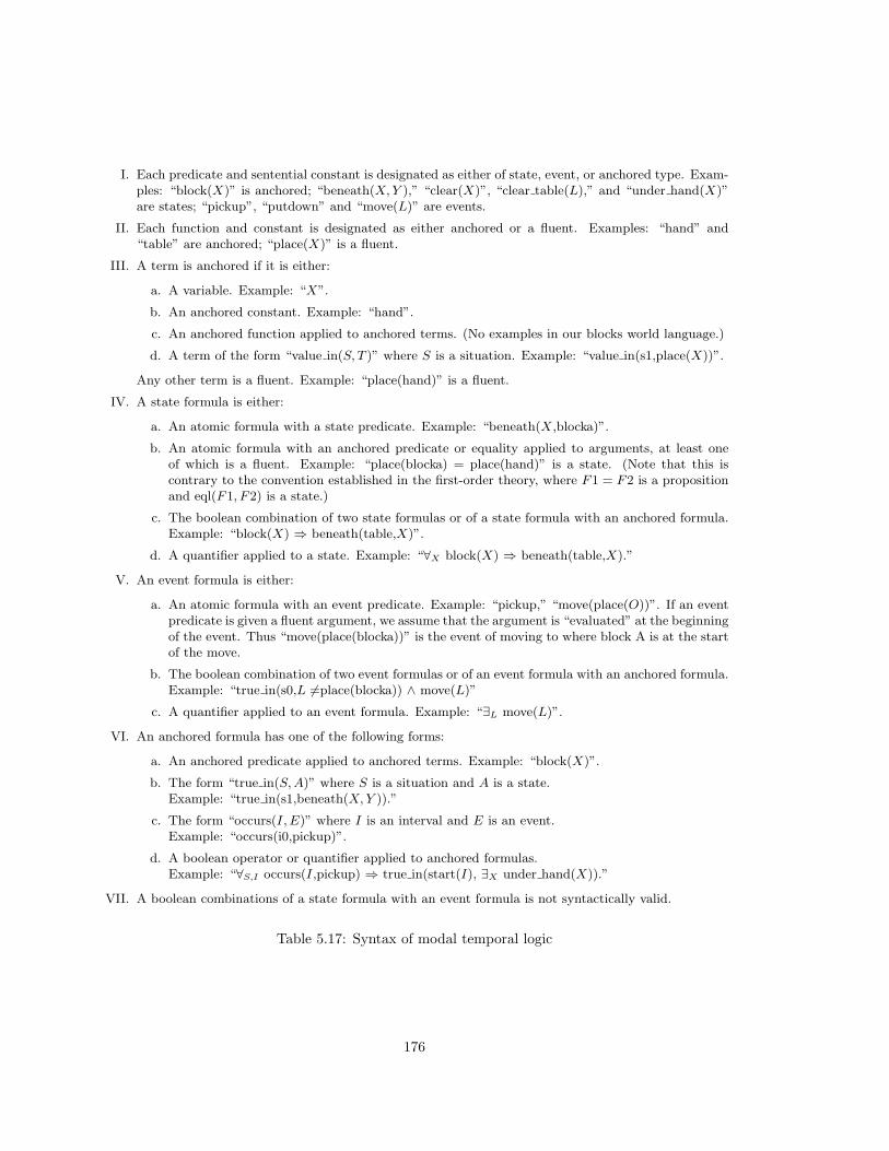
I. Each predicate and sentential constant is designated as either of state, event, or anchored type. Exam-ples: “block(X)” is anchored; “beneath(X, Y ),” “clear(X)”, “clear table(L),” and “under hand(X)”are states; “pickup”, “putdown” and “move(L)” are events.

II. Each function and constant is designated as either anchored or a fluent. Examples: “hand” and“table” are anchored; “place(X)” is a fluent.

III. A term is anchored if it is either:

a. A variable. Example: “X”.

b. An anchored constant. Example: “hand”.

c. An anchored function applied to anchored terms. (No examples in our blocks world language.)

d. A term of the form “value in(S, T )” where S is a situation. Example: “value in(s1,place(X))”.

Any other term is a fluent. Example: “place(hand)” is a fluent.

IV. A state formula is either:

a. An atomic formula with a state predicate. Example: “beneath(X,blocka)”.

b. An atomic formula with an anchored predicate or equality applied to arguments, at least oneof which is a fluent. Example: “place(blocka) = place(hand)” is a state. (Note that this iscontrary to the convention established in the first-order theory, where F1 = F2 is a propositionand eql(F1, F2) is a state.)

c. The boolean combination of two state formulas or of a state formula with an anchored formula.Example: “block(X) ⇒ beneath(table,X)”.

d. A quantifier applied to a state. Example: “∀X block(X) ⇒ beneath(table,X).”

V. An event formula is either:

a. An atomic formula with an event predicate. Example: “pickup,” “move(place(O))”. If an eventpredicate is given a fluent argument, we assume that the argument is “evaluated” at the beginningof the event. Thus “move(place(blocka))” is the event of moving to where block A is at the startof the move.

b. The boolean combination of two event formulas or of an event formula with an anchored formula.Example: “true in(s0,L 6=place(blocka)) ∧ move(L)”

c. A quantifier applied to an event formula. Example: “∃L move(L)”.

VI. An anchored formula has one of the following forms:

a. An anchored predicate applied to anchored terms. Example: “block(X)”.

b. The form “true in(S, A)” where S is a situation and A is a state.Example: “true in(s1,beneath(X, Y )).”

c. The form “occurs(I, E)” where I is an interval and E is an event.Example: “occurs(i0,pickup)”.

d. A boolean operator or quantifier applied to anchored formulas.Example: “∀S,I occurs(I,pickup) ⇒ true in(start(I), ∃X under hand(X)).”

VII. A boolean combinations of a state formula with an event formula is not syntactically valid.

Table 5.17: Syntax of modal temporal logic

176

MTIME.1 Any tautology of the propositional calculus is an axiom.

MTIME.2 If α and β are anchored formulas, then any closure of

[∀µα ∧ ∀µα⇒β] ⇒∀µβ

is an axiom.

MTIME.3 If τ is an anchored term, and α(µ) is a formula with free variable µ then any closure ofα(µ/τ)⇒∃µα(µ) is an axiom.

MTIME.4 For any formulas φ and ψ and boolean operator O, any closure of the formulas below is anaxiom:

true in(S,φ O ψ) ⇔ true in(S, φ) O true in(S, ψ)occurs(I,φ O ψ) ⇔ occurs(I, φ) O occurs(I, ψ)

(Booleans commute with true in and occurs.)

MTIME.5 For any formula φ, variable µ, and quantifier Q, any closure of the formulas below is an axiom:

true in(S,Qµφ) ⇔ Qµtrue in(S, φ).occurs(I,Qµφ) ⇔ Qµoccurs(I, φ)

(Quantifiers commute with true in and occurs.)

MTIME.6 If φ is an anchored proposition then

true in(S, φ) ⇔ φ.occurs(I, φ) ⇔ φ.

(True in and occurs are redundant applied to a anchored proposition.)

MTIME.7 If τ is an anchored term then value in(S, τ) = τ .(Value in is redundant applied to anchored terms.)

MTIME.8 For any predicate symbol β and terms τ1 . . . τk,

true in(S,β(τ1 . . . τk)) ⇔ true in(S,β(value in(S, τ1), . . . value in(S, τk))).

(A predicate holds on fluent arguments just if it holds on the values of the fluents at theanchoring time.)

MTIME.9 For any predicate symbol β and terms τ1 . . . τk,

occurs(I,β(τ1 . . . τk)) ⇔ occurs(I,β(value in(start(I),τ1), . . . value in(start(I),τk))).

(An event term with fluent arguments occurs just if the event term with the values of thearguments at the start of the anchoring interval occurs.)

MTIME.10 For any function symbol β and terms τ1, . . . τk,

value in(S,β(τ1 . . . τk)) = value in(S,β(value in(S, τ1), . . . value in(S, τk))).

(The value in S of a function on fluents is equal to the value in S on their values in S.)

Inference Rules:

Modus Ponens: From α and α⇒β infer β.Necessitation:

If φ is a state proposition then φ ⊢ ∀Strue in(S, φ).If φ is a event proposition then φ ⊢ ∀Ioccurs(I, φ).

Table 5.18: A Modal Temporal Logic

177

true in(S,future(φ)) ⇔ ∀S1>S true in(S1, φ).true in(S,past(φ)) ⇔ ∀S1<S true in(S1, φ).true in(S,some future(φ)) ⇔ ∃S1>S true in(S1, φ).true in(S,some past(φ)) ⇔ ∃S1<S true in(S1, φ).

Table 5.19: Tense operators

BW.3. ¬(beneath(X,Y ) ∧ beneath(Y,X).

BW.4. [ beneath(X,Y ) ∧ beneath(Y,Z)] ⇒ beneath(X,Z)

BW.5. [beneath(table,X) ∧ beneath(table,Y ) ∧ place(X) = place(Y ) ] ⇒[X = Y ∨ beneath(X,Y ) ∨ beneath(Y,X)].

BW.15. after(under hand(X),pickup) ⇒ beneath(hand,X)

BW.16. after(true, move(L)) ⇒ L=place(hand)

BW.17. after(beneath(hand,X) ∧ under hand(Y ), putdown) ⇒ beneath(Y,X).

BW.18. after(beneath(hand,X) ∧ clear table(place(hand)), putdown) ⇒ beneath(table,X)

Table 5.20: Some Modal Blocks World Axioms

was true at some point in the past. Table 5.19 shows how these may be formally defined in

terms of “true in”. (Standard tense logics use only tense operators like these; they do not use the

“true in” operator. The logic provides rules for combining these operators, such as “some past(φ)

⇒ future(some past(φ))”.)

Dynamic modal operators allow events and states to be combined in complex structures. For

example, we could define a modal operator “after(θ, φ)”, which takes as arguments a state θ and an

event φ, and returns the state of just having completed φ after a situation where θ held.

true in(S,after(θ, φ)) ⇔ ∃I end(I)=S ∧ true in(start(I),θ) ∧ occurs(I, φ)

Similarly, the control structures defined in section 5.11 can all be defined as modal operators that

take events and states as arguments and return events. The operator “sequence(φ1, φ2)” maps two

events to an event; “cond(θ, φ1, φ2)” maps a state θ and two events φ1, φ2 to an event; “while(θ, φ)”

maps a state θ and event φ to an event.

Modal language allows many statements to be expressed more compactly and in a form closer

to English. Table 5.20 illustrates the expression of some of the blocks world axioms in terms of the

operators we have defined above.

5.13 Tracking the Present Moment

So far, our representations have viewed all situations as equal sub specie aeternis. Obviously, an

intelligent creature must be able to distinguish the present situation from the past and the future.

The present and immediate past and future almost always deserve considerably more attention than

178

the distant past of future. Perceptions reflect the present and immediate past; actions must be

appropriate to the present and immediate future.

It would seem, however, that the distinguishing of the present cannot be part of the logical

structure of the temporal representation, because which situation is the present continually changes.

Time moves on while reasoning is carried out, or if no reasoning is taking place. The continual

change to the present therefore cannot be the result of an inferential process.

The following architecture can be used for programs that must track the present moment while

doing significant temporal reasoning. The basic knowledge base is a time line, with no indication of

past, present, or future. The program maintains a non-logical pointer to the current situation in the

time-line (or, more realistically, to the latest situation known to be in the past.) The perceptions

received by the system, which can include feedback from the effectors or readings from a clock,

are each tagged as belonging to a particular situation or interval on the time line. As soon as a

perception is incorporated into the time line, the system updates the “now” pointer to indicate that

this perception is in the past. The control mechanisms for the effectors are hard-wired to carry

out the actions planned for the present moment; the control mechanism for the inference engine is

hard-wired to focus its energy on the present moment. ([Subramanian and Woodfill, 1989] studies

an alternative approach in which “now” is used as a formal primitive, and the knowledge base is

continually updated.)

Many programs use a knowledge base that describes only the current situation without temporal

markings. Such an architecture is fine for reasoning for reasoning about the present, but it cannot

be used for any substantial temporal reasoning. A program with a time line may find it useful, for

purposes of efficiency, to maintain a description of the present as an adjunct knowledge base.

5.14 References

Situations were introduced as an AI temporal representation in an early paper on commonsense

reasoning by McCarthy [1963]. Green [1969] used the situation calculus in his QA3 planner.

McCarthy and Hayes [1969] gave a detailed presentation of the situation calculus and a discussion

of the frame problem. Hayes [1978] suggested using histories — chunks of space-time — as an

alternative to situations. McDermott [1982a] modified the situation calculus to deal with continuous,

forward-branching time; the presentation in this chapters is largely based on this work. Allen [1984]

developed a temporal ontology based on the use of intervals, rather than situations. [Shoham, 85b]

is an interesting discussion of the requirements of a temporal theory. [Subramanian and Woodfill,

89] discusses the use of the temporal indexical “now.”

The STRIPS representation was developed in [Fikes and Nilsson, 71]. [Lifschitz, 87c] gives a

logical analysis of this representation.

There is a large body of work on the frame problem, and on solving the frame problem using de-

fault logic, particularly since the Yale Shooting Problem was discovered [Hanks and McDermott, 87].

Particularly significant are [Shoham, 88], [Lifschitz, 87a], [Kautz, 86], [Dean and Kanazawa, 88],

[Morgenstern and Stein, 88] [Morris, 88], [Shoham and McDermott, 88], and [Baker, 89]. [Brown, 87]

is a collection of technical papers on this subject. [Pylyshyn, 87] contains papers by AI researchers,

179

Figure 5.4: Tic-Tac-Toe Board

cognitive scientists, and philosophers discussing the frame problem from a broad perspective.

Implementations of temporal reasoning engines are discussed in [Kahn and Gorry, 77], [Vilain,

82] [Vere, 83], and [Dean, 85].

The reification of event tokens was proposed by Davidson [1967]. Modal logic was first applied

to temporal logic by Prior [1967]; see also [Rescher and Urquhart, 71] and [van Benthem, 83]. Of

related interest is dynamic logic, which has been developed for the formal analysis of computer

programs; see [Pratt, 76], [Harel, 79].

5.15 Exercises

Problems 1-6 can all be carried out using only the simple notation of sections 5.1 — 5.4 of first-

order logic without set theory, without control structures, and without branching time. The student

should be thoroughly familiar with the expressive power of this language before going on to these

more advanced notations.

1. Consider the following microworld: There are lightbulbs, sockets, and switches. Each socket

is controlled by exactly one switch; each switch controls exactly one socket. The following states are

significant: A lightbulb may be in a socket; a lightbulb may be shining or dark; a lightbulb may be

working or burned out; a switch may be on or off. The following events are significant: A switch

may be turned on or off; a lightbulb may be inserted or removed from a socket; a lightbulb may

burn out.

a. Describe the lightbulb domain in a temporal logic.

b. Describe the lightbulb domain in the STRIPS representation.

2. Axiomatize the game of Tic-Tac-Toe. You may assume that a predicate “line(Q1, Q2, Q3)”,

asserting that the three squares Q1, Q2, and Q3 lie in a row, is available. Your axiomatization should

allow the following statements to be expressed: (i) If square Q contains a mark in one situation, it

has the same mark in all later situations. (ii) If the board is as shown in figure 5.4, then, whatever

O plays, X can win on the next turn.

3.* Axiomatize the game of GHOST. You may assume that the following non-logical symbols are

already defined:

180

word(W ) — Predicate: holds if string W is an English word

add letter(W,X) — Function: Maps string W and letter X on to the string that results when

X is added at the end of W .

initial string(W1,W2) — Predicate: Holds if word W1 is an initial string of word W2.

null — Constant. The null string.

next player(P,L) — Function: L is a list of players in order. P is a player. next player(P,L) is

the player who plays after P , according to list L.

drop player(P,L) — Function: L and P are as above. drop player(P,L) is the list L with player

P removed.

single list(P ) — Function: Maps player P onto the list containing only P .

Include the following features: Each player takes turns adding one letter to the end of the string.

A player loses a round, and gains a point, when he completes a word. A player who has five points

has lost the game, and drops out. A player wins when all other players have dropped out.

4. Axiomatize the blocks world with multiple hands, assuming that only one hand can act at a

time.

5.* Axiomatize the blocks world with multiple hands that can act simultaneously.

6. You are trying to get from the train station to the public library. To do this, you must take

the no. 43 bus from the station to downtown, and then take the no. 31 bus from downtown to the

public library. The no. 43 bus comes every 5 minutes, and takes between 12 and 15 minutes to go

from the station to downtown. The no. 31 bus comes every 15 minutes, and takes between 15 and

20 minutes to go from downtown to the library.

a. Formalize this information in an axiomatic system. Show that your axiomatization supports

the inference, “It will take between 27 and 55 minutes to go from the train station to the library.”

b. Add the facts that the 31 bus leaves downtown on the hour, quarter-past, half-past, and

quarter-of, and that you arrive at the train station at two minutes to twelve. Show that your

axiomatization supports the conclusion, “The arrival at the library will either be between 12:30 and

12:35 or between 12:45 and 12:50.”

7. In our representation of branching time, we distinguish only what actually happened as par-

ticularly significant. All other possible situations and chronicles are treated as equally hypothetical.

For this reason, our representation does not allow us to speak of what would have happened under

particular circumstances, as opposed to what could have happened. For example, we would like to

say that Nixon would not have resigned in 1974 if Watergate had not been discovered, though, of

course, he could have in any case. Show how such concept can be represented by defining, for each

situation, real and hypothetical, the “realest” chronicle of that situation; that is, the chronicle that

would occur if that situation came about.

8. In this problem, we will discuss efficient implementation of prediction, using the STRIPS

representation of events. A prediction problem will be specified by giving the relevant states that

hold in the starting situation and the sequence of event types that occur. In the algorithms we are

181

looking for, there will a certain amount of initial processing when the problem is presented. The

system is then equipped to answer quickly queries of the form, “Does state A hold in situation S?”

Assume that no coherence axioms are needed to answer these queries; the relevant states are all

listed in the original situation description or in the add-lists and delete-lists of the events.

Let k be the number of states that hold in the initial situation. Let cA be the number of times

that state A changes its value in the course of the events that occur. Let C be the sum of the sizes

of the add-lists and delete-lists over all the events that occur.

a. Give an algorithm to determine whether state A holds in the final situation S expected

constant O(1) time, using initial processing with expected time O(k + C). (Hint: Since all states

are atomic, one can hash directly on the name of a state type.)

b.* Assuming that the intermediate situations are numerically ordered, give an algorithm to

determine whether state A holds in situation S in expected time O(log(cA)), using initial processing

with expected time O(k + C).

9.* In the modal logic of section 5.12, show that applying existential abstraction and universal

specification to fluents will lead to incorrect results.

182