time-domain reconstruction methods for … university signals and systems time-domain reconstruction...
TRANSCRIPT

Uppsala University
Signals and Systems
Time-domain Reconstruction Methods
for Ultrasonic Array Imaging
A Statistical Approach
Fredrik Lingvall
UPPSALA UNIVERSITY 2004

Dissertation for the degree of Doctor of Philosophyin Electrical Engineering with specialization in Signal Processing, 2004.
ABSTRACTLingvall, F., 2004. Time-domain Reconstruction Methods for Ultrasonic ArrayImaging: A Statistical Approach, 178 pp. Uppsala. ISBN 91-506-1772-9.
This thesis is concerned with reconstruction techniques for ultrasonic array imag-ing based on a statistical approach. The reconstruction problem is posed as theestimation of an image consisting of scattering strengths. To solve the estimationproblem, a time-domain spatially-variant model of the imaging system is devel-oped based on the spatial impulse response method. The image reconstruction isformulated as a linearized inverse-scattering problem in which the time and spacediscrete natures of the imaging setup as well as measurement uncertainties aretaken into account. The uncertainties are modeled in terms of a Gaussian distri-bution. The scattering strengths are estimated using two prior probability densityfunctions (PDF’s), Gaussian and exponential PDF’s. For the Gaussian PDF, themaximum a posteriori (MAP) approach results in an analytical solution in the formof a linear spatio-temporal filter which deconvolves the diffraction distortion dueto the finite-sized transducer. The exponential distribution leads to a positivityconstrained quadratic programming (PCQP) problem that is solved using efficientoptimization algorithms. In contrast to traditional beamforming methods (based ondelay-and-summation), the reconstruction approach proposed here accounts bothfor diffraction effects and for the transducer’s electro-mechanical characteristics.The simulation and experimental results presented show that the performances ofthe linear MAP and nonlinear PCQP estimators are superior to classical beamform-ing in terms of resolution and sidelobe level, and that the proposed methods caneffectively reduce spatial aliasing errors present in the conventional beamformingmethods.
Keywords: Ultrasonic array imaging, synthetic aperture imaging, maximum a pos-teriori estimation, linear minimum mean squared error estimation, SAFT, Bayesianimage reconstruction.
Fredrik Lingvall, Signals and Systems, Uppsala University, P O Box 528,
SE-751 20 Uppsala, Sweden. E-mail: [email protected].
c© Fredrik Lingvall 2004
This thesis has been prepared using LATEX.
ISBN 91-506-1772-9
Printed in Sweden by Eklundshofs Grafiska AB,Uppsala, 2004Distributed by Signals and Systems, Uppsala University, Uppsala, Sweden.

To my parents

iv

Acknowledgments
Many persons have supported and encouraged me in my work as a Ph.D stu-dent. I would especially like to thank my supervisor Prof. Tadeusz Stepinskifor all his help, encouragement, and for giving me the opportunity to workin this very inspiring group. I also want to express my sincere gratitude toDr. Tomas Olofsson for his valuable guidance and support. Much of what ispresented in this thesis is the result of stimulating discussions with TomasOlofsson.
I want to thank Dr. Ping Wu and Prof. Bogdan Piwakowski who havehelped me the most in understanding acoustic wave propagation and acous-tic modeling. It has been very interesting and instructive to develop theacoustic modeling software used in this thesis in cooperation with BogdanPiwakowski.
I am very grateful to Prof. Anders Ahlen for proof-reading (and improv-ing) the manuscript, as well as encouraging me when everything seemedhopeless.
I also acknowledge all the people that work, and have worked, at theSignals and Systems group who have made Magistern such a fun place towork at. In particular, Dr. Mats Gustafsson and Dr. Daniel “kungligt”Asraf for, among other things, our many valuable discussions, and Ove Ew-erlid, for improving my Linux skills. I’m also grateful for the support ofmy “teammates” Mattias Johansson and Nilo Casimiro Ericsson, and to Dr.Sorour Falahati and Prof. Mikeal Sternard for keeping my spirit up whilewriting this thesis!
v

vi
I’m also very grateful to my biking and climbing friends, where our manymountainbike rides, trips to the French Alps and the Norwegian icefalls havehelped me “re-charging my batteries”.
Finally, I would like to express my deepest gratitude to my parents andto my two brothers for your never-ending support. Thank you!
Fredrik Lingvall
Uppsala, September 2004.

CONTENTS
1 Introduction 1
1.1 Basic Ultrasonic Imaging Concepts . . . . . . . . . . . . . . . 3
1.1.1 Ultrasonic Transducers . . . . . . . . . . . . . . . . . . 4
1.1.2 Ultrasonic Image Presentation Methods . . . . . . . . 5
1.1.3 Wave Modes of Elastic Waves . . . . . . . . . . . . . . 10
1.1.4 Ultrasonic Measurement Configurations . . . . . . . . 11
1.2 Conventional Array Imaging . . . . . . . . . . . . . . . . . . . 13
1.3 Problem Formulation . . . . . . . . . . . . . . . . . . . . . . . 21
1.3.1 The Image Formation Model . . . . . . . . . . . . . . 22
1.4 Thesis Contributions and Relation to Earlier Work . . . . . . 24
1.5 Outline of the Thesis . . . . . . . . . . . . . . . . . . . . . . . 27
1.6 Financial Support . . . . . . . . . . . . . . . . . . . . . . . . 29
I Ultrasound Theory and Modeling 31
2 Ultrasound Wave Propagation 33
2.1 The Acoustic Wave Equation . . . . . . . . . . . . . . . . . . 34
2.2 Green’s Functions . . . . . . . . . . . . . . . . . . . . . . . . 35
vii

viii Contents
2.3 Boundary Conditions and Related Integrals . . . . . . . . . . 37
2.3.1 The Rayleigh Integral . . . . . . . . . . . . . . . . . . 37
2.3.2 The Rayleigh-Sommerfeld Integral . . . . . . . . . . . 39
2.3.3 The Kirchhhoff Integral . . . . . . . . . . . . . . . . . 40
2.4 The Convolution Integral . . . . . . . . . . . . . . . . . . . . 41
3 The Spatial Impulse Response 43
3.1 Analytical Solutions for some Canonical Transducer Types . . 44
3.1.1 The Point Source . . . . . . . . . . . . . . . . . . . . . 44
3.1.2 The Line Source . . . . . . . . . . . . . . . . . . . . . 45
3.1.3 The Circular Disc . . . . . . . . . . . . . . . . . . . . 46
3.2 Sampling Analytical Spatial Impulse Responses . . . . . . . . 48
3.3 The Pressure Field . . . . . . . . . . . . . . . . . . . . . . . . 50
3.4 A Numerical Method for Computing Spatial Impulse Responses 51
3.A The Rectangular Source . . . . . . . . . . . . . . . . . . . . . 56
3.B An Algorithm for Computing SIRs in Immersed Solids . . . . 59
4 A Discrete Linear Model for Ultrasonic Imaging 63
4.1 Model Assumptions . . . . . . . . . . . . . . . . . . . . . . . 64
4.2 A Linear Imaging Model . . . . . . . . . . . . . . . . . . . . . 65
4.3 A Discrete Two-dimensional Model . . . . . . . . . . . . . . . 68
II Methods based on Delay-and-sum Focusing 73
5 The Synthetic Aperture Focusing Technique 75
5.1 The SAFT Algorithm . . . . . . . . . . . . . . . . . . . . . . 77
5.2 Performance of The Synthetic Aperture Focusing Technique . 79
5.2.1 Spatial Undersampled Broadband Data . . . . . . . . 80
5.2.2 Finite Sized Transducers and Lateral Resolution . . . 84
5.3 Matrix Formulation of the SAFT Algorithm . . . . . . . . . . 85
5.4 Matched Filter Interpretation . . . . . . . . . . . . . . . . . . 88
5.5 Remarks . . . . . . . . . . . . . . . . . . . . . . . . . . . . . . 88

Contents ix
6 Real Aperture Array Imaging 91
6.1 Conventional Narrowband Transmit Beamforming Analysis . 92
6.2 Broadband Transmit Beamforming with Finite Sized ArrayElements . . . . . . . . . . . . . . . . . . . . . . . . . . . . . 93
6.3 Parallel Receive Beamforming . . . . . . . . . . . . . . . . . . 98
III Bayesian Ultrasonic Image Reconstruction 101
7 Ultrasonic Image Reconstruction Methods 103
7.1 Bayesian Image Reconstruction . . . . . . . . . . . . . . . . . 106
7.1.1 Assigning Prior Probability Density Functions — TheMaximum Entropy Principle . . . . . . . . . . . . . . 109
7.1.2 The Optimal Linear Estimator . . . . . . . . . . . . . 114
7.1.3 The Optimal Beamformer with Exponential Prior . . 116
7.2 Focusing as an Inverse Problem . . . . . . . . . . . . . . . . . 116
7.2.1 Singular Value Decomposition Inversion . . . . . . . . 118
7.2.2 Tikhonov Regularization . . . . . . . . . . . . . . . . . 118
7.2.3 The Maximum Likelihood Estimator . . . . . . . . . . 120
7.3 Concluding Remarks . . . . . . . . . . . . . . . . . . . . . . . 121
7.A Some Matrix Derivations . . . . . . . . . . . . . . . . . . . . . 122
7.A.1 Equivalence of MAP and Linear MMSE Estimators . 122
7.A.2 Performance of the Linear MMSE and MAP Estimators122
8 Applications 125
8.1 Experimental Equipment . . . . . . . . . . . . . . . . . . . . 126
8.2 Ultrasonic Synthetic Aperture Imaging . . . . . . . . . . . . . 127
8.2.1 The Monostatic Propagation Matrix . . . . . . . . . . 127
8.2.2 Lateral Resolution and Finite Sized Transducers . . . 130
8.3 Parallel Array Imaging . . . . . . . . . . . . . . . . . . . . . . 137
8.3.1 The Propagation Matrix for Parallel Receive Imaging 137
8.3.2 The Optimal Linear Estimator . . . . . . . . . . . . . 139
x Contents
8.3.3 Grating Lobe Suppression of the Optimal Linear Es-timator . . . . . . . . . . . . . . . . . . . . . . . . . . 139
8.4 Parallel Imaging with Exponential Priors . . . . . . . . . . . 145
8.4.1 Remarks . . . . . . . . . . . . . . . . . . . . . . . . . . 156
8.5 Summary . . . . . . . . . . . . . . . . . . . . . . . . . . . . . 156
9 Performance of the Optimal Linear Estimator 159
9.1 The Normalized Expected Error . . . . . . . . . . . . . . . . 160
9.2 Parallel Array Imaging Performance . . . . . . . . . . . . . . 161
10 Concluding Remarks and Future Research 167
Bibliography 170

Contents xi
Glossary
Notational conventions
Matrices and vectors are denoted using boldface Roman letters and scalarsare denoted using lowercase Roman or Greek letters throughout the thesis.All matrices are expressed using boldface upper-case letters and all vectorsare, by convention, column vectors.
Two types of vectors occur in the thesis. One type denote the positionalvectors that are used when presenting the sound model. These three dimen-sional vectors are expressed using r and sometimes have a sub and/or superscript. For instance, rt denotes the position of a point-like target.
The vectors of the second type are of higher dimension. These vectorstypically consist of vectorized matrices or of samples from a signal or noisesequence. A vectorized matrix a is defined by
a , vec(A) = [aT0 aT
1 · · ·aTJ ],
where aj denotes the jth column in A and J is the total number of columnsin A.
Symbols
Below the most frequently used symbols in the thesis are summarized:∗ Convolution in time.= Rounding towards the nearest integer
, Equality by definitionAT The transpose of matrix A
aj The jth column of matrix A
(A)m,n Element (m, n) in matrix A
vec(·) Operator that transforms a matrix lexicographically to a vectorE The expectation operator with respect to signals||x||2 The L2 norm of the vector x (||x||2 = xTx)tr{·} The trace of a matrix (tr{A} =
∑
i(A)i,i)|A| The determinant of the matrix A
t Timek Discrete-time indexf Frequency in Hertz

xii Contents
ω Angular frequency (ω = 2πf)Fs Sampling frequencyTs Sampling period (Ts = 1/Fs)Ce Covariance matrix of e
Co Covariance matrix of o
I The identity matrix
0 The null matrix of suitable dimensionδ(t) Delta function (in continuous-time)wn Apodization weightvn(t) Normal velocitySb
RSurface of a transducer in receiving (backward) mode
SfR
Surface of a transducer in transmit (forward) modecp Longitudinal (primary) sound speedρ0 Medium densityr A general field pointrt A field point of a point-like targetrrr A point on the receive (backward) transducer’s surface
rfr A point on the transmit (forward) transducer’s surface
Abbreviations
ADC Analog-to-Digital ConverterDREAM Discrete REpresentation Array ModelingDAS Delay-and-SumCW Continuous WaveFIR Finite Impulse ResponseHPBW Half-power BandwidthIID Independent and Identically DistributedIIR Infinite Impulse ResponseLS Least SquaresLTI Linear Time-InvariantMAP Maximum A Posteriori
MF Matched FilterMMSE Minimum Mean Squared ErrorML Maximum LikelihoodMSE Mean Squared ErrorMCMC Markov Chain Monte-CarloNDE Nondestructive Evaluation

Contents xiii
NDT Nondestructive TestingPA Phased ArrayPDE Partial Differential EquationPDF Probability Density FunctionPSF Point Spread FunctionQP Quadratic ProgrammingRF Radio FrequencyROI Region-of-InterestSAI Synthetic Aperture ImagingSAFT Synthetic Aperture Focusing TechniqueSDH Side-drilled HoleSNR Signal-to-Noise RatioSAR Synthetic Aperture RadarSAS Synthetic Aperture SonarTOFD Time-of-Flight Diffraction

xiv Contents

CHAPTER 1
Introduction
ACOUSTIC array imaging is a technique used in many fields such asmedical diagnostics, sonar, seismic exploration, and non-destructive
testing. The objective with acoustic imaging, in general, is to localize andcharacterize objects by means of the acoustic scattered field that they gen-erate. An array of sensors facilitates this task since the diversity introducedby transmitting and receiving acoustic energy from many positions enableslocalization of the scatterers.1 In other words, by using an array it is possibleto both localize remote objects and estimate their scattering strengths.
In contrast to electromagnetic array imaging, where narrow band signalswith wavelengths exceeding the array antenna elements are used, broadbandpulsed waveforms are commonly used in acoustic array imaging. The wave-length corresponding to the center frequency of these pulses is often of thesame size as the array elements. This make diffraction effects apparentresulting in a frequency dependent beam directivity of the array elements.
Array imaging is, in this thesis, understood as a process which aimsat extracting information about the scattering strength of an object understudy. A realistic model of the imaging system is required to perform asuccessful imaging.
The aim of this thesis is to develop and explore new model based imaging
1Acoustic arrays have also become popular since they are less expensive than, forexample, X-ray computerized tomography (CT) or magnetic resonance imaging (MRI)systems [1].
1

2 Chapter 1. Introduction
methods by utilizing the spatial diversity inherent in array systems by takingdiffraction effects as well as the broadband pulsed waveforms into account.This is performed using a model-based approach where the model is obtainedfrom the known geometry and electro-mechanical characteristics of the array.
A suitable model can be obtained by solving the forward problem ofwave propagation. The main objective in acoustic array imaging is, however,finding a solution to the backward, or the inverse problem, which is definedhere as image reconstruction from the ultrasound data. More specifically, theimage under consideration, which consists of the scattering strength at everyobservation point in the region-of-interest (ROI), has to be estimated fromthe received acoustic field. That is, the image cannot be measured directly,it can only be observed indirectly through the scattered field measured atthe (limited) array aperture which, furthermore, is distorted due to theelectro-mechanical characteristics of the measurement system. Therefore,the image has to be estimated, or reconstructed, from the observed data.This can be seen as a process of removing the effects of the observationmechanism, which in our case is the processing needed to compensate forthe wave propagation effects and the electro-mechanical properties of thearray.
Traditionally, acoustic array data has been processed by means of spatialfiltering, or beamforming, to obtain an image of the scattering objects [2–4]. Beamforming using the classical time-domain delay-and-sum method isanalogous to the operation of an acoustical lens and it can be performedefficiently using delay-line operations in real time or using post-processingas in synthetic aperture systems [5–8]. Conventional beamforming, whichis essentially based on a geometrical optics approach [9], is computationallyattractive due to its simplicity but is has several inherent drawbacks. Inparticular, conventional beamforming does not perform well in situationswhere the ultrasound data is obtained using an array that is sparsely sampledwhich, unfortunately, is quite common in many applications.
The main motivation for developing the reconstruction algorithms dis-cussed in this thesis is the need to improve the performance of traditionalultrasonic array imaging methods. To overcome, or at least alleviate, theproblems with conventional beamformers, a model based time-domain ap-proach is proposed here. It takes into account the diffraction pattern of anarbitrary array setup. This model accounts for all linear effects, such as,transducer size effects, side- and grating lobes, focusing, and beam steering.By a proper design of the reconstruction algorithm it should be possibleto compensate such effects and thereby achieve reconstruction performance

1.1. Basic Ultrasonic Imaging Concepts 3
superior to conventional array imaging.
The rest of the chapter is organized as follows: In Section 1.1, some basicconcepts in ultrasonic array imaging are presented. In particular an intro-duction to elastic wave propagation, scattering and array image formationis given. This is followed by Section 1.2, where conventional array imaging,or beamforming is discussed. Section 1.3 presents the general formulation ofthe array imaging problem, and in Section 1.4 the contributions of this the-sis are summarized. A short review of earlier related work is also presented.Finally, Section 1.5 gives the outline of this thesis.
1.1 Basic Ultrasonic Imaging Concepts
The basic physical property behind ultrasonic imaging is that an impingingacoustical wave is scattered by a discontinuity, that is, a change in the acous-tic impedance of an otherwise homogeneous object. The received scatteredwave is then converted to an electric signal which normally is sampled andstored in a computer, or a dedicated ultrasonic instrument.
The scattering is governed by a change in the density, ρ, and soundspeed, c, of the inspected specimen. The reflected and transmitted pressureamplitudes are described by the transmission and reflection coefficients, Tt
and Tr respectively. For a planar discontinuity, these coefficients are givenby the acoustic impedance, z1 = ρ1c1, before the discontinuity, and theacoustic impedance, z2 = ρ2c2, after the discontinuity, where ρ1 and ρ2 arethe respective densities and c1 and c2 the corresponding sound speeds. Letpi denote the incident pressure. Then the pressure of the reflected wave, pr,is given by [10]
pr = Trpi =z2 − z1
z2 + z1pi (1.1)
and the pressure of the transmitted wave, pt, is
pt = Ttpi =2z2
z2 + z1pi. (1.2)
For a hard discontinuity we have that z2 > z1 and and for a soft z2 < z1. Forsoft scatterers, the reflection coefficient is negative, which physically resultsin a phase shift at the boundary of the scatterer.2
2Later when the reconstruction algorithms are discussed it will be shown that thereconstruction performance can be improved if it is known a priori whether the scattereris hard or soft.

4 Chapter 1. Introduction
The acoustic waves are generated using a transducer which convertsan electrical waveform to an acoustical (or elastic) wave and vice versa.3
The driving input signal to the transducer is normally a sinusoidal signal,resulting in a narrowband continuous wave (CW), or a pulsed broadbandsignal.
In CW imaging it is difficult to separate the scattered and the incidentfield. This is normally solved by using tone-burst signals that still are nar-rowband but allow for a sufficient time separation between the transmittedand received signals.4 Henceforth in this thesis it will be assumed that therealways is a sufficient time separation between the transmitted and receivedwaveforms.
1.1.1 Ultrasonic Transducers
Good acoustic coupling between the transducer and the specimen/mediumis required for an acoustic wave to propagate efficiently into the specimen.Therefore many types of transducers are available to suit different appli-cations. The two perhaps most common types are contact and immersiontransducers. Contact transducers are common in non destructive evalua-tion (NDE) applications where the transducer is placed on the surface ofthe specimen, normally with a couplant gel or water between the trans-ducer and the specimen’s surface to provide sufficient wave transfer into thespecimen.
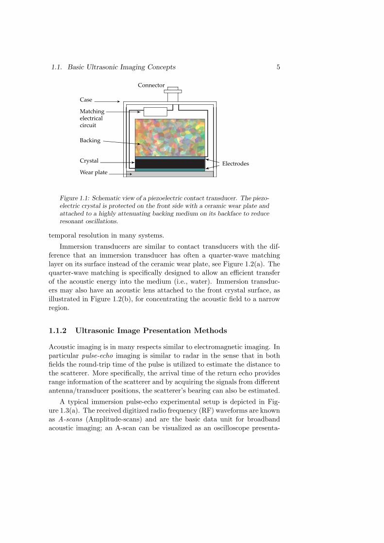
The most common type of transducer is the piezoelectric transducerwhich is used for both contact and immersion measurements. A typicalpiezoelectric contact transducer is shown in Figure 1.1. The piezoelectriccrystal is plated on both sides to create electrodes where the driving inputsignal can be applied. If an electrical signal is applied to the electrodes, thenthe crystal will expand and thereby generate an acoustic wave. The crystal ofa contact transducer is also normally protected with a ceramic wear plate.Moreover, the backface of the crystal is loaded with a highly attenuatingmedium, the so-called backing, which controls the shape and duration ofthe output waveform. Without the backing the transducer would have avery distinct resonant frequency resulting in a narrowband system, that is,the transducer would have a long impulse response which deteriorates the
3If one makes the comparison with sound waves then the transducer acts both as amicrophone and a as loudspeaker.
4In some applications, for example sonar, frequency sweeped chirp signals are alsocommon.
1.1. Basic Ultrasonic Imaging Concepts 5
Matchingelectrical circuit
Backing
ElectrodesCrystal
Connector
Wear plate
Case
Figure 1.1: Schematic view of a piezoelectric contact transducer. The piezo-electric crystal is protected on the front side with a ceramic wear plate andattached to a highly attenuating backing medium on its backface to reduceresonant oscillations.
temporal resolution in many systems.
Immersion transducers are similar to contact transducers with the dif-ference that an immersion transducer has often a quarter-wave matchinglayer on its surface instead of the ceramic wear plate, see Figure 1.2(a). Thequarter-wave matching is specifically designed to allow an efficient transferof the acoustic energy into the medium (i.e., water). Immersion transduc-ers may also have an acoustic lens attached to the front crystal surface, asillustrated in Figure 1.2(b), for concentrating the acoustic field to a narrowregion.
1.1.2 Ultrasonic Image Presentation Methods
Acoustic imaging is in many respects similar to electromagnetic imaging. Inparticular pulse-echo imaging is similar to radar in the sense that in bothfields the round-trip time of the pulse is utilized to estimate the distance tothe scatterer. More specifically, the arrival time of the return echo providesrange information of the scatterer and by acquiring the signals from differentantenna/transducer positions, the scatterer’s bearing can also be estimated.
A typical immersion pulse-echo experimental setup is depicted in Fig-ure 1.3(a). The received digitized radio frequency (RF) waveforms are knownas A-scans (Amplitude-scans) and are the basic data unit for broadbandacoustic imaging; an A-scan can be visualized as an oscilloscope presenta-

6 Chapter 1. Introduction
Quarter-wave plate
(a) A piezoelectric immersiontransducer. The quarter-waveplate is designed to allow an ef-ficient energy transfer into thewater.
Acoustic lens
(b) A piezoelectric focusedimmersion transducer. Theacoustic lens concentrates theacoustic energy to a narrow re-gion.
Figure 1.2: Illustration of immersion transducers.
tion of the received waveform as shown in shown in Figure 1.3(b).
As mentioned above, the round-trip time of the echo yields informationabout the range to the scatterer. This information is, however, ambigu-ous since many scatterer positions can result in identical round-trip times.Therefore, to enable localizing scatterers, it is necessary to sample the wavefield spatially by moving the transducer or by using several transducers. Animage obtained by a linear movement of the transducer and coding the re-ceived waveform amplitudes, from many transducer positions, in colors oras gray levels is usually denoted a B-scan. An example B-scan is shown inFigure 1.3(c) and if the scatterer is located along the scanning direction,the distance, zsc, between the transducer and the scatterer can be computedfrom the shortest roundtrip-time, trt, found in the B-scan, that is, trt = 2zsc
c .
If the scatterers are located in a certain volume then a surface scancan be performed resulting in a 3D data volume. A common technique tovisualize 3D data in acoustical imaging is the so-called C-scan. A C-scancan be thought of as a photograph taken from above the specimen, obtainedby taking the maximum value of the received A-scans in a particular time-frame. Figure 1.3(d) shows an example C-scan and it can now be seen thatthe scattering energy is concentrated, or “has a peak”, at x = y = 0.
The resolution in B- and C-scan imaging is determined primarily bythe beam shape of the used transducer. Using a highly diffracting (small)transducer results in poor lateral resolution and using a large or focused

1.1. Basic Ultrasonic Imaging Concepts 7
Transducer
Scatterer
Acoustic Wavex
y
z
(a) A typical immersion pulse-echomeasurement setup.
60 65 70 75 80
−1
−0.5
0
0.5
1
t [µs]
Nor
mal
ized
Am
plitu
de
(b) A-scan (Amplitude-scan) plot.
x [mm]
t [µs
]
−5 −4 −3 −2 −1 0 1 2 3 4 5
60
65
70
75
80
(c) B-scan image obtained by a hor-izontal movement of the transducer.The amplitudes of the waveforms cor-responding to each transducer positionis coded as gray levels in the B-scan.
x [mm]
y [m
m]
−5 −4 −3 −2 −1 0 1 2 3 4 5
−5
−4
−3
−2
−1
0
1
2
3
4
5
(d) C-scan image obtained byscanning the transducer in thexy-plane. A C-scan is formedby taking the maximum valueof the received A-scans in aparticular time-frame.
Figure 1.3: Common data presentations types in pulse-echo ultrasonic imag-ing.
8 Chapter 1. Introduction
transducer improves the resolution. This is analogous with optical imagingwhere the sharpness of the image is improved by using a lens. In acousticalimaging, the acoustic lens compensates for the arrival times of the soundwaves originating from the focal zone of the lens, yielding a coherent sum-mation of those waves. The width and depth of the focal zone depends ofthe aperture and focusing depth of the lens. A larger lens has a more nar-row focal zone than a small lens focused at the same depth [9]. Acousticimaging using physical lenses may therefore require repeated scanning withdifferent large aperture lenses, focused at different depths, to obtain volumedata with sufficient resolution.
A-, B- and C-scan imaging are the most rudimentary methods used inacoustical imaging where almost no processing of the data is required. Theyenable, by simple means, visualization of the scattering strengths but theirusefulness is also, somewhat limited. In particular, the user that observesthe images must be skilled enough to be able to interpret the results, whichcan become rather complicated since responses from many scatterers maybe superimposed. The mechanical scanning required to form an image whenusing physical lenses is also time consuming which limits the image framerate. For these and other reasons, imaging using physical lenses is oftenimpractical or even unfeasible. Therefore, a considerable interest has beenobserved in lensless acoustic imaging and array imaging where focusing canbe performed after acquiring data, as in synthetic aperture imaging or inreal time by using physical array systems. It will be shown later in thisthesis that the use of computer analysis can yield further improvementssince signal processing can contribute to a substantial improvement of theresulting images.
Image Display Methods for Broadband Sound Fields and Sig-
nals
Properties, such as, lateral- and temporal resolution, contrast etc are impor-tant measures in ultrasonic imaging. For CW signals and far-field analysisthere exist well established presentation methods, as we will describe in Sec-tion 1.2 below, but for broadband and near-field data special presentationmethods are required. To facilitate evaluation of broadband data, four differ-ent display methods are used in this thesis, each one of which being suitablefor a different purpose. The display methods are shown in Figure 1.4 usingexample waveform data from a 1D array simulation. Figure 1.4(a) shows3D snapshot graph of a (simulated) broadband waveform at one time in-

1.1. Basic Ultrasonic Imaging Concepts 9
(a) 3D snapshot.
−20 −10 0 10 200
0.1
0.2
0.3
0.4
0.5
0.6
0.7
0.8
0.9
1
x [mm]
Nor
mal
ized
Am
plitu
de
(b) Profile plot.
x [mm]
z [m
m]
−50 −40 −30 −20 −10 0 10 20 30 40 50
60
65
70
75
80
85
90
(c) 2D snapshot.
30 35 40 45 50 55
−1
−0.8
−0.6
−0.4
−0.2
0
0.2
0.4
0.6
0.8
1
z [mm]
Nor
mal
ized
Am
plitu
de
(d) On-axis waveform.
Figure 1.4: Image display methods used in throughout the thesis.
stant. Also shown in the 3D graph is the profile of the acoustic field, thatis, a projection of the maximum amplitudes of the field on the x-axis. Thisprofile plot is also shown in Figure 1.4 (b). In Figure 1.4(c) a 2D image ofthe waveform is depicted, whereas in Figure 1.4(d) the on-axis waveform isdisplayed. These four display methods will be used to present both pressurewaveforms, of the type shown in Figure 1.4, and reconstructions, that is, animage or estimate of the insonified object’s scattering strength obtained byprocessing ultrasound data.
10 Chapter 1. Introduction
The profile plot can be seen as the broadband counterpart to the CWbeampattern plot which is suitable for studying the lateral resolution or thecontrast. The temporal or on-axis resolution is most easily studied usingplots of the type shown in Figure 1.4(d). The 2D and 3D plots are suitableto obtain an overall view of a wavefield or a reconstruction.
1.1.3 Wave Modes of Elastic Waves
In addition to the comparison with radar imaging above, it should be notedthat, even though radar and acoustic pulse-echo imaging have many sim-ilarities there are also some fundamental differences. The most apparentdifference is that elastic waves, as opposed to electromagnetic waves havemany propagation modes.
The two dominating modes in acoustic imaging are longitudinal or pres-
sure waves and shear or transversal waves [10, 11]. In longitudinal wavepropagation, the particle displacement is in the same direction as the prop-agation whilst the particle displacement is orthogonal to the propagationdirection for shear waves. In liquids and gases, shear wave propagation isstrongly attenuated and only the longitudinal mode will therefore propa-gate. In solids, both longitudinal and shear waves can propagate. The wavemodes have different sound speeds and the longitudinal sound speed, cp, inmetals is roughly twice the shear wave speed.
Furthermore, elastic wave propagation is complicated by the fact thatmode conversion occurs at a non-normal reflection and refraction at a dis-continuity inside a test specimen, e.g., a metal test object. A typical ex-ample, from NDE imaging, is the multiple mode conversions that can occurat cracks [12]. There, mode conversion generates both longitudinal andshear diffracted waves at the tips of the crack. A surface wave may alsobe generated along the crack, which has different sound speed compared tolongitudinal and shear waves, resulting in additional diffracted waves at thecrack ends [13]. The resulting received signals may therefore consist of amix of different wave modes which may be very difficult to discriminate.Fortunately, in many applications the echoes, corresponding to each wavemode can be resolved since they will arrive with a time separation causedby the different sound speeds of the wave modes.
In the work presented in this thesis all measurements have been per-formed in water in order to avoid mode converted waves and thereby simpli-fying the interpretation of the obtained results. The only exception wherelongitudinal-shear-longitudinal mode conversion could possibly occur was

1.1. Basic Ultrasonic Imaging Concepts 11
in an experiment with scatterers inside an immersed copper block. Thatexperiment was, however, performed in such way that only the non-modeconverted longitudinal waves could arrive in the given time frame.
1.1.4 Ultrasonic Measurement Configurations
So far, we have mostly discussed acoustic imaging using a single, possiblescanned, transducer. Such imaging systems are cost effective but the acqui-sition frame rate is insufficient for many applications. Also, the resolution inB-scan images, obtained from mechanically scanned systems, is defined bythe beampattern of the transducer. As noted above, high resolution B-scanimaging therefore normally requires focused transducers and, consequently,the focusing depth cannot be changed during acquisition in a flexible man-ner. On the other hand, array imaging does not have these limitationsand therefore, a considerable interest in array imaging methods has beenobserved.
Array imaging methods can be classified in two groups: synthetic aper-
ture imaging and physical array imaging. In synthetic aperture imaging thearray aperture is obtained by processing sequentially recorded data from dif-ferent transducer positions, typically using a small transducer with a widebeampattern. Thus, transmit focusing cannot be achieved in synthetic ar-ray imaging and focusing can only be performed in the receive mode onthe recorded data. On the other hand, a physical array comprising severaltransducer elements allows for both steering and focusing of the transmittedbeam. A physical array can also be rapidly re-focused enabling fast beamsweeping systems. Physical array systems have therefore become popular, inparticular, in medical imaging where real-time imaging is of great interest.
Historically, a distinction has been made between linear and phased
(physical) arrays. A linear array system does not have any delay-line cir-cuitry that enables focusing of the transmit beam. Instead, linear arraysare used for fast electronic scanning by switching among the active elementsof the array. Phased array systems, on the other hand, are able to bothsteer and focus the beam by applying suitable time delays on the drivinginput signals to the array elements. The array that has been used in theexperiments presented in this thesis is of the latter type and is consequentlycapable of focusing the beam.
An array system, whether synthetic or physical, can be classified accord-ing to its configuration as shown in Figure 1.5. Monostatic configurations,shown in Figure 1.5(a), are common in synthetic aperture imaging where the

12 Chapter 1. Introduction
Target Region
Transmitter and receiver
(a) Monostatic.
Target Region
Transmitter Receiver
(b) Bistatic.
Target Region
Transmi�ers Receivers
(c) Multistatic.
Target Region
Transmitting Array
Receiving Array
(d) Transmission.
Figure 1.5: Common array measurement methods.
same transducer is used both in transmit and receive mode. Bistatic systems,also known as pitch-catch systems, are used in, for example, NDE applica-tions to detect diffraction echos from crack tips, i.e., time-of-flight diffraction
(TOFD) imaging [14]. A bistatic system is shown in Figure 1.5(b). Physicalarrays can be classified as multistatic, see Figure 1.5(c), since many ele-ments are used simultaneously both in transmit and receive mode. Finally,in transmission imaging, shown in Figure 1.5(d), the specimen is locatedbetween two transducers or physical arrays.
The above presented nomenclature will be used throughout this thesis.Note however that we will primarily consider monostatic and multistatic

1.2. Conventional Array Imaging 13
configurations.
1.2 Conventional Array Imaging
In order to obtain a high resolution image from array data, the data must becompensated for the effect of the wave propagation and the array imagingsystem. The classical method to solve this problem is array beamforming.In this section we will present the basic properties of classical beamforming.This is done in order to introduce the reader not familiar with array imagingto the subject, but also to introduce concepts used later in the thesis.
As mentioned above, the operation principle of a beamformer in conven-tional array imaging is the same as that of an acoustic lens. The basic ideais to impose delays on the transmitted and/or received signals so that thetransmitted acoustic energy or the received signals are combined coherentlyat a focusing point while other signals are combined incoherently. A beam-former can be implemented using both analog delay-line circuits or usingdigital hardware [15, 16].
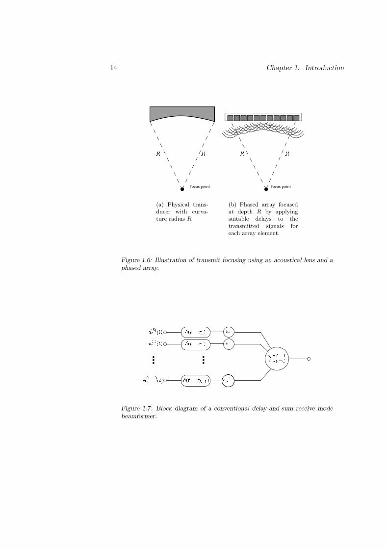
The transmit focusing operation of an acoustical lens and a phased arrayis illustrated in Figure 1.6. Focusing of the acoustical lens, shown in Fig-ure 1.6(a), is achieved by the curvature of the aperture whereas the phasedarray is focused at the same point by imposing time-delays that correspondsto the curvature of the lens.
Reception of the beamformer is analogous to the transmission processand the delays of the received signals can be implemented using delay-linecircuitry and a summing amplifier or by digital shift operations. The opera-tion of a receive mode beamformer is illustrated by the block-diagram shownin Figure 1.7. The time-delays, for the corresponding array elements, aredenoted τn for n = 0, 1, . . . , L− 1, where L is the number of array elements.
The output signal for the nth element is denoted u(n)o (t) and wn is an aper-
ture tapering (or apodization) weight. Apodization, which will be discussedin more detail below, is a somewhat crude method, originating from spectralanalysis, used to control the sidelobe levels in linear beamforming.
The simple delay-and-sum (DAS) operation of the beamformer does nottake any directivity of the array elements into account, hence the elementsare treated as point sources/receivers. Assuming that the point source ele-ment model is viable for the array, the performance of the DAS beamformercan be analyzed in the frequency domain by considering a sum of phase-shifted spherical waves. The response for a sinusoidal source, at the point
14 Chapter 1. Introduction
Focus point
(a) Physical trans-ducer with curva-ture radius R
Focus point
(b) Phased array focusedat depth R by applyingsuitable delays to thetransmitted signals foreach array element.
Figure 1.6: Illustration of transmit focusing using an acoustical lens and aphased array.
Figure 1.7: Block diagram of a conventional delay-and-sum receive modebeamformer.

1.2. Conventional Array Imaging 15
(x, z), can then be expressed as [9]
H(x, z) =L−1∑
n=0
ejω(t−Rn/cp)
Rnwnejωτn , (1.3)
where cp is the sound speed, wn an apodization weight, andRn =
√
(xn − x)2 + z2 is the distance from the observation point to the ntharray element positioned at (xn, 0), see Figure 1.8. The phase-shift due to
(x,z)
xn-x
xn
Rn
d
DArray aperture
Pitch
Figure 1.8: A 1D array with an array pitch d and an aperture D.
the propagation distance from the observation point to the nth element isgiven by ωRn/cp and the phase-shift ωτn is due to the focusing operation.
Conventional Beampattern Analysis
In this thesis we are primarily concerned with broadband array imaging andmodeling, since broadband modeling offers an accurate description of theimaging system. However, array imaging performance is often analyzed us-ing narrowband and far-field approximations. We will discuss the differencesbetween narrowband and broadband analysis in later chapters of this thesis,and a short introduction to narrowband analysis is, therefore, given here.
To simplify the analysis the paraxial approximation is normally appliedwhich means keeping only up to second order terms in the Taylor expansionof Rn in the phase term in (1.3) and only the zero-order term for the ampli-tude term, 1
Rn, and also assuming that (xn − x)2 � z2. In such case a Rn
reduces to Rn ≈ z + (x−xn)2
2z in the phase term.

16 Chapter 1. Introduction
Consider now focusing at the point (0, z). Using the paraxial approxi-mation, the focusing delays are given by
τn∼= 1
cp(z +
x2n
2z), (1.4)
and the response of a source at (x, z), after focusing will be
H(x, z) ∝ ejω(t− x2
2zcp)
L−1∑
n=0
ejωxxn
zcp . (1.5)
After performing the summation in (1.5) the following expression definingthe magnitude of H(x, z), or the beampattern is obtained
|H(x, z)| ∝∣∣∣∣∣
sin(Lπxdλz )
sin(πxdλz )
∣∣∣∣∣, (1.6)
where λ is the acoustic wavelength. The beampattern can also be expressedas a function of the angle, θ, from the center axis of the array to the sourcepoint, (x, z), which in the far-field is given by
|H(θ)| ∝∣∣∣∣∣
sin(Lπ sin(θ)dλ )
sin(π sin(θ)dλ )
∣∣∣∣∣. (1.7)
To illustrate the behavior of the DAS beamformer, two normalized beam-patterns, computed using (1.7) for a phased array focused at (0, z), areshown in Figure 1.9. The beampatterns obtained for the same apertureD = 8λ are plotted as a function of the angle θ for two different arraypitches, d = λ/2 and d = 2λ. Noticeable is that the array pitch does not in-fluence the main beam width or the amplitude of the sidelobes. The width ofthe main beam or the lateral resolution can only be improved by increasingthe aperture, D. To see this, consider the standard criterion for resolvingtwo point sources known as the Rayleigh criterion [9]. The Rayleigh crite-rion is based on the idea that two point sources of equal amplitude can beseparated if the first source is placed at the maximum point of the beam-pattern, x = 0, and the second source at a point where the beampattern iszero. The first zero of the beampattern occur at the distance
dx =λz
Ld=
λz
D= λF, (1.8)
where F = z/D is the so-called F -number. The Rayleigh criterion, whichis a rough measure of the lateral resolution attainable by a physical lens or

1.2. Conventional Array Imaging 17
−60 −50 −40 −30 −20 −10 0 10 20 30 40 50 60−40
−35
−30
−25
−20
−15
−10
−5
0
5
θ [deg]
Nor
mal
ized
Am
plitu
de [d
B]
(a) d = λ/2.
−60 −50 −40 −30 −20 −10 0 10 20 30 40 50 60−40
−35
−30
−25
−20
−15
−10
−5
0
5
θ [deg]
Nor
mal
ized
Am
plitu
de [d
B]
(b) d = 2λ.
Figure 1.9: Beampatterns for a phased array focused at x = 0, with anaperture of 8λ, and wn ≡ 1. The beampattern in (a) is for an array with apitch d = λ/2 and in (b) for an undersampled array with a pitch d > λ/2.
a classical array imaging, states that the resolution is determined by theproduct of the wavelength and the F -number.
Another characteristic feature of classical array imaging can be seen inFigure 1.9(b). Here, the array pitch d is 2λ, and aliased lobes are apparentat θ = 30 deg. These so-called grating lobes occurs due to the fact that thesinusoid signal arrives in phase, at all array elements, also for other anglesthan the focusing direction if d is too large. If strong scatterers are presentin the grating lobes, they result in ghost responses in the beamformed image,which is highly undesired. To avoid grating lobes the array sampling theorem
criterion has to be fulfilled, that is, the array pitch, d, must be less thanλ/2 [9]. Arrays that have a pitch that is larger than λ/2 are referred to asundersampled or sparse arrays.
The sidelobes seen in Figure 1.9 is a characteristic feature of classicalbeamforming, which severely limits contrast in the images. This effect ismost apparent when imaging weakly scattering objects in the presence ofstrong ones. As can be seen in Figure 1.9, the first sidelobe is only about13 dB below the main lobe, and a strong scatterer in the side-lobe may,therefore, completely obscure a week scatterer in the main lobe.
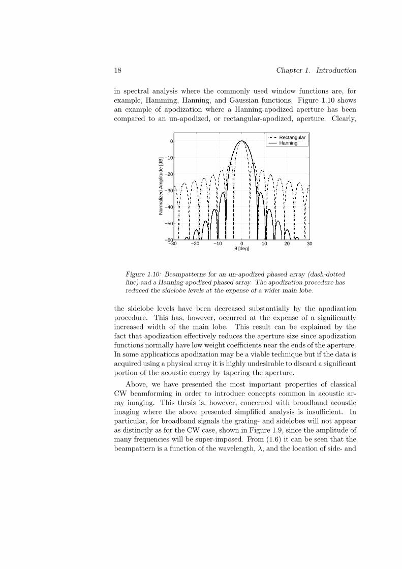
As mentioned above, the sidelobe levels can be controlled by performing asmooth apodization of the aperture. This is a technique known as windowing
18 Chapter 1. Introduction
in spectral analysis where the commonly used window functions are, forexample, Hamming, Hanning, and Gaussian functions. Figure 1.10 showsan example of apodization where a Hanning-apodized aperture has beencompared to an un-apodized, or rectangular-apodized, aperture. Clearly,
−30 −20 −10 0 10 20 30−60
−50
−40
−30
−20
−10
0
θ [deg]
Nor
mal
ized
Am
plitu
de [d
B]
RectangularHanning
Figure 1.10: Beampatterns for an un-apodized phased array (dash-dottedline) and a Hanning-apodized phased array. The apodization procedure hasreduced the sidelobe levels at the expense of a wider main lobe.
the sidelobe levels have been decreased substantially by the apodizationprocedure. This has, however, occurred at the expense of a significantlyincreased width of the main lobe. This result can be explained by thefact that apodization effectively reduces the aperture size since apodizationfunctions normally have low weight coefficients near the ends of the aperture.In some applications apodization may be a viable technique but if the data isacquired using a physical array it is highly undesirable to discard a significantportion of the acoustic energy by tapering the aperture.
Above, we have presented the most important properties of classicalCW beamforming in order to introduce concepts common in acoustic ar-ray imaging. This thesis is, however, concerned with broadband acousticimaging where the above presented simplified analysis is insufficient. Inparticular, for broadband signals the grating- and sidelobes will not appearas distinctly as for the CW case, shown in Figure 1.9, since the amplitude ofmany frequencies will be super-imposed. From (1.6) it can be seen that thebeampattern is a function of the wavelength, λ, and the location of side- and

1.2. Conventional Array Imaging 19
grating lobes will, therefore, change with frequency. Thus, super-imposingthe amplitude of many frequencies will smoothen the beampattern [9].
Furthermore, classical array imaging has many deficiencies that limit itsusefulness, especially for sparse array data. Particular problems associatedwith conventional array imaging are:
• The array elements are treated as point sources. That is, the DASoperation does not compensate for the specific diffraction effects dueto finite sized array elements.
• The distance between the array elements, array pitch, must be lessthan half the acoustic wavelength to avoid artifacts from aliased lobes.
• From (1.8) it is apperent that the resolution is determined mainly bythe array aperture. In particular, the lateral resolution is not depen-dent on the quality of the signal, measured for instance by the signal-to-noise ratio (SNR). Nor does the time available for acquiring datainfluence the resolution (see also [4, 17]). This implies that gatheringdata over a longer period of time would not improve lateral resolution.
• The sidelobe levels can only be reduced by tapering or apodizing theaperture which has the cost of a wider main-lobe.
• The range- or temporal resolution is determined by the interrogatingwavelet. This fact was not mentioned in the discussion above, but theinterrogating wavelet is determined by the electro-mechanical proper-ties of the array elements and the driving input signal which resultsin a band-limited waveform. The temporal resolution is then roughlygiven by the length of that waveform [18].
The first two issues above are perhaps the most severe since they imposerestrictions on the array design, that is: 1) the element size must be small incomparison to the acoustical wavelength and, 2) the array sampling theoremlimits of the array pitch. It is of great interest to relax these two restrictionssince this will allow for larger sized array elements, capable of transmittingmore acoustic power, as well as sparse array designs.
In many medical and NDE applications, where the available aperturesare only a few tens of wavelengths and the F -numbers are in the order ofunity or more, the resolution achieved using classical beamforming is ratherlimited. It is, therefore, desirable to develop reconstruction algorithms that
20 Chapter 1. Introduction
are not restricted by the Rayleigh limit (1.8).5
Classical beamforming using apodization is today, essentially, a reminis-cence from the past when high-resolution imaging was performed by usinglenses. When fast computers are available beamforming in its classical formis not any longer optimal in any sense of optimal information processing
and as E.T. Jaynes stated [29]: “once one is committed to using a com-puter to analyze the data, the high-resolution imaging problem is completelychanged”. The E.T. Jaynes’ paper is concerned with optical imaging butthe results are equally applicable to acoustic imaging. The conclusion fromthis paper is nicely summarized by:
1. Keep your optical system clear and open, gathering themaximum possible amount of light (i.e., information).
2. Don’t worry about wiggles in the point-spread function; thecomputer will straighten them out far better than apodiza-tion could ever have done, at a small fraction of the cost.
3. For the computer to do this job well, it needs only to knowthe actual point-spread function G(x), whatever it is. Soget the best measurement of G(x) that you can, and let thecomputer worry about it from then on.
4. What is important to the computer is not the spatial ex-tent of the point-spread function, but its extent in Fouriertransform space; over how large “window” in k-space doesthe PSF give signals above the noise level, thus deliver-ing relevant information to the computer? Apodizing con-tracts this window by denying us information in high spa-tial frequencies, associated with the sharp edge of the pupilfunction. But this is just the information most crucial forresolving fine detail! In throwing away information, it isthrowing away resolution. Apodization does indeed “re-move the foot;” but it does it by shooting yourself in thefoot.
Translated to acoustical imaging this means that one should transmit as
5Resolution improvement beyond the Rayleigh limit, is often referred to as super-
resolution or wavefield extrapolation [17]. Super-resolution has been the topic for intensiveresearch in both electromagnetic and acoustic imaging [19–28].

1.3. Problem Formulation 21
much acoustic energy as possible in all directions6 in order to maximize thesignal-to-noise ratio and then let the computer compensate for interrogatedwaveforms and diffraction effects.
Our approach which is discussed in more detail in the next section willfollow to E.T. Jaynes’ suggestions.
1.3 Problem Formulation
The general objective of array imaging, that is, extracting information onthe scattering strength of an object under study is, as discussed above,traditionally performed using beamforming. The need for new and morepowerful imaging methods is due to the unsatisfactory performance of thetraditional DAS beamforming observed especially in the near field.
In the approach presented here the imaging problem is formulated as animage reconstruction problem. The basic idea is to create a model of theimaging system that describes the wave propagation and all other proper-ties of the array system with sufficient accuracy compensate for the imagedegradation introduced by the array system. Problems of this type, knownas inverse problems, often require a sophisticated mathematical tools toobtain a satisfactory solution. This is particularly evident for noisy and in-complete data. In particular, when pursuing image reconstruction one mustbear in mind that [31]:
• Obtaining true solutions from the imperfect data is impossible.
• Computational and methodological complexity has to be balancedagainst the quality of the results.
The first issue is related to the fact that the reconstruction performancedepends on the amount of information or evidence that is available. Thatis, the reconstruction performance is directly related to the available back-ground information regarding the scatterers and the imaging system as wellas the evidence contained in the data. In particular, if the model does notfit the data well, then the reconstruction performance will be poor, even ifthe data is almost noise free. On the other hand, an excellent reconstruc-tion performance can be obtained, even for very noisy data, if a strong a
priori information of the scattering amplitudes is available. An optimal
6In medical applications upper limits on average pressure amplitude is often imposedto avoid damage and pain to the patient [30].

22 Chapter 1. Introduction
strategy should, therefore, properly process both the prior information andthe information contained in the data.
The second issue is due to the practical reality: the computational ca-pacity and the available memory resources are limited, which requires com-promises in the design of the reconstruction algorithm. The reconstructionalgorithms discussed in this thesis are more computationally demandingthan classical beamforming but all the algorithms have been implementedon as-of-today standard PC hardware.
As pointed out above, it is vital for the reconstruction performance thatboth the model is accurate and the reconstruction algorithm makes use ofall the available information. These two topics are discussed further below.
1.3.1 The Image Formation Model
The array imaging system has been modeled as a linear time-invariant (LTI)system. Such a system can be modeled using convolutions of the array inputsignals and the impulse responses corresponding to each array element andobservation point. However, it should be emphasized that, even if the systemis time-invariant it is in general not position invariant. That is, the impulseresponses, corresponding to each array element are functions of the positionof the observation point.
To simplify the discussion we consider a pulse-echo measurement usinga single array element. Furthermore, we consider scattering from a singlescatterer at observation point r. The scatterer is assumed to have a scat-tering strength o(r). The received signal, uo(k), can then be modeled as anoise corrupted convolution
uo(t) = o(r)h(r, t) ∗ ui(t) + e(t), (1.9)
where h(r, t) is the double-path impulse response of the overall ultrasonicsystem, ui(t) is the input signal driving the transducer element and, e(t)is the noise.7 In order to obtain an accurate model for broadband arrayimaging the impulse response, h(r, t), must account for both the diffrac-tion effects associated with the transducer element and the electro-acousticproperties of the transducer. The impulse responses are therefore generallyspatially variant.
7The “noise” term describes everything that is observed in the data that can not bepredicted by the linear model. There is no judgment made whether the error is “random”or “systematic”. It can, however, be understood that the noise term is a combination ofmodeling errors and thermal measurement noise.

1.3. Problem Formulation 23
To obtain a model useful for array imaging it is not sufficient to con-sider only a single observation point. If we confine our model to be linear,then (1.9) can easily be extended by summing contributions from many ob-servation points in a suitable region. Throughout this thesis it is assumedthat the scatterer’s locations are known approximately so that a ROI canbe defined within the medium, or specimen, before any experiments areconducted.
Note that if the imaging system is properly modeled all scatterers illu-minated by the incident field are confined within the ROI. Otherwise, thefields originating from the scatterers outside the ROI may cause large mod-eling errors. In particular, it is impossible for the reconstruction algorithmto map the scatterers outside the ROI to the correct location.
The single A-scan model can now be extended to include several elementsor transducer positions. The extended discretized model can be expressedas
y =
y0
y1...
yL−1
= Po + e
=
Pd(0,0) Pd(1,0) · · · Pd(N−1,0)
Pd(1,0) Pd(1,1) · · · Pd(N−1,1)...
......
Pd(0,L−1) Pd(1,L−1) · · · Pd(N−1,L−1)
o0
o1...
oN−1
+
e0
e1...
eL−1
(1.10)
where
yn =[
hd(n,n)0 h
d(n,n)1 · · · h
d(n,n)M−1
]
(O)0,n
(O)1,n...
(O)M−1,n
= Pd(n,n)on. (1.11)
The vector yn is the A-scan acquired using a transducer at (xn, 0), hd(n,n)m is
the discrete-time system impulse response corresponding to the observationpoint (xn, zm) for the nth transducer position, o is the vectorized scatteringimage, and e is the noise vector. The model (1.10) is described in detailin Chapter 4. The propagation matrix, P, contains the impulse responsesfor all observation points to the corresponding array elements. Thus, themodel (1.10) is a fully spatial variant model of the imaging system.

24 Chapter 1. Introduction
The benefit of using a spatial variant model, compared to a spatial in-
variant approximations, is that the model is equally valid in the near-fieldas in the far-field of the aperture.8 A reconstruction method based on themodel, (1.10), should therefore be applicable both in the near- and the far-field.
1.4 Thesis Contributions and Relation to Earlier
Work
Ultrasonic imaging has been an active research area for at least 40 years [32].A substantial part of that research has been on ultrasonic array imagingand beamforming. A considerable effort has been spent to improve thebeamforming performance. Here, we present a selection of previous researchrelated to the array imaging problem treated in this thesis.
The previous efforts can roughly be categorized as 1D and 2D process-ing methods. The 1D methods aim at improving the temporal or rangeresolution in conventional beamforming. Two common approaches are:
Pulse compression: In synthetic aperture radar (SAR) and synthetic aper-ture sonar (SAS) applications, the incoming echos are usually time-or range-compressed by correlating them with the transmitted wave-form [33–35]. If the correlation pattern has a sharp peak, then thetemporal resolution is increased. In SAS frequency sweeped so-calledchirp signals are often used, and it usually results in a sharp correlationpattern [36].
1D Deconvolution: In medical and NDT applications it is most commonto use broadband pulse excitation and the pulse shape is thereforemainly determined by the electro-mechanical properties of the usedtransducer. In this case pulse compression will in general not improvetemporal resolution much. For these applications 1D deconvolutiontechniques can be utilized to improve temporal resolution [37, 38].
Various 2D methods have been utilized to improve both temporal andlateral resolution. Two examples are:
8The drawback of using a spatial variant model is the rather large amount of computermemory that is required to store all impulse responses.

1.4. Thesis Contributions and Relation to Earlier Work 25
2D Deconvolution with spatial invariant kernels: 2D deconvolutionmethods have been applied to ultrasonic array imaging where the for-ward problem has been approximated using a spatial invariant convo-lution kernel to allow standard Wiener filtering techniques [39–42].
Inverse filtering methods: Inverse filtering methods have recently beenapplied to acoustic imaging. In these methods a deterministic ap-proach is taken and the inverse is found by means of singular valuedecomposition techniques [43–45].
In addition to the approaches presented above, Bayesian linear minimummean squared error (MMSE) methods have been applied to ultrasonic arrayimaging, but only for narrow band signals and for simplified models that donot consider the array element size [21–23].
However, no reports on methods using a fully spatial variant model thatuse a realistic model for finite-sized transducers has been presented so far.
Thesis Contribution
An important contribution of this thesis is a new approach to ultrasonicimaging which incorporates the time-domain ultrasonic model of the imagingsystem into the Bayesian estimation framework. The most commonly usedapproach to ultrasonic imaging involves the design of focusing and steeringultrasonic beams using discrete-time focusing laws applied to finite-sizedtransducers. This approach, which is inspired by geometrical optics, aims atcreating analogues of lens systems using ultrasonic array systems. Althoughformal solutions treating imaging as a deterministic inverse problem havebeen proposed before, see for example, [43, 45], presenting the ultrasonicimaging as an estimation problem and solving it using a realistic discrete-time model is new.
The contributions of this thesis is described in more detail next.
Model: A linear discrete-time matrix model of the imaging system takinginto account model uncertainties has been developed.
Problem Statement: A new approach to ultrasonic imaging has been pro-posed. It globally optimizes the imaging performance taking into ac-count parameters of the imaging system and the information about the

26 Chapter 1. Introduction
ROI and errors known a priori.9 The proposed approach is more gen-eral than the traditional imaging methods that maximize the signal-to-noise ratio for a certain point in the ROI using a simplified geometricaloptics model of the imaging system.
Solution: Estimation of the scattering strengths has been performed us-ing tools from Bayesian estimation theory. The imaging can be seenas extracting information about the targets in ROI contained in themeasurements performed using the imaging setup in presence of mea-surement errors.
Special Cases: A linear MMSE filter is derived, as a special case of theproposed approach, using Gaussian measurement noise and a Gaussianprobability density function (PDF) for the scatterers in the ROI. Thelinear MMSE solution takes the form of a spatio-temporal filter whichdeconvolves the distortion caused by the transducer diffraction effectsin the ROI using the information contained in the transducer’s spatialimpulse responses (SIRs). Furthermore, a non-linear (maximum a pos-teriori) MAP estimator is proposed for imaging targets with positivescattering strengths.
Experiments: The new imaging algorithms have been used on simulatedand real ultrasonic data. The algorithms have been applied to mono-static synthetic aperture imaging as well as to parallel array imaging.
Parts of the results presented in this thesis have been published in thefollowing papers:
• F. Lingvall“A Method of Improving Overall Resolution in Ultrasonic Array Imag-ing using Spatio-Temporal Deconvolution” Ultrasonics, Volume 42, pp.961–968, April 2004.
• F. Lingvall, T. Olofsson and T. Stepinski“Synthetic Aperture Imaging using Sources with Finite Aperture—Deconvolution of the Spatial Impulse Response”, Journal of the Acous-tic Society of America, JASA, vol. 114 (1), July 2003, pp. 225-234.
• F. Lingvall and T. Stepinski“Compensating Transducer Diffraction Effects in Synthetic Aperture
9Optimization of the input signals driving the array elements are not considered in thiswork.

1.5. Outline of the Thesis 27
Imaging for Immersed Solids”, IEEE International Ultrasonic Sympo-sium, October 8-11, Munich, Germany, 2002.
• F. Lingvall, T. Olofsson, E. Wennerstrom and T. Stepinski“Optimal Linear Receive Beamformer for Ultrasonic Imaging in NDE”,Presented at the 6th World Congress of NDT, Montreal, August, 2004.
• T. Stepinski and F. Lingvall“Optimized Algorithm for Synthetic Aperture Imaging”, Presented atthe IEEE International Ultrasonic Symposium, 24–27 August, Montreal,Canada, 2004.
1.5 Outline of the Thesis
The thesis is divided in three major parts: Ultrasound Theory and Model-
ing, Methods based on Delay-and-Sum Focusing, and Bayesian Ultrasonic
Image Reconstruction. The first part consists of Chapters 2–4, where Chap-ter 2 and 3 include a comprehensive introduction to acoustic wave propaga-tion theory and the impulse response method, whereupon the discrete-timemodel, presented in Chapter 4, is based on. The second part consists ofChapter 5 and 6 where classical array imaging is treated and, in particular,the broadband properties are discussed. These methods are then used asbenchmarks for the Bayesian reconstruction methods presented in the lastpart, consisting of Chapters 7 and 8.
Chapter 2: Ultrasound Wave Propagation
In this chapter we present the time domain model used for modeling thetransducer radiation process in this thesis. This chapter gives a comprehen-sive introduction to time domain acoustic modeling for anyone working inthe interdisciplinary field of ultrasonic signal processing. Here, the wavepropagation phenomena are expressed using a convolutional formulationwhich should be familiar to people working with signal processing. Thischapter also includes the definition of the spatial impulse response whichplays a central role in the impulse response method.

28 Chapter 1. Introduction
Chapter 3: The Spatial Impulse Response
Here the spatial impulse response (SIR) concept is studied in more detail.In particular, the role of the SIRs as a spatial variant filter is discussed.Situations where the spatial impulse responses can be computed analyticallyis reviewed. The approach that is used to sample analytical SIRs is alsopresented. Moreover it also includes a description of the numerical methodused for situations when no analytical solutions can be found. For suchsituations the author has developed software tool which is described at theend of the chapter.
Chapter 4: A Discrete Linear Model for Ultrasonic Imaging
This chapter presents the spatial variant discrete model which constitutesthe basis for the Bayesian reconstruction methods utilized in this thesis.We describe the modeling of the combined transmission, reception, and thescattering processes. The model is expressed using a matrix formalism whichfacilitates the derivation of the reconstruction algorithms presented in thelast part of the thesis.
Chapter 5: The Synthetic Aperture Focusing Technique
The synthetic aperture focusing technique is a widespread method used inultrasonic array imaging. This chapter reviews the basic properties of themethod with a focus on broadband characteristics and the specific diffractioneffects of finite sized transducers.
Chapter 6: Real Aperture Array Beamforming
This chapter presents some aspects of real aperture array imaging, that is,array imaging with physical arrays. In particular the effects that finite sizedarray elements have on the transmitted acoustic field is discussed. Thischapter also introduces the concept of parallel array imaging.
Chapter 7: Ultrasonic Image Reconstruction Methods
The proposed novel Bayesian reconstruction methods for ultrasonic arrayimaging is introduced here. The chapter also contains a comparison of the

1.6. Financial Support 29
Bayesian methods with common methods for solving so-called ill-posed in-verse problems.
Chapter 8: Applications
The aim of this chapter is to report results of experiments and simulations forboth synthetic and real array apertures, comparing the Bayesian estimatorspresented in Chapter 7 with conventional beamforming methods. Aspectstreated include the size effects of finite-sized transducers, sparse sampled orunder-sampled arrays, as well as parallel array imaging.
Chapter 9: Performance of the Optimal Linear Estimator
The aim of this chapter is to show that Bayesian analysis constitute a usefultool for designing and evaluating ultrasonic array systems. This is due tothe fact that Bayesian methods provide a measure of the accuracy of theestimates.
Chapter 10: Summary and Future Work
Here conclusions are drawn and directions for future research are indicated.
1.6 Financial Support
We gratefully acknowledge the financial support obtained from the SwedishNuclear Fuel and Waste Management Co. (SKB).

30 Chapter 1. Introduction

Part I
Ultrasound Theory and
Modeling
31


CHAPTER 2
Ultrasound Wave Propagation
THIS thesis is concerned with acoustic array signal processing and forthat purpose a model of the acoustic array imaging sytem is needed. In
particular, the transmission, propagation, scattering as well as the receptionprocesses must be modeled. The purpose of acoustic wave modeling is tocalculate the acoustic field in a medium given the field sources, geometry, andthe initial and boundary conditions of the problem. This typically involvesfinding a solution to the wave equation. As mentioned in Chapter 1, onlylongitudinal waves are considered in this thesis, and longitudinal waves, bothin fluids and solids, are well described by the linear acoustic wave equation.1
This chapter is concerned with modeling the transmission and propaga-tion processes or, in other words, the acoustic radiation process of an ul-trasonic transducer. The scattering and reception process will be discussedlater in Chapter 4. It will be shown here that the pressure at an observa-tion point can be expressed as a convolution between the normal velocityon the transducer surface and an impulse response that is determined bythe geometry of the transducer and the boundary conditions. This impulseresponse, known as the spatial impulse resonse (SIR), is the foundation of
1Linear wave propagation describes many acoustic phenomena surprisingly well. Wavepropagation in a fluid will be nearly linear if the fluid is uniform and in equilibrium, andthe viscosity and thermal conduction can be neglected, as well as if the acoustic pressuregenerated by a transducer is small compared to the equilibrium pressure [46]. In ultrasonicarray imaging linear wave propagation is normally assumed which also is the case in thisthesis.
33

34 Chapter 2. Ultrasound Wave Propagation
the ultrasonic wave modeling performed here.
The chapter is organized as follows: The acoustic wave equation is intro-duced in Section 2.1, and Section 2.2 reviews the method of Green’s functionsfor finding solutions to the wave equation. Particlar solutions, given by theinitial and boundary conditions, are discussed in Section 2.3. The presentedsolutions take the form of three integral expressions that correspond to, therigid baffel, the soft baffle, and the free-space boundary conditions, respec-tively. All these integral formulas can be expressed in a convolutional formwhich is attractive since wave propagation can now be modeled using lin-ear systems theory. In Section 2.4 it is finally shown how the sound fieldcan be explicitly expressed as convolutions between the transducer’s normalvelocity and the SIRs.
2.1 The Acoustic Wave Equation
Wave propagation in an isotropic compressible medium containing an acous-tic source can be described by the acoustic wave equation [46],
∇2p(r, t) − 1
c2p
∂2
∂t2p(r, t) = fp(r, t), (2.1)
where the scalar function, p(r, t) is the pressure at r and time t, cp is thesound speed of the medium, and fp(r, t) is the source density, or the drivingfunction of the source. The wave equation can also be expressed in terms ofa velocity potential φ(r, t),
∇2φ(r, t) − 1
c2p
∂2
∂t2φ(r, t) = fφ(r, t). (2.2)
The pressure and the potential is related through,
p(r, t) = ρ0∂φ(r, t)
∂t, (2.3)
and ρ0 is the equilibrium density of the medium which is assumed to beconstant.
The wave equation (2.1) describes the wave propagation in space andtime for a driving function fp(r, t). The driving function can be seen as theinput signal to the acoustical system, and a solution to the wave equationis the response in space and time for that input signal.

2.2. Green’s Functions 35
Here we are interested in obtaining a solution where the input signalis the normal velocity on the active area of the transducer. An analythicalsolution to the wave equation is in general difficult to obtain except for somespecial cases. Fortunately, a piezoelectric transducer can be well describedas a rigid piston due to the large difference in acoustic impedance betweenthe piezoelectric material and the medium (water). Under such conditions, asolution can be found by the method of Green’s functions which is discussedin the next section.
2.2 Green’s Functions
In the theory of linear time-invariant systems, the impulse response of asystem fully describes its properties. Green’s function has an analogousproperty for the wave equation. To see this, let us first introduce the differ-ential operator,
L = ∇2 − 1
c2p
∂2
∂t2. (2.4)
The wave equation (2.1) can then be expressed as
Lp(r, t) = fp(r, t). (2.5)
Since L is a differential operator, the inverse operator must be an integraloperator. Green’s function is the kernel for this integral operator. Physi-cally Green’s function is the solution to a linear partial differential equation(PDE) for a unit impulse disturbance [47]. Here the PDE is the wave equa-tion, (2.1), which becomes,
∇2g(r − r0, t − t0) −1
c2p
∂2
∂t2g(r − r0, t − t0) = δ(r − r0, t − t0) (2.6)
for a unit impulse source, δ(r, t), at r0 applied at time t0. If g(r − r0, t −t0) is known for the problem given by (2.1) and the boundary- and initialconditions, the solution for an arbitrary source fp(r, t) can be obtained bythe following procedure:
First, multiply (2.1) with g(r, t), and (2.6) with p(r, t), and then thesubstract the results, to obtain,
g(r − r0, t − t0)∇2p(r, t) − p(r, t)∇2g(r − r0, t − t0)
= p(r, t)δ(r − r0, t − t0) − g(r − r0, t − t0)f(r, t).(2.7)

36 Chapter 2. Ultrasound Wave Propagation
Interchange r with r0 and t with t0, and integrate with respect to t0 andr0 over time and the volume V defining our region-of-interest and use thesifting property of the delta function. We thus obtain, [48]
∫ t+
−∞
∫
V
(
g(r − r0, t − t0)∇2φ(r0, t0) − p(r0, t0)∇2g(r − r0, t − t0)
)
dr0 dt0
= p(r, t) −∫ t+
−∞
∫
Vg(r − r0, t − t0)f(r0, t0)dr0 dt0,
(2.8)
where the notation t+ means t+ε, for an arbitrary small ε, thereby avoidingan integration ending at the peak of a delta function.
Now, by using Green’s theorem [17], stating that two functions, u(r, t)and v(r, t), with continous first and second order partial derivatives (within,and on a surface S inclosing a volume V ) are related through
∫
V
(u(r, t)∇2vn(r, t) − vn(r, t)∇2u(r, t)
)dr
=
∫
S
(
u(r, t)∂vn(r, t)
∂n− vn(r, t)
∂u(r, t)
∂n
)
dS,
(2.9)
the volume integral on the left hand side of (2.8) can be turned into a surfaceintegral so that the pressure, p(r, t), can be found to be
p(r, t) =
∫ t+
−∞
∫
Vg(r − r0, t − t0)fp(r0, t0)dr0 dt0+
∫ t+
−∞
∫
S
(
g(r − r0, t − t0)∂
∂np(r0, t0)
− p(r0, t0)∂
∂ng(r − r0, t − t0)
)
dS dt0.
(2.10)
Here n is the outward normal on S. Eq. (2.10) is an integral operator thatexpresses the pressure at r both for a source within the volume V and onthe surface of V .
When modeling the acoustic radiation from an ultrasonic transducer thesource, i.e., the transducer, is located on S and and the source term inside Vis then not present, fp(r, t) = 0. Eq. (2.10) then reduces to the time-domain

2.3. Boundary Conditions and Related Integrals 37
Helmholtz-Kirchhoff, or the Helmholtz equation
p(r, t) =
∫ t+
−∞
∫
S
(
p(r0, t0)∂g(r − r0, t − t0)
∂n
− g(r − r0, t − t0)∂p(r0, t0)
∂n
)
dS dt0.
(2.11)
To obtain an expression for the pressure waveform in the transmit processwe need to consider the initial- and boundary conditions which are discussednext.
2.3 Boundary Conditions and Related Integrals
The Helmholtz equation (2.11) may have different forms for different bound-ary conditions. The Rayleigh integral, the Rayleigh-Sommerfeld integral,and the Kirchhoff integral are three forms for three different boundary con-ditions that we will considered here.
2.3.1 The Rayleigh Integral
The boundary conditions determine the impulse response, i.e., Green’s func-tion, for the problem at hand. If a point source is in free space, then theradiated waves will spread spherically and g(r − r0, t − t0) is given by thefree-space Green’s function [46]
gf(r − r0, t − t0) =δ (t − t0 − |r − r0|/cp)
4π|r − r0|, (2.12)
where the super-script, F, denotes free-space conditions.
If some part of S is rigid, then the normal derivative of the pressure onthat part of the boundary is zero. A wave can now be reflected by the rigid,or hard, boundary so the pressure at r, from a source at r0, is for a planarboundary, the sum of two spherical waves: the direct and the reflected wave,see Figure 2.1. Green’s function then becomes
gh(r − r0, t − t0) =δ (t − t0 − |r − r0|/cp)
4π|r − ro|+
δ (t − t0 − |r − r′0|/cp)
4π|r − r′0|,
(2.13)
where the super-script, H, denotes hard or rigid boundary conditions.

38 Chapter 2. Ultrasound Wave Propagation
r‘0
r0
r
Rig
id B
ou
nd
ary
Direct Wave
Reflected Wave
Figure 2.1: Illustration of a wave reflected by a rigid boundary for a sourceat r0.
If the boundary is located in the xy-plane the point r′0 = (x0, y0,−z0) isthen the mirror point of r0. On the boundary, z0 = 0, the normal derivativeof Green’s function (2.13) vanishes, hence the contribution from the rigidplane to the surface integral in (2.11) will be zero and (2.13) becomes
gh(r − r0, t − t0) =δ (t − t0 − |r − r0|/cp)
2π|r − ro|= 2gf(r − r0, t − t0), (2.14)
with∂
∂ngh(r − r0, t − t0) = 0. (2.15)
Now, if the source, i.e., the transducer, is located in the rigid plane, oftenreferred to as the rigid baffle as illustrated in Figure 2.2, then the baffle (Sb)will not contribute to the field.
By using the Sommerfeld radiation condition, where one lets the volumeV expand to infinity, the contributions from the remaining part of the surface(depicted
∑in Figure 2.2) will cancel [17]. Thus, the only area that will
contribute to the surface integral is the active area of the transducer. Ifthe transducer is planar, then the wave in the vicinity will also be planar,resulting in that the normal derivative of the pressure, its time derivative,and the time derivative of the source velocity will be proportional [9, 49]
∂p(r0, t)
∂n= − 1
cp
∂p(r0, t)
∂t= −ρ0
∂
∂tvn(r0, t). (2.16)
Substituting (2.16) and (2.14) into (2.11) results in the well known Rayleigh
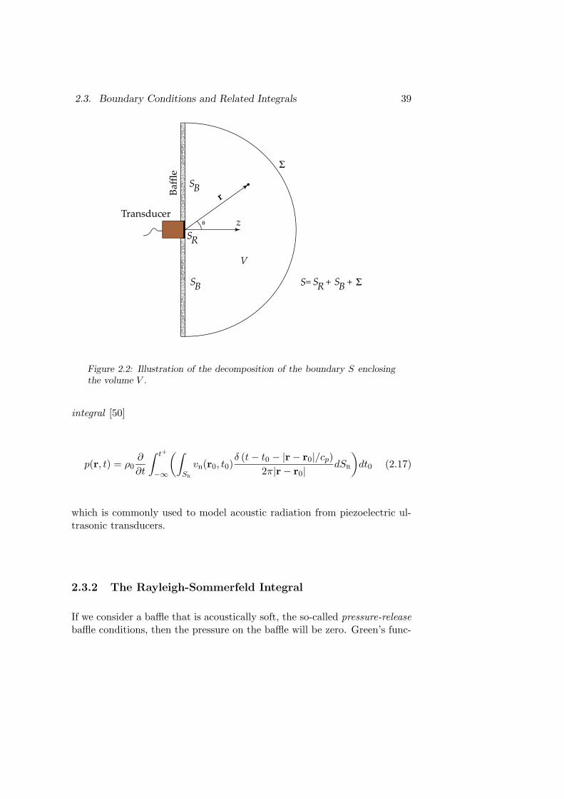
2.3. Boundary Conditions and Related Integrals 39
Baffle
Transducer
SR
SB
SB
Σ
z
V
S= + + Σ
SR
SB
r
θ
Figure 2.2: Illustration of the decomposition of the boundary S enclosingthe volume V .
integral [50]
p(r, t) = ρ0∂
∂t
∫ t+
−∞
(∫
Sr
vn(r0, t0)δ (t − t0 − |r − r0|/cp)
2π|r − r0|dSr
)
dt0 (2.17)
which is commonly used to model acoustic radiation from piezoelectric ul-trasonic transducers.
2.3.2 The Rayleigh-Sommerfeld Integral
If we consider a baffle that is acoustically soft, the so-called pressure-release
baffle conditions, then the pressure on the baffle will be zero. Green’s func-

40 Chapter 2. Ultrasound Wave Propagation
tion and its normal derivative on the baffle (r′0 = r0) will then be 2
gs(r − r0, t − t0) =δ (t − t0 − |r − r0|/cp)
4π|r − ro|− δ (t − t0 − |r − r′0|/cp)
4π|r − r′0|= 0
∂
∂ngs(r − r0, t − t0) ≈
δ′ (t − t0 − |r − r0|/cp)
4πcp|r − r0|2 cos(θ)
(2.18)
where θ is the angle between the normal vector n and r − r0 and δ′(·)is the first derivative of the delta function.3 By substituting (2.18) andp(ro, t) = 0 into (2.11), the Helmholtz equation reduces to the Rayleigh-
Sommerfeld integral formula
p(r, t) = ρ0∂
∂t
∫ t+
−∞
(∫
Sr
vn(r0, t0)δ (t − t0 − |r − r0|/cp)
4π|r − r0|2 cos(θ)dSr
)
dt0.
(2.19)
2.3.3 The Kirchhhoff Integral
For the free-space case, none of the terms in the Helmholtz equation disap-pears and the normal derivative at the plane source of the free-space Green’sfunction becomes
∂
∂ngs(r − r0, t − t0) ≈
δ′ (t − t0 − |r − r0|/cp)
4πcp|r − r0|cos(θ), (2.20)
where the super-script, S, denotes soft boundary conditions. Substitutingthe free-space Green’s function and its derivative (2.20) into Helmholtz equa-tion results in the Kirchhoff integral formula
p(r, t) = ρ0∂
∂t
∫ t+
−∞
(∫
Sr
vn(r0, t0)δ (t − t0 − |r − r0|/cp)
4π|r − r0|(1−cos(θ))dSr
)
dt0.
(2.21)
In summary, by comparing (2.17), (2.19), and (2.21) tha difference be-tween the three different boundary conditions is a direction dependent co-efficient, α(θ), which is (1 − cos(θ)) for the free-space conditions, 2 cos(θ)for the soft baffle, and a constant 2 for the hard baffle. The angular de-pendence of the direction coefficient is shown in Figure 2.3. Normally the
2The approximation for the normal derivative of Green’s function is valid for |r−r0| �λ
2πwhere λ is the wavelength corresponding to the highest frequency in the frequency band

2.4. The Convolution Integral 41
0 1 2 3 4−2.5
−2
−1.5
−1
−0.5
0
0.5
1
1.5
2
2.5
z
x
Free−spaceSoftHard
(a) Polar diagram.
−3 −2 −1 0 1 2 3−20
−15
−10
−5
0
5
10
θ [rad]
Am
plitu
de [d
B]
Free−spaceSoftHard
(b) Directional coefficient as afunction of θ.
Figure 2.3: Angular dependence of the directional coefficient, α(θ), for:a hard baffle α(θ) = 2, a soft baffle α(θ) = 2 cos(θ), and for free-spaceboundary conditions α(θ) = 1 − cos(θ).
hard baffle conditions (i.e., the Rayleigh integral) is used for modeling wavepropagation using an piezoelectric ultrasonic transducer immersed in water.
2.4 The Convolution Integral
In Section 2.3 we found that the Kirchhhoff, Rayleigh, and Rayleigh-So-mmerfeld integrals all shared the form
p(r, t) = ρ0∂
∂t
∫ t+
−∞
(∫
Sr
vn(r0, t0)δ (t − t0 − |r − r0|/cp)
4π|r − r0|α(θ)dSr
)
dt0
(2.22)where α(θ) is the direction coefficient that depends on the boundary condi-tion. If the source velocity is constant over the active area of the transducer(i.e., vn(r0, t0) = vn(t0)), then vn(r0, t0) can be moved outside the surface
of interest [51].3The derivative of a delta function has the property
R ∞
−∞δ′(x)f(x+a)dx = −f ′(a) [48].
42 Chapter 2. Ultrasound Wave Propagation
integral, yielding
p(r, t) = ρ0∂
∂t
∫ t+
−∞vn(t0)
(∫
Sr
δ (t − t0 − |r − r0|/cp)
2π|r − rr|α(θ)dSr
)
dt0
= ρ0∂
∂tvn(t) ∗
(∫
Sr
δ (t − |r − r0|/cp)
2π|r − r0|α(θ)dSr
)
.
(2.23)
Thus, the pressure at r can be expressed as a temporal convolution betweenthe two factors,
ρ0∂
∂tvn(t), (2.24)
and ∫
Sr
δ (t − |r − r0|/cp)
4π|r − r0|α(θ)dSr. (2.25)
The normal velocity, vn(t0), depends on the electro-mechanical transferfunction of the transducer combined, i.e., convolved, with the excitationsignal of the transducer. If the excitation signal is a delta function, then thefactor (2.24) can be seen as the forward electrical impulse response of thetransducer.
The second factor, (2.25), describes the acoustic wave propagation fromthe tranducer surface to the observation point, r. This factor is then theresponse at r that one would obtain for an impulsive transducer surfacevelocity. The factor (2.25) is commonly called the spatial impulse response
(SIR). The spatial impulse response depends of the shape and size of theactive area (Sr) of the transducer, and it is this factor that determines thedirectivity patterns of the transducer. The spatial impulse response has acentral role in this thesis and Chapter 3 is devoted entirely to this issue.
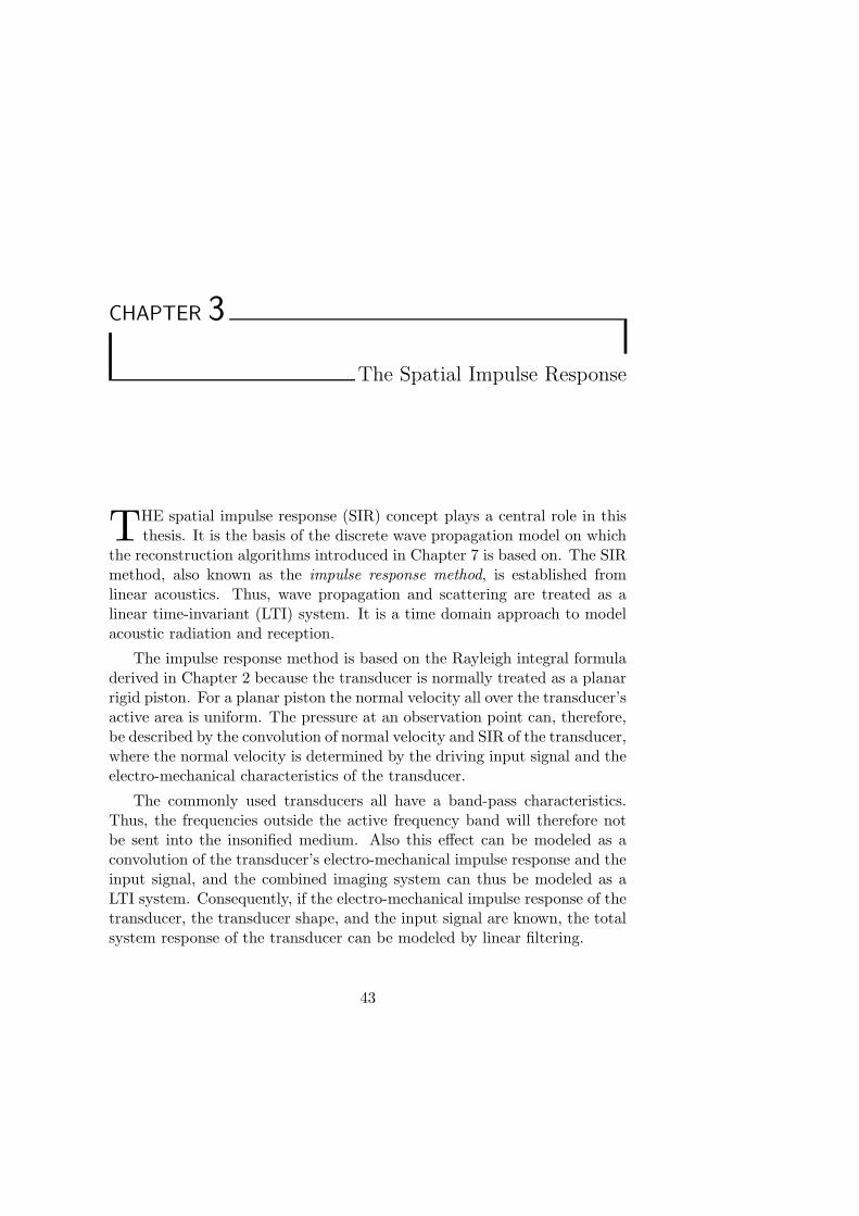
CHAPTER 3
The Spatial Impulse Response
THE spatial impulse response (SIR) concept plays a central role in thisthesis. It is the basis of the discrete wave propagation model on which
the reconstruction algorithms introduced in Chapter 7 is based on. The SIRmethod, also known as the impulse response method, is established fromlinear acoustics. Thus, wave propagation and scattering are treated as alinear time-invariant (LTI) system. It is a time domain approach to modelacoustic radiation and reception.
The impulse response method is based on the Rayleigh integral formuladerived in Chapter 2 because the transducer is normally treated as a planarrigid piston. For a planar piston the normal velocity all over the transducer’sactive area is uniform. The pressure at an observation point can, therefore,be described by the convolution of normal velocity and SIR of the transducer,where the normal velocity is determined by the driving input signal and theelectro-mechanical characteristics of the transducer.
The commonly used transducers all have a band-pass characteristics.Thus, the frequencies outside the active frequency band will therefore notbe sent into the insonified medium. Also this effect can be modeled as aconvolution of the transducer’s electro-mechanical impulse response and theinput signal, and the combined imaging system can thus be modeled as aLTI system. Consequently, if the electro-mechanical impulse response of thetransducer, the transducer shape, and the input signal are known, the totalsystem response of the transducer can be modeled by linear filtering.
43

44 Chapter 3. The Spatial Impulse Response
Evidently, to model the ultrasonic imaging system, the SIRs associatedwith the transducer are needed. Analytical solutions to SIRs exist for a fewgeometries, but one must in general resort to numerical methods. Section 3.1discusses some important cases where analytical solutions do exist. Thesetime continuous solutions are however not practical since all signals acquiredare normally sampled and time discrete models are therefore needed. Sec-tion 3.2 describes the sampling approach of the analytical SIRs used in thisthesis. The total system response is determined by both the electrical im-pulse response and the SIRs. The properties and influence of the electricalimpulse response are discussed in Section 3.3.
As mentioned above, there exist no analytical analytical solutions formany transducer geometries, and in such situation a method based on thediscrete representation (DR) computational concept is used here [52, 53].The DR method is very flexible in the sense that complex transducer shapesas well as arbitrary focusing methods easily can be modeled. Another benefitof the DR method is that the SIRs are directly computed in a discrete form.A short description of the DR method, and a numerical package based onthe DR method that has been developed by the author, is presented in thefinal Section 3.4 of this chapter.
3.1 Analytical Solutions for some Canonical Trans-
ducer Types
In this section a few analytical SIR solutions are presented. These solutionswill be used later in scattering and transducer radiation modeling problems.The first solution considered is the point source that is commonly used inarray imaging. In this thesis, the point source model is mainly used to mod-eling scattering which is discussed in more detail in Chapter 4.1 The otheranalytical solutions considered are the line and the circular disc solutionsthat will be used to model synthetic aperture experiments in Chapters 5and 8.
3.1.1 The Point Source
A point source is a common model used for a source that has an apertureconsiderably smaller than the acoustical wavelength. A point source emits
1In pulse-echo imaging a scatterer can be seen a source of the scattered wave field.

3.1. Analytical Solutions for some Canonical Transducer Types 45
spherical waves, and thus has an angle-independent SIR which is given bythe free-space Green’s function, cf. (2.12),
h(r, t) = seδ (t − |r − rt|/cp)
4π|r − rt|, (3.1)
where rt is the position of the point source and r the position of the observa-tion point. Since the SIR is a delta function the pulse shape will not dependon the observation position, only the pulse’s amplitude will be scaled withthe factor 1/(4π|r− rt|). The scale factor, se in (3.1), is the cross-sectionalarea or the elementary surface of the point source [54]. Note that the ele-mentary surface must be small enough so that the source behaves as a unitpoint source in all aspects except for the scale factor se.
In traditional ultrasonic array imaging, the array elements are treatedas point sources and the total array response is modeled as a superpositionof delayed point source responses. The point source is also commonly usedto model scattering. In this case se is thought of as the cross-section areaof a small scatterer.
3.1.2 The Line Source
A line source, or a uniformly excited line strip, can be used as an approxi-mation of a narrow strip transducer or for modeling scattering from a wiretarget that is commonly used in ultrasonic imaging. Here the line strip,
x
y
z
aa
(a) A line source.
x
y
z
a
(b) A circular disc source.
Figure 3.1: Geometries of a line and a circular disc source.

46 Chapter 3. The Spatial Impulse Response
with length 2a, is assumed to be located on the x-axis, centered at x = 0,see Figure 3.1(a). The SIR of a uniformly excited line strip is given by [55]
for |x| ≤ a,
h(x, z, t) = se ·
0, t < tz
2 1√t2−t2z
, tz < t ≤ t1
1√t2−t2z
, t1 < t ≤ t2
0, t > t2
and for |x| > a,
h(x, z, t) = se ·
0, t ≤ t11√
t2−t2z, t1 < t ≤ t2
0, t > t2
(3.2)
where tz = z/cp is the start time of the SIR when |x| ≤ a and t1,2 =
tz
√
1 +
(
a∓|x|z
)2
. Due to the rotational symmetry of the SIRs for a line
source, only the two-dimensional case is considered here. That is, if theSIRs in the xz-plane are known than all other SIRs can be found by arotation of the plane around the x-axis.2
Note that similar to the point source it is necessary to use a weight, se,for, in this case, the yz-direction cross-sectional area of the line source.
3.1.3 The Circular Disc
Circular transducers are commonly used in ultrasonic imaging applications.Typical examples are NDT/NDE, sonar, and scanned synthetic apertureimaging applications.
The SIR of a circular disc has an analytical solution when the observa-tion point is inside the aperture of the disc,
√
x2 + y2 ≤ a where a is thetransducer radius, and when the observation point is outside the aperture,see Figure 3.1(b) [56]. The disc is assumed to be located in the xy-planecentered at x = y = 0. Let first r denote the distance from the center axis
2The 3D solution for a line source can be found in [49].

3.1. Analytical Solutions for some Canonical Transducer Types 47
of the disc, r =√
x2 + y2, then the disc SIR is given by
for r ≤ a
h(r, t) =
0, t ≤ tz
cp, tz ≤ t ≤ t1cpπ cos−1
(
c2p
t2−t2z+t2r−a/c2p
2tr√
t2−t2z
)
, t1 < t ≤ t2
0, t > t2
for r > a
h(r, t) =
0, t ≤ t1cpπ cos−1
(
c2p
t2−t2z+t2r−a/c2p
2tr√
t2−t2z
)
, t1 < t ≤ t2
0, t > t2
(3.3)
where tz = z/cp is the earliest time that the wave reaches the observation
point r when r ≤ a, tr = r/cp, and t1,2 = tz
√
1 +
(
a∓rz
)2
are the prop-
agation times corresponding to the edges of the disc that are closest andfurtherest away from r, respectively.
Noticeable is that the pulse amplitude of the on-axis SIR is constantregardless of the distance to the observation point.3 The duration of theon-axis SIR is given by t1 = a/cp at z = 0. As the distance increases theduration, t1−tz, of the SIR becomes shorter, and for large z it approaches tothe delta function. The transducer size effects are therefore most pronouncedin the near-field. This is illustrated in Figure 3.2 where the on-axis SIRs atz = 20 and z = 80 mm, respectively are shown. The duration at z = 20 islonger than that of z = 80 and if the distance, z, increases then the on-axisSIR will approach to a delta function, cf. Figures 3.2(a) and (b).
The analytical SIR solutions presented above are the ones that will beutilized in later chapters of this thesis, and additionally, a solution for arectangular transducer is presented in Appendix 3.A.
3The on-axis SIR has duration t1 − tz with the constant amplitude cp in the timeinterval tz ≤ t ≤ t1.

48 Chapter 3. The Spatial Impulse Response
0 5 10 15 20 25 300
200
400
600
800
1000
1200
1400
1600
1800
t [µs]
SIR
Am
plitu
de [m
/s]
(a) Spatial impulse response at z = 20mm.
40 45 50 55 60 65 700
200
400
600
800
1000
1200
1400
1600
1800
t [µs]
SIR
Am
plitu
de [m
/s]
(b) Spatial impulse response at z = 80mm.
Figure 3.2: On-axis spatial impulse responses for a 10 mm disc where thesound speed, cp, was 1500 m/s.
3.2 Sampling Analytical Spatial Impulse Responses
The analytical expressions for the SIRs discussed above must be convertedto a discrete form in order to be useful for digital signal processing. Aproper discrete representation of the SIRs is necessary so that when thesampled SIR is convolved with the normal velocity the resulting waveformcan faithfully represent the sampled measured waveform.
The analytical SIRs have an infinite bandwidth due to the abrupt ampli-tude changes that, for example, could be seen in the line and disc solutionsabove. In some situations the duration of a SIR may even be shorter thanthe sampling interval, Ts, and it is therefore not sufficient to sample theanalytical SIRs by simply taking the amplitude at the sampling instants,tk, since the SIR may actually be zero those time instants. The SIRs arehowever convolved with a band-limited normal velocity, hence the resultingpressure waveform must also be band-limited, cf. (2.23). Consequently, weonly need to sample the SIR in such way that the band-limited recievedA-scans are properly modeled.
Here, the SIR sampling process is performed by collecting all contribu-tions from the continuous time SIR in the corresponding sampling interval[tk −Ts/2, tk +Ts/2]. A discrete version of the a time continuous SIR is then

3.2. Sampling Analytical Spatial Impulse Responses 49
obtained by summing all contributions from the SIR in the actual samplinginterval. That is, the sampled SIR is defined as
h(r, tk) ,1
Ts
∫ tk+Ts/2
tk−Ts/2h(r, t′)dt′. (3.4)
The division by Ts retains the same unit (m/s) of the sampled SIR as thecontinuous one. The amplitude of the sampled SIR, at time tk, is then themean value of the continuous SIR in the corresponding sampling interval,[tk − Ts/2, tk + Ts/2]. Also, as seen from the analytical solutions above, theSIRs always have a finite length as the transducer has a finite size. Thesampled SIRs are therefore naturally represented by finite impulse responsefilters (FIR).
The effect of the sampling scheme (3.4) is illustrated in Figure 3.3 for twodiscs with radii 1.2 and 3 mm, respectively, where the sampling interval, Ts,was 0.04µs. In Figure 3.3(a) the analytic SIR is shorter than the sampling
33.25 33.3 33.35 33.4 33.45 33.50
200
400
600
800
1000
1200
1400
1600
t [µs]
SIR
Am
plitu
de [m
/s]
Sampled SIRAnalytic SIR
(a) Continuous and sampled spatialimpulse responses of a circular discwith radius r = 1.2 mm.
33.25 33.3 33.35 33.4 33.45 33.50
200
400
600
800
1000
1200
1400
1600
t [µs]
SIR
Am
plitu
de [m
/s]
Sampled SIRAnalytic SIR
(b) Continuous and sampled spatialimpulse responses of a circular discwith radius r = 3 mm.
Figure 3.3: Illustration of the spatial impulse response sampling methodused in this thesis. The continuous and sampled on-axis SIRs for two discswith radii 1.2 and 3 mm, respectively are shown where the sampling interval,Ts, was 0.04µs.
interval, Ts. The max amplitude of the discrete SIR is therefore lower thanthen the max amplitude of the continuous SIR. If the duration of the analyticSIR is longer than the sampling interval, as for the 3 mm disc shown in

50 Chapter 3. The Spatial Impulse Response
Figure 3.3(b), then the max amplitudes of the on-axis sampled and analyticdisc SIRs will be the same.
3.3 The Pressure Field
In Chapter 2 it was shown that the pressure waveform at an observationpoint r can be modeled as a convolution of the SIR, h(r, t), correspondingto r with the normal velocity waveform at the transducer surface,
p(r, t) = h(r, t) ∗ v(t). (3.5)
Since all SIRs of practical interest have a low-pass character, there willonly be significant acoustic energy at those observation points where thefrequency-bands of the SIR and the normal velocity overlap. The band-width of the SIR becomes narrower when the observation point is furtheraway the from the center-axis of the aperture because the duration of the SIRgets longer. This makes the beampattern frequency dependent and a trans-ducer with low center frequency has therefore a wider beampattern than atransducer with high center frequency for a fixed size of the transducer.
As an example of this effect, simulation results for two circular disctransducers, with radii r = 1 mm and r = 5 mm respectively, are shownin Figures 3.5 and 3.6. An impulse excitation is used here and the normalvelocity is therefore given by the forward electro-mechanical, or electrical,impulse response of the transducer, that is,
v(t) = hef(t) ∗ δ(t), (3.6)
where hef(t) denotes the transducer’s forward electrical impulse response.The electrical impulse response used here is shown in Figure 3.4, and thecenter frequency is about 3 MHz which corresponds to a wavelength of 0.5mm.4
Figure 3.5 shows the on-axis responses for the two transducer sizes andthe corresponding normalized spectra for the SIRs, the electrical impulseresponse, and the SIRs convolved with the electrical impulse response.
4The electrical impulse response was measured with a Precision Acoustics PVDF hy-drophone. The hydrophone has a bandwidth that is considerably larger than the band-width of the transducer and will, therefore, not affect the measurement of the transducer’selectrical impulse response.
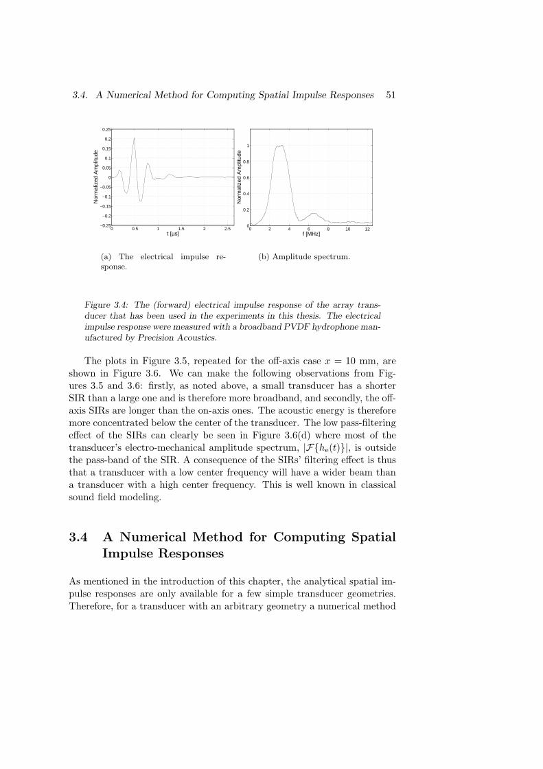
3.4. A Numerical Method for Computing Spatial Impulse Responses 51
0 0.5 1 1.5 2 2.5−0.25
−0.2
−0.15
−0.1
−0.05
0
0.05
0.1
0.15
0.2
0.25
t [µs]
Nor
mal
ized
Am
plitu
de
(a) The electrical impulse re-sponse.
0 2 4 6 8 10 120
0.2
0.4
0.6
0.8
1
f [MHz]N
orm
aliz
ed A
mpl
itude
(b) Amplitude spectrum.
Figure 3.4: The (forward) electrical impulse response of the array trans-ducer that has been used in the experiments in this thesis. The electricalimpulse response were measured with a broadband PVDF hydrophone man-ufactured by Precision Acoustics.
The plots in Figure 3.5, repeated for the off-axis case x = 10 mm, areshown in Figure 3.6. We can make the following observations from Fig-ures 3.5 and 3.6: firstly, as noted above, a small transducer has a shorterSIR than a large one and is therefore more broadband, and secondly, the off-axis SIRs are longer than the on-axis ones. The acoustic energy is thereforemore concentrated below the center of the transducer. The low pass-filteringeffect of the SIRs can clearly be seen in Figure 3.6(d) where most of thetransducer’s electro-mechanical amplitude spectrum, |F{he(t)}|, is outsidethe pass-band of the SIR. A consequence of the SIRs’ filtering effect is thusthat a transducer with a low center frequency will have a wider beam thana transducer with a high center frequency. This is well known in classicalsound field modeling.
3.4 A Numerical Method for Computing Spatial
Impulse Responses
As mentioned in the introduction of this chapter, the analytical spatial im-pulse responses are only available for a few simple transducer geometries.Therefore, for a transducer with an arbitrary geometry a numerical method
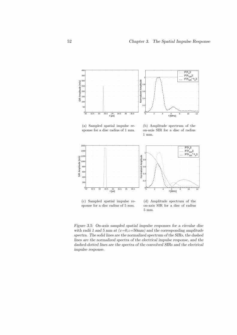
52 Chapter 3. The Spatial Impulse Response
32 32.5 33 33.5 34 34.5 35 35.50
50
100
150
200
250
300
350
400
t [µs]
SIR
Am
plitu
de [m
/s]
(a) Sampled spatial impulse re-sponse for a disc radius of 1 mm.
0 2 4 6 8 10 120
0.2
0.4
0.6
0.8
1
f [MHz]
Nor
mal
ized
Am
plitu
de
|F{he}|
|F{hSIR
}||F{h
SIR* h
e}|
(b) Amplitude spectrum of theon-axis SIR for a disc of radius1 mm.
32 32.5 33 33.5 34 34.5 35 35.50
200
400
600
800
1000
1200
1400
1600
t [µs]
SIR
Am
plitu
de [m
/s]
(c) Sampled spatial impulse re-sponse for a disc radius of 5 mm.
0 2 4 6 8 10 120
0.2
0.4
0.6
0.8
1
f [MHz]
Nor
mal
ized
Am
plitu
de
|F{he}|
|F{hSIR
}||F{h
SIR* h
e}|
(d) Amplitude spectrum of theon-axis SIR for a disc of radius5 mm.
Figure 3.5: On-axis sampled spatial impulse responses for a circular discwith radii 1 and 5 mm at (x=0,z=50mm) and the corresponding amplitudespectra. The solid lines are the normalized spectrum of the SIRs, the dashedlines are the normalized spectra of the electrical impulse response, and thedashed-dotted lines are the spectra of the convolved SIRs and the electricalimpulse response.

3.4. A Numerical Method for Computing Spatial Impulse Responses 53
32 32.5 33 33.5 34 34.5 35 35.50
10
20
30
40
50
60
70
80
90
100
t [µs]
SIR
Am
plitu
de [m
/s]
(a) Sampled spatial impulse re-sponse for a disc radius of 1 mm.
0 2 4 6 8 10 120
0.2
0.4
0.6
0.8
1
f [MHz]
Nor
mal
ized
Am
plitu
de
|F{he}|
|F{hSIR
}||F{h
SIR* h
e}|
(b) Amplitude spectrum of theoff-axis SIR for a disc of radius1 mm.
32 32.5 33 33.5 34 34.5 35 35.50
50
100
150
200
250
300
350
400
t [µs]
SIR
Am
plitu
de [m
/s]
(c) Sampled spatial impulse re-sponse for a disc radius of 5 mm.
0 2 4 6 8 10 120
0.2
0.4
0.6
0.8
1
f [MHz]
Nor
mal
ized
Am
plitu
de
|F{he}|
|F{hSIR
}||F{h
SIR* h
e}|
(d) Amplitude spectrum of theoff-axis SIR for a disc of radius5 mm.
Figure 3.6: Off-axis sampled spatial impulse responses for a circular discwith radii 1 and 5 mm at (x=10 mm,z=50 mm) and the corresponding am-plitude spectra. The solid lines are the normalized spectra of the SIRs, thedashed lines are the normalized spectra of the electrical impulse response,and the dashed-dotted lines are the spectra of the convolved SIRs and theelectrical impulse response.

54 Chapter 3. The Spatial Impulse Response
must be used. The method is used throughout this thesis, the discrete repre-
sentation (DR) method, is based on a discretization of the Rayleigh integralformula, (2.17). In the DR method, the radiating surface is divided intoa set of small surface elements, and the surface integral in the Rayleigh
S
x
y
z
Observation pointrj
j∆
Figure 3.7: Geometry and notations for the discrete representation method.
formula is replaced by a summation, as illustrated in Figure 3.7. The DRmethod facilitates computation of SIRs for non-uniform excitation, apodiza-tion of the aperture, and arbitrary focusing laws since each surface elementcan be assigned a different normal velocity, apdodization or time-delay. TheDR computational concept can therefore be used for computing SIRs for anarbitrary transducer shape or array layout [52, 53].
First, let the total transducer surface be divided into a set of J surfaceelements {∆S0, ∆S1, . . . ,∆SJ−1}. Furthermore, let wj denote an apertureweight, and Rj = |r − rj | the distance from the jth surface element to theobservation point. The discrete SIR can now be approximated by
h(r, tk) =1
2π
J−1∑
j=0
wjδ(tk − Rj/cp − dj)
Rj∆Sj
=J−1∑
j=0
ajδ(tk − Rj/cp − dj),
(3.7)
where dj is a user defined focusing delay and tk = kTs, for k = 0, 1, . . .K−1.The amplitude scaling factor
aj =wj∆Sj
2πRj(3.8)

3.4. A Numerical Method for Computing Spatial Impulse Responses 55
in (3.7) represents the amplitude of the impulse response for an elementarysurface at rj excited by a Dirac pulse, cf. (3.1). Hence, the total responseat time tk is a sum of contributions from those elementary surface elements,∆Sj , whose response arrive in the time interval [tk − Ts/2, tk + Ts/2].
The accuracy of the method depends on the size of the discretization sur-faces ∆Sj . It should however be noted that high frequency numerical noisedue to the surface discretization is in practice not critical since the trans-ducer’s electrical impulse response has a bandwidth in the low frequencyrange (for a further discussion see [53]). Also, these errors are small if theelementary surfaces, ∆Sj , are small. The DR-method is very flexible in thesense that beam steering, focusing, apodization, and non-uniform surfacevelocity can easily be included in the simulation.
The author has developed a software tool, e.g. the DREAM (DiscreteREpresentation Array Modeling) Toolbox, based on the DR method in co-operation with Prof. Bogdan Piwakowski at Lille Groupe � Electronique- Acoustique �, Institut d’Electronique et de Micro-electronique du Nord,France.5 The DREAM toolbox has support for many different transducertypes and array layouts, including arrays with circular, rectangular, andcylindrical focused elements to name a few. Numerical routines from theDREAM toolbox have been used for all the numerical SIR computations inthis thesis when analytical solutions are not available.6
5The DREAM toolbox is available on-line at http://www.signal.uu.se/Toolbox/dream/.6Currently, the DREAM toolbox only has support for computing SIRs in homogeneous
media. In this thesis experiments are performed also using an immersed copper block. Tocompute SIRs for this case an algorithm inspired by the DR method is used which isdescribed in Appendix 3.B.

56 Chapter 3. The Spatial Impulse Response
3.A The Rectangular Source
Rectangular sources are also very common in ultrasonic imaging. Arraytransducers is a typical example where the array elements often have a rect-angular active area.
The analytic SIR for a rectangular transducer can be computed by usingthe solution for an observation point at a corner point under the rectangularaperture, see illustration in Figure 3.8. The solution for the corner point is
x
y
zObservation point
s
l
Figure 3.8: Geometry of a rectangular aperture located in the xy-plane.The y-direction width is given by l and x-direction width by s. Also illus-trated is the location of an observation point located under a corner of therectangular aperture.
given by [57]
h(r, t) =cp
2π
(π
2Π(τ i, τ iv)
− cos−1
(
s
cp
√
t2 − t2z
)
Π(τ ii, τ iv)
− cos−1
(
l
cp
√
t2 − t2z
)
Π(τ iii, τ iv)
)
.
(3.9)
where l is the y-direction width and s the x-direction width of the rectangle.The function Π(·, ·) is the “pulse function” defined as Π(t1, t2) = 1 whent ∈ [t1, t2] and Π(t1, t2) = 0 otherwise. The time delays, τ i, . . . , τ iv, defined

3.A. The Rectangular Source 57
by
τ i = tz
τ ii =√
z2 + s2/cp
τ iii =√
z2 + l2/cp
τ iv =√
z2 + s2 + l2/cp,
(3.10)
are the travel times of the pulse from the four corner points of the rectangleto the observation point, respectively.
The response at an arbitrary observation point can now be obtained byadding and/or subtracting responses from rectangular apertures. There arefour possible cases which are illustrated in Figure 3.9: In Figure 3.9(a) theobservation point is strictly inside the aperture, in Figure 3.9(b) x is outsidethe aperture, in Figure 3.9(c) y is outside the aperture, and in Figure 3.9(d) both x and y is outside the aperture.
For the first case, when the observation point is inside the aperture, theSIR is obtained by summing the contributions from the rectangular sub-apertures I,. . .,IV. When x is outside the aperture the SIR is obtained by firstsumming contributions from the apertures II and III and then subtractingthe two contributions from rectangle I and IV that is not a part of the trueaperture. The SIRs for the two remaining cases are obtained in a similarfashion.
The SIR for the a rectangular aperture can finally be expressed as
h(r, t) =cp
2π
4∑
i=1
gi ·(
π
2Π(τ i
i , τivi )
− cos−1
(
si
cp
√
t2 − t2z
)
Π(τ iii , τ iv
i )
− cos−1
(
li
cp
√
t2 − t2z
)
Π(τ iiii , τ iv
i )
)
(3.11)
where gi = 1 or -1 depends on the location of the observation point.

58 Chapter 3. The Spatial Impulse Response
III
III IV
l1
l4
l3
l2
s1
s2
s4
s3
(a) Both x and y inside the aper-ture.
I
IV
l1
s1
s4
II
III l3
l2
s2
s4
s3
l4
(b) x outside the aperture.
I l1
II
IIIl3
l2
s2
s4
s3
l4
s1
IV
(c) y outside the aperture.
I l1
III l3
s1
II l2
s2
s4
s3
l4
IV
(d) Both x and y outside theaperture.
Figure 3.9: The four possible observation point positions under a rectan-gular aperture. The gray-shaded area denotes the transducer’s active area.

3.B. An Algorithm for Computing SIRs in Immersed Solids 59
3.B An Algorithm for Computing SIRs in Immersed
Solids
One of the experiments presented in Chapter 8 is performed using an im-mersed copper block. To be able to use the model based methods that isintroduced in Chapter 7 we need to compute the SIRs for this setup. Thenumerical method used in this thesis for this case is based on a line sourcemodel with adjustments for the different sound speeds of the two media andthe refraction effects at the water-solid interface, as described below.
Wave propagation in elastic solids are, as mentioned in Chapter 1, morecomplicated than propagation in fluids since many types of waves can prop-agate. In the bulk of the solid both longitudinal and shear waves can prop-agate. The longitudinal and shear waves have different sound speeds wherethe longitudinal sound speed, cCu
p , in copper is around 4600 m/s and the
shear wave sound speed, cCus , is 2250 m/s. Thus, longitudinal waves in
copper travels roughly two times faster than shear waves.
As also mentioned in Chapter 1, mode conversion occurs at interfaceswere the acoustical impedance changes abruptly, resulting in both longi-tudinal and shear wave components. In order to successfully model wavepropagation in an immersed copper block these mode conversion must betaken into account.
To model the wave propagation, at the water-copper interface, considera harmonic plane wave impinging on the interface. The incident longitudinalwave will both be reflected by the copper surface and transmitted into theblock. The transmitted wave will, due to mode conversion, consist of both alongitudinal and a shear wave, see Figure 3.10. The angle of the transmittedlongitudinal wave, φP, and the angle of the shear wave, φS, are given by thegeneralized Snell’s law [10].7
sin φi
cp=
sin φP
cCup
=sin φS
cCus
, (3.12)
where φi is the angle of the incident wave. The energy from the incidentwave will consequently be distributed between the reflected wave and thetwo transmitted waves.
Evidently it is more difficult to model wave propagation in immersedelastic solids compared to the acoustic case. To simplify the problem, mea-
7Longitudinal waves are also known as primary waves, or P-waves, and shear wavesare known as secondary waves, or S-waves.

60 Chapter 3. The Spatial Impulse Response
Water
Solid
φ φ
φ
φ
p
s P-wave
S-wave
ii
Figure 3.10: Reflection and refraction of a plane pressure wave at a fluid-solid interface.
surements are usually performed in such way that the three waves receivedby the transducer can be separated in time so that only one wave typeneeds to be considered. In the experiments presented in this thesis onlythe transmitted longitudinal wave mode is used and the wave propagationcan, therefore, be modeled using the corresponding SIRs. To simplify themodeling further a line source was used to model the transducer
The line source SIRs were obtained by performing a numerical integra-tion over the length of the line source with a method similar DR conceptused in the DREAM software tool described in Section 3.4. The amplitudeof the SIR at time tk is proportional to lk/Rk, that is,
h(r, tk) ∝lkRk
, (3.13)
where lk is the length (e.g. the width of the area) of the transducer that isactive in the sampling interval [tk−Ts/2, tk+Ts/2] and Rk is the propagationdistance from the center of lk to the observation point, see illustration inFigure 3.11. The length lk and the propagation distance Rk are computedusing the generalized Snell’s law (3.12) and a numerical search algorithm.
Note that here, the line source it positioned along the x-axis and, there-fore, only the x-direction size effects are considered. In the y-direction thetransducer is treated as a point source and the y-direction size effects arethus not modeled. However, since the transducer used in these experiments

3.B. An Algorithm for Computing SIRs in Immersed Solids 61
Transducer
lk
Active area in the sampling interval
Water
Solid
tk
tk
[ ], Ts/2+Ts/2
-
Rk
Figure 3.11: Illustration of the numerical method for computing spatialimpulse responses for measurements performed using immersed solids. Theamplitude of the SIR at time tk is proportional to lk/Rk where lk is thelength (width) of the area of the transducer that is active in the samplinginterval [tk − Ts/2, tk + Ts/2] and Rk is the propagation distance from thecenter of lk to the observation point.
is concave,8 and the targets were located at the transducer’s geometricalfocal point, the y-direction characteristics will be similar to a point source.That is, at the focal point waves from all points on the transducer surfacearrive in phase and the shape, but not the amplitude, of the waveform will,therefore, resemble the pulse shape from a point source.
8A picture of the transducer is shown in Figure 8.1.

62 Chapter 3. The Spatial Impulse Response

CHAPTER 4
A Discrete Linear Model for Ultrasonic Imaging
THE objective of this chapter is to derive a discrete-time linear modelfor pulse-echo ultrasonic imaging based on the SIR method discussed
in Chapter 3. To obtain a model for pulse-echo imaging we need to consider,the transducer radiation, the scattering and the reception processes. Thereception process is similar to the transmission process and can thereforealso be modeled using the SIR method. The only task that remains beforethe model is complete is thus to model the scattering process, and here,the scattering has been modeled a superposition of responses from point-scatterers.
The present model takes both the diffraction and focusing effects intoaccount. As was discussed in Chapter 3 the diffraction due to finite-sizedtransducers results in a low-pass filtering effect, which often is neglected intraditional array imaging. Modeling of this effect is therefore important, inparticular for the performance of the reconstruction methods discussed inChapter 7 and 8.
This chapter is organized as follows: In Section 4.1, the model assump-tions are discussed. In Section 4.2, a continuous-time convolution modelfor point-like target is derived that is based on the SIR method discussed inChapter 3, and finally, the sampling of the model is described in Section 4.3.
63

64 Chapter 4. A Discrete Linear Model for Ultrasonic Imaging
4.1 Model Assumptions
The SIR method is based on several assumptions in the modeling of trans-ducer radiation and reception. Since the imaging model also includes thescattering process, more assumptions are needed to obtain a realizable modelfor our purposes.
As we mentioned in Chapter 1, scattering can become arbitrarily com-plex since many wave modes can be generated at, for example, a crack ina specimen. This makes it inherently difficult to model scattering and, toobtain a simple model, one therefore has to resort to approximations.
To clarify the approximations, and also to make it easier to understandthe possible discrepancies between the model and physical imaging systems,the most important model assumptions are listed below:
Assumption 4.1 The medium is assumed to be homogeneous and isotropicexcept where a scatterer is located.
Assumption 4.2 The wave propagation is assumed to be linear.
Assumption 4.3 The transducer is to be baffled with an infinite rigidplane. The transducer radiation can, therefore, be modeled using the SIRconcept, discussed in Chapters 2 and 3.
Assumption 4.4 The transducer can be treated as a uniform rigid piston.
Assumption 4.5 The scattered field can be modeled as a superposition ofcontributions from point scatterers.
Assumption 4.6 Mode conversion effects can be neglected.
Assumption 4.7 Multiple scattering is assumed to be very weak and canthus be neglected.1
1If the superposition principle holds then the combined response from two objectsshould be the sum of the individual responses. This is however a simplification sincethe scattered field from the first object may be re-scattered by other objects. This will,however, result in a non-linear forward model.

4.2. A Linear Imaging Model 65
ui
uo
TargetTransducer(s)
hef
heb
r
O (coordinate origin)
T
(t)
(t)
(t)
(t)
RSb
RSf
rRb
rRf
Figure 4.1: Schematic view of the ultrasonic pulse-echo measurement sys-tem. The system has a forward electro-mechanical impulse response hef(t),a backward electro-mechanical impulse response heb(t), and the corrspond-ing forward and backward active areas are denoted S f
r and Sbr , respectively.
Assumption 4.8 Shadowing effects can be neglected. The acoustic fieldbehind a strong scatterer will be weakened since a substantial portion of theacoustic energy is back-scattered, and this effect is not considered here.
The above assumptions reveal that the response from a scatterer at acertain observation point is independent of those from other scatterers. Thisenables the array imaging system to be treated as a linear and time-invariant(LTI) system where at each observation point the impulse response is deter-mined by the transducer shape, apodization, and focusing delay.
4.2 A Linear Imaging Model
The linear model of an imaging system is derived based on a point target atposition r, with an elementary surface se, as depicted in Figure 4.1. We con-sider a typical piezoelectric transducer that has a forward electro-mechanicalimpulse response denoted hef(t) and a backward electro-mechanical impulseresponse heb(t), respectively. We also denote the electrical input signal tothe transducer ui(t), and its output uo(t).
Since the transducer is treated as uniform rigid piston the normal veloc-ity, vn(t), on its active area Sr is space independent, and can therefore be

66 Chapter 4. A Discrete Linear Model for Ultrasonic Imaging
expressed as
vn(t) = hef(t) ∗ ui(t). (4.1)
In this case the pressure field at r is given by the Rayleigh integral (2.17),
p(r, t) = ρ0vn(t) ∗∂
∂t
(∫
Sfr
δ(t − (|r − rf
r|/cp))
2π|r − rfr|
dSfr
)
, (4.2)
where Sfr denotes the transmit, or forward, aperture and rf
r ∈ Sfr.2 Letting
hf(r, t) denote the SIR associated with the transmit aperture, called theforward SIR, defined as,
hf(r, t) ,
∫
Sfr
δ(t − (|r − rf
r|/cp))
2π|r − rfr|
dSfr, (4.3)
then the pressure at r can be expressed
p(r, t) = ρ0vn(t) ∗∂
∂thf(r, t). (4.4)
Thus, the forward SIR essentially specifies a spatial variant LTI filter thatrelates the normal velocity to the pressure at an observation point. Hence,the SIR concept enables the transducer radiation to be treated as linearfiltering.
To model the reception process the scattering from a point target, re-ceived by a transducer with a surface Sb
r , is considered. In this case we cansee a scatterer as source.3 Since the SIR for a point source takes the form ofa delta function, cf. (3.1), the scattered field is given by the convolutionalform [54],
p(r, t) =se
cp
∂
∂t
(
pinc(rt, t) ∗δ(t − |r − rt|/cp)
4π|r − rt|
)
, (4.5)
where pinc(rt, t) is the incident pressure given by (4.4) and rt is the positionof the point-like target.
In reception the piezoelectric transducer is sensitive to the total instan-taneous pressure, denoted 〈p〉(r, t), on its surface. That is, the total pressure
2We introduce a separate notation for the transmit and receive processes to allow thepossibility for a different transmit and receive aperture, even though the same aperture isused in transmit and receive in many cases.
3It is assumed that there is a sufficient time separation between the transmitted andscattered fields.

4.2. A Linear Imaging Model 67
is the incident pressure, at time t, integrated over the transducer’s activebackward area, Sb
r [54]. By using the point scattering model, (4.5), the totalpressure received by the transducer can then be expressed as
〈p〉(rt, t) =se
2cppinc(rt, t) ∗
∂
∂t
(∫
Sbr
δ(t − (|rt − rb
r|/cp))
2π|rt − rbr|
dSbr
)
. (4.6)
If we also define the backward SIR,
hb(r, t) ,
∫
Sbr
δ(t − (|r − rb
r|/cp))
2π|r − rbr|
dSbr , (4.7)
and substitute both the forward and backward SIRs into (4.6), then (4.6) isreduced to
〈p〉(rt, t) =seρ0
2cpvn(t) ∗
∂
∂thf(r, t) ∗ ∂
∂thb(r, t)
=seρ0
2cp
∂2
∂t2hf(r, t) ∗ hb(r, t) ∗ vn(t).
(4.8)
The output uo(t) is related to total pressure by a convolution between thebackward electro-mechanical impulse response heb(t) and the total pressure,〈p〉(r, t), that is
uo(t) = heb(t) ∗ 〈p〉(r, t). (4.9)
If we now define the double-path (DP) SIR, hdp(r, t), as
hdp(r, t) , hf(r, t) ∗ hb(r, t), (4.10)
then, (4.9) reduces to
uo(t) = seρ0
2cpheb(t) ∗
∂2
∂t2hdp(r, t) ∗ vn(t). (4.11)
Furthermore, if we define the double-path electrical impulse response,he(t), as
he(t) ,ρ0
2cp
∂2
∂t2heb(t) ∗ hef(t), (4.12)
and insert (4.1) and (4.12) into (4.11), then the output, uo(t), can finallybe expressed as
uo(t) = sehdp(r, t) ∗ he(t) ∗ ui(t)
= sehsys(r, t) ∗ δ(t),
(4.13)

68 Chapter 4. A Discrete Linear Model for Ultrasonic Imaging
Forwardelectricalimpulse response
Backwardelectricalimpulse response
TransmitSIR
RecieveSIR
Sca!erer
Figure 4.2: Block scheme view of the ultrasonic pulse-echo measurementsystem shown in Figure 4.1.
where hsys(r, t) , hdp(r, t) ∗ he(t) ∗ ui(t) is the system impulse response.
Eq. (4.13) states that the output, for a point scatterer at r, is a con-volution between the double-path spatial impulse response associated withthe transmit and receive aperture, the electrical impulse response, and theinput signal, scaled with the scattering amplitude given by the cross-sectionarea, se, of the target. The total imaging system can therefore be seen as aLTI system where the SIRs and the electro-mechanical impulses responsesacts as linear filters, as illustrated in Figure 4.2.
In conclusion, if the shape of the transducer surface, the electrical im-pulse response, and the positions of the targets are known, the (noise free)output uo(t) can be modeled using (4.13).
4.3 A Discrete Two-dimensional Model
To obtain a realistic model for an array imaging system we need to considermany transducer positions and the possibility for more than one scatterer.As stated in Assumption 4.5 above, we will model the scattering responseas a superposition of contributions from point-like targets. To simplify theanalysis we consider the two-dimensional case where we assume that scatter-ers are found only in the xz-plane, which is our ROI. That is, the responsesfrom targets outside the xz-plane are neglected in the model.

4.3. A Discrete Two-dimensional Model 69
If we consider a single transducer, located on the x-axis (y = z = 0),then the signal received by the transducer at position x can, by using su-perposition and (4.13), be expressed as
uo(x, t) =∑
r∈T
se(r)hdpx (r, t) ∗ he(t) ∗ ui(t)
=∑
r∈T
se(r)hsysx (r, t),
(4.14)
where T is the set of positions of the targets insonified by the ultrasoundfrom the transducer, hdp
x (r, t) denotes the double-path SIR associated withthe transducer position, x, and hsys
x (r, t) is the corresponding system impulseresponse. We have also introduced the notation se(r) in (4.14) to allow pointscatterers with different cross-sectional areas.
A discrete-time version of (4.14) can be obtained by sampling the SIRsand the electrical impulse response, and replacing the continuous time con-volutions in (4.14) by discrete-time convolutions. Furthermore, a discreterepresentation of the scattering strengths is obtained by defining the so-called object function, o(r), as
o(r) ,
{
se(r) for r ∈ T0 otherwise.
(4.15)
The discretized o(r) only takes values at the sampling points, hence,o(r) can be represented by a matrix O, see illustration in Figure 4.3. Theelement (O)m,n then represents the scattering strength at the observationpoint (xn, zm) which is the sum of the contributions from all scatterers insidethe sampling cell,
(O)m,n =∑
r∈Tm,n
o(r), (4.16)
where Tm,n denotes the set of positions of the targets inside the samplingcell at (xn, zm).
If we consider the response from one point scatterer at (xn, zm) thesampled output signal, yn = [uo(xn, t0) uo(xn, t1) · · ·uo(xn, tK−1)]
T , is thengiven by the multiplication of (O)m,n with the discrete system impulse re-
sponse vector, hd(n,n)m , obtained by sampling the system impulse response
hsys(r, t), cf. (4.13). That is, the discrete A-scan vector, yn, can be expressed
yn = hd(n,n)m (O)m,n, (4.17)

70 Chapter 4. A Discrete Linear Model for Ultrasonic Imaging
Region of interest (ROI)
Transducer
x
zO
on
(O)m,n
N
M
xn
~
~
Figure 4.3: Illustration of the discretization of the region of interest.
where
d(n, n) , xn − xn, (4.18)
indicates that the system impulse response, hd(n,n)m , depends on the horizon-
tal distance between the transducer xn and the observation point xn.
The output signal, when all observation points along the line defined byx = xn is considered,4 can now be found by superposition,
yn =M−1∑
m=0
hd(n,n)m (O)m,n, (4.19)
which can be expressed in a compact matrix-vector form
yn =[
hd(n,n)0 h
d(n,n)1 · · · h
d(n,n)M−1
]
(O)0,n
(O)1,n...
(O)M−1,n
,Pd(n,n)on.
(4.20)
Since the transducer will receive echos from targets at different x-positions
4cf. Figure 4.3.

4.3. A Discrete Two-dimensional Model 71
a summation must be performed over n,5
yn =
N−1∑
n=0
Pd(n,n)on. (4.21)
In reality the received signal will be contaminated by measurement noiseand quantization errors, and the SIR method is as discussed above basedseveral approximations. Hence, the model will will never describe the trueimaging system perfectly. Here we model this uncertainty as a noise. If thenoise is assumed to be additive then an A-scan measurement vector can beexpressed as
yn =N−1∑
n=0
Pd(n,n)on + en (4.22)
where en is the noise vector corresponding to the nth transducer position.Eq. (4.22) is then a discrete linear model for a single A-scan measurementfor the imaging system.
The model (4.22) can be extended to a 2D B-scan by first defining L asthe number of A-scan measurements in the B-scan, resulting in a K ×L B-scan matrix Y. Then by lexicographically vectorizing O and Y, o = vec(O)and y = vec(Y), the B-scan model is obtained by appending the yns, forn = 0, 1, . . . , L − 1, according to
y =
y0
y1...
yL−1
=
Pd(0,0) Pd(1,0) · · · Pd(N−1,0)
Pd(1,0) Pd(1,1) · · · Pd(N−1,1)...
......
Pd(0,L−1) Pd(1,L−1) · · · Pd(N−1,L−1)
o0
o1...
oN−1
+
e0
e1...
eL−1
= Po + e
(4.23)
where P has dimension KL × MN .
Eq. (4.23) is a discrete linear model for 2D ultrasonic imaging when thebackscattering is considered as a sum of responses from point targets. Theith column, pi, in P is the response from a unit area point target at theimage point corresponding to the ith element, oi, in o.
The model takes the diffraction effects from a finite sized aperture intoaccount provided that the surface is planar. The model (4.23) can now be
5cf. Eq. (4.14).

72 Chapter 4. A Discrete Linear Model for Ultrasonic Imaging
used to obtain simulated B-scan data by simply inserting an object functioninto (4.23) and rearranging y into an image. The model (4.23) is the foun-dation for the reconstruction methods discussed in Part III of this thesis.

Part II
Methods based on
Delay-and-sum Focusing
73


CHAPTER 5
The Synthetic Aperture Focusing Technique
SYNTHETIC aperture imaging (SAI) was developed to improve resolu-tion in the along track direction for side-looking radar. The idea was to
record data from a sequence of pulses from a single moving real apertureand then, with suitable computation, combine the signals so the output canbe treated as a much larger aperture. The first synthetic aperture radar(SAR) systems appeared in the beginning of the 1950’s [58, 59]. Later onthe method has carried over to ultrasound imaging in areas such as syn-thetic aperture sonar (SAS) [36], medical imaging, and nondestructive test-ing [5, 6].
In this chapter we will study traditional delay-and-sum (DAS) basedultrasonic SAI for the purpose of familiarizing the reader with the charac-teristics of the technique. In particular, we will focus on broadband SAIand the reconstruction performance with respect to spatial sampling andthe size of the physical transducer. In Chapter 8, we will then compare theDAS based SAI method to the reconstruction methods that is presented inChapter 7.
SAI refers to a process in which the focal properties of a large-aperturefocused transducer is synthesized by processing sequentially recorded data,often using a small-aperture transducer that has been scanned over a largearea. Most of the algorithms used in ultrasonic SAI have been developedfor SAR applications which are characterized by narrowband transmissionsand very high propagation speeds, i.e., the speed of light. Due to the highpropagation speed in SAR, it is rarely a problem to acquire data at a suffi-
75

76 Chapter 5. The Synthetic Aperture Focusing Technique
cient rate to avoid spatial aliasing. However, in ultrasound where the soundspeed ranges from 340 m/s (air) to about 6000 m/s (metals), the low propa-gation speeds results in a long round-trip time of the echos that consequentlyresults in a low scanning speed. This is in conflict with the need to scanas fast as possible to maximize the frame rate. This leads to a apertureundersampling problem that limits widespread use of ultrasonic SAI [36].1
Other differences between SAR and ultrasound SAI are that, in ultra-sound, the pulses are often broadband, and the finite size of the scanningtransducer can cause a significant beam directivity. The latter issue is in par-ticular pronounced in NDT and medical applications where measurementsoften are performed in the near-field where the transducer size effects maybe significant.
Different measures have been taken to improve the performance of theSAR based methods for conditions found in ultrasonics. Typically differentcorrelation or pulse compression methods are used to improve temporal reso-lution. In medical applications, requirements concerning frame rate have ledto solutions where a combination of a conventional electronic array focusingand SAI imaging is used [61]. Recently, there has also been a considerableinterest in multi-element SAI applied to medical array systems [8, 62–64].These systems are defocused to emulate a single-element spatial responsewith high acoustic power. This technique involves treating the focal pointof the transducer as a virtual source [65]. The virtual source, which is aimedto produce approximately spherical waves over a certain aperture angle, canbe treated as a point source [62, 63].
In this chapter we will concentrate on the overly dominating methodfor combining the signals in ultrasonic synthetic aperture imaging—the syn-thetic aperture focusing technique (SAFT). We will confine the discussion tothe monostatic case where a single unfocused transducer is linearly scannedalong the horizontal axis. The SAFT method has both time-domain [5, 66]and frequency-domain [67, 68] implementations but here we shall focus ourinterest on the time-domain algorithm.
This chapter is organized as follows: In Section 5.1 the classical time-domain SAFT algorithm is introduced. The performance with respect totransducer size and spatial sampling is then illustrated in Section 5.2. InSection 5.3, a matrix form of the SAFT algorithm is derived and in, Sec-tion 5.4, a matched filter interpretation of SAFT is given. Finally, in Sec-
1The problem can be relaxed somewhat due to the directivity of the transducer whichwill attenuate the spatial aliasing effects [60].

5.1. The SAFT Algorithm 77
tion 5.5 some remarks are presented.
5.1 The SAFT Algorithm
The conventional time-domain SAFT algorithm performs synthetic focusingby means of coherent summations, of responses from point scatterers, alonghyperbolas.2 These hyperbolas simply express the distances, or time-delays,from transducer positions in the synthetic aperture to the observation points,see illustration in Figure 5.1.
Target
Scanning
direction
Figure 5.1: Typical measurement setup for a SAFT experiment. The trans-ducer is mechanically scanned along the x-axis and at each sampling po-sition, xn = nd, n = 0, 1, . . . , L − 1, a data vector (A-scan) of length Kis recorded. The distance between the transducer, at (xn, z = 0), and theobservation point, (xn, zm), is given by R.
More specifically, to achieve focus at an observation point (xn, zm), theSAFT algorithm time shifts and performs a summation of the received sig-nals uo(xn, t) measured at transducer positions xn for all n in the syntheticaperture. The time shifts which aim to compensate for differences in pulsetraveling time, are simply calculated using the Pythagorean theorem and theoperation is commonly expressed in the continuous time form [62, 69–71]
o(xn, zm) =∑
n
wnuo(xn,2
cp
√
(xn − xn)2 + z2m). (5.1)
where o(xn, zm) is the beamformed image.3
2Linear scanning of the transducer is assumed here.3The beamformed image o(xn, zm) and the object function introduced in Chapter 4 is
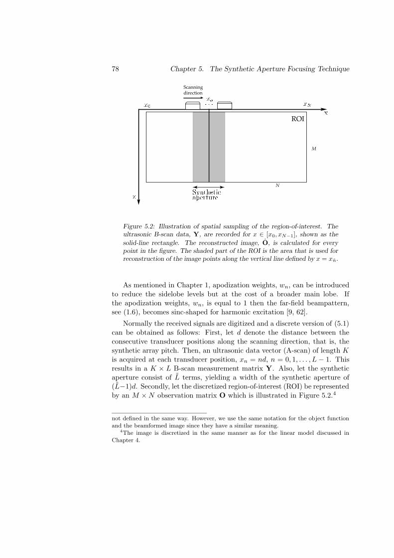
78 Chapter 5. The Synthetic Aperture Focusing Technique
ROI
Scanningdirection
M
N
Figure 5.2: Illustration of spatial sampling of the region-of-interest. Theultrasonic B-scan data, Y, are recorded for x ∈ [x0, xN−1], shown as the
solid-line rectangle. The reconstructed image, O, is calculated for everypoint in the figure. The shaded part of the ROI is the area that is used forreconstruction of the image points along the vertical line defined by x = xn.
As mentioned in Chapter 1, apodization weights, wn, can be introducedto reduce the sidelobe levels but at the cost of a broader main lobe. Ifthe apodization weights, wn, is equal to 1 then the far-field beampattern,see (1.6), becomes sinc-shaped for harmonic excitation [9, 62].
Normally the received signals are digitized and a discrete version of (5.1)can be obtained as follows: First, let d denote the distance between theconsecutive transducer positions along the scanning direction, that is, thesynthetic array pitch. Then, an ultrasonic data vector (A-scan) of length Kis acquired at each transducer position, xn = nd, n = 0, 1, . . . , L − 1. Thisresults in a K × L B-scan measurement matrix Y. Also, let the syntheticaperture consist of L terms, yielding a width of the synthetic aperture of(L−1)d. Secondly, let the discretized region-of-interest (ROI) be representedby an M × N observation matrix O which is illustrated in Figure 5.2.4
not defined in the same way. However, we use the same notation for the object functionand the beamformed image since they have a similar meaning.
4The image is discretized in the same manner as for the linear model discussed inChapter 4.

5.2. Performance of The Synthetic Aperture Focusing Technique 79
The discrete SAFT algorithm (5.1) can now be expressed as
(O)m,n =
n+L/2∑
n=n−L/2
wn(Y)k,n. (5.2)
The discrete time vector index, k, is a function of the distance between thetransducer position, xn, and the observation point, (xn, zm), that is givenby
k.=
(2
cp
√
(xn − xn)2 + z2m
)1
Ts. (5.3)
Note that since the signal is discrete, the time-shifts in (5.1) must be roundedtowards the nearest sampling instance which introduces some errors. Theoperator
.= denotes that k is rounded toward the nearest integer.5
5.2 Performance of The Synthetic Aperture Fo-
cusing Technique
Here a brief analysis of the SAFT performance is given. Since one of themain topics in this thesis is compensation of beampattern and diffractioneffects, we will treat these aspects for the SAFT algorithm below.
In SAFT experiments, the scanning transducer is normally small for thepurpose of creating an almost spherical beampattern. However, in manysituations a finite sized transducer must be used to obtain sufficient acousticpower. The diffraction effects due to a finite aperture will then reduceperformance, especially in the near-field. Undersampling may also causeproblems with grating lobes, in particular for narrowband systems. Someimportant parameters for the SAFT performance are:
• The bandwidth of the transducer.
• The size of the transducer’s active area.
• The synthetic array pitch.
• The F -number.
• The signal-to-noise ratio (SNR).
5It is common to perform interpolation or to oversample in order to reduce the roundingerrors.

80 Chapter 5. The Synthetic Aperture Focusing Technique
Below, the first four of these topics are discussed. The last one is post-poned to Chapter 8.
5.2.1 Spatial Undersampled Broadband Data
As mentioned in Chapter 1, the results from conventional far-field beam-pattern analysis of an undersampled array predict aliased lobes with thesame amplitude as the main lobe. However, for broadband imaging, spatialaliasing will in general be less severe, as shall be shown below.
Recall from Chapter 1 that, for a harmonic excitation signal and anarray pitch, d, that is larger than half the wavelength, λ/2, there will bestrong grating lobes in the angle interval -90 to 90 degrees outside the mainlobe. The grating lobes may severely deteriorate the processed image, sinceenergy from a target within the grating lobe will leak into the main loberesulting in spurious responses. The far-field beampattern,
|H(x, z)| =
∣∣∣∣∣∣
sin(
Ldπxλz
)
sin(dπx
λz
)
∣∣∣∣∣∣
, (5.4)
has a maximum at x = 0 but also for those points where the phase shifts ofthe received harmonic signals is a multiple of the wavelength at all transducerpositions. That is, all received signals arrive in phase for those points. Ifd < λ/2 then this will not occur.
Two example beampatterns computed using (5.4), for a point target atdepth z = 50 mm, is shown in Figure 5.3. The synthetic array pitch, d, was1 mm, and λ = 0.5 mm. Due to the undersampling grating lobes can befound around ±14 and ±28 mm for both apertures.
The beampattern in Figure 5.3 is valid also for tone-burst excitationprovided that the pulse length is sufficiently long. That is, if the sinusoidalsignal is too short, then all transducer positions will not contribute to thetotal output. If this is the case, then the amplitude in the grating lobewill drop and the effects of undersampling in SAFT is therefore less severecompared to harmonic excitation [9, p. 265].
Normally, in NDE and many other applications, broadband pulses areused and effects of undersampling will then depend of the pulse shape andlength [35, 72]. This effect is shown in Figure 5.5 where three differentsynthetic pulses, shown in Figure 5.4, have been used. The three pulseshad a half-power bandwidth (HPBW) of 89%, 28%, and 12%, respectively.

5.2. Performance of The Synthetic Aperture Focusing Technique 81
−30 −20 −10 0 10 20 30−40
−35
−30
−25
−20
−15
−10
−5
0
5
x [mm]
Nom
aliz
ed A
mpl
itude
[dB
]
d = 2λd = λ/2
(a) Beampattern for a synthetic aperture of 8 mm. d = 2λ(dash-dotted) and d = λ/2 (solid).
−30 −20 −10 0 10 20 30−40
−35
−30
−25
−20
−15
−10
−5
0
5
x [mm]
Nom
aliz
ed A
mpl
itude
[dB
]
−1.5 −1 −0.5 0 0.5 1 1.5−40
−30
−20
−10
0
x [mm]
(b) Beampattern for a synthetic aperture 50 mm (d = 2λ).
Figure 5.3: Beampattern for two synthetic apertures (8 and 50 mm) withan array pitch, d = 1 mm, for a target at z = 50 mm, and the wave-length, λ, was 0.5 mm. The inserted figure in (b) is an amplification of thebeampattern around x = 0.

82 Chapter 5. The Synthetic Aperture Focusing Technique
The bandwidth of 89% can be considered as high and 12% as relatively low.The sound field was simulated using the DREAM method for a circulartransducer and the simulation parameters are presented in Table 5.1.
Aperture [mm] 50
Depth z [mm] 50
Transducer diameter [mm] 0.4
Sound speed cp [m/s] 1500
Table 5.1: Parameters for the simulation results shown in Figure 5.5.
It is clear that the amplitudes of the grating lobes have been decreasedcompared to the narrowband analysis for all three pulses. Using a pulse witha HPBW of 89% resulted, for example, in a grating lobe level below -30 dB.The explanation for this behavior is simply that if the pulse is shorter thanLd sin(θ), where θ is the grating lobe angle, the pulse will not be present“simultaneously” at all transducer positions in the synthetic aperture andthe grating lobe amplitude will therefore drop. However, the pulse lengthcannot become arbitrarily short since the bandwidth of the array system islimited. Grating lobes will therefore always be a problem in undersampledDAS based array imaging.6
Note also that even though a shorter pulse alleviates the problem withgrating lobes, the lateral resolution does not improve significantly by using ashort pulse, cf. Figures 5.3(b) and 5.5. The lateral resolution depends mostlyon the synthetic aperture and the transducer size as will be discussed in thenext subsection.
5.2.2 Finite Sized Transducers and Lateral Resolution
As mentioned earlier in this chapter the transducer is assumed to be a pointsource and receiver in the SAFT algorithm. The validity of this assumptiondepends on the size of the transducer in relation to the distance to the focalpoint as well as the transducer’s center frequency and bandwidth.
As an example of typical SAFT performance for finite-sized transducers,
6It can also be seen in Figure 5.4 that the grating lobe pattern is smoother thanthe narrowband pattern, shown in Figure 5.3, since the amplitudes of many frequenciessuperimpose and since the grating lobes occur at different angles for different frequencies.

5.2. Performance of The Synthetic Aperture Focusing Technique 83
0 1 2 3 4 5 6 7
−1
−0.5
0
0.5
1
t [mus]
HPBW = 12.5 %
0 1 2 3 4 5 6 7
−1
−0.5
0
0.5
1
t [mus]
HPBW = 27.9 %
0 1 2 3 4 5 6 7
−1
−0.5
0
0.5
1
t [mus]
HPBW = 89.3 %
(a) Synthetic impulse responses.
0
0.2
0.4
0.6
0.8
1
0 2 4 6 8 10
f [MHz]
HPBW = 12.5 %HPBW = 27.9 %HPBW = 89.2 %
(b) Amplitude spectra.
Figure 5.4: Synthetic impulse responses and their corresponding amplitudespectra. The half-power bandwidths of the pulses are 12%, 28%, and 89%,respectively.

84 Chapter 5. The Synthetic Aperture Focusing Technique
−30 −20 −10 0 10 20 30−40
−35
−30
−25
−20
−15
−10
−5
0
5
x [mm]
Nom
aliz
ed A
mpl
itude
[dB
]
HPBW = 12.5 %HPBW = 27.9 %HPBW = 89.4 %
−1.5 −1 −0.5 0 0.5 1 1.5−40
−30
−20
−10
0
x [mm]
Figure 5.5: Beampattern profiles of broadband SAFT processed data withan aperture of 50 mm for the three pulses shown in Figure 5.4. The thin linecorresponds to a half-power bandwidth (HPBW) of 89%, the dash-dottedline to a HPBW of 28%, and the thick lines to HPBW of 12%. The insertedfigure is an amplification of the beam profiles around x = 0.
a simulation using the DREAM method for a short pulse7 and syntheticaperture of 50 mm, for a target at z = 50 mm, was performed. The beamprofile and 3 dB lobe width of the SAFT processed data are shown in Fig-ure 5.6 for a transducer radius ranging from 0.005 to 5 mm. The 0.005mm transducer can be considered as very small and the 5 mm transduceras large. That is, the 5 mm transducer is large enough to manifest strongbeam directivity effects.
As can be seen in Figure 5.6, the resolution clearly deteriorates as thesize of the transducer increases. There is nearly a linear relationship be-tween beam width and transducer size, cf. Figure 5.6(b). Note that in thisexample, if the transducer is larger than approximately 3.5 mm the lateralresolution becomes even worse than the unprocessed data.
To further illustrate the behavior of the SAFT algorithm, B-scan im-ages of unprocessed and SAFT processed simulated data is shown in Fig-ure 5.7. Results from two transducer sizes are shown where the first one is
7The pulse with the half power bandwidth (HPBW) of 89% shown in Figure 5.4 wasused.

5.3. Matrix Formulation of the SAFT Algorithm 85
−5 −4 −3 −2 −1 0 1 2 3 4 50
0.1
0.2
0.3
0.4
0.5
0.6
0.7
0.8
0.9
1
x [mm]
Nor
mal
ized
Am
plitu
de
r=0.005 mmr=0.5 mmr=2 mmr=5 mm
(a) Broadband beam profile for 4 differ-ent transducer sizes.
0 1 2 3 4 50
1
2
3
4
5
6
7
8
9
10
Transducer radius [mm]
3 dB
wid
th [m
m]
SAFTUnprocssed
(b) 3 dB beam width as function oftransducer size for unprocessed- andSAFT-processed data.
Figure 5.6: Lateral resolution for SAFT processed data for transducer sizesfrom 0.005 to 5 mm. The simulations were performed with an aperture of50 mm for a target at z = 50 mm.
small (0.005 mm) and the second large enough to manifest strong transducersize effects. The unprocessed data for the small transducer, shown in Fig-ure 5.7(a), shows the typical hyperbolic form resulting from linear scanningwhen the transducer emits nearly spherical waves. It is this pattern thatthe hyperbola in the SAFT algorithm (5.1) is matched against. The datafrom the large transducer (5 mm) shown in Figure 5.7(b) deviates, however,significantly from the hyperbolic form. The SAFT performance is thereforepoor for the large transducer whilst the result from the small transducershows a significant improvement in lateral resolution compared to the un-processed data, cf. Figures 5.7(d) and 5.7(c). Consequently, the diffractioneffects of the transducer can severely deteriorate the lateral resolution if careis not taken.
5.3 Matrix Formulation of the SAFT Algorithm
The time-domain SAFT algorithm can also be expressed using a matrixformalism. Here this is done in the interest of clarity. Furthermore, thematrix formulation of SAFT enables a direct comparison with the later

86 Chapter 5. The Synthetic Aperture Focusing Technique
x [mm]
t [µ
s]
−10 −5 0 5 10
65.5
66
66.5
67
67.5
68
(a) Unprocessed B-scan for the 0.005mm transducer.
x [mm]
t [µ
s]
−10 −5 0 5 10
65.5
66
66.5
67
67.5
68
(b) Unprocessed B-scan for the 5 mmtransducer.
x [mm]
z [m
m]
−10 −5 0 5 10
49
49.2
49.4
49.6
49.8
50
50.2
50.4
50.6
50.8
51
(c) SAFT processed image for the0.005 mm transducer.
x [mm]
z [m
m]
−10 −5 0 5 10
49
49.2
49.4
49.6
49.8
50
50.2
50.4
50.6
50.8
51
(d) SAFT processed image for the 5mm transducer.
Figure 5.7: B-mode images of unprocessed and SAFT processed simulateddata for two transducer sizes. The simulations were performed with anaperture of 50 mm for a target at z = 50 mm using a wide band pulseexcitation with a HPBW of 89%.

5.3. Matrix Formulation of the SAFT Algorithm 87
proposed algorithms for better illustration of the relations between them.
Let O denote the SAFT reconstructed image. The reconstructed imagetakes the values at the spatial sampling points xn, zm) for n = 0, . . . , L − 1and m = 0, . . . , M − 1, respectively.
Again, let yn = [uo(xn, t0) uo(xn, t1) · · ·uo(xn, tK−1)]T denote the nth
A-scan column vector in Y. The DAS operation can now be expressed as asummation of matrix-vector multiplications, that is, the nth column, on, inO can be expressed as
on =
n+L/2∑
n=n−L/2
Dd(n,n)yn (5.5)
where d(n, n) is defined in (4.18) and Dd(n,n) is given by
(Dd(n,n))m,j =
{
wd(n,n) for j = k (with k defined in (5.3)),
0 otherwise.(5.6)
The apodization weight wd(n,n) can be a rectangular window function, i.e.,wd(n,n) is identical to 1, but often it is a decreasing function of the distanced(n, n).
By following the notation introduced in Chapter 4, where the data vectorwas defined as y = vec(Y) , [yT
0 yT1 · · ·yT
L−1]T , and the vectorized image as
o = vec(O), and by also noting that d(n, n) = d(n + i, n + i) for any integeri, the SAFT algorithm can finally be expressed as
o =
Dd(i−L/2,i)... Dd(i−L/2,i) 0
Dd(i+L/2,i)
...
Dd(i+L/2,i)
. . .
. . . Dd(i−L/2,i)
0...
Dd(i+L/2,i)
y0
y1
...
yL−1
=DTsafty,
(5.7)

88 Chapter 5. The Synthetic Aperture Focusing Technique
for any i such that i−L/2 and i+L/2 is in the ROI. Note also that k in (5.6)is a function of (xn − xn)2, implying the symmetry relation Dd(n−n,n) =Dd(n+n,n). The matrix Dsaft is a KL × MN sparse block matrix.
5.4 Matched Filter Interpretation
The SAFT algorithm can be viewed as an implementation of a matched filter(MF) [6, 9], where the filter associated with image point (xn, zm) is givenby the hyperbolic function (5.3). The matched filter is the linear filter thatmaximizes the SNR for a known signal with known arrival time [73, 74].Consider the one-dimensional discrete time case with a signal s in Gaussiannoise,
y = s + e. (5.8)
The filter, h, that maximizes the SNR is given by [73]
h ∝ C−1e s, (5.9)
where Ce is the noise covariance matrix. If the noise is white (Ce = σ2eI) the
MF output, hTy = sTy, is simply a correlation with the signal prototypes. In the SAFT case, the hyperbola, defined in (5.3), is the 2D MF forthe response from a single point target at image point (xn, zm), given thatthe transducer can be well approximated as a point source and that theits forward and backward electro-mechanical impulse responses, hef(t) andheb(t), are delta functions, cf. Figure 4.1. Under these circumstances theSNR is expected to increase after SAFT processing
Each column in the SAFT matrix, Dsaft, defined in (5.7) contains thematched filter for the corresponding image point. That is, by using (5.7)the SAFT matched filter outputs are computed simultaneously for all imagepoints.
Using the linear model derived in Chapter 4 the image obtained afterSAFT processing can be modeled as
o =DTsafty
=DTsaft(Po + e),
(5.10)
where, y = Po + e, was introduced in (4.23). The columns in the matrixDT
saft acts as a masks that “picks out” the samples in y corresponding tothe hyperbolas given by (5.3).

5.5. Remarks 89
5.5 Remarks
Note that for the SAFT algorithm to be a true matched filter, DTsaft must
equal PT otherwise will the SAFT filters not match the true response ex-actly. Recall from Chapter 4 that the ith column, pi, in the propagationmatrix P corresponds to the response from a unit area point target at theimage point represented by the ith element in the vectorized image o. TheMF for that image point is then pT
i y This transpose operation can be seenas a time-reversal of the propagation operator that maximizes the amplitudeof the acoustic wave at a given time and location [75].
In the far-field, and for very broadband systems, the approximationDT
saft ≈ PT may be reasonable but in the near-field there are a numberof issues that only make the SAFT algorithm an approximation of a MF:
• The electrical impulse response of the transducer filters the signal sothat even if the input signal is a delta function the temporal waveformwill not resemble a delta function. Since SAFT uses delta functions(time-delays) temporally the SAFT MF will not match the true wave-form.
• SAFT treats the transducer as a point source and receiver. If thetransducer has a finite size the SIRs associated with the transducerwill smoothen waveform which also leads to a mismatch between theSAFT filters and the true response.
It should also be emphasized that MFs is only optimal in the sense thatthey maximize the SNR at one point when one signal is present. A MFprocessing will therefore not necessarily result in high resolution images sinceenergy from scatterers nearby to the observation point may leak into thefocal point, through the side- or grating lobes associated with the MF [44].

90 Chapter 5. The Synthetic Aperture Focusing Technique

CHAPTER 6
Real Aperture Array Imaging
REAL aperture array imaging plays an important role in ultrasonic imag-ing.1 The reason for the popularity is the very high flexibility of this
technique. Real arrays makes it possible to design very fast electronic beamscanning systems as well as fast switching of the focusing properties of thebeam.
In this chapter we will review some important properties of real aperturearray imaging. We focus on two topics, the transmit process of a phasedarray,2 and parallel receive beamforming. The purpose of this chapter ismainly to familiarize the reader with some characteristics of broadband realaperture array imaging that we later will come back to in the followingchapters in this thesis.
Note that, we will only consider classical delay-line type of systems thatfocus the beam by means of imposing time delays on the signals driving thearray elements. That is, we will not consider the type of systems that havestarted to appear in the last decade that are capable of exciting the arrayelements with arbitrary waveforms [76, 77].
This chapter is organized as follows: In Section 6.1, classical CW far-fieldarray modeling is discussed. In particular, beam steering and its influence
1By real aperture array imaging we mean imaging with physical arrays.2The receive process is not discussed here since it is very similar to the receive process
in synthetic aperture imaging discussed in Chapter 5. The main difference between a realand a synthetic aperture is that a real aperture allows for simultaneous acquisition fromall array elements while using a synthetic aperture one acquire the data sequentially.
91

92 Chapter 6. Real Aperture Array Imaging
on grating lobes are mentioned. In Section 6.2, some important propertiesof broadband array imaging are treated, in particular, the influence of thearray element size and the interrogated wave form is discussed. Finallyin Section 6.2, parallel array imaging is briefly introduced and a matrixexpression for a parallel DAS beamformer is presented.
6.1 Conventional Narrowband Transmit Beamform-
ing Analysis
In Chapter 1, conventional delay-and-sum (DAS) beamforming was intro-duced. In particular, the effects of apodization as well as spatial samplingconsequences, such as grating- and sidelobes are discussed. We will, there-fore, assume that the reader is already familiar with these concepts. In thissection we will extend the analysis to transmit beamforming, still treatingthe array elements as point sources and assuming CW excitation. Theseassumptions will then be relaxed in the next section where broadband arrayimaging, with finite sized elements, are discussed. This is done here in or-der to show the differences between the common CW far-field beam patternanalysis, where idealized arrays with point-like elements are assumed, anda broadband excitation with more realistic array models.
Consider a 1D phased array consisting of L elements equally spaced alongthe x-axis with an array pitch d, see Figure 1.8 in Chapter 1. The positionvector, rn, for the nth element is then rn = (xn, 0, 0). Since the waveswill spread spherically from the point-like elements, the wave field at anobservation point, r, will become a sum of the spherical wave contributionsfrom each element. If we also apply the paraxial approximation introducedin Section 1.2 for the amplitude terms of the waves, then the CW field at r
can be approximated by
H(r, t) ≈L−1∑
n=0
wnejω(t−
|r−rn|cp
+τn), (6.1)
where wn is the apodization weight for the nth element and τn is the cor-responding focusing delay. Focusing at a point rf can now achieved byassigning the time delay, τn = |rf−rn|
cp, for n = 0, 1, . . . , L−1. If rf is located
on the z-axis then the array is focused but not steered, otherwise the arrayis also steered.
To show the effect of focusing and beam steering, consider a 16 elementphased array with a pitch d = 2λ and focused at z=50 mm (cp = 1500

6.2. Broadband Transmit Beamforming with Finite Sized Array Elements93
m/s, λ = 0.5 mm). This is an undersampled array and grating lobes willtherefore appear. Two example CW fields for the array are in shown Fig-ure 6.1. Figure 6.1(a) shows the wave field when the array is focused butnot steered and the corresponding beam pattern, at z = 50 mm, is shownin Figure 6.1(c). Similarily, the wave field for the array steered -20 degrees,is shown in Figure 6.1(b) and the corresponding beam pattern is shown inFigure 6.1(d).
Clearly, the undersampling manifests itself in several grating lobes bothfor the non-steered and the steered array. Also, as can be seen in Fig-ure 6.1(b) and (d), beam steering not only steers the main lobe but alsothe grating lobes. Measurements often are performed in such way that it ismore likely for a scatterer to be located close to the center of the array andthe problem with ghost responses due to grating lobes are, therefore, moresevere for steered systems than for non-steered systems.
Note, however, that the model (6.1) neither considers the beam directiv-ity of the elements nor the fact that the length of a the transmit pulse—ifa broadband pulse is used—also influences the grating- and sidelobe ampli-tudes. These topics are further discussed in the next section.
6.2 Broadband Transmit Beamforming with Fi-
nite Sized Array Elements
In Chapter 5 it was shown that the transducer size had a large impact on thelateral resolution for SAFT processed data. In this section we will discusssome of the effects that the transducer size, or more specifically, the arrayelement size has on the transmitted wave field for broadband excitation ofa real aperture array.
In the narrow band analysis in the previous section we saw that bysteering the beam also the grating lobes was steered. Due to the paraxialapproximation, the max amplitude in the main beam and in the gratinglobes were the same, cf. Figure 6.1(b). For a more realistic array, with finitesized array elements, this will in general not be the case [78]. To see this,let us study an example.
Consider again a phased array with the same pitch and aperture aswas used in the CW example in the previous section, that is, a 16 elementarray with a pitch of 1 mm focused at z =50 mm. But now the elementshave a finite size; they are circular with a diameter of 0.9 mm. Also, a
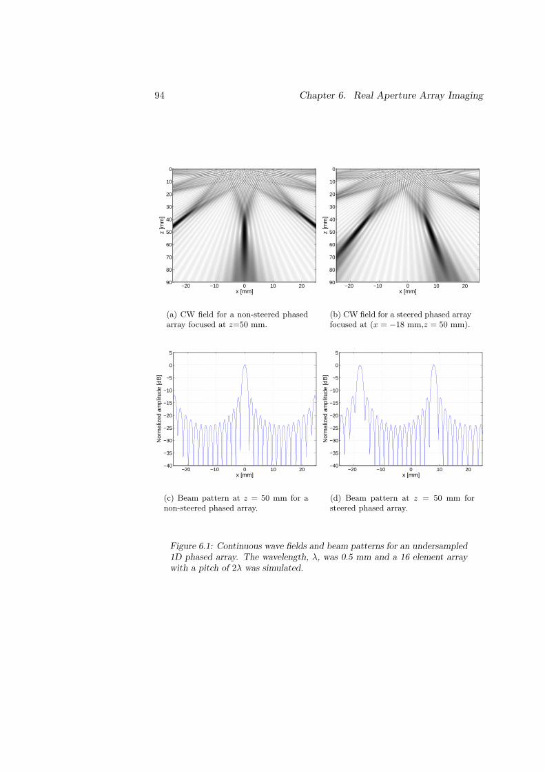
94 Chapter 6. Real Aperture Array Imaging
z [m
m]
x [mm]−20 −10 0 10 20
0
10
20
30
40
50
60
70
80
90
(a) CW field for a non-steered phasedarray focused at z=50 mm.
z [m
m]
x [mm]−20 −10 0 10 20
0
10
20
30
40
50
60
70
80
90
(b) CW field for a steered phased arrayfocused at (x = −18 mm,z = 50 mm).
−20 −10 0 10 20−40
−35
−30
−25
−20
−15
−10
−5
0
5
x [mm]
Nor
mal
ized
am
plitu
de [d
B]
(c) Beam pattern at z = 50 mm for anon-steered phased array.
−20 −10 0 10 20−40
−35
−30
−25
−20
−15
−10
−5
0
5
x [mm]
Nor
mal
ized
am
plitu
de [d
B]
(d) Beam pattern at z = 50 mm forsteered phased array.
Figure 6.1: Continuous wave fields and beam patterns for an undersampled1D phased array. The wavelength, λ, was 0.5 mm and a 16 element arraywith a pitch of 2λ was simulated.

6.2. Broadband Transmit Beamforming with Finite Sized Array Elements95
broadband pulse is used, which is shown in Figure 3.4(a) in Chapter 3. Thepulse has a center frequency of approximately 3 MHz which corresponds toa wavelength, λ, of 0.5 mm. Thus, the array is undersampled and gratinglobes should appear.
Simulated wave field snapshots, at three time instants, for this arraysetup are presented in Figure 6.2. The snapshots where computed usingthe DREAM method, for the array focused at z = 50 mm, both for anun-steered and a steered configuration.3
By comparing the CW interference patterns, shown in Figure 6.1(a) and(b), with the broadband fields, shown in Figure 6.2(a) and (b), one canobserve that the somewhat chaotic interference patterns close to the arrayseen in the CW images cannot be observed in the broadband snapshots.Instead, the waves are almost planar shortly after they have left the arrayfor the broadband case.
As time evolves, and the waves approaches the focal points, the wavefields become more concentrated. When they have reached z = 50, shownin Figure 6.2(e) and (f), the waves fields are rather narrow.
However, due to the undersampling of the array aperture, one can alsoobserve significant acoustic energy outside the main beams, see Figure 6.2(c)–(f). This is more easily seen in the profile plots of the wave fields shown inFigure 6.3. These profile plots were taken when the waves had reached thefocal points. By comparing the profile plots, shown in Figure 6.3, with theCW beampatterns, shown in Figure 6.1(c) and (d), one can notice that theamplitudes of the grating lobes, with respect to the main lobes, are signifi-cantly lower in the broadband profile plots. The reason for this behavior istwofold:
• The length of the pulse is only about two cycles (of the center fre-quency), cf. Figure 3.4(a). Hence, only the signal from two elementswill add constructively at the grating lobe, in contrary to CW excita-tion, where the signals from all elements adds in phase at the gratinglobes [9].
• The beam directivity of the elements results in significantly reducedamplitudes at observation points far from corresponding array element.
The beam directivity of the elements will, therefore, influence the beamsteering properties of the array; the element’s beam directivity essentially
3The array was steered -20 degrees.

96 Chapter 6. Real Aperture Array Imaging
x [mm]
z [m
m]
−20 −10 0 10 20
0
10
20
30
40
50
60
70
80
(a) Snapshot at t = 10µsa for a non-steered phasedarray.
x [mm]
z [m
m]
−20 −10 0 10 20
0
10
20
30
40
50
60
70
80
(b) Snapshot at t = 10µsfor a steered phased array.
x [mm]
z [m
m]
−20 −10 0 10 20
0
10
20
30
40
50
60
70
80
(c) Snapshot at t = 22µsfor a non-steered phasedarray.
x [mm]
z [m
m]
−20 −10 0 10 20
0
10
20
30
40
50
60
70
80
(d) Steered Array. Snap-shot at t = 22µs.
x [mm]
z [m
m]
−20 −10 0 10 20
0
10
20
30
40
50
60
70
80
(e) Snapshot at t = 37.6µsfor a non-steered phasedarray (where the wave isclose to the focal point).
x [mm]
z [m
m]
−20 −10 0 10 20
0
10
20
30
40
50
60
70
80
(f) Snapshot at t = 37.6µsfor a steered array (wherethe wave is close to the fo-cal point).
Figure 6.2: Broadband field snapshots for an undersampled phased arraywith circular array elements. The center frequency of the broadband pulsecorresponds approximately to a wavelength, λ, of 0.5 mm and a 16 elementarray with a pitch of 2λ was simulated.

6.2. Broadband Transmit Beamforming with Finite Sized Array Elements97
−20 −10 0 10 20−40
−35
−30
−25
−20
−15
−10
−5
0
5
x [mm]
No
rma
lize
d a
mp
litu
de
[d
B]
(a) Non-steered Array. Profile at t =37.6µs
−20 −10 0 10 20−40
−35
−30
−25
−20
−15
−10
−5
0
5
x [mm]
No
rma
lize
d a
mp
litu
de
[d
B]
(b) Steered Array. Profile at t = 37.6µs
Figure 6.3: Broadband profiles for the wave fields shown in Figure 6.2(e)and (f) respectively.
reduces the effective aperture of the array. To illustrate this, consider theprofile plot of the wave field for one element, at x = 7.5 mm, shown inFigure 6.4. The profile plot was taken at t = 34.1µs and the pulse hasthen traveled approximately 50 mm in the medium. As can be observed,the amplitude at x = −10 mm is about 20 dB lower than directly underthe array element, at x = 7.5. Thus, if the steering angle is high then thecontributions from elements at a horizontal distance far from the focal pointwill become very low.
From the discussion above it is clear that many factors must be taken intoaccount when choosing a proper array layout for broadband ultrasonic arrayimaging. The simplified far-field CW model (6.1) is often not sufficient sincemany important properties are not considered by that model. To successfullyanalyze broadband array imaging one must in particular consider the sizeeffects of the array elements as well as the waveform of interrogated pulse.
We will come back to these topics in Chapters 7 and 8 when we discussreconstruction methods for ultrasonic array imaging.

98 Chapter 6. Real Aperture Array Imaging
−20 −10 0 10 20−40
−35
−30
−25
−20
−15
−10
−5
0
5
x [mm]
No
rma
lize
d a
mp
litu
de
[d
B]
Figure 6.4: Broadband beam profile for a single circular array element witha diameter of 0.9 mm at t = 34.1µs. The vertical line indicates the positionof the array element.
6.3 Parallel Receive Beamforming
Parallel beamforming is a method developed to increase the frame rate ofarray imaging systems. The basic idea is the transmit a broader-than-normalbeam and then beamform several image lines from that transmission. Thiswill decrease the number of re-transmissions needed to cover the whole ROI,thus increasing the image frame rate [79, 80].
In this section we will consider parallel DAS beamforming whilst moreadvanced approaches will be discussed in Chapter 8.
A parallel receive mode DAS beamformer consists of several delay-lineunits, thus enabling focusing at many points. A schematic block diagramof a parallel DAS beamformer is shown in Figure 6.5. Similar to the SAFTalgorithm, the parallel DAS beamformer can be expressed using matrix for-malism as shown below.
Let us for simplicity consider 2D parallel beamforming where the ROIhas been discretized and represented by an M × N matrix O as describedin Chapter 4.
Consider again a 1D array with L elements positioned along the x-axis.Let yn denote the A-scan received by the nth array element, yn = [uo(xn, t0)uo(xn, t1) · · ·uo(xn, tK−1)]
T , and y, the (vectorized) B-scan containing theA-scan data for all elements, y , [yT
0 yT1 · · ·yT
L−1]T . Then, the operation of

6.3. Parallel Receive Beamforming 99
n
n
n
~
~
~
Figure 6.5: Block scheme of a parallel delay-and-sum beamfomer. Eachdelay-line unit is focused at a different observation point.
one of the delay-line units, focused at the observation point (xn, zm), can beexpressed as
(O)m,n =L−1∑
n=0
wnuo(xn, τn(xn, zm))
=L−1∑
n=0
wnyTnd(m,n)
n
=
w0d(m,n)0
w1d(m,n)1...
wL−1d(m,n)L−1
T
y,
(6.2)
where wn is an apodization weight, τn(xn, zm) is the focusing delay for fo-

100 Chapter 6. Real Aperture Array Imaging
cusing at the observation point (xn, zm), and d(m,n)n is a vector of length K
which is zero everywhere except at the kth index, k.= τl(xn,zm)
Ts, where it is
1.
Now, the total vectorized image, o = vec(O), for all observation points,
can be expressed by appending the delay vectors, d(m,n)n , for the remaining
observation points, according to
o =
w0d(0,0)0 w0d
(1,0)0 · · · w0d
(M−1,N−1)0
w1d(0,0)1 w1d
(1,0)1 · · · w1d
(M−1,N−1)1
......
...
wL−1d(0,0)L−1 wL−1d
(1,0)L−1 · · · w1d
(M−1,N−1)L−1
T
y
= Kdasy.
(6.3)
The operation described by (6.3) is similar to that of a dynamic focus
beamformer. A dynamic focusing beamformer has time-dependent focusdelays which, in receive mode, adapts focusing at the same rate as the wavepropagates. This results in an extended region where the beam is focusedcompared to a fixed focus beamformer. The matrix Kdas in (6.3) acts asa dynamic focus beamformer that focuses, in parallel, at all observationpoints.

Part III
Bayesian Ultrasonic Image
Reconstruction
101


CHAPTER 7
Ultrasonic Image Reconstruction Methods
RECALL from Chapter 1, that the main objective in all ultrasonic imag-ing applications is that we want to gain knowledge of an object under
study by means of studying the ultrasonic scattering from the object. Weperform experiments and by observing the recorded data we draw conclu-sions whether, for example, a defect is critical or not or, in a medical appli-cation, whether surgery must be performed or not. The data can however bedifficult to interpret for a human operator since the wave propagation in themedium can be complex and the measurement apparatus may distort thereceived scattering information. That is, the user must have deep knowledgeabout the measurement system in order to draw accurate conclusions fromthe experiment.
The focusing methods discussed in Chapters 5 and 6 can alleviate thisprocess to some degree. Focusing, or beamforming, is performed mainly fortwo reasons:
• The obtained ultrasonic images are easier to interpret when the acous-tic energy is concentrated to a small region.
• The acoustic energy, in the region that we want to study, must be highenough to obtain a sufficient SNR since, otherwise, the data will notcontain enough information regarding the scattering objects.
It should however be noted that receive mode beamforming does not giveus any additional information than what is already in the unprocessed data
103

104 Chapter 7. Ultrasonic Image Reconstruction Methods
received from the individual array elements, rather the opposite. This factis known as the data processing inequality which states that: no processingof the data, deterministic or random, can increase the information that thedata contains of the parameter we want to estimate [81]. In practice, allprocessing that we perform on the data will in fact destroy some amount ofinformation due limited numerical precision, etc.
A relevant question that we can ask us is: How should we process our data
to utilize its information about the scattering strengths in the best possible
way to obtain a result that can be easily understood by a human? In manyapplications DAS based methods may be sufficient for the particular purposebut they are not optimal in the sense of utilizing all available information.A reasonable answer to the question formulated above is that we should useall information that is available, both from data and from prior knowledge.We know, for example, many properties of the measurement system andthe linear model described in Chapter 4 gives us a tool for modeling thesystem’s “distortion”. This knowledge can then be used to compensatefor the distortion and thereby obtaining images that should be easier fora user to understand. In other words, if we formulate the problem as animage reconstruction problem we may be able to improve the image qualitycompared to traditional DAS beamforming.
The system model is however not the only prior information that wehave. We also know that the scattering amplitudes cannot become arbitrar-ily large since the ultrasonic transducer emits a finite amount of acousticenergy. In some cases we may even know the sign of the scattering ampli-tude. An optimal reconstruction method, that accounts for all information,should therefore use both the prior information and the information fromthe experiments.
We must bear in mind that we cannot expect to fully recover the truescattering image (with arbitrary precision) since we never have completeinformation. The data are acquired using a limited aperture, often froma a 1D array, and we cannot expect to reconstruct a 3D object based on2D data. Furthermore, the data are always corrupted by thermal noise andthe models we use do always have limitations. It is evident that there willalways be an amount of uncertainty in our estimates. This lack of completeinformation usually manifest itself in making the problem ill-posed. Thatis, if we deductively try to find an inverse to the propagation operator, thenthis inverse will not be stable in the sense that a small disturbance can causea large change in the estimates. When solving inverse problems deductivelyone must therefore take special measures to stabilize the solution. This

105
process is usually called regularization and a popular method is the so-called Tikhonov regularization [31]. Regularization typically involves tuningparameters to compromise between fidelity to the data and the stability ofthe solution.
Another approach is to view the problem as a Bayesian inference prob-lem. In the Bayesian philosophy the prior information has a central roleand, for inference problems, the regularization parameters can be directlyconnected to the prior knowledge. In fact under certain conditions, theTikhonov regularization schemes can be seen as a special case of the linearminimum mean squared estimator derived using Bayesian analysis, althoughTikhonov regularization is based on totally different assumptions.
As mentioned in Chapter 1, ultrasonic imaging experiments easily pro-duce large data volumes and the dimensionality of the problems are oftenvery high. Practically, there is a trade off between computational complex-ity and the quality of the results. The reconstruction methods proposed inthis chapter, have been developed with that in mind. The problem has beenformulated from a Bayesian perspective where regularization parameters canbe deduced from the prior information of the scattering strength, typicallythe scattering mean value or the variance, and the variance of the noise.
In this chapter two Bayesian estimators are derived, one linear and onenon-linear. The linear estimator is based on the assumption that the meanand variance of the scattering strengths are known. This results in thelinear minimum mean-squared error (MMSE) estimator. The non-linearestimator is based on the assumptions that we are imaging objects withpositive scattering strengths that we know the mean of. It is shown thatthe resulting maximum a posteriori (MAP) solution is found by solvinga quadratic programming (QP) problem. Also found in this chapter is acomparison of the two Bayesian methods with common methods for solvingill-posed inverse problems.
The chapter is organized as follows: In Section 7.1, a short introductionto Bayesian inference is presented and the maximum entropy principle, usedfor assigning prior probability density functions, is introduced. This sectionalso includes derivations of the optimal linear MMSE estimator, as well asthe optimal non-linear exponential MAP estimator. In section, 7.2, somecommon methods for solving ill-conditioned image reconstruction problemsare reviewed and the relation to the Bayesian estimators are discussed. Inparticular it is shown that, under certain conditions, these methods canbe seen as a special case of the linear Bayesian estimator discussed in Sec-

106 Chapter 7. Ultrasonic Image Reconstruction Methods
tion 7.1. This section also contains a discussion of the maximum likelihoodestimator and its properties. Finally, in Section 7.3, some concluding re-marks are given.
7.1 Bayesian Image Reconstruction
In Bayesian estimation theory a probability density function (PDF) de-scribes the uncertainty, or the degree of belief, of the true value of thevariable under study [82]. In other words, a PDF is thought of as a carrier
of information. In our case we want to study the scattering strength at eachimage point described by the vector o. To accomplish this we perform anexperiment that gives us some data y. Note, that our knowledge regarding o
is usually not only coming from the data. Typically we know, without seeingany data, that o cannot have an arbitrary scattering amplitude; the scatter-ing amplitude must at least be limited to some interval. The PDF, p(o|I),that describes our knowledge before seeing the data is usually called “theprior” and I denotes any background information that we have regarding o.When we have performed an experiment we have received more informationabout o and the updated PDF after seeing the data is given by the posterior
PDF, p(o|y, I). If the measurement contained relevant (new) informationof o then the posterior PDF should be more concentrated around the truevalue of o.1
Bayes’ theorem,
p(o|y, I) = p(o|I)p(y|o, I)
p(y|I), (7.1)
describes how to update our knowledge of the variable, o, when new data,y, is observed. The conditional PDF p(y|I) is a normalization factor notdependent on o and p(y|o, I) describes the likelihood of seeing the data y
given o.
In this thesis the measurement errors are assumed to be Gaussian andp(y|o, I) will therefore be given by the multidimensional Gaussian distribu-tion,
p(y|o, I) =1
(2π)MN
2 |Ce|1/2e−
12(y−Po)T Ce
−1(y−Po), (7.2)
1If the prior PDF and the posterior PDF are identical we know that the data containsno new information of the variable.
7.1. Bayesian Image Reconstruction 107
where P is the propagation matrix from (4.23) and the size of the image toreconstruct is M × N .
The two most common estimators in Bayesian estimation applicationsare the maximum a posteriori (MAP) estimator and the minimum meansquare error (MMSE) estimator. The MAP estimate is found by maximizingp(o|y, I) and take the maximizing argument as the estimate,
omap = arg maxo
p(o|y, I) = arg maxo
p(o|I)p(y|o, I), (7.3)
where (7.1) was used in the last equality. The MAP estimate is thus thevalue o that is most probable given both data and prior information.
The MMSE estimate is given by
ommse = arg mino
E{‖o − o‖2} (7.4)
where E{·} is the expectation operator. It should be emphasized that it isonly when both o and e are Gaussian that the MMSE estimate is practi-cally tractable. The reason is that when both o and e are Gaussian theMMSE estimate will be a linear combination of the data. If o and e are notGaussian, then Markov chain Monte-Carlo (MCMC) methods can be usedto draw samples from p(o|y, I) and then average over these samples [83].This is however very time consuming for high dimensional problems and istherefore not practical for the applications described in this thesis.
Furthermore, if both o and e are Gaussian then the MAP and the linearMMSE estimate will be identical. Although this is well known we presentthe respective solutions here for practical reasons. Consider first the lin-ear MMSE estimate, defined as the estimate o = Ky that minimizes thecriterion,
Jmse(K) = E{‖o − Ky‖2}. (7.5)
with y = Po + e. The linear MMSE estimator, Kmmse, is then given by
Kmmse = arg minK
E{‖o − Ky‖2}
= arg minK
E{(o − Ky)T (o − Ky)}
= arg minK
tr{Co} − 2 tr{KTCoPT } + tr{KPCoP
TKT }
+ tr{KCeKT }
(7.6)
where we assumed that o and e are mutually independent with covariancematrices Co = E{ooT } and Ce = E{eeT }, respectively. Taking the deriva-tive with respect to K and equating to zero in (7.6) results the linear MMSE

108 Chapter 7. Ultrasonic Image Reconstruction Methods
estimateommse = Kmmsey = CoP
T (PCoPT + Ce)
−1y (7.7)
The MAP estimate can be found by again assuming that o and e arezero mean Gaussian. Now take the negative logarithm of (7.1), excludingall terms not dependent on o, which results in the criterion
Jmap(o) =1
2oTCo
−1o +1
2(y − Po)TCe
−1(y − Po) (7.8)
Differentiating (7.8) with respect to o and equating to zero gives the MAPsolution
omap = (C−1o + PTC−1
e P)−1PTC−1e y = Kmapy. (7.9)
The equivalence of (7.9) and (7.7) is discussed in Appendix 7.A.1. Thisequivalence is of practical interest since the matrix inverse in (7.7) and theinverse (C−1
o + PTC−1e P)−1 in (7.9) may be of different size.2 Recall from
Chapter 4 that the A-scan dimension is K and the number of measurementsis L, resulting in a KL × KL noise covariance matrix Ce, and that thenumber of observation points is MN , resulting in an MN ×MN covariancematrix Co. Hence, if KL is larger than MN , then it is less computationallydemanding to use the MMSE form compared to the MAP form and viceversa.3
Another important feature of Bayesian methods is that we obtain a mea-sure of the precision of the estimate. For Gaussian o and e, the PDF for theerror, ε = ommse − o, for the linear MMSE estimate is also Gaussian withzero mean and the covariance matrix,
Cε = E{(ommse − o)(ommse − o)T } = E{εεT }, (7.10)
given by (see also Appendix 7.A.2) [84]
Cε = Co − CoPT (Ce + PCoP
T )−1PCo
= (C−1o + PTC−1
e P)−1.(7.11)
The mean squared error (MSE) is the sum of the diagonal elements of Cε
Jmse , tr{Cε}. (7.12)
2A matrix inverse requires a number of operations in the order of n3 where n is thedimension of the matrix.
3A typical A-scan dimension, for the experiments presented later in this thesis, isK = 1000, and L = 16 for the real aperture array experiments. If O, for example, is an100 × 50 image, then P has the dimension 16000 × 5000, which is a normal size of theproblems treated in this thesis.

7.1. Bayesian Image Reconstruction 109
If the noise energy is large, that is Ce � PCoPT , then Cε is approximately
equal to Co. We know then that our reconstruction performance is poorand we should choose to design the experiment differently. Moreover, sinceeach diagonal element in Cε corresponds to the variance at an observationpoint, the expected error due to a chosen focusing method can be evaluatedby organizing the diagonal elements into an M × N image. By observingthe expected mean-squared error image it can then be directly seen in whatregions the reconstruction performance is acceptable and where it is not.This topic will be further discussed in Chapter 9.
7.1.1 Assigning Prior Probability Density Functions — The
Maximum Entropy Principle
So far we have not discussed how to obtain the prior p(o|I). In the lin-ear MAP estimate (7.9) it was assumed that the prior was Gaussian. TheGaussian PDF is uniquely determined by the mean vector and the covari-ance matrix; hence it seems reasonable to assign a Gaussian prior if the onlyinformation about o we have is the mean and the variance. The question isif this assumption can be justified?
If we have no prior information of the scattering amplitudes, then allamplitudes are equally likely. This corresponds to a uniform distributionwith infinite support. Hence the uniform PDF is the most “uninformative”of all distributions; the uniform distribution represents the most noncom-mittal distribution since no amplitude is favored over any other. However,by using a uniform prior PDF with infinite support we have not used thatwe know the mean and variance which is undesirable. A reasonable require-ment is thus that the prior PDF should be maximum non-committal withrespect to the, in this case, known mean and variance. Hence, we want theprior be as uninformative as possible but take into account the informationthat we actually have.
To judge how uninformative a PDF is we need a consistent measure ofits “uniformity”. This measure can then me maximized with respect tothe constraints given by our prior information; thus yielding a prior that ishonest about what we know. The measure should be continuous, consistent,and a monotonic increasing function in the sense that if n events are equallylikely, then the measure should increase if n increases. That is, we are moreuncertain which event that will occur if there are many possibilities thanwhen there are few. The only known function with these properties is the
110 Chapter 7. Ultrasonic Image Reconstruction Methods
information entropy [82]
H(p(x)) = −∫ ∞
−∞p(x) log p(x)dx. (7.13)
Thus by maximizing (7.13) with respect to constraints, given by our a priori
knowledge, a PDF should be obtained that is the most honest with regardto what we know and what we do not know.
Note that the optimization is with respect to a function p(x), requiredto have the property ∫ ∞
−∞p(x)dx = 1, (7.14)
since it is a probability density function. If, as assumed above, we knowthe first and second order moments of the PDF, then these two additionalconstraints enter in a similar fashion as the constraint (7.14).
The problem of finding a PDF that maximizes (7.13) with respect toconstraints can be solved with the method of Lagrange multipliers [85].Note that we are searching for a stationary function here; thus, finding thedistribution that maximizes the entropy (7.13) given the constraints is avariational problem. The problem is to extremizing, or finding an extremal,to a functional, J(·), of the form
J(p(x)) =
∫ b
aL(x, p(x), x′, p′(x))dx (7.15)
where the function L(·) is the, so-called, Lagrangian. An extremal, p(x),to (7.15) must then satisfy the Euler or Euler-Lagrange equation [47]
Lp(x) −d
dxLp′(x) = 0 (7.16)
where Lp(x) is the derivative of the Lagrangian with respect to p(x) andLp′(x) is the derivative with respect to p′(x).
Below we present three common maximum entropy distributions, ob-tained from different moment constraints where, in particular, the last twoexamples is of great interest for ultrasonic image reconstruction purposes.
Three Maximum Entropy Distributions
Let us study three examples where we in the first only know that our variableis bounded to an interval, whereas in the second example we know the mean

7.1. Bayesian Image Reconstruction 111
and that the variable is positive. Finally in the last example we know boththe mean and the variance.
Example 7.1 Known interval, x ∈ [a, b].
If the only prior knowledge is that the variable x is known to be in theinterval [a, b] the only constraint is that p(x) must fulfill (7.14) in thatinterval. Thus, the functional to maximize is
J(p(x)) = H(p(x)) − λ
(∫ b
ap(x)dx − 1
)
=
∫ b
a(−p(x) log p(x) − λp(x)) dx + λ.
(7.17)
The derivatives of the Lagrangian with respect to p(x) and p′(x), respec-tively, then become
Lp(x) = − log p(x) − 1 − λ
Lp′(x) = 0.(7.18)
Inserting (7.18) into the Euler equation (7.16) results in a constant PDF
p(x) = e(1+λ) = C. (7.19)
Using the single constraint,∫ b
ap(x)dx = [xC]ba
= C(b − a) = 1,
(7.20)
results in
p(x) =1
b − a(7.21)
which is the uniform distribution.
Thus, if it is only known that x is within an interval, then the PDF withmaximum entropy is the uniform distribution, which of course coincides withthe intuition.
Example 7.2 Known mean, m, and x positive.

112 Chapter 7. Ultrasonic Image Reconstruction Methods
If the variable is positive with know mean, then the entropy functionalbecomes
J(p(x)) = H(p(x)) − λ
(∫ ∞
0p(x)dx − 1
)
− µ
(∫ ∞
0x p(x)dx − m
)
=
∫ ∞
0(−p(x) log p(x) − λp(x) − µ x p(x)) dx + λ + µm
(7.22)
where m denotes the mean value and λ and µ are Lagrange multipliers.
The derivatives of the Lagrangian now become
Lp(x) = − log p(x) − 1 − λ − µx
Lp′(x) = 0(7.23)
which, after insertion into (7.16), results in
p(x) = exp(−1 − λ − µx) (7.24)
Using the first constraint gives
∫ ∞
0p(x)dx =
[
exp(−1 − λ)1
µe−µx
]∞
0
= exp(−1 − λ)1
µ= 1,
(7.25)
and the second constraint,
∫ ∞
0xp(x)dx =
[
exp(−1 − λ)(−µx − 1)e−µx
λ2
]∞
0
= exp(−1 − λ)1
µ2= m.
(7.26)
Combining (7.25) and (7.26) determines the value of the first Lagrangemultiplier, λ = 1
m , and the PDF becomes
p(x) =1
mexp(− 1
mx). (7.27)
which is the exponential distribution.

7.1. Bayesian Image Reconstruction 113
Now we return to the question whether we could assign a Gaussian priorif the mean and variance are known. This is discussed in the followingexample.
Example 7.3 Known mean, m, and variance, σ2.
The functional to maximize now has three Lagrange multipliers corre-sponding respectively to, the condition that p(x) should fulfill (7.14), andthe mean and variance constraints, which results in the entropy functional,
J(p(x)) = H(p(x)) − λ
(∫ ∞
−∞p(x)dx − 1
)
− µ
(∫ ∞
−∞x p(x)dx − m
)
−
η
(∫ ∞
−∞(x − m)2p(x) − σ2
)
=
∫ ∞
−∞
(−p(x) log p(x) − λp(x) − µ x p(x) − (x − m)2p(x)
)dx+
λ + µm + ησ2
(7.28)
The derivatives of the Lagrangian then become
Lp(x) = − log p(x) − 1 − λ − µx − η(x − m)2
Lp′(x) = 0.(7.29)
Now, let λ = 1 + λ in (7.29), and then insert (7.29) into the Euler equa-tion (7.16). We thus obtain
p(x) = exp(λ + µx + η(x − m)2). (7.30)
By using the first constraint,
∫ ∞
−∞p(x)dx = exp
(
1
4
4λη − µ2 − 4µη
η
) √π√−η
= 1, (7.31)
and the second constraint,
∫ ∞
−∞p(x)dx = exp
(
1
4
4λη − µ2 − 4µη
η
) √π√−η
(−µ + 2ηm)
2η= m,
(7.32)

114 Chapter 7. Ultrasonic Image Reconstruction Methods
gives that −µ + 2ηm = 2ηm, hence µ = 0. By inserting µ = 0 into (7.30),the third constraint becomes
∫ ∞
−∞(x − m)2p(x)dx = − eλ√π
2η√−η
= σ2. (7.33)
Now inserting µ = 0 also in (7.31) gives that
eλ√π√−η= 1 (7.34)
and combining (7.34) and (7.33) yields
η = − 1
2σ2
eλ =
√−η√π
=1√2πσ
.(7.35)
Finally, inserting (7.35) and µ = 0 into (7.30) yields the PDF
p(x) =1√2πσ
exp(− 1
2σ2(x − m)2) (7.36)
which is the Gaussian distribution.
Evidently, a Gaussian prior is the maximum entropy PDF if the first twomoments are known.
In the next two sub-sections we will present two Bayesian estimatorsthat are based on Gaussian and exponential prior PDFs, respectively.
7.1.2 The Optimal Linear Estimator
The Gaussian prior can, as described above, be motivated by being a max-imum entropy distribution for known mean and variance. The Gaussianprior also leads to the (closed form) MAP estimator (7.9). The form of theMAP estimator,
o = Kmapy, (7.37)
has an attractive characteristic for practical computation. Each row, ki,in Kmap constitutes of the optimal linear estimator for the correspondingobservation point. The optimal estimator for the ith element in o can be

7.1. Bayesian Image Reconstruction 115
computed as the inner product kTi y independently of the estimates for all
other observation points. Thus, the optimal linear filtering can be performedin parallel using many CPUs thereby improving real-time performance.
Also, as will be further discussed in Section 7.2, the optimal linear es-timator has similarities to standard Tikhonov type of regularization. Tounderstand this, first recall the equivalence between the linear MMSE andthe MAP estimate
Kmap = (C−1o + PTC−1
e P)−1PTC−1e
= CoPT (PCoP
T + Ce)−1 = Kmmse.
(7.38)
The noise covariance matrix, Ce in (7.38), can be seen as a regulizerthat stabilizes the solution. To see this more clearly, consider a singularvalue decomposition (SVD) of the propagation operator P. The SVD of P
is given byP = UDVT , (7.39)
where the columns of U are the eigenvectors of PPT , the columns of V
are the eigenvectors of PTP, and the singular values on the diagonal of D
are the square roots of the eigenvalues of both PPT and PTP. If we letsi denote the ith singular value and we also assume that the elements inboth o and e are uncorrelated so that Ce = σ2
eI and Co = σ2oI, then by
using (7.39), (7.38) becomes
Kmap = σ2oP
T (σ2oPPT + σ2
eI)−1
= PT (PPT + σ2e/σ
2oI)
−1
= V
s0
s20+σ2
e/σ2o
s1
s21+σ2
e/σ2o
0. . .
0 sMN−1
s2MN−1
+σ2e/σ2
o
UT .
(7.40)
The factors si
s2i +σ2
e/σ2o
in (7.40) are of the form
si
s2i + α
, (7.41)
where the term α stabilizes the solution. That is, even if the some of thesingular values are close to zero, which potentially could lead to a divisionby zero, the factor α ensures that (7.41) is always bounded. The particularchoice α = σ2
e/σ2o is the optimal choice of the stabilizer; that is, the choice
that results in the minimum mean-squared error of the reconstructions.

116 Chapter 7. Ultrasonic Image Reconstruction Methods
7.1.3 The Optimal Beamformer with Exponential Prior
As discussed in Example 7.2 above the maximum entropy PDF for a pos-itive variable with known mean is given by an exponential distribution. Itmay therefore be motivated to assign an exponential distribution for theultrasonic scattering when it is known that the scattering strength must bepositive.4
If we assume that the prior PDF for o is exponential, and also that allois are independent identically distributed (IID), then the prior is given by
p(o|I) = ΠMN−1i=0 λo exp(−λooi). (7.42)
If e is also Gaussian then the resulting posterior PDF becomes
p(o|y, I) ∝ 1
(2π)MN
2 |Ce|1/2exp
(
−1
2(y − Po)TCe
−1(y − Po)
)
ΠMN−1i=0 λo exp(−λooi).
(7.43)
The MAP estimate can then be found by maximizing (7.43) subject to theconstraint that all oi must be positive, or equivalently by taking the negativelogarithm of (7.43), and minimizing
− log p(o|y, I) =C +1
2(y − Po)TCe
−1(y − Po) +MN−1∑
i=0
σ2ooi
=C +1
2(y − Po)TCe
−1(y − Po) + λo1To,
(7.44)
subject to oi > 0, where C is a factor independent of o and 1 = [1 1 · · · 1]T .
Note that due to the constraints the estimate can no longer be expressedin a closed form as was the case for the linear MMSE estimate (7.7). TheMAP estimate, given by minimizing (7.44) must therefore be found by meansof an iterative optimization procedure. However, for optimization problemsof this type there exist efficient numerical algorithms as will be discussed inmore detail in the next chapter.
7.2 Focusing as an Inverse Problem
Recently there has been an interest in improving the reconstruction per-formance using inverse filtering techniques in ultrasonic imaging, [43–45].
4An example where the scattering amplitude must be positive, which is considered inthe next chapter, is array imaging of hard steel wire targets immersed in water.
7.2. Focusing as an Inverse Problem 117
In order to relate such inverse filtering methods to the Bayesian methodsdiscussed above, a brief introduction the inverse filtering is presented below.
Let us regard the image reconstruction problem as an inverse problemwhere we seek the inverse operator to remove the effects of the observationmechanism. We assume that the true image formation system is given bythe linear model
y = Po + e. (7.45)
The propagation matrix, P, introduces a distortion or a degradation ofthe image o which we want to compensate for. Now a function F (·) issought, which is the inverse function of P. If P is square and invertible (alleigenvalues larger than 0) then the function F (·) is simply P−1. If P is notsquare a pseudo or generalized inverse can be used,
o = P+y. (7.46)
The pseudo inverse solution can be found by solving the equation system
PTy = PTPo, (7.47)
or equivalently by solving the least-squares (LS) optimization problem
Jls = ‖y − Po‖2
= yTy − 2PTy + oTPTPo.(7.48)
Eq. (7.48) is minimized by
ols = (PTP)−1PTy. (7.49)
which is the familiar least squares (LS) estimate.
A requirement for the existence of (7.49) is that the normal matrix,PTP, is regular. Recall from Chapter 4 that P is a KL×MN matrix whereMN is the dimension of o and KL is the dimension of y. If KL < MN ,then PTP will have rank KL and is therefore not invertible. Even thoughthe normal matrix has full rank, some eigenvalues of PTP will usually bevery close to zero. Inverting PTP will therefore result in a variance of theLS estimates that is unacceptable.
Inverse problems of this type in know as ill-conditioned or ill-posed prob-lems and special precautions must be taken when solving such problems. Fora solution to be acceptable, it must satisfy three conditions, known as theHadamard conditions, which are: existence, uniqueness, and the physicalcondition of stability or continuity with respect to the data [31]. There ex-ist several approaches to ensure stability of the solution and two commonmethods are discussed in the following two sub-sections.

118 Chapter 7. Ultrasonic Image Reconstruction Methods
7.2.1 Singular Value Decomposition Inversion
A common technique to solve ill-posed inverse problems is by means of aperforming a SVD of the propagation operator. Recall from Section 7.1.2that the SVD of the propagation operator, P, is given by
P = UDVT . (7.50)
To avoid strong noise amplification, as a result of small singular values, it isthus unwanted to use a direct inverse of the normal matrix, PTP, using alleigenvectors and singular values.
A common technique is then to truncate the singular value decomposi-tion and only use the eigenvectors and corresponding singular values over acertain threshold, R = imax, in the inverse operator. The remaining singularvalues, for i > R, are then set identically to zero. A pseudo-inverse of P
can then be found by first noting that U and V are orthonormal matricesso their corresponding inverse is given by UT and VT , and since D is diag-onal the inverse is simply obtained by taking the reciprocal of each diagonalelement si. The truncated pseudo-inverse is thus given by
osvd = VD+UTy
= V
s−10
s−11 0
. . .
s−1R
0
0. . .
0
UTy.(7.51)
The strong noise amplification, due to a devision with a singular value closeto zero, is thereby avoided resulting in a more stable solution [44, 86]. Thereis however no rationale on how to select the threshold, R, when the singularvalues are considered too small. In particular, the method does not con-sider the noise in (7.45) nor any prior information regarding the scatteringstrengths.
7.2.2 Tikhonov Regularization
A classical regularization method introduced by Tikhonov and Arsenin [87]is to add constraints on the solution to avoid excessive noise amplification.
7.2. Focusing as an Inverse Problem 119
The estimate is obtained by solving the optimization problem
o = arg mino
‖y − Po‖2 + αQ(o), (7.52)
where Q(·) is a discrete functional of the form Q(o) = ‖Ro‖2. Taking thederivative of (7.52) with respect to o and equating to zero results in
omnls = (PTP + αRTR)−1PTy. (7.53)
A common choice is to let R be a differential operator which, then leadsto smoother estimates since rapid changes in o result in a large value of‖Ro‖2.
A special case of (7.53) is the minimum norm least-squares (MNLS)solution where R = I. Eq. (7.52) then simplifies to
o = arg mino
‖y − Po‖2 + α‖o‖2. (7.54)
For this choice of Q(o) there will be a penalty for large values of o.
The MNLS solution can be compared to the SVD method, (7.51), byusing the singular value decomposition (7.39) in (7.53) with R = αI,
omnls = (PTP + αI)−1PTy
= V(D2 + αI)−1DUTy
= V
s0
s20+α
s1
s21+α
0. . .
0sMN−1
s2MN−1
+α
UTy.
(7.55)
The factor α protects from a division by a factor close to zero therebystabilizing the solution.
As already mentioned in the introduction to this chapter, Tikhonov reg-ularization can be seen as a special case of the linear MMSE, or linear MAP,solution. To see this compare the MNLS solution (7.55) and the MAP so-lution (7.40). If we choose α, in (7.55), as σ2
e/σ2o then (7.55) and (7.40)
becomes identical. Thus, for the particular choice α = σ2e/σ
2o the MNLS
solution (7.55) will also be the minimum mean-squared error solution.

120 Chapter 7. Ultrasonic Image Reconstruction Methods
7.2.3 The Maximum Likelihood Estimator
As a final remark we also consider the maximum likelihood (ML) estimatordue to its popularity in the statistical literature. A reason for the popularityis that the ML estimate is unbiased and have the asymptotically smallestcovariance matrix of all the unbiased estimators. The ML estimate is definedas the maximum value of the likelihood function, given by
o = arg maxo
p(y|o, I). (7.56)
Here I denotes our background information, i.e., the model (7.45).
For a Gaussian measurement noise the likelihood function is given by
p(y|o, I) =1
(2π)MN
2 |Ce|1/2exp
(
−1
2(y − Po)TCe
−1(y − Po)
)
. (7.57)
Eq. (7.57) is then maximized by first taking the logarithm,
log (p(y|o, I)) = − log(
(2π)MN
2 |Ce|1/2)
− 1
2(y−Po)TCe
−1(y−Po), (7.58)
and then equating the derivative with respect to o, given by
∂ (− log p(y|o))
∂o= −PTCe
−1y + PTCe−1Po (7.59)
to zero. This results in the solution
oml = (PTCe−1P)−1PTCe
−1y. (7.60)
If the noise is white, Ce = σ2eI, then (7.60) reduces to
o = (PTP)−1PTy, (7.61)
which is identical to the LS estimate (7.49). Thus, the ML estimate has thesame stability problems as the LS estimate: the low bias of the ML solutionis traded against an (unacceptable) high variance of the estimates.
The problem with the ML estimator, and the estimators discussed abovethis section, is that they do not utilize the essential prior information. There-fore, more or less ad hoc methods were needed to regularize the solution.

7.3. Concluding Remarks 121
7.3 Concluding Remarks
In this chapter, two Bayesian reconstruction methods were introduced, thelinear MMSE and the non-linear MAP estimators. These estimators wereconsidered for the purpose of improving the imaging performance of classicalbeamforming methods. Since the two Bayesian methods are based on a morerealistic model of the imaging system than traditional DAS beamforming, aswell as prior information of the scattering strengths is taken into account, theperformance is expected to improve compared to traditional beamforming.This will be verified in Chapter 8, where the reconstruction performance ofthe two Bayesian methods will be further studied.

122 Chapter 7. Ultrasonic Image Reconstruction Methods
7.A Some Matrix Derivations
7.A.1 Equivalence of MAP and Linear MMSE Estimators
To prove the equivalence of MAP and linear MMSE estimators, when o ande are Gaussian, we use the matrix inversion lemma [88]
(A + BCD)−1 = A−1 − A−1B(C−1 + DA−1B)−1DA−1. (7.62)
First, let A = Ce, B = P, C = Co, and D = PT , then using (7.62), thefactor (Ce + PCoP
T )−1 in the MAP estimate (7.3) is
(Ce + PCoPT )−1 = C−1
e − C−1e P(C−1
o + PTC−1e P)−1PTC−1
e . (7.63)
Now let Γ = (C−1o +PTC−1
e P)−1 then the MAP estimator can be expressedas
Kmap = CoPT (C−1
e − C−1e PΓPTC−1
e ), (7.64)
and the linear MMSE estimator (7.7), as
Klmmse = ΓPTC−1e . (7.65)
Taking the difference between (7.64) and (7.65),
Kmap − Klmmse = CoPT (C−1
e − C−1e PΓPTC−1
e ) − ΓPTC−1e
= (Co − CoPTC−1
e PΓ − Γ)PTC−1e
[Co = CoΓ−1Γ]
= (CoΓ−1 − CoP
TC−1e P − I)ΓPTC−1
e
= (Co(C−1o + PTC−1
e P) − CoPTC−1
e P − I)ΓPTC−1e
= (I + CoPTC−1
e P − CoPTC−1
e P − I)ΓPTC−1e
= 0,
(7.66)
and the equivalence is proved.
7.A.2 Performance of the Linear MMSE and MAP Estima-
tors
The performance of the estimator is measured with the error ε = o − o.Since o is Gaussian and o is a linear transformation of a Gaussian variable

7.A. Some Matrix Derivations 123
ε must also be Gaussian. Let K denote the MAP estimator (7.9). The errorcovariance matrix is then obtained as
Cε = E{εεT } = E{(Ky − o)(Ky − o)T }= E{ooT } − E{K(Po + e)oT } − E{o(eT + oTPT )KT }+
E{K(Po + e)(eT + oTPT )KT }= Co − KPCo − CoP
TKT + K(PCoPT + Ce)K
T
= Co − CoPT (PCoP
T + Ce)−1PCo
= (C−1o + PTC−1
e P)−1
(7.67)
where we have used the properties that o and e are uncorrelated, and thatthe inverse of a symmetric matrix also is symmetric. The last identityin (7.67) follows directly from the matrix inversion lemma (7.62).

124 Chapter 7. Ultrasonic Image Reconstruction Methods

CHAPTER 8
Applications
IN the previous chapters, ultrasonic image reconstruction was formulatedas a linearized inverse-scattering problem, to which both linear and non-
linear approaches to were suggested. The simulations in Chapters 5 and 6showed that traditional beamforming methods produced images with inade-quate quality in cases involving spatially sparse sampled data and where thespecific diffraction effects due to finite-sized array elements were apparent.
The aim of this chapter is to report results of experiments and simula-tions for both synthetic and real array apertures, comparing the Bayesianestimators presented in the previous chapter with conventional beamform-ing methods. Aspects treated in this chapter includes the size effects offinite-sized transducers, sparsely sampled, or under-sampled arrays, as wellas parallel array imaging.
The experiments have been conducted using a phased array system anda standard immersion tank. The broadband data were acquired using a 1Darray, employing both electronic and mechanical scanning. To make thereconstruction results easy to interpret, wire targets and side-drilled holeswere used. The simulations in this chapter were designed to emulate thephysical array system. This was done in order to facilitate the comparisonwith experiments.
For practical reasons, all investigations, both experimental and simu-lated, have been conducted on two-dimensional data only. In this way thememory and CPU requirements are reduced. Note however that there is
125

126 Chapter 8. Applications
nothing that theoretically limits the Bayesian methods discussed here to beapplied to full 3D data.
This chapter is organized as follows: In section 8.1, the array systemused for the measurements is described. This section also contains a shortdescription of how the SAI and the parallel imaging experiments have beenconducted. Section 8.2 describes the SAI experiments, for investigation ofthe lateral resolution, when using finite-sized transducers. In Section 8.3,the parallel array experiments are discussed. Topics treated are gratinglobe suppression and estimation performance, both with respect to differentfocusing methods and to signal-to-noise ratios. This section includes a com-parison of the DAS, matched filter, and the linear MMSE methods as wellas the non-linear MAP estimator. Finally, in Section 8.5, some conclusionsfrom the experiments are given.
8.1 Experimental Equipment
The experimental data for this thesis were acquired using an ALLIN arraysystem manufactured by NDT Systems. This system is equipped with anelectronic beamformer that allows for focusing in both the transmit andthe receive operation. The driving unit can use a maximum of 32 elementssimultaneously, but only with 16 unique focusing delays, and beam steeringcan therefore only be performed using 16 elements. The system has ananalog multiplexer that controls which array inputs are connected to the8-bit analog-to-digital converter (ADC).1
Since the data, due to the analog multiplexer, can be acquired by elec-tronically switching between different array elements, a very fast scanningof the beam is possible. The system can also perform mechanical scanningby moving the transducer using a step-motor controlled robot.
In the experiments, the ALLIN system was connected to a 64 elementconcave 1D array for immersion testing, manufactured by Imasonic. Thisarray has a dimension of 64×33.5 mm, where each individual element is 0.9×33.5 mm. Each array element is geometrically focused in the y-direction atthe depth z = 190 mm. The array pitch, d, is 1 mm and the elements are thusseparated by 0.1 mm. The array has a center frequency at approximately 3MHz (see Figure 3.4). This corresponds to λ = 0.5 mm in water. The arraypitch is then approximately 2λ and the array is under-sampled according
1The 8-bit ADC limits the dynamic range of the system to 48 dB.

8.2. Ultrasonic Synthetic Aperture Imaging 127
to the array sampling theorem, cf. Chapter 1. The Imasonic array and theALLIN driving unit are shown in Figure 8.1. Figure 8.1(a) shows a schematicview of the Imasonic array and a photograph is shown in Figure 8.1(b). Aphotograph of the ALLIN system cabinet is shown in Figure 8.1(c) wherealso a part of the robot can be seen in the background.
This system was used in experiments for both synthetic aperture imag-ing (SAI) and parallel array beamforming. The SAI experiments were per-formed by means of mechanical scanning with a different number of activeelements thus mimicking single scanned transducers with different sizes butwith almost identical electrical characteristics. This measurement methodfacilitates the comparison of SAI experiments with different transducer sizessince the electrical impulse responses are the same regardless of the trans-ducer size.
As discussed in Chapter 6, a parallel beamformer uses multiple focusinglaws to beamform many points simultaneously. To acquire data for parallelimaging, the received signals from all elements must be available. Sincethe ALLIN system only has one ADC, parallel beamforming experimentscannot be performed from data acquired using a single emission. A paralleldata acquisition can, however, be emulated by using the analog multiplexerby sequentially acquire data from each element with the array at the sameposition. All parallel array imaging experiments have been conducted usingthis technique.
8.2 Ultrasonic Synthetic Aperture Imaging
In this section the specific effects due to transducer element size has beenstudied. SAI experiments has been chosen since the transducer size doesnot impose any restrictions on the array pitch, which is the case for physicalarrays.
Below, the propagation matrix for monostatic SAI is presented which isthen used in the experiments.
8.2.1 The Monostatic Propagation Matrix
The propagation matrix described in Chapter 4 was derived for a generalmeasurement setup, allowing for transmission and reception using arbitrarycombinations of transducers. In the SAI experiments presented in this thesisa single scanned axisymmetric transducer was used. In this case the acoustic

128 Chapter 8. Applications
z
y x
R
0
2a
Elements withcylindrically
surfacesd
Focus point
concave
f
(a) Geometry of the 64 elementconcave 1D array.
(b) The 64 element concave Imasonicarray.
(c) The ALLIN array system unit.
Figure 8.1: The ALLIN array system and the 64 element Imasonic array.The array elements are 0.9 mm wide in the x-direction and 33.5 mm inthe y-direction, the array pitch d is 1 mm, and the array is geometricallyfocused at 190 mm. The driving unit can use 32 elements simultaneouslybut only with 16 unique focusing delays and the data are acquired using an8-bit analog-to-digital converter.

8.2. Ultrasonic Synthetic Aperture Imaging 129
transmit and reception processes will be identical, that is, the transmit andreceive SIRs will be the same. Recall that the A-scan signal, yn, receivedby a transducer at xn, is given by (4.21), that is,
yn =
N−1∑
n=0
Pd(n,n)on + en. (8.1)
Due to the symmetry of the transducer, the Pd(n,n) matrices for verticallines at the same horizontal distance from the transducer will be identical,that is,
Pd(n−i,n) = Pd(n+i,n) (8.2)
for an integer i in the ROI.2 Moreover, the matrix Pd(n,n) is also invariantwith respect to a parallel shift of the position of the transducer, in the sensethat
Pd(n+i,n+i) = Pd(n,n). (8.3)
Furthermore, the number of elements in the propagation matrix can bedecreased by noting that the contributions for observation points at a largedistances from the transducer will be small due to the beam directivity ofthe transducer (cf. the discussion in Section 3.3). Therefore, the summationin (8.1) can be truncated without introducing any significant errors. Thatis, (8.1) can be simplified to
yn ≈n+L/2∑
n=n−L/2
Pd(n,n)on + en, (8.4)
where L is the number transducer positions that significantly contribute tothe response from targets located along the vertical line at xn.
Using (8.4), and the symmetries (8.2) and (8.3), in (4.23), the totalpropagation matrix for monostatic SAI imaging can finally be expressed,
P =
Pd(i−L/2,i) · · · Pd(i+L/2,i)
Pd(i−L/2,i) · · · Pd(i+L/2,i) 0
. . .. . .
0Pd(i−L/2,i) · · · Pd(i+L/2,i)
,
(8.5)for any i such that i − L/2 and i + L/2 is in the ROI.
2It is assumed that the ROI is spatially sampled at regular intervals.

130 Chapter 8. Applications
8.2.2 Lateral Resolution and Finite Sized Transducers
A deficiency of the SAFT method comes from treating the scanning trans-ducer as a point source. This results in a mismatch of the SAFT filter givenin (5.7) if the transducer has a finite size, as was demonstrated in Chapter 5.To study only the influence of the transducer size on the lateral resolution,a simplified propagation matrix, Ssir, can be used which only contains thedouble-path SIRs and not the electrical impulse responses. This essentiallyassumes the propagation model
y = Ssiro + e (8.6)
where Ssir has the same structure as the propagation matrix, P in (8.5).
The filter matrix in the linear MMSE estimator, for the simplified mod-el (8.6), is then given by
Kmmse = CoSTsir(SsirCoS
Tsir + Ce)
−1. (8.7)
Since the model (8.6) does not include the electrical impulse response,the filter (8.7) should now only compensate for the specific diffraction effectsdue to the finite size of the active area of the transducer.
Below, two experiments are presented, one conducted using wire tar-gets and one using an immersed copper block with side-drilled holes. Theexperiments were designed such that transducer size effects was apparent.
Experiment 1: Wire Targets
In this experiment, the lateral resolution for the simplified linear MMSEestimator (8.7) was evaluated on measured data, and compared to SAFTprocessing using the same synthetic aperture.
The data were acquired using the Imasonic array imaging a wire target3
at z = 50 mm. The array was mechanically scanned along a line, and thedata were acquired with a pitch d = 1 mm and a temporal sampling period,Ts, of 0.04 µs (=25 MHz). The synthetic aperture consisted of 31 A-scansfor both the SAFT and the MMSE algorithm.
Two transducer sizes were considered: 1 mm and 16 mm, respectively.The latter was obtained by firing 16 elements of the Imasonic array simul-taneously. The SIRs associated with the concave array, Ssir, used in (8.7),
3A steel pin with a diameter of 0.3 mm was used.

8.2. Ultrasonic Synthetic Aperture Imaging 131
were computed using the DREAM method described in Chapter 3. Fur-thermore, in all experiments and simulations presented in this thesis, thefollowing are assumed:
Assumption 8.1 The matrices Co and Ce are assumed to have the formCo = σ2
oI and Ce = σ2eI, respectively.
Assumption 8.1 states that the elements in both o and e are uncorrelated,which is reasonable if we do not have any information that indicates anydependence between the elements in o and e. Using this assumption (8.7)is simplified to
Kmmse = STsir(SsirS
Tsir + σ2
e/σ2oI)
−1. (8.8)
In this experiment, the simplified model (8.6) is used (that do not takethe electrical impulse response into account) which introduces model errors.These errors are difficult to quantify and it is, consequently, also be difficultto determine the noise variance σ2
e since the noise is a combination the modeland measurement errors. Therefore, the ratio µ = σ2
e/σ2o was simply used as
a tuning parameter, and it was adjusted manually to obtain the best visibleperformance.
The unprocessed data and the reconstruction results are shown in Fig-ure 8.2. Figures 8.2(a) and (b) show the unprocessed B-scan data, corre-sponding to the 1 mm and the 16 mm transducer, respectively. The B-scanfor the 1 mm transducer has the typical hyperbolic shape associated withsmall transducers that emits nearly spherical waves. The B-scan from 16mm transducer, shown in Figure 8.2(b), shows however strong effects of thebeam directivety.
The reconstruction results for the SAFT processed 1 mm data, shownin Figure 8.2(c), shows a significant improvement in lateral resolution com-pared to the unprocessed data. However, the SAFT reconstructed imagefor the 16 mm transducer, shown in Figure 8.2(d) shows no improvementin lateral resolution compared to the unprocessed data. That is, SAFTperformance deteriorates when the transducer size inceases.
The MMSE reconstructions, shown in Figures 8.2(e) and (f), shows, onthe other hand, high lateral resolution for both transducer sizes. Thus, theMMSE estimator has sucessfully compensated for the diffraction effects ofthe transducer.
One can also finally note that the temporal, or range resolution, isroughly the same in the unprocessed B-scan data and the processed images

132 Chapter 8. Applications
t [µs]
x [mm]−25 −20 −15 −10 −5 0 5 10 15 20 25
67
68
69
70
(a) Unprocessed B-scandata: 1mm transducer.
t [µs]
x [mm]−25 −20 −15 −10 −5 0 5 10 15 20 25
67
68
69
70
(b) Unprocessed B-scandata: 16 mm transducer.
t [µs]
x [mm]−25 −20 −15 −10 −5 0 5 10 15 20 25
67
68
69
70
(c) SAFT processed data:1mm transducer.
t [µs]
x [mm]−25 −20 −15 −10 −5 0 5 10 15 20 25
67
68
69
70
(d) SAFT processed data :16 mm transducer.
t [µs]
x [mm]−25 −20 −15 −10 −5 0 5 10 15 20 25
257
258
259
260
(e) MMSE processed data: 1mm transducer.
t [µs]
x [mm]−25 −20 −15 −10 −5 0 5 10 15 20 25
257
258
259
260
(f) MMSE processed data:16 mm transducer.
Figure 8.2: Comparison between the SAFT and the simplified MMSE esti-mator, (8.7), on measured data from a wire target (steel pin with a diameterof 0.3 mm) at z = 50 mm using a phased array.

8.2. Ultrasonic Synthetic Aperture Imaging 133
for both methods. This was expected since the conventional SAFT algorithmdo compensate for the temporal waveform and, as mention above, we inten-tionally did not include the electrical impulse response in the model (8.7)that the MMSE estimator is based on.
Experiment 2: Side Drilled Holes in an Immersed Copper
Block
The objective with this experiment was to evaluate the performance of theMMSE method in comparision to classical focusing methods in a typicalNDT application. In NDT applications it is often important to be ableto resolve closely spaced objects in order to, for example, identify criticaldefects. For that purpose, measurements were performed using a copperblock with four pairs of side-drilled holes (SDHs). The copper block wasimmersed in water and the distance between the array and the block wasadjusted so that the SDHs in the copper block were located at the geometricfocus of the concave 1D array.4 The spacing between the SDHs in the blockranged from 1 to 7 mm, see Figure 8.3. Below, the SDH spacing is denoted
1mm
ο=1mm
3mm 5mm 7mm
35mm
Figure 8.3: Copper test block with four pairs of side drilled holes.
∆d (which should not be confused with the array pitch d).
Three approaches for imaging were examined in this experiment. First,conventional phased array (PA) beamforming, then SAFT, and finally theMMSE method.
The PA method was used as a bench-mark, and the array was focusedat the depth of the SDHs with 32 elements using the hardware beamformerin the ALLIN system. Results from the PA measurements, in the form ofprofile plots are shown in Figure 8.4. As can be seen in Figures 8.4(a) and(b), the PA method did not resolve the two SDHs with ∆d = 1 and 3 mm,
4The Imasonic array was manufactured specificially for imaging immersed specimens.

134 Chapter 8. Applications
5 10 15 20 25 30 35 40
0.2
0.4
0.6
0.8
1
[mm]
(a) SDH spacing: ∆d = 1 mm.
5 10 15 20 25 30 35 40
0.2
0.4
0.6
0.8
1
[mm]
(b) SDH spacing: ∆d = 3 mm.
5 10 15 20 25 30 35 40
0.2
0.4
0.6
0.8
1
[mm]
(c) SDH spacing: ∆d = 5 mm.
5 10 15 20 25 30 35 40
0.2
0.4
0.6
0.8
1
[mm]
(d) SDH spacing: ∆d = 7 mm.
Figure 8.4: Profile plots from side-drilled hole data beamformed using theImasonic phased array focused at 35 mm in a copper block using 32 ele-ments.
but when the SDH spacing was increased to 5 and 7 mm the SDHs could bedistinguished, see Figure 8.4(c) and (d).
The SAI data were acquired using a single element of the array, and thewidth of the transducer were therefore approximately 1 mm. The pitch andsampling frequency were the same as for the PA data above, that is, d = 1mm and Ts = 0.04µs, and the data were acquired by means of mechanicalscanning in the same manner as in Experiment 1.
The SAI results for the SAFT method are shown in Figure 8.5 and the

8.2. Ultrasonic Synthetic Aperture Imaging 135
5 10 15 20 25 30 35 40
0.2
0.4
0.6
0.8
1
[mm]
(a) SDH spacing: ∆d = 1 mm.
5 10 15 20 25 30 35 40
0.2
0.4
0.6
0.8
1
[mm]
(b) SDH spacing: ∆d = 3 mm.
5 10 15 20 25 30 35 40
0.2
0.4
0.6
0.8
1
[mm]
(c) SDH spacing: ∆d = 5 mm.
5 10 15 20 25 30 35 40
0.2
0.4
0.6
0.8
1
[mm]
(d) SDH spacing: ∆d = 7 mm.
Figure 8.5: Profile plots from side-drilled hole data measured with a 1 mmtransducer and processed using the SAFT algorithm.
results for MMSE algorithm are shown in and 8.6.5
If we compare the DAS based PA and SAFT results, cf. Figures 8.4and 8.5, their performance are very similar.6 That is, both methods did onlyresolve the SDHs with a spacing of 5 and 7 mm. This is not unexpected sinceboth methods are based on DAS processing and the aperture was almost thesame in both experiments. However, from Figure 8.6, where the results from
5The SIRs corresponding to the observation points in the immersed solid, needed forthe MMSE method, were computed using the method described in Appendix 3.B.
6The noise level is higher in the SAFT processed plots since only one element is usedwhereas the PA uses 32 elements and therefore transmits more energy.

136 Chapter 8. Applications
5 10 15 20 25 30 35 40
0.2
0.4
0.6
0.8
1
[mm]
(a) SDH spacing: ∆d = 1 mm.
5 10 15 20 25 30 35 40
0.2
0.4
0.6
0.8
1
[mm]
(b) SDH spacing: ∆d = 3 mm.
5 10 15 20 25 30 35 40
0.2
0.4
0.6
0.8
1
[mm]
(c) SDH spacing: ∆d = 5 mm.
5 10 15 20 25 30 35 40
0.2
0.4
0.6
0.8
1
[mm]
(d) SDH spacing: ∆d = 7 mm.
Figure 8.6: Profile plots from side-drilled hole data measured with a 1 mmtransducer and processed using the simplified MMSE estimator, (8.7).
the MMSE estimator are presented, it is clear that all four pairs of SDHswere resolved.
It is evident from the Experiments 1 and 2 above, that the MMSEmethod successfully can compensate for the size effects of a finite-sizedtransducer resulting in a significantly improved lateral resolution comparedto DAS based processing. Thus, the MMSE method enables more flexiblemeasurement setups since transducers with larger active areas can be usedwithout loosing too much resoltion.

8.3. Parallel Array Imaging 137
8.3 Parallel Array Imaging
Recall from Chapter 6 that in parallel beamforming several receive focusingfilters are used simultaneously to focus the array at many points on data froma single transmission [79, 80, 89]. The benefit of this approach is an increasedframe rate compared to, for example, sweeped beam imaging where manytransmissions are needed. Typically a transmit beam that is wider thennormal is used and a few lines of the total ROI is then reconstructed usingparallel receive beamforming [79]. The complete ROI could, in principle,be reconstructed from one transmitted pulse provided that the transmitbeam is wide enough to illuminate the ROI. There are, however, practicalconsiderations that make very wide beam illumination difficult. Firstly, itmay be difficult to generate a sufficiently wide beam, and secondly ghostresponses due to the grating lobes are stronger for DAS beamformed imageswhen a wide beam is used compared to using a sweeped narrow beam [51].
As we will show below, model based reconstruction methods can howeveralleviate some of these problems since they can take both the transmissionand reception processes into account and compensate for any beampattern.The reconstruction methods discussed in this thesis, that are based on theimpulse response method, can in principle compensate for grating lobes orany other beam pattern, provided that the corresponding spatial impulseresponses can be computed. Moreover the reconstruction methods discussedin Chapter 7, that are based on the linear model (4.23), reconstructs the fullROI from a single set of signals, received by the respective array elements,and are therefore also inherently parallel in nature.
Below we will study the linear MMSE estimator and the non-linear MAPestimator with exponential prior in a situation where the array is undersam-pled in order to center the attention on the lobe aliasing problems that maybe apparent in such situations.
8.3.1 The Propagation Matrix for Parallel Receive Imaging
As discussed in Chapters 1 and 6, in phased array imaging the beam canbe focused or steered by applying suitable delays of the signals driving thearray elements. These delays will then also delay the SIRs for each arrayelement. The receive and transmit SIRs will therefore be different in contrastto monostatic SAI where the transmit and receive SIRs were identical.
The system impulse response hsys(r, t) for the nth receive element can

138 Chapter 8. Applications
be computed as a superposition of all delayed transmit SIRs convolved withthe SIR for the nth receive element and the electrical impulse response(cf. (4.13)),
hsys(r, t) =
P−1∑
p=0
hfp(r, t) ∗ δ(t − τp)
︸ ︷︷ ︸
total forward SIR
∗ hbn(r, t)︸ ︷︷ ︸
nth backward SIR
∗ he(t), (8.9)
where P in the number of transmit elements and τp is the focusing delaycorresponding to the pth transmit element. The received discrete waveform,from a target at an observation (xm, zn), can then be expressed as
yn = h(n,n)m (O)m,n (8.10)
where the vector h(n,n)m is the discrete system impulse response for the nth
receive element.
Similar to (4.22) can the noise corrupted received discrete waveform beexpressed as
yn =N−1∑
n=0
Pd(n,n)on + en
=[
h(0,n)0 h
(0,n)1 · · · h
(0,n)M−1 h
(1,n)0 · · · h
(N−1,n)M−1
]
o + en
= Pno + en,
(8.11)
and, by appending the received signals from all L receive elements, the totalarray imaging system can finally be modeled as
y =
P0
P1
...PL−1
o0
o1
...
oN−1
+
e0
e1
...eL−1
=Po + e.
(8.12)
The KL×MN propagation matrix, P, in (8.12) now describes both the fo-cused transmission process and the reception for an arbitrary focused array.
Note that the model (8.12) is valid for any transmit and receive aperture,provided that the corresponding receive and transmit SIRs can be computed.
8.3. Parallel Array Imaging 139
The model (8.12) is therefore not restricted to using the same elements bothin receive and transmit, and it can be used to model both dense- and sparse,or under-sampled, arrays.
8.3.2 The Optimal Linear Estimator
The optimal linear estimator can for an array layout can now be found byinserting the propagation matrix from (8.12) into (7.6). In the experimentsperformed here a simplified form of (7.6) has been used were the MMSEfilter matrix, Kmmse, for the estimator was computed using Assumption 8.1.Using this assumption (7.6) reduces to
Kmmse = PT (PPT + µI)−1, (8.13)
where µ = σ2e/σ
2o. The µ parameter in (8.13) is related to the “confidence”
that the MMSE estimator has to the data. If the noise is very large then µwill also be large and the factor µI will dominate the inverse (PPT + µI)−1
in (8.13). The MMSE estimator will in the limit µ → ∞ then reduce toPT /µ. The gain of the MMSE estimator decreases when σ2
e , and µ, increases.Furthermore, the estimate will tend toward zero, which is the a priori meanvalue of o. In other words for this case, the measurement vector y containsno new information about o and the estimate is only based on our priorinformation.
For the opposite case, when µ approaches zero, the MMSE estima-tor (8.13) reduces to PT (PPT )−1. This will however rarely be the case,since we always have uncertainties in our model, thus, we need to set µto a positive value.7 Below, we will study the performance of the MMSEestimator and the influence of the µ parameter.
8.3.3 Grating Lobe Suppression of the Optimal Linear Esti-
mator
A very important factor that can severely deteriorate image quality in tra-ditional DAS beamforming is the presence of grating lobes, as discussed inthe Chapters 5 and 6. To evaluate the MMSE estimator (8.13) with respectto grating lobe suppression, measurements and simulations were performedusing the setup shown in Figure 8.7. A steered array configuration was cho-
7Remember that the noise, e, is a combination of all errors of the model (8.12), includ-ing measurement noise and model errors.

140 Chapter 8. Applications
ROI
z
16 Element Linear Array
Steering Angleφ
x
Wire target
Figure 8.7: Illustration of the measurement setup for evaluation of theoptimal linear parallel estimator. A 16 element phased array with an arraypitch of 1 mm, focused at z = 50 mm and steered -20 degrees, was used.
sen since by steering the array, the grating lobes will also be steered andtherefore appear more clearly as discussed in Chapter 6.8
A snapshot of the acoustic field simulated with the DREAM method fora 16 element steered array setup is shown in Figure 8.8.9 The snapshot wastaken slightly before the pulse reached the focal point at approximately (x =-18 mm, z=50 mm). The acoustic energy in the region around x = 8 mm isdue to the grating lobe of the under-sampled array. This can also be seenas the peak at x = 8 mm in the profile plot shown in Figure 8.8(b).
To study the behavior of the MMSE method, simulated data were ob-tained by using the linear model (8.12) were the noise vector e was simulatedas white with Gaussian amplitude distribution. The SNR used in the simu-lations below was defined as
η ,yTy
eTe, (8.14)
where the signal energy, yTy, computed using (8.12) with e = 0, is given by
yTy = oTPTPo. (8.15)
8As also noted in Chapter 6 the array elements have a finite size, and their beamdirectivity will attenuate energy coming from positions at a high angle with respect to thevertical center axis. By steering the array, the angle between grating lobes and the centeraxis will be reduced and the response from targets in the grating lobe will be stronger.
9The under-sampled Allin array setup was simulated.
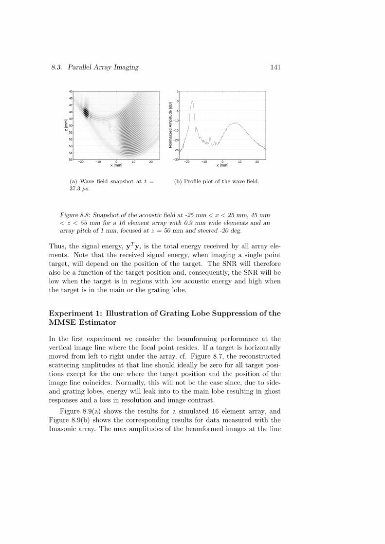
8.3. Parallel Array Imaging 141
x [mm]
z [m
m]
−20 −10 0 10 20
45
46
47
48
49
50
51
52
53
54
55
(a) Wave field snapshot at t =37.3 µs.
−20 −10 0 10 20−30
−25
−20
−15
−10
−5
0
5
x [mm]N
orm
aliz
ed A
mpl
itude
[dB
]
(b) Profile plot of the wave field.
Figure 8.8: Snapshot of the acoustic field at -25 mm < x < 25 mm, 45 mm< z < 55 mm for a 16 element array with 0.9 mm wide elements and anarray pitch of 1 mm, focused at z = 50 mm and steered -20 deg.
Thus, the signal energy, yTy, is the total energy received by all array ele-ments. Note that the received signal energy, when imaging a single pointtarget, will depend on the position of the target. The SNR will thereforealso be a function of the target position and, consequently, the SNR will below when the target is in regions with low acoustic energy and high whenthe target is in the main or the grating lobe.
Experiment 1: Illustration of Grating Lobe Suppression of the
MMSE Estimator
In the first experiment we consider the beamforming performance at thevertical image line where the focal point resides. If a target is horizontallymoved from left to right under the array, cf. Figure 8.7, the reconstructedscattering amplitudes at that line should ideally be zero for all target posi-tions except for the one where the target position and the position of theimage line coincides. Normally, this will not be the case since, due to side-and grating lobes, energy will leak into to the main lobe resulting in ghostresponses and a loss in resolution and image contrast.
Figure 8.9(a) shows the results for a simulated 16 element array, andFigure 8.9(b) shows the corresponding results for data measured with theImasonic array. The max amplitudes of the beamformed images at the line

142 Chapter 8. Applications
corresponding to the main lobe position, x = -18 mm, were plotted as afunction of the target position. The DAS beamformer used a fixed receivefocus at (z=50 mm, x = −18 mm), and the optimal filters for the corre-sponding image line were used in the MMSE estimator. In the simulations,the noise power was constant for all target positions where the SNR, definedby (8.14), was 15.8 dB when the target was at the focal point.
To show the influence of µ in (8.13), when µ is treated as a tuningparameter, the max amplitude was plotted as a function of the position ofa unit area point target for five values of µ: µ = 102, 103, 104, 106, and 109,respectively, see Figure 8.9(a). For low values of µ the MMSE filter reliesstrongly on the measured data, resulting in a significant noise amplification.This is seen in Figure 8.9(a), for µ = 102, where the noise floor only is about7 dB lower than the maximum amplitude at the focal point. Increasing µlowers the noise sensitivity but it also results in a worse suppression of thegrating lobe, which can be seen for µ = 106 and µ = 109. A good trade-offbetween the noise sensitivity and grating lobe suppression is in this caseµ = 104 where the noise and grating lobe levels are roughly 25 dB lowerthan the target signal. Note that the MMSE beamformer suppressed thegrating lobe better for all the examined µ values. It is also noticeable thatthe MMSE reconstructed image has higher lateral resolution than the DASbeamformed data.
A similar behavior can be seen in the experimental results, shown in Fig-ure 8.9(b), where µ = 102 was used for the MMSE estimates.10 Clearly, theresults from MMSE method show both higher resolution and a lower am-plitude at the grating lobe, even though model errors degraded the MMSEreconstructions somewhat.11
The fact the MMSE estimates becomes more similar to DAS beamformeddata for large values of µ, can be explained by the fact that the MMSEestimator reduces to a matched filter, PT /µ, when µ is large (cf. Section 5.4).Since the DAS beamformer approximately is a matched filter as well, theirperformance will be similar. Thus, if the variance of the measurement noiseis very high, then the MMSE estimator will reduce to a matched filter, whichis known to maximize the SNR.
From the results presented above it can be concluded that the MMSEestimator is capable of eliminating most of the grating lobe effects, if the
10µ = 102 resulted in the best visible performance.11The synchronization in the ALLIN system is sometimes inexact which introduces
modeling errors.
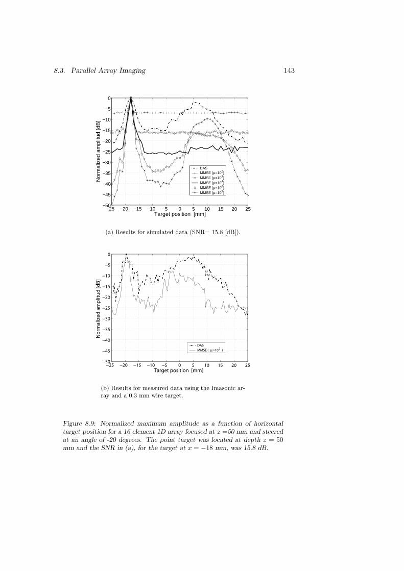
8.3. Parallel Array Imaging 143
−25 −20 −15 −10 −5 0 5 10 15 20 25−50
−45
−40
−35
−30
−25
−20
−15
−10
−5
0
Target position [mm]
Nor
mal
ized
am
plitu
d [d
B]
DASMMSE (µ=102)MMSE (µ=103)MMSE (µ=104)MMSE (µ=106)MMSE (µ=109)
(a) Results for simulated data (SNR= 15.8 [dB]).
−25 −20 −15 −10 −5 0 5 10 15 20 25−50
−45
−40
−35
−30
−25
−20
−15
−10
−5
0
Target position [mm]
No
rma
lize
d a
mp
litu
d [
dB
]
DAS
MMSE ( µ=102
)
(b) Results for measured data using the Imasonic ar-ray and a 0.3 mm wire target.
Figure 8.9: Normalized maximum amplitude as a function of horizontaltarget position for a 16 element 1D array focused at z =50 mm and steeredat an angle of -20 degrees. The point target was located at depth z = 50mm and the SNR in (a), for the target at x = −18 mm, was 15.8 dB.
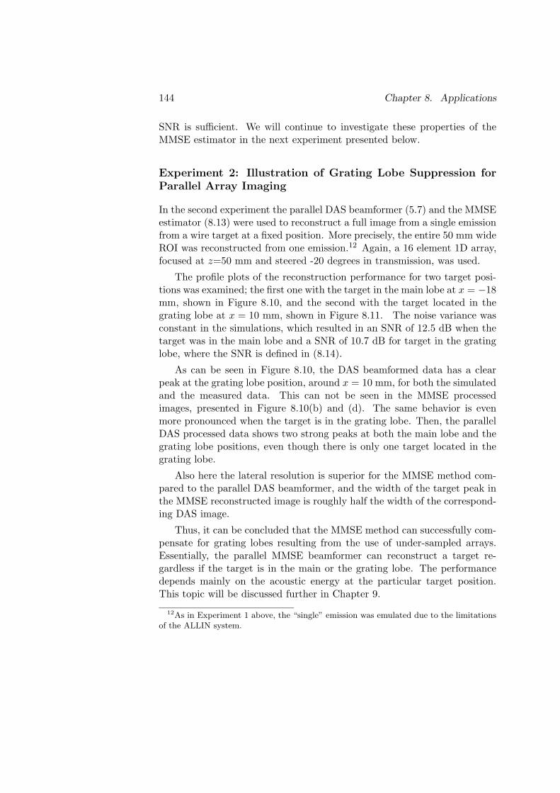
144 Chapter 8. Applications
SNR is sufficient. We will continue to investigate these properties of theMMSE estimator in the next experiment presented below.
Experiment 2: Illustration of Grating Lobe Suppression for
Parallel Array Imaging
In the second experiment the parallel DAS beamformer (5.7) and the MMSEestimator (8.13) were used to reconstruct a full image from a single emissionfrom a wire target at a fixed position. More precisely, the entire 50 mm wideROI was reconstructed from one emission.12 Again, a 16 element 1D array,focused at z=50 mm and steered -20 degrees in transmission, was used.
The profile plots of the reconstruction performance for two target posi-tions was examined; the first one with the target in the main lobe at x = −18mm, shown in Figure 8.10, and the second with the target located in thegrating lobe at x = 10 mm, shown in Figure 8.11. The noise variance wasconstant in the simulations, which resulted in an SNR of 12.5 dB when thetarget was in the main lobe and a SNR of 10.7 dB for target in the gratinglobe, where the SNR is defined in (8.14).
As can be seen in Figure 8.10, the DAS beamformed data has a clearpeak at the grating lobe position, around x = 10 mm, for both the simulatedand the measured data. This can not be seen in the MMSE processedimages, presented in Figure 8.10(b) and (d). The same behavior is evenmore pronounced when the target is in the grating lobe. Then, the parallelDAS processed data shows two strong peaks at both the main lobe and thegrating lobe positions, even though there is only one target located in thegrating lobe.
Also here the lateral resolution is superior for the MMSE method com-pared to the parallel DAS beamformer, and the width of the target peak inthe MMSE reconstructed image is roughly half the width of the correspond-ing DAS image.
Thus, it can be concluded that the MMSE method can successfully com-pensate for grating lobes resulting from the use of under-sampled arrays.Essentially, the parallel MMSE beamformer can reconstruct a target re-gardless if the target is in the main or the grating lobe. The performancedepends mainly on the acoustic energy at the particular target position.This topic will be discussed further in Chapter 9.
12As in Experiment 1 above, the “single” emission was emulated due to the limitationsof the ALLIN system.
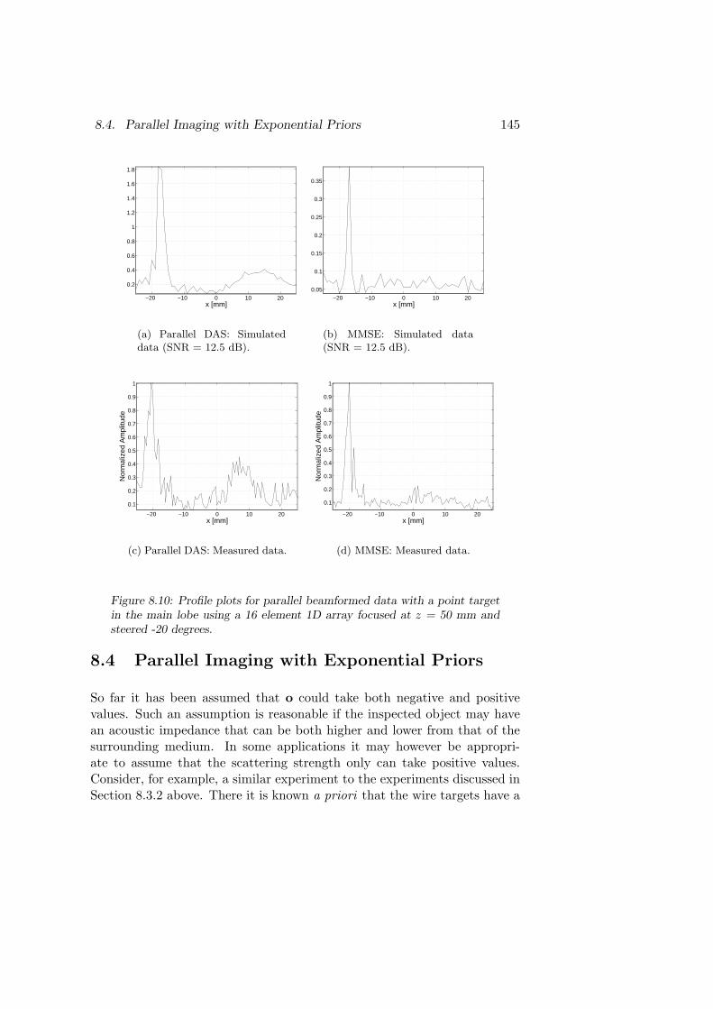
8.4. Parallel Imaging with Exponential Priors 145
−20 −10 0 10 20
0.2
0.4
0.6
0.8
1
1.2
1.4
1.6
1.8
x [mm]
(a) Parallel DAS: Simulateddata (SNR = 12.5 dB).
−20 −10 0 10 20
0.05
0.1
0.15
0.2
0.25
0.3
0.35
x [mm]
(b) MMSE: Simulated data(SNR = 12.5 dB).
−20 −10 0 10 20
0.1
0.2
0.3
0.4
0.5
0.6
0.7
0.8
0.9
1
x [mm]
Nor
mal
ized
Am
plitu
de
(c) Parallel DAS: Measured data.
−20 −10 0 10 20
0.1
0.2
0.3
0.4
0.5
0.6
0.7
0.8
0.9
1
x [mm]
Nor
mal
ized
Am
plitu
de
(d) MMSE: Measured data.
Figure 8.10: Profile plots for parallel beamformed data with a point targetin the main lobe using a 16 element 1D array focused at z = 50 mm andsteered -20 degrees.
8.4 Parallel Imaging with Exponential Priors
So far it has been assumed that o could take both negative and positivevalues. Such an assumption is reasonable if the inspected object may havean acoustic impedance that can be both higher and lower from that of thesurrounding medium. In some applications it may however be appropri-ate to assume that the scattering strength only can take positive values.Consider, for example, a similar experiment to the experiments discussed inSection 8.3.2 above. There it is known a priori that the wire targets have a

146 Chapter 8. Applications
−20 −10 0 10 20
0.1
0.2
0.3
0.4
0.5
0.6
0.7
0.8
0.9
x [mm]
(a) Parallel DAS: Simulateddata (SNR = 10.7 dB).
−20 −10 0 10 20
0.05
0.1
0.15
0.2
0.25
0.3
0.35
0.4
x [mm]
(b) MMSE: Simulated data(SNR = 10.7 dB).
−20 −10 0 10 20
0.1
0.2
0.3
0.4
0.5
0.6
0.7
0.8
0.9
1
x [mm]
Nor
mal
ized
Am
plitu
de
(c) Parallel DAS: Measured data.
−20 −10 0 10 20
0.1
0.2
0.3
0.4
0.5
0.6
0.7
0.8
0.9
1
x [mm]
Nor
mal
ized
Am
plitu
de
(d) MMSE: Measured data.
Figure 8.11: Profile plots for parallel beamformed images with a point targetin the grating lobe using a 16 element 1D array focused at z = 50 mm andsteered -20 degrees.
much higher acoustic impedance than the surrounding medium. Thus, theresulting scattering amplitude must be positive. By using this information,the reconstruction performance should be improved, especially for band lim-ited systems where linear deconvolution typically leads to ringings [38].
A drawback of imposing the positivity restriction on the scattering am-plitude is that a closed form expression for a MAP estimator can no longerbe found. This can be a serious drawback in ultrasonic array imaging appli-cations due to the usually high dimensionality in these problems. However,in some cases the MAP solution has a structure that enables the use of very

8.4. Parallel Imaging with Exponential Priors 147
efficient numerical methods. One such example is when the measurementnoise is Gaussian and the prior distribution for o is the exponential PDF.13
Recall from Section 7.1.3 that the MAP estimate for an exponential priorand Gaussian measurement noise can be found by solving the optimizationproblem
o = arg mino
1
2(y − Po)TCe
−1(y − Po) + λo1To
subject to oi ≥ 0 ∀i.
(8.16)
Eq. (8.16) is a quadratic programming (QP) problem with inequality con-straints. QP problems have the important property that they always canbe solved in a finite number of iterations, if a solution exists [85]. Here,the QP problem is convex since the Hessian matrix, PTC−1
e P is positivesemidefinite which further facilitates the solution of the problem.
The estimate obtained by solving (8.16) will hereafter be denoted thepositivity constrained quadratic programming, or PCQP, estimate. In thetwo experiments described below the PCQP estimate has been comparedwith the DAS beamformer, the matched filter (MF), and the linear MMSEestimator. The image to estimate consisted of about 5000 unknowns andall computations were performed, on as-of-today, standard PC hardware inless than an hour.
Below, the performance of the PCQP estimator is illustrated, using bothsimulated data and experimental data acquired using the Imasonic array.
Experiment 1: Focused Array using Simulated Data
In this experiment the PCQP estimate was compared with the parallel DASbeamformer, (5.7), the MMSE estimator, (8.13), and the matched filter,PT . The Imasonic array was simulated using 16 elements, focused at z = 50mm. A snapshot of the acoustic field around the focal point for this setupis shown in Figure 8.12. Since the array is under-sampled one can noticetwo grating lobes, at approximately x = ±23 mm, but most of the acousticenergy is focused around the center axis x = 0.
Three simulations were performed, with SNR = 30, 10, and -20 dB, werethe SNR is defined by (8.14). The true scattering image, o, had five pairs ofunit area point targets located at the horizontal positions x=-25, -13, 0, 13,
13The exponential PDF is also reasonable in the sense that it is the maximum entropydistribution if the mean is known as discussed in the previous chapter.

148 Chapter 8. Applications
x [mm]
z [m
m]
−20 −10 0 10 20
45
46
47
48
49
50
51
52
53
54
55
(a) Wave field snapshot at t =37.3 µs.
−20 −10 0 10 20−30
−25
−20
−15
−10
−5
0
5
x [mm]
Nor
mal
ized
Am
plitu
de [d
B]
(b) Profile plot of the wave field.
Figure 8.12: Snapshot of the acoustic field at -25 mm < x < 25 mm, 45mm < z < 55 mm for a 16 element array with 0.9 mm wide elements andan array pitch of 1mm focused at z = 50 mm.
and 25 mm, and vertically at z = 50 and z = 50.5 mm, respectively. Thevertical distance between the point targets is then roughly one wavelengthof the corresponding center frequency of the array.
To obtain a fair comparison we need to set the parameters in the MMSEand the PCQP so that the expected energy using both estimators is thesame. The prior that is determined by the mean value, λo, used in thePCQP estimator was based on the assumption that we can expect to findone unit area point target in the ROI. The mean scattered energy is thesum of the squared mean value and the variance, which for a single pointtarget becomes 12/MN = λ2
o + λ2o since the variance is given by λ2
o for theexponential PDF. Thus, λo is given by 1/
√2MN . By a similar reasoning the
variance, σ2o, used in the linear MMSE estimator is given by σ2
o = 1/MN .
The reconstruction results, for the respective SNRs, are displayed inFigures 8.13, 8.14, and 8.15. If we study the DAS and matched filter (MF)beamformed images it is evident that even for the data with the relativelyhigh SNR of 30 dB, shown in Figure 8.13, these two methods can onlyresolve the targets located close to the focal point. On the contrarym, theMMSE and PCQP estimators were able to resolve all targets. The PCQPestimator had, as it can be seen in 8.13(f), very low error in the scatteringamplitudes at all target positions. The MMSE estimator underestimated

8.4. Parallel Imaging with Exponential Priors 149t [
µs]
Receive element position x [mm]−7.5 −5 −2.5 0 2.5 5 7.5
35
40
45
50
55
60
65
70
(a) Simulated data (B-modeimage).
−7.5−5
−2.50
2.55
7.5
4050
6070
−0.1
−0.05
0
0.05
0.1
x [mm]t [µs]
(b) Simulated data.
−20−10
010
20
4547
4951
5355
−1
−0.5
0
0.5
1
x [mm]
Parallel delay−and−sum processed
z [mm]
(c) DAS.
−20−10
010
20
4547
4951
5355
−1−0.8−0.6−0.4−0.2
00.20.40.60.8
x [mm]
Matched Filter Processed Image
z [mm]
(d) Matched filter processedimage.
−20−10
010
20
4547
4951
5355
−0.2
0
0.2
0.4
0.6
0.8
x [mm]
MMSE Reconstructed Image
z [mm]
(e) MMSE.
−20−10
010
20
4547
4951
5355
0.2
0.4
0.6
0.8
x [mm]
Reconstructed Image w. Exponential Prior
z [mm]
(f) PCQP.
Figure 8.13: Simulated data, with an SNR of 30 dB for five pairs of pointtargets at x=-25, -13,0 13, and 25 mm, at z = 50 and z = 50.5 mm, re-spectively, and the reconstructions using the DAS, MF, MMSE, and PCQPalgorithms.

150 Chapter 8. Applications
the amplitudes somewhat in the regions where the acoustic power was low14,which is a reasonable behavior since the SNR in those regions is lower thanat the focusing region and the estimates are therefore more uncertain.
When decreasing the SNR to 10 dB the PCQP estimate, shown in Fig-ure 8.14, starts to show a similar behavior as the MMSE estimator, thatis, it becomes more “cautious” at regions with low acoustic power. This iseven more evident in the reconstructions from the rather low SNR of -20dB shown in Figure 8.15. Now, both the MMSE and PCQP estimatorsonly “trust” responses from the focusing region and all other responses areclose to zero. It is also noticeable that the MMSE reconstruction becomesmore similar to the MF output as the SNR decreases, see Figures 8.15(d)and (e). This is due to the fact, mentioned above, that the noise covari-ance matrix, Ce, dominates the factor (PCoP
T + Ce)−1 in the MMSE es-
timator when the SNR is low and the MMSE filter is then approximatelyKmmse ≈ σ2
oPT (σ2
eI)−1 = PT σ2
o/σ2e .
15
Noteworthy in Figure 8.15(f), is also the remarkable high ability of thePCQP estimator to suppress the measurement noise. Even though the re-ceived signals were completely hidden in the noise, see Figures 8.15(a) and(b), the PCQP estimator managed to predict the two targets at the focalpoint with a noticeable high contrast in the reconstructed image.
It is evident from these simulations that the two model based MMSEand PCQP methods are superior to traditional DAS based beamforming,in the sense that DAS processing does not perform well for targets outsidethe focusing region, whereas the two model based MMSE and PCQP meth-ods can reconstruct the targets with high temporal and lateral resolutionprovided that the SNR is sufficiently high.
Noticeable is also that, in contrast to the DAS and the MF beamformers,the overall amplitudes of the estimates become lower for both the MMSEand the PCQP estimators as the noise variance increases. In essence, thedata become less informative regarding the scattering amplitudes, o, whenthe noise variance increases and the MMSE and PCQP estimators thereforebecomes more cautious and underestimates the amplitudes.16 This is areasonable behavior which gives us a warning that the quality of the datamay not be sufficient for our particular purpose.
14The true target amplitude was 1 in this case.15The gain of the MMSE estimator is lower than that of the MF due to the factor σ2
o/σ2e ,
which will be low if the noise variance is high.16The amplitudes goes toward the a priori mean value, which was 0 for the MMSE
estimates and 1/√
2MN for the PCQP estimates in this case.

8.4. Parallel Imaging with Exponential Priors 151t [
µs]
Receive element position x [mm]−7.5 −5 −2.5 0 2.5 5 7.5
35
40
45
50
55
60
65
70
(a) Simulated data (B-modeimage).
−7.5−5
−2.50
2.55
7.5
4050
6070
−0.1
−0.05
0
0.05
0.1
x [mm]t [µs]
(b) Simulated data.
−20−10
010
20
4547
4951
5355
−1
−0.5
0
0.5
1
x [mm]
Parallel delay−and−sum processed
z [mm]
(c) DAS.
−20−10
010
20
4547
4951
5355
−1−0.8−0.6−0.4−0.2
00.20.40.60.8
x [mm]
Matched Filter Processed Image
z [mm]
(d) Matched filter processedimage.
−20−10
010
20
4547
4951
5355
−0.2
0
0.2
0.4
0.6
x [mm]
MMSE Reconstructed Image
z [mm]
(e) MMSE.
−20−10
010
20
4547
4951
5355
0.2
0.4
0.6
0.8
x [mm]
Reconstructed Image w. Exponential Prior
z [mm]
(f) PCQP.
Figure 8.14: Simulated data, with an SNR of 10 dB for five pairs of pointtargets at x=-25, -13,0 13, and 25 mm, at z = 50 and z = 50.5 mm, re-spectively, and the reconstructions using the DAS, MF, MMSE, and PCQPalgorithms.

152 Chapter 8. Applications
t [µs
]
Receive element position x [mm]−7.5 −5 −2.5 0 2.5 5 7.5
35
40
45
50
55
60
65
70
(a) Simulated data (B-modeimage).
−7.5−5
−2.50
2.55
7.5
4050
6070
−0.6
−0.4
−0.2
0
0.2
0.4
x [mm]t [µs]
(b) Simulated data.
−20−10
010
20
4547
4951
5355
−1
0
1
x [mm]
Parallel delay−and−sum processed
z [mm]
(c) DAS.
−20−10
010
20
4547
4951
5355
−1−0.8−0.6−0.4−0.2
00.20.40.60.8
x [mm]
Matched Filter Processed Image
z [mm]
(d) Matched filter processedimage.
−20−10
010
20
4547
4951
5355
−0.2
0
0.2
x [mm]
MMSE Reconstructed Image
z [mm]
(e) MMSE.
−20−10
010
20
4547
4951
5355
0.2
0.4
x [mm]
Reconstructed Image w. Exponential Prior
z [mm]
(f) PCQP.
Figure 8.15: Simulated data, with an SNR of -20 dB for five pairs of pointtargets at x=-25, -13,0 13, and 25 mm, at z = 50 and z = 50.5 mm, re-spectively, and the reconstructions using the DAS, MF, MMSE, and PCQPalgorithms.

8.4. Parallel Imaging with Exponential Priors 153
The general observation from these simulations is that it is the spatialdistribution of acoustic energy that is important for the reconstruction per-formance, not the actual pulse shape. More specifically, the reconstructionperformance of the model based methods employed here mostly depends onthe SNR in the particular region17 and not the length or shape of the wave-form. Moreover, as demonstrated above, the MMSE and PCQP estimatorscould estimate targets outside the focusing region, where the transmittedwaveforms from each element are not in phase, provided that the SNR wassufficient.
Experiment 2: Steered Array using Measured Data from Wire
Targets
To verify the above mentioned conclusions regarding the ability of the Baye-sian estimators to reconstruct targets outside the main beam, an experimentwith an under-sampled steered array is presented here. As we have men-tioned earlier, such an array will transmit energy both in the focusing di-rection and in the directions of the grating lobes. A relevant question istherefore if the Bayesian methods also are able to accurately estimate thescattering strength from a target located in a grating lobe?
For this purpose, the parallel DAS, MMSE and the PCQP methods wereused to reconstruct data from a 16 element array, focused at z = 50 andsteered at -20 degrees, acquired using the ALLIN system and the Imasonicarray. A snapshot of the resulting wave field from this setup is presentedin Figure 8.8 above. The measurements were performed using wire targets,positioned both in the main lobe at x = −18 mm and in the grating lobe atx = 10 mm, at depth z = 50 mm, see the illustration in Figure 8.16. Thereconstruction results are shown in Figure 8.17.
The results for the DAS method, shown in Figures 8.17(a) and (b),again demonstrate the typical leakage from the grating lobe associated withconventional beamforming. The temporal resolution for the DAS method isroughly the same as the length of the acoustic pulse for the target in themain lobe.18 Also, the temporal resolution for the target in the grating lobeis very poor which can be explained by the fact that the acoustic waveformis much longer in the grating lobe than at the focal point, see Figure 8.8(a).
As can be seen in Figures 8.17 (c)–(f), both the MMSE and the expo-
17The bandwidth of the system is also of importance [38].18This is expected since in ordinary DAS processing there is no compensation for the
transmitted pulse waveform.

154 Chapter 8. Applications
16 Element Array
Gratin
g lo
beM
ain
lob
e
Target position 1
Target position 2
Figure 8.16: Illustration of the measurement setup for Experiment 2. Theunder-sampled 16 element array was focused at z = 50 mm and steered -20degrees. A snapshot of the wave field for this configuration is presented inFigure 8.8.
nential MAP estimators suppressed the grating lobe well for both targetpositions, and the temporal resolution has also been improved compared toDAS processing. The MMSE estimates have however some ringing, see Fig-ure 8.17(d). This ringing behavior is most likely due to model errors causedby synchronization problems in the ALLIN array system. The PCQP esti-mates, shown in Figures 8.17(f) and (f), also have some extra “spikes” butthe amplitude of those spikes are smaller than the oscillations in the MMSEestimates.
Evidently, both of the model based MMSE and PCQP estimators wereable to accurately estimate the target strength, regardless if the wire targetwas located in the main or the grating lobe. This is in complete agreementwith the simulations in Experiment 1 above.
The results from the two experiments presented in this section showsthat, at least for high contrast targets, the use of an exponential prior PDFfor the scattering amplitudes can give impressive results with very high tem-poral and lateral resolution. The contrast is also very high and the noise levelin the reconstructions are often very low. The remarkable performance ofthe exponential MAP estimator is due to the correct prior information thatwas incorporated into the model, which enables the estimator to effectivelydiscriminate between noise and the target responses.

8.4. Parallel Imaging with Exponential Priors 155
−20−10
010
20
4547
4951
53
−1
−0.5
0
0.5
1
x [mm]
Parallel delay−and−sum processed
z [mm]
Nor
mal
ized
Am
plitu
de
(a) DAS: Target in main lobe.
−20−10
010
20
4547
4951
53
−1
−0.5
0
0.5
1
x [mm]
Parallel delay−and−sum processed
z [mm]
Nor
mal
ized
Am
plitu
de
(b) DAS: Target in gratinglobe.
−20−10
010
20
4547
4951
53
−0.5
0
0.5
1
x [mm]
MMSE Reconstructed Image
z [mm]
Nor
mal
ized
Am
plitu
de
(c) MMSE: Target in mainlobe.
−20−10
010
20
4547
4951
53
−0.5
0
0.5
1
x [mm]
MMSE Reconstructed Image
z [mm]
Nor
mal
ized
Am
plitu
de
(d) MMSE: Target in gratinglobe.
−20−10
010
20
4547
4951
53
0.2
0.4
0.6
0.8
1
x [mm]
Reconstructed Image w. Exponential Prior
z [mm]
Nor
mal
ized
Am
plitu
de
(e) PCQP: Target in mainlobe.
−20−10
010
20
4547
4951
53
0.2
0.4
0.6
0.8
1
x [mm]
Reconstructed Image w. Exponential Prior
z [mm]
Nor
mal
ized
Am
plitu
de
(f) PCQP: Target in gratinglobe.
Figure 8.17: Reconstructions from measured data using a wire target in themain lobe (Figs. (a), (c), and (e)) and a wire target in the grating lobe(Figs. (b), (d), and (f)). The data were acquired using the ALLIN systemand the concave Imasonic array. The transmit beam was steered at -20 degand focused at 50 mm using 16 array elements.
156 Chapter 8. Applications
The most significant drawback of the PCQP method is that the estimatemust be obtain by an iterative optimization algorithm. This makes themethod most suitable for offline processing where real-time constraints areof little concern.
8.4.1 Remarks
Focusing phase errors: The transmit focusing delays in ultrasonic arrayimaging systems are often subject to quantization errors. This re-sults in a slightly different transmit beampattern then the desired.In classical beamforming this will result in increased sidelobe ampli-tudes [16, 90]. However, the model based estimators discussed herecan compensate for these errors given that the true focusing delaysare known.
Correlated scattering: In the experiments discussed in this chapter itwas assumed that the scattering amplitudes at all image points wereuncorrelated. In some applications the scattering objects can, for ex-ample, have a layered structure (e.g., in seismic exploration) resultingin correlations between the scatterers. This knowledge can be easilyintroduced in the linear MMSE estimator by means of the covariancematrix Co.
Priors: In the experiments performed with the ALLIN system presented inthis chapter the a priori mean and variance of the scattering strengthwere in reality unknown. Despite this fact, we have seen in the resultsfrom both the linear MMSE and the non-linear PCQP method thatthe exact mean or variance are not required. Our experience is thatthe reconstruction results for both these model based methods are notsensitive to the particular value of the variance or the mean. Thevariance or mean can typically be changed by a factor of 10 withoutsignificantly affect the reconstruction performance. Furthermore, it ispossible to design an experiment, with a known set of scatterers, toestimate the unknown quantities. However, this is a topic for futureresearch.
8.5 Summary
In this chapter we have evaluated performance of the linear MMSE estimatorand the PCQP estimator used for the reconstruction of ultrasonic data in

8.5. Summary 157
monostatic configuration as well as in multistatic parallel array imaging.
It was demonstrated that both estimators were capable of reconstructingmultiple targets with high accuracy in the experiments even if the ultrasonicdata were sparsely sampled. However, the PCQP estimator were more im-mune to the corrupting noise.
The MMSE estimator, which in the simplest case results in a spatio-temporal filter with only one scalar tuning parameter, clearly outperformedtraditionally used DAS beamforming algorithms in terms of higher resolutionboth for the targets in water and in an immersed solid. In the parallel receiveimaging, the MMSE algorithm clearly minimized target leakage from thegrating lobes and could be successfully used for correct reconstruction oftargets located in the grating lobes.
However, when our prior information tells us that the scattering strengthalways is positive the best performance was achieved using the nonlinearPCQP estimator developed for the exponential prior. This estimator clearlyoutperformed the linear MMSE estimators in terms of high immunity tothe measurement noise and its ability to reconstruct multiple targets in theROI.
The performance of the proposed estimators is achieved at the price ofthe increased computational complexity, especially, for the PCQP algorithmwhich takes the form of an iterative optimization algorithm.

158 Chapter 8. Applications

CHAPTER 9
Performance of the Optimal Linear Estimator
IN this chapter we turn the attention to the influence that the array systemdesign has on reconstruction performance and, in particular, how we can
evaluate different array layouts. Traditionally, array systems are designedwith classical beamforming in mind, meaning that the design of the ar-ray system must respect the limitations that classical beamfoming imposes.Namely, sub-wavelength array pitches and small element sizes in order toavoid artifacts and resolution loss. The Bayesian estimators, presented ear-lier in this thesis, do however not not impose these restrictions and a moreflexible array design should therefore be possible.
The aim of this chapter is to show that Bayesian analysis offer a usefultool for designing and evaluating ultrasonic array systems. This is due tothe fact that these methods provides a natural measure of the accuracy ofthe estimates. According to the discussion in Section 7.1, the performanceof the optimal linear estimator is given by the error covariance matrix, Cε,in (7.11), which can be analyzed for different array layouts.
In this chapter we will show that, for the linear MMSE estimator, theexpected mean-squared error can give us valuable information regarding,in particular, the choice of suitable focusing strategies. In agreement withcommon sence, it will be demonstrated that focused beams are needed ifthe noise is high to obtain a sufficiently low expected error at least in thelimited region of the main beam.
This chapter is organized as follows: In Section 9.1, we present an ex-
159

160 Chapter 9. Performance of the Optimal Linear Estimator
pression for the normalized expected error which is then used in Section 9.2,to evaluate the performance for three parallel array imaging setups.
9.1 The Normalized Expected Error
Recall from Chapter 7 that, for the linear MMSE estimator (7.7), the dis-tribution for the reconstruction error, ε = ommse − o, is Gaussian if themeasurement noise and the prior are both Gaussian. The expected mean-squared error at each observation point are given by the diagonal elementsof the error covariance matrix Cε. The performance of the MMSE estimatorcan then be evaluated by organizing the diagonal elements diag{Cε} intoan M ×N error image Eε. Below, we present a normalized error covariancematrix for the purpose of facilitating the comparison of different transmitfocusing methods.
The error covariance matrix is given by (cf. Appendix 7.A.2)
Cε = Co − CoPT (PCoP
T + Ce)−1PCo
= (C−1o + PTC−1
e P)−1.(9.1)
Let us consider a special case where Co = σ2oI and Ce = σ2
eI. Then theerror covariance matrix Cε becomes
Cε = σ2oI − σ2
oPT (σ2
oPPT + σ2eI)
−1Pσ2o
= (I/σ2o + PTP/σ2
e )−1.
(9.2)
If we now normalize (7.67) with respect to σ2o, then the normalized error
covariance matrix becomes
Cε =1
σ2o
Cε
= I − PT (σ2oPPT + σ2
eI)−1Pσ2
o
= (I + PTPσ2o/σ
2e )
−1.
(9.3)
If σ2e is very large compared to PTPσ2
o, then the normalized error co-variance matrix will reduce to the identity matrix which is the worst casescenario where the data holds no new information. A region in the normal-ized error image, Eε consisting of the diagonal elements of Cε with a valueclose to unity will then indicate poor reconstruction performance in thatregion.

9.2. Parallel Array Imaging Performance 161
In the next section we will utilize Eε to evaluate the performance of thelinear MMSE estimator for a simulated phased array.1
9.2 Parallel Array Imaging Performance
To illustrate the performance of the parallel MMSE estimator (8.13), withrespect to focusing method and SNR, three example array setups are con-sidered. In all tree setups the Imasonic array described in Section 8.1 wassimulated and 16 array elements are used in receive mode. The transmitbeam is focused in tree different ways as illustrated in Figure 9.1.
16 Element Linear Array
(a) 16 transmitelements focusedarray.
16 Element Linear ArrayG
rating
lob
eMai
n lo
be
(b) 16 transmit elementssteered array.
16 Element Linear Array
(c) One transmit ele-ment.
Figure 9.1: Illustration of the transmit focusing methods for the simulationspresented in Figures 9.2–9.4.
1. The beam is focused at z = 50 mm with no beam steering.
2. The beam is focused and steered -20 deg resulting in a focal point atx = −18, z = 50 mm.
3. One single element was used in transmit mode.
1The array was simulated using the DREAM toolbox.

162 Chapter 9. Performance of the Optimal Linear Estimator
The first two setups, where the array is focused, result in regions with bothhigh and low acoustic energy. The third setup, where a single element isused, results in a wider beam illuminating more of the ROI but the totaltransmitted acoustic energy will be lower. The reason for the lower transmitpower is that by only using one element the active area of the transmitaperture is reduced by a factor 1/16 compared to the other two setups.
Normalized error images, obtained using (9.3) and the three focusingmethods, are shown in Figures 9.2, 9.3, and 9.4, respectively. The noisevariance σ2
e is highest in Figure 9.2 and lowest in Figure 9.4 and the ratio,σ2
e/σ2o, in the respective figures are 2.5 · 10−3, 2.5 · 10−5, and 2.5 · 10−8.
The error images presented in Figure 9.2 correspond to a very low SNR.It can clearly be seen in Figures 9.2(a) and (b) that the normalized error willonly deviate from unity at those image points that are in the vicinity of afocal point or a grating lobe, that is, at those points where most of the energyis transmitted. It can also be seen that the error at the focal point is lowerfor the array that is not steered, even though the same number of elementsare used in transmit mode for the steered array. This can be explained byconsidering the beam directivity of an individual array element as discussedin Section 6.2. An array element of the Imasonic array has a width ofapproximately 2λ at the array’s center frequency, and the element’s beamdirectivity can therefore not be neglected. The array element will transmitmost energy in the normal direction of its active surface area where theSIRs are shortest, as discussed in Chapter 3. At high angles, the SIRs willattenuate the signal, especially for the higher frequencies. Elements that arehorizontally closer to the focal point will, therefore, contribute more thanthe ones further away from the focal point. Steering at high angles will thenessentially reduce the effective number of transmit elements due to the beamdirectivity of the array elements. In fact, it can be seen in Figure 9.2(b) thatthe error is of the same order both in the main- and grating lobe for thesteered array. The reason for this behavior is that the grating lobe is closerto the array center than the main lobe and more elements will thereforecontribute to the acoustic field.
It can also be seen in Figure 9.2(c) that the acoustic power from oneelement was not sufficient at this SNR since the normalized error was closeto unity at all image points.
If the noise level is decreased then the estimation error will also de-crease. The noise level in Figure 9.3 is 20 dB lower than in Figure 9.2 andthe normalized error has been substantially decreased for all three trans-


166 Chapter 9. Performance of the Optimal Linear Estimator
CHAPTER 10
Concluding Remarks and Future Research
The classical approach to ultrasonic imaging using arrays is inspired bygeometrical optics and consists in designing discrete versions of lens systemscapable of focusing and steering ultrasonic beams.
In the new approach to ultrasonic imaging presented in this work the ul-trasonic image reconstruction was formulated as a linearized inverse-scatteringproblem taking into account both the discrete nature of the imaging setupas well as the modeling errors. This formulation has enabled global opti-mization of the imaging performance given the a priori information on theimaging system parameters and the PDF’s of errors and scatterers present inROI. Although the optimization in this work was performed in terms of reso-lution, given the parameters, such as, transducer size, its electro-mechanicalcharacteristics and the exciting waveform it is also possible to include theseparameters in the optimization process. This creates the possibility of opti-mizing transducer’s bandwidth and the form of its exciting signal accordingto the imaging performance to achieve a global optimum of the imagingprocess.
The estimation was performed by means of the tools from Bayesian esti-mation theory using the specially developed for this purpose linear discretematrix model of the imaging system. It is known from statistics that theMAP approach leads to analytic solutions only for a very few PDF fami-lies, in most cases the optimization of the a posteriori probability has to beperformed numerically.
167
168 Chapter 10. Concluding Remarks and Future Research
In the work the measurement errors were assumed to be Gaussian, andtwo special prior distributions of scatterers were considered, Gaussian andexponential.
It was shown that for Gaussian PDF’s the MAP approach results inthe MMSE criterion. The linear MMSE solution takes the form of a lin-ear spatio-temporal filter which deconvolves the distortion caused by thediffraction effects of the transducer used for imaging using the informationcontained in the transducer’s SIRs.
For the exponential PDF of scatterers in the ROI the solution was formu-lated as a nonlinear optimization problem with constrains which was solvednumerically.
The imaging algorithms resulting from the proposed approach were ver-ified using simulated and real ultrasonic data. The algorithms are of generalcharacter and can be applied both to the synthetic aperture imaging (mono-static and bistatic) as well as to the parallel beamforming.
It was demonstrated that the linear MMSE and the nonlinear PCQPestimators were superior to the classical beamforming in terms of resolutionand sidelobe level.
It should be noted however, that the successive application of the pro-posed approach relies on the reliable information concerning the imagingsetup, transducer’s SIRs as well as the statistics of the measurement noiseand the scatterers present in ROI. In our experiments the SIRs calculatednumerically for given setup and the transducer geometry were successfullyused. The statistics were not estimated explicitly but found using the trial-and-error method for the particular ultrasonic data.
Future Research
Model size reduction: The propagation matrix P in (4.23) is inherentlylarge if the ROI is densely sampled. In many applications there areonly a few scatterers, or the scatterers are confined to a localized area.In such situations many of the observation points will not contributeto the measurement y. If this is known in advance the matrix P canbe truncated resulting in a much smaller problem. If the location ofthe targets is not known in advance one needs a “zooming” strategyto find areas where the sampling needs to be dense.
Prior: Assumptions concerning the prior are needed for the model based

169
imaging algorithms. Since little is known about scatterers’ statisticsexperiments with a set of known objects yielding reliable estimates ofthe mean and variance should be performed.
Optimal input signal design: The choice of input signal driving the ul-trasonic array elements is fundamental in the sense that it may deter-mine the reconstruction accuracy [91, 92]. The input signals commonlyused in ultrasonic imaging, such as, tone-burst or impulse excitationmay not be the optimal choice with respect to reconstruction per-formance. Since the developed linear model takes into account theinput signal, the reconstruction algorithms based on the model willautomatically compensate for the chosen input signal. In effect the re-construction performance can be optimized with respect to the inputsignal. Therefore developing feasible methods for designing suitableinput signals for the particular ultrasonic array imaging applicationsis of great interest [93].
Parallel implementations: The matrix based models are inherently largeand therefore, the image reconstruction, that generally results in solv-ing linear equation systems or solving (constrained) optimization prob-lems, also results in large equation sets. To be able to scale up theseproblems and improve computation time it is desirable to distributethe computation on parallel computers.
Sparse arrays: Sparse arrays are used in 3D medical applications. Perfor-mance of the proposed algorithms should be experimentally verifiedfor such arrays.

170 Chapter 10. Concluding Remarks and Future Research

BIBLIOGRAPHY
[1] S.L. Bridal, J-M. Correras, A. Saıed, and P. Laugier. Milestones on theroad to higher resolution, quantative, and functional imaging. Proceed-
ings of the IEEE, 91(10):1543–1561, 2003.
[2] O.T. von Ramm and S.W. Smith. Beam steering with linear arrays.IEEE Transactions on Biomedical Engeering, 30:438–452, August 1983.
[3] K.E. Thomenious. Evaluation of ultrasound beamformers. In IEEE
Ultrasonics Symposium, 1996.
[4] H. Krim and M. Viberg. Two decades of array signal processing re-search. IEEE Signal Processing Magasine, pages 67–94, July 1996.
[5] J.A. Seydel. Ultrasonic synthetic-aperture focusing techniques in NDT.Research Techniques for Nondestructive Testing. Academic Press, 1982.
[6] S.R. Doctor, T.E. Hall, and L.D. Reid. SAFT—the evolution of asignal processing technology for ultrasonic testing. NDT International,19(3):163–172, June 1986.
[7] K.J. Langenberg, M. Berger, Th. Kreutter, and V. Mayer,K.and Schmitz. Synthetic aperture focusing technique signal process-ing. NDT International, (3):177–189, June 1986.
[8] M. Karman and M. O’Donnell. Synthetic aperture imaging for smallscale systems. IEEE Transactions on Ultrasonics, Ferroelectrics, and
Frequency Control, 42(3):429–442, May 1995.
171

172 BIBLIOGRAPHY
[9] G.S. Kino. Acoustic Waves: Devices, Imaging and Analog Signal Pro-
cessing, volume 6 of Prentice-Hall Signal Processing Series. Prentice-Hall, 1987.
[10] L.W. Schmerr, Jr. Fundamentals of Ultrasonic Nondestructive Evalua-
tion: A Modeling Approach. Plenum Press, 1998.
[11] J. Krautkramer and K. Krautkramer. Ultrasonic Testing of Materials.Springer-Verlag, 1990.
[12] J.A. Ogilvy and J.A.G. Temple. Diffraction of elastic waves by cracks:application to time-of-flight inspection. Ultrasonics, pages 259–269,Nowember 1983.
[13] B.R. Tittmann. Scattering of elastic waves from simple defects in solids,a review. Wave Motion, 1983.
[14] M.G. Silk. Changes in ultrasonic defect location and sizing. NDT
International, 20(1), February 1987.
[15] P.D. Corl, G.S. Kino, C.S. DeSilets, and P.M. Grant. A digital syntheticfocus acoustic imaging system. Acoustical Imaging, pages 39–53, 1980.
[16] B.D. Steinberg. Digital beamforming in ultrasound. IEEE Transactions
on Ultrasonics, Ferroelectrics, and Frequency Control, 39(6):716–721,November 1992.
[17] J.W. Goodman. Introduction to Fourier Optics. McGraw-Hill, secondedition, 1996.
[18] R.N. Thomson. Transverse and longitudinal resolution of the syntheticaperture focusing technique. Ultrasonics, 22(1):9–15, January 1984.
[19] H. Lee and G. Wade. Constructing an imaging operator to enhanceresolution. Journal of the Acoustical Society of America, 75(2):499–504, February 1984.
[20] H. Lee. Resolution enhancement by wavefield extrapolation. IEEE
Transactions on Sonics and Ultrasonics, (6):642–645, 1984.
[21] R. Stoughton. Optimal near-field measurement in the prescence of noiseand reflections. Journal of the Acoustical Society of America, 92(2):831–840, August 1992.

BIBLIOGRAPHY 173
[22] R. Stoughton. Source imaging with minimum mean-squared error.Journal of the Acoustical Society of America, 94(2):827–834, Aug 1993.
[23] S. Strait and R. Stoughton. Source imaging with minimum mean-squared error. Journal of the Acoustical Society of America, 94(2):827–834, August 1993.
[24] S.K. Lehman and A.J. Devaney. Transmission mode time-reversalsuper-resolution imaging. Journal of the Acoustical Society of America,113(5):2742–2753, May 2003.
[25] P. Blomgren and G. Papanicolaou. Super-resolution in time-reversalacoustics. Journal of the Acoustical Society of America, 111(1):230–248, January 2002.
[26] A.A. Aydiner and W.C. Chew. On the nature of super-resolution ininverse scattering. In IEEE Antennas and Propagation Society, AP-S
International Symposium, pages 507–510, 2003.
[27] A.J. Willis and R. De Mello Koch. A linear reconstructive approach tosuper-resolution array processing. Journal of the Acoustical Society of
America, 97(5):3002–3005, May 1995.
[28] C. Prada and J-L. Thomas. Experimantal subwavelength localizationof scatterers by decomposition of the time reversal operator intepretedas a covariance matrix. Journal of the Acoustical Society of America,114(1):235–243, 2003.
[29] E. T. Jaynes. Detection of extra-solar-system planets. In Maximum-
Entropy and Bayesian Methods in Science and Engineering. Kluwer,Dordrecht, 1988.
[30] K.L. Gammelmark and J.A. Jensen. Multielement synthetic transmitaperture imaging using temporal encoding. IEEE Transactions on Med-
ical Imaging, 22(4):552–563, April 2003.
[31] G. Demoment. Image reconctruction and restoration: Overview ofcommon estimation structures and problems. IEEE Transactions on
Acoustics, Speech, and Signal Processing, 42:1024–2036, Dec 1989.
[32] P.N.T. Wells. Ultrasonics: a window into biomedical science. Ultrason-
ics, 30(1):3–7, 1992.
[33] M. Soumekh. Fourier Array Imaging. Prentice Hall, 1994.

174 BIBLIOGRAPHY
[34] B.R. Mahafza. Radar Systems Analysis and Design Using MATLAB.Chapman & Hall/CRC, 2000.
[35] P. de Heering. Alternate schemes in synthetic aperture sonar processing.IEEE Journal of Oceanic Engineering, 9(4):277–280, October 1984.
[36] P.T. Gough and D.W. Hawkins. Imaging algorithms for strip-map syn-thetic aperture sonar: Minimizing the effects of aperure errors andaperture undersampling. IEEE Journal of Oceanic Engineering, 22:27–39, January 1997.
[37] B. Haider, P.A. Levin, and K. Thomenious. Pulse elongation and decon-volution filtering for medical ultrasonic imaging. In IEEE Ultrasonics
Symposium, pages 1303–1308, 1995.
[38] T. Olofsson. Maximum A Posteriori Deconvolution of Ultrasonic Data
with Applications in Nondestructive Testing. PhD thesis, Uppsala Uni-versity, Uppsala, Sweden, 2000.
[39] M. Fatemi and A.C. Kak. Ultrasonic B-scan imaging: theory of imageformation and a technique for restoration. Ultrasonic Imaging, 2:1–47,1980.
[40] S.F. Burch. Comparison of SAFT and two-dimensional deconvolutionmethods for the improvement of resolution in ultrasonic B-scan images.Ultrasonics, 25(4):259–266, 1987.
[41] A. Herment, J.P. Guglielmi, P. Dumee, P. Peronneau, and P. Delouche.Limitations of ultrasound imaging and image restoration. Ultrasonics,25(5):267–273, September 1987.
[42] T. Taxt. Restoration of medical ultrasound images using two-dimensional homomorphic deconvolution. IEEE Transactions on
Ultrasonics, Ferroelectrics, and Frequency Control, 42(4):543–544, July1995.
[43] M. Tanter, J-L. Thomas, and M. Fink. Time reversal and the inversefilter. Journal of the Acoustical Society of America, pages 223–234, July2000.
[44] M. Tanter, J.-F. Aubry, J. Gerber, J.-L. Thomas, and M. Fink. Optimalfocusing by spatio-temporal inverse filter. I. Basic principles. Journal
of the Acoustical Society of America, pages 37–47, July 2001.

BIBLIOGRAPHY 175
[45] O.S. Haddadin and E.S. Ebbini. Ultrasonic focusing through inhomoge-neous media by application of the inverse scattering problem. Journal
of the Acoustical Society of America, 104(1):313–325, July 1998.
[46] P.M. Morse and K.U. Ingard. Theoretical Acoustics. 1968.
[47] J.D. Logan. Applied Mathematics. Wiley, second edition, 1997.
[48] P.M. Morse and H. Feshbach. Methods of Theoretical Physics: Part I.McGraw-Hill, 1953.
[49] H. Lasota, R. Salamon, and B. Delannoy. Acoustic diffraction analysisby the impulse response method: A line impulse response approach.Journal of the Acoustical Society of America, 76(1):280–290, July 1984.
[50] J.W.S. Rayleigh. The Theory of Sound, volume 2. New York: Dover,1945.
[51] B. Delannoy, H. Lasota, C. Bruneel, R. Torguet, and E. Bridoux. Theinfinite planar baffles problem in acoustic radiation and its experimentalverification. Journal of Applied Physics, 50(8):5189–5195, August 1970.
[52] B. Piwakowski and B. Delannoy. Method for computing spatial pulseresponse: Time-domain approach. Journal of the Acoustical Society of
America, 86(6):2422–32, Dec 1989.
[53] B. Piwakowski and K. Sbai. A new approach to calculate the fieldradiated from arbitrarily structured transducer arrays. IEEE Transac-
tions on Ultrasonics, Ferroelectrics, and Frequency Control, 46(2):422–40, 1999.
[54] A. Lhemery. Impulse-response method to predict echo-responses fromtargets of complex geometry. Part I: Theory. Journal of the Acoustical
Society of America, pages 2799–2807, November 1991.
[55] H. Lasota and R. Salamon. Application of time-space impulse responsesto calculations of acoustic field in imaging systems. Acoustic Imaging,pages 493–512, 1980.
[56] P.R. Stepanishen. Transient radiation fom pistons in an infinite planarbaffle. Journal of the Acoustical Society of America, 49:1629–38, 1971.
[57] J.C. Lockwood and J.G. Willette. High-speed method for computingthe exact solution for the pressure variations in the nearfield of a baffled

176 BIBLIOGRAPHY
piston. Journal of the Acoustical Society of America, 53(3):735–741,March 1973.
[58] C.A. Wiley. Synthetic aperture radars. IEEE Transactions on
Aerospace and Electronic Systems, 21:440–443, 1985.
[59] C.W. Sherwin, J.P. Ruina, and R.D. Rawcliffe. Some early develop-ments in synthetic aperture radar systems. IRE Transactions Military
Electronics, 6:111–115, April 1962.
[60] K.D. Rolt and H. Schmidt. Azimultal ambiguities in synthetic aperturesonar and synthetic radar imagery. IEEE Journal of Oceanic Engineer-
ing, 17(1):73–79, January 1992.
[61] S.I. Nikolov and J.A. Jensen. 3D synthetic aperture imaging usinga virtual source element in the elevation plane. In IEEE Ultrasonics
Symposium, 2000.
[62] C.H. Frazier and Jr. W.D. O’Brien. Synthetic aperture techniqueswith a virtual source element. IEEE Transactions on Ultrasonics,
Ferroelectrics, and Frequency Control, 45(1):196–207, January 1998.
[63] M-H. Bae and M-K. Jeong. A study of synthetic-aperture imagingwith virtual source elements in B-mode ultrasound imaging systems.IEEE Transactions on Ultrasonics, Ferroelectrics, and Frequency Con-
trol, 47(6):1510–1519, November 2000.
[64] D. Vray, C. Haas, T. Rastello, M. Krueger, E. Busseau, K. Schroeder,G. Gimenez, and H. Ermert. Synthetic aperture-based beam com-pression for intravascular ultrasound imaging. IEEE Transactions on
Ultrasonics, Ferroelectrics, and Frequency Control, 48(1):189–201, Jan-uary 2001.
[65] C. Passman and H. Ermert. A 100MHz ultrasound imaging system fordermatologic and ophthalmologic diagnostics. IEEE Transactions on
Ultrasonics, Ferroelectrics, and Frequency Control, 43(4):545–552, July1996.
[66] M. O’Donnell and L.J. Thomas. Efficient synthetic aperture imagingfrom a circular aperture with possible application to catheter-basedimaging. IEEE Transactions on Ultrasonics, Ferroelectrics, and Fre-
quency Control, 39(3), May 1992.

BIBLIOGRAPHY 177
[67] K. Nagai. A new synthetic-aperture focusing method for ultrasonic B-scan imaging by the Fourier transform. IEEE Transactions on Sonics
and Ultrasonics, 32(4):531–536, July 1985.
[68] K. Mayer, R. Marklein, K.J. Langenberg, and T. Kreutter. Three-dimensional imaging system based on fourier transform synthetic aper-ture focusing technique. Ultrasonics, 28:241–255, July 1990.
[69] M. Lorenz. Ultrasonic Imaging for the Characterization of Defects in
Steel Components. PhD thesis, Delft University of Technology, 1993.
[70] R. Hannemann. Modeling and Imaging of Elastodynamic Wave Fields
in Homogenous Anisotropic Media. PhD thesis, Kassel University, 2001.
[71] S. Nikolov. Synthetic Aperture Tissue and Flow Ultrasonic Imaging.PhD thesis, Technical University of Denmark, 2001.
[72] J. Chatillon, M.E. Bouhier, and M.E. Zakharia. Synthetic aperturesonar for seabed imaging: relative merits of narrow-band and wide-band approached. IEEE Journal of Oceanic Engineering, 17(1):95–105,Jan 1992.
[73] J.A. Cadzow. Matched filters. In Foundations of Digital Signal Pro-
cessing and Data Analysis, pages 442–461. Macmillan, NY, 1987.
[74] G.L. Turin. An introduction to matched filters. IRE Transactions on
Information Theory, 6(3):311–329, 1960.
[75] C. Dorme and M. Fink. Focusing in the transmit-receive mode throughinhomogeneous media: The matched filter approach. Journal of the
Acoustical Society of America, 98:1155–1161, 1995.
[76] M. Fink. Time-reversal mirrors. Journal of Applied Physics, 26:1333–1350, 1993.
[77] J. Shen and E. Ebbini. A new coded-excitation ultrasonic imagingsystem—Part I: Basic principles. IEEE Transactions on Ultrasonics,
Ferroelectrics, and Frequency Control, 43(1), January 1996.
[78] S.-C. Wooh and Y. Shi. Influence of phased array element size on beamsteering behavior. Ultrasonics, 36:737–749, 1998.
[79] D.P. Shattuck, M.D. Weinshenker, S.W. Smith, and O.T. von Ramm.Explososcan: a parallel processing technique for high speed ultrasound

178 BIBLIOGRAPHY
imaging with linear phased arrays. Journal of the Acoustical Society of
America, 75(4):1273–1282, April 1984.
[80] O.T. von Ram, S.W. Smith, and H.G. Pavy Jr. High-speed ultrasoundvolumetric imaging system. II. Parallel processing and image display.IEEE Transactions on Ultrasonics, Ferroelectrics, and Frequency Con-
trol, 38(2):109–15, March 1991.
[81] T.M. Cover and J.A. Thomas. Elements of Information Theory. Wiley,1991.
[82] E.T. Jaynes. Probability Theory: The Logic of Science. CambridgeUniversiy Press, 1st edition, 2003.
[83] W.R. Gilks, S. Richardson, and D.J. Spieglhalter. Markov Chain Monte
Carlo in Practice. Chapman & Hall/CRC, 1996.
[84] S.M. Kay. Fundamantals of Statistical Signal Processing: Estimation
Theory, volume I. Prentice Hall, 1993.
[85] J. Nocetal and S.J. Wright. Numerical Optimization. Springer-Verlag,1999.
[86] G. Strang. Linear Algebra and its Applications. Sounders HBJ, 1986.
[87] A. Tikonov and V. Arsenin. Solutions of Ill-Posed Problems. WinstonWashington DC, 1977.
[88] T. Soderstrom. Discrete-Time Stochastic Systems: Estimation & Con-
trol. Prentice Hall International, 1994.
[89] B. Delannoy, R. Toutguet, C. Bruneel, E. Bridoux, J.M. Rouvaen, andH. Lasota. Acoustical image reconstruction in parallel-processing ana-log electronic systems. Journal of Applied Physics, 50(5):3153–3159,May 1979.
[90] S. Holm. Analysis of worst-case phase quantization sidelobes in focusedbeamforming. IEEE Transactions on Ultrasonics, Ferroelectrics, and
Frequency Control, 39(5):593–599, September 1992.
[91] R.K. Mehra. Optimal input signals for parameter estimation in dynam-ical systems—survey and new results. IEEE Transactions on Automatic
Control, (6):753–768, Dec 1974.

BIBLIOGRAPHY 179
[92] S.M. Sowelam and A.H. Tewfik. Waveform selection in radar targetclassification. Transactions on Information Theory, 46(3):1014–1029,May 2000.
[93] B. Haider, P.A. Levin, and K. Thomenious. Pulse elongation and decon-volution filtering for medical ultrasonic imaging. IEEE Transactions on
Ultrasonics, Ferroelectrics, and Frequency Control, 45(1):98–113, Jan-uary 1998.