Time domain analysis of vortex-induced vibrations (VIV)

2

Introduction

• About me: – Mats Jørgen Thorsen

– PhD 2012-2016

– Topic: VIV

– Supervisors:

• Svein Sævik • Carl M. Larsen

3

Motivation

• Traditional VIV analysis tools operate in frequency domain.

• Freq. domain limitations: – Linear structure – Stationary conditions (e.g. constant current velocity)

• A time domain formulation would allow for: – Nonlinear effects (tension variations, soil contact, etc.) – Time varying currents – Interaction with other loads (e.g. internal flow)

4

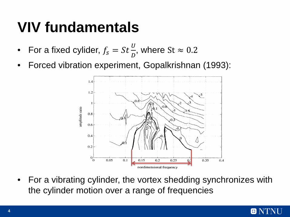
VIV fundamentals • For a fixed cylider, 𝑓𝑠 = 𝑆𝑆 𝑈

𝐷, where St ≈ 0.2

• Forced vibration experiment, Gopalkrishnan (1993):

• For a vibrating cylinder, the vortex shedding synchronizes with the cylinder motion over a range of frequencies

5

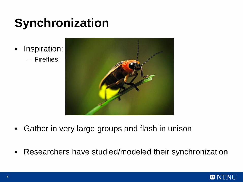
Synchronization

• Inspiration: – Fireflies!

• Gather in very large groups and flash in unison

• Researchers have studied/modeled their synchronization

6

Fireflies

• Hanson (1978) did experiments with periodically flashing light. How does the firefly synchronize? – ω0 : Firefly natural frequency – ωe : Frequency of flashing light

• Findings:

– For a range of ωe close to ω0 the firefly synchronizes – If ωe is too far from ω0, the firefly does not keep up.

• Note similarities with vortex shedding!

7

Firefly modeling 𝜙𝑒: Phase of flashing light. Flash when 𝜙𝑒 = 0 𝑑𝜙𝑒𝑑𝑑

= 𝜔𝑒: Frequency of flashing light

𝜙𝑓𝑓𝑓: Phase of firefly • Model proposed by Ermentrout and Rinzel (1984):

𝑑𝜙𝑓𝑓𝑓𝑑𝑆

= 𝜔0 + 𝐴 sin 𝜙𝑒 − 𝜙𝑓𝑓𝑓

𝜔0 𝐴

Slow down!

Speed up!

𝜙𝑒 − 𝜙𝑓𝑓𝑓

8

Back to VIV

• Assume the cross-flow excitation force can be expressed as 1

2𝜌𝐷𝑈2𝐶𝑣 cos𝜙𝑒𝑒𝑒

– 𝜙𝑒𝑒𝑒: Phase of the cross-flow excitation force – 𝜙�̇�: Phase of cylinder cross-flow velocity

• Synchronization model:

𝑑𝜙𝑒𝑒𝑒𝑑𝑆

= 𝐻(𝜙�̇� − 𝜙𝑒𝑒𝑒)

• How to find 𝐻?

Phase difference between velocity and force

(Similar to Ermentrout and Rinzel)

9

Finding 𝐻, the synchronization function • In the range of synchronization, assume

𝐶𝑒𝑒𝑒 𝜔 = 𝐶𝑒𝑒𝑒,𝑚𝑚𝑒 cos 𝜃 𝜔 • Plot 𝜔 versus 𝜃 based on VIVANA’s 𝐶𝑒𝑒𝑒:

Freq

uenc

y

Max freq = 1.5 fs

Freq = fs

fs = Strouhal frequency Phase difference

Min freq = 0.6 fs

10

Cross-flow hydrodynamic force model

1. Excitation with synchronization 2. Hydrodynamic damping 3. Added mass, 𝐶𝑚𝑓 = 1

11

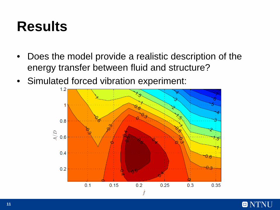
Results

• Does the model provide a realistic description of the energy transfer between fluid and structure?

• Simulated forced vibration experiment:

12

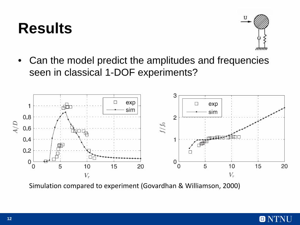
Results

• Can the model predict the amplitudes and frequencies seen in classical 1-DOF experiments?

Simulation compared to experiment (Govardhan & Williamson, 2000)

13

Results

Elastic cylinder in shear flow (NDP High Mode VIV tests) • Linear beam FE model • Hydrodynamic force calculated at every node • Time integration using Newmark-β

14

Results

Elastic cylinder in shear flow

15

Results

Elastic cylinder in shear flow Cross-flow response compared to experiment:

solid lines = simulated diamonds = measured

16

Results

• Flexible cylinder in oscillating flow • Experiments by Fu et al. (2014)

17

Results

• Flexible cylinder in oscillating flow • KC = 178, UR,max = 6.5:

18

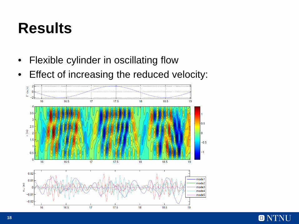
Results

• Flexible cylinder in oscillating flow • Effect of increasing the reduced velocity:

19

Concluding remarks

• So far: – A time domain model of the hydrodynamic forces relevant to VIV

has been established. – The model provides realistic results

• Future work: – How to combine the model with Morison’s eq. to include drag

forces? How does drag amplification occur? – Other PhD projects:

• Tor Huse Knudsen: Interaction between VIV and internal flow (deep ocean mining)

• Jan Vidar Ulveseter: Effect of nonlinear damping (soil or structural)

20

THANK YOU FOR YOUR ATTENTION!